
Submitted:
27 August 2025
Posted:
27 August 2025
You are already at the latest version
Abstract
Hyperspectral imaging (HSI) systems often suffer from complex noise degradation during the imaging process, significantly impacting downstream applications. Deep learning-based methods, though effective, rely on impractical paired training data, while traditional model-based methods require manually tuned hyperparameters and lack generalization. To address these issues, we propose SS³L (Self-supervised Spectral-Spatial Subspace Learning), a novel HSI denoising framework that requires neither paired data nor manual tuning. Specifically, we introduce a self-supervised spectral-spatial paradigm that learns noisy features from noisy data rather than paired training data, based on spatial geometric symmetry and spectral local consistency constraints. To avoid manual hyperparameter tuning, we propose an adaptive rank subspace representation and a loss function designed based on the collaborative integration of spectral and spatial losses via noise-aware spectral-spatial weighting, guided by the estimated noise intensity. These components jointly enable a dynamic trade-off between detail preservation and noise reduction under varying noise levels. The proposed SS$^3$L embeds noise-adaptive subspace representations into the dynamic spectral-spatial hybrid loss constrained network, enabling cross-sensor denoising through prior-informed self-supervision. Experimental results demonstrate that SS$^3$L effectively removes noise while preserving both structural fidelity and spectral accuracy under diverse noise conditions. The source code will be available at {https://github.com/yinhuwu/SS3L}
Keywords:
self-supervised learning
; hyperspectral image denoising
; hyperspectral imaging
; hyperparameterfree methods
1. Introduction
Hyperspectral images (HSIs) retain rich spectral and spatial information, and have been extensively explored in various kinds of applications, such as biology, ecology and geoscience [1,2,3]. However, HSIs are often contaminated by noise, which adversely impacts the performance of downstream tasks such as classification, detection, and quantitative analysis, thereby undermining the accuracy and reliability of HSI-based decision-making. Consequently, numerous HSI denoising techniques have been proposed to address this challenge [4,5].
HSI denoising methods can be broadly categorized into traditional model-based methods and deep-learning-based methods. Traditional approaches typically formulate HSI denoising as an ill-posed inverse problem, which is addressed by incorporating regularization terms based on prior knowledge to transform it into a well-posed problem. For instance, studies in [1,2,4,5,6] encoded both global low-rank and local smoothness priors using the total variation (TV) technique for HSI denoising. Concurrently, Zhuang et al. exploited the non-local low-rank prior by applying a low-rank constraint to non-local HSI blocks in [7]. To address sparse noise, some methods modeled these noise types as sparse components, characterized using distinct paradigms such as the norm in [8], the norm in [9] and Schatten-p norm in [10]. Although knowledge-driven methods effectively capture inherent HSI characteristics, they are highly sensitive to parameter settings, including the rank of the low-rank prior and the number of iterations.
Recent advances in deep learning have demonstrated superior performance in HSI denoising, particularly through convolutional neural networks (CNNs) and transformer-based methods [11,12,13]. For example, Chang et al. [11] introduced HSI-DeNet to evaluate the efficacy of CNNs for HSI denoising, while [12] developed a 3D attention network for this task. Similarly, Zhang et al. [13] proposed a three-dimensional spatial-spectral attention transformer for HSI denoising. Compared to traditional model-based methods, these supervised approaches learn a nonlinear mapping or function using paired clean-noisy data, enabling intuitive and rapid inference. However, their performance depends heavily on the availability and quality of training data, as paired clean-noisy HSI datasets remain scarce in practice. Additionally, hyperspectral sensors exhibit substantial variations in specifications, which means models trained on data from one sensor may not generalize well to HSI from other sensors.
These issues have spurred interest in data-independent approaches, such as self-supervised learning [14,15,16] and unsupervised learning [17,18,19]. A prominent example is Noise2Noise (N2N) [14], a self-supervised method that learns noise distributions by training on multiple noisy observations of the same scene. Another approach, Deep Image Prior (DIP) [17], employs a randomly initialized neural network to generate clean images by mapping a fixed random input (e.g., white noise) to a noise-free output. However, as an iterative optimization-based method, DIP’s performance is highly sensitive to handcrafted hyperparameters (e.g., learning rate, early stopping) and the choice of loss function. Furthermore, adapting the N2N framework to HSI denoising remains challenging. Unlike RGB images with three spectral channels, HSI contains hundreds of spectral bands, making direct application of RGB-oriented N2N methods suboptimal for HSI. These limitations hinder the generalizability of existing data-independent methods when processing remote sensing HSI across diverse scenes and sensors.
Despite the success of existing HSI denoising methods, two fundamental challenges remain: (1) supervised deep learning approaches require paired noisy-clean images, which are often unavailable in remote sensing, and (2) model-based methods are sensitive to hyperparameters and struggle with diverse noise types. To address these issues, we propose SS3L (Self-supervised Spectral-Spatial Subspace Learning), a novel dual-constrained framework that integrates self-supervised learning with subspace representation (SR). By leveraging intrinsic redundant features, we design a spectral-spatial hybrid loss function that integrates adaptive rank SR (ARSR), thereby constructing an end-to-end self-supervised framework robust to different noise conditions and various imaging systems. Specifically, we introduce a noise variance estimator called Spectral-Spatial Hybrid Estimation (SSHE) by exploring spatial-spectral local self-similarity priors, which quantifies the noise intensity by analyzing adjacent spectral differences and local variance statistics as the first step of the denoising process. Based on the spectral-spatial isotropy of noise and the structural consistency prior of natural scenes, we develop spatial checkerboard downsampling and spectral difference downsampling strategies to construct complementary spatial and spectral constraints. An adaptive weighting function conditioned on the noise variance estimated via SSHE is employed to formulate the Adaptive Weighted Spectral-Spatial Collaborative Loss Function (AWSSCLF), ensuring robustness under varying noise levels. Concurrently, the ARSR algorithm determines the optimal subspace dimension by dynamically adjusting the latent rank based on the estimated noise energy. Under the constraints of the proposed AWSSCLF, a lightweight network is employed to learn the denoising task within the subspace obtained via ARSR, thereby completing the construction of an end-to-end self-supervised denoising framework.
The main contributions of this article are as follows:
- 1.
- We propose SS3L, a spatial-spectral dual-domain self-supervised framework that embeds domain priors into both model design and optimization via ARSR. By enforcing cross-scale consistency through spatial and spectral downsampling, the framework achieves effective noise-signal disentanglement from a single noisy HSI without corresponding clean image supervision.
- 2.
- We design a spectral-spatial hybrid loss function named AWSSCLF with physics constraints: geometric symmetry and inter-band spectral correlation. Its noise-adaptive weighting mechanism derived from SSHE automatically prioritizes structural fidelity under low noise and enhances denoising under high noise, achieving adaptability to different imaging systems.
- 3.
- The proposed ARSR guided by singular value energy distribution and noise energy estimation can dynamically adjust the subspace rank to balance signal fidelity and noise separation, ensuring robustness at varying noise levels.
The rest of this article is organized as follows. Data-independent deep learning methods and SR techniques are reviewed in Section II. The proposed method is presented in Section III. Experimental results are shown in Section IV. Finally, conclusions are drawn in Section V.
2. Related Works
In this section, we analyze three categories of data-independent HSI denoising approaches: model-based and knowledge-driven approaches, self-supervised learning-based techniques, and unsupervised learning-based methods.
2.1. Model-Based Methods
Traditional knowledge-driven methods formulate the HSI denoising problem as an ill-posed inverse problem, subsequently regularizing it into a well-posed formulation via manually designed terms that enforce prior spectral-spatial constraints.
HSI denoising exploits three core data priors: (1) local/global low-rankness, (2) local smoothness, and (3) non-local self-similarity across spatial-spectral domains to construct the regularization terms. The low-rank prior originates from the intrinsic subspace structure of HSI data cubes, where nuclear norm minimization (e.g., weighted nuclear norm minimization (WNNM) [20], tensor robust principal component analysis (TRPCA) [21]) and low-rank matrix/tensor decomposition (e.g., low-rank matrix recovery (LRMR) [1], non-local low-rank tensor decomposition [22]) serve as dominant regularization strategies. Local smoothness priors enforce spatial consistency by constraining neighboring pixel variations, typically implemented through TV regularizers such as LRMR-TV [2], local low-rank spatial-spectral TV (LLRSSTV) [6], and 3D correlation TV (3DCTV) [23]. Non-local self-similarity priors (NLSSP) leverage redundant spatial patterns, integrated via hybrid frameworks like BM4D [24], Kronecker basis representation (KBR) [25], and Non-local Meets Global (NG-meets) [3]. Sparse representation techniques [5,26] and tensor factorization variants [4,7] further complement these approaches.
However, these optimization-based approaches are highly sensitive to parameter selection, including rank of tensor decomposition, patch size, group numbers, regularization weights, iterations and so on. Furthermore, handcrafted constraint terms struggle to adapt to complex noise profiles and diverse HSI data distributions. These limitations hinder the generalization of traditional methods when processing HSIs under various noise conditions.
2.2. Self-Supervised Denoising
Although supervised deep learning methods have demonstrated notable empirical success in HSI denoising, acquiring large-scale paired noisy-clean training data, especially remote sensing HSIs, remains challenging. To circumvent this limitation, self-supervised denoising frameworks have been developed to learn intrinsic image features directly from noisy observations. Pioneering work by Lehtinen et al. [14] laid the theoretical foundation for training denoising networks without clean images. Their study shows that, under the assumption of zero-mean and independent noise, a network trained to map between two independently corrupted observations of the same region can implicitly learn to recover the clean image. Formally, given two noisy observations:
where are independent noise vectors. Minimizing the expected loss:
is theoretically equivalent to supervised training with clean image :
This surprising result enables the N2N framework to train a denoiser using aligned noisy-noisy image pairs to estimate the clean image by minimizing the loss .
Based on N2N, Neighbor2Neighbor (Ne2Ne) [16] eliminated the need for aligned pairs by subsampling random neighbors from a single noisy image to generate training pairs. Zero-Shot Noise2Noise (ZSN2N) [27] proposed a symmetric downsampler based on the random neighbor downsampler in Ne2Ne for single-image denoising. Meanwhile, methods like Noise2Void (N2V) [28], Noise2Self (N2S) [29], and Signal2Signal (S2S) [30] employed blind-spot networks (BSNs) to predict target pixels using surrounding neighborhoods, circumventing N2N’s requirement for two independent noisy observations.
All of the above self-supervised networks are designed for RGB images and extending a single-band version of the network directly to the HSI case, band-by-band, often leads to suboptimal performance, which has been presented by the experiment in [26]. There are numerous self-supervised techniques designed for HSI denoising recently. In [31], Qian et al. extended the work of N2N by using two neighboring bands of an HSI as the noisy-noisy training pairs. Zhuang et al. [26] proposed Eigenimage2Eigenimage (E2E) by combining SR [32] with Ne2Ne [16]. E2E learned noise distribution using paired noisy eigenimages obtained by SR instead of HSI data with full bands to overcome the constraint of the number of frequency bands. However, E2E remains a self-supervised method and inherits N2N’s constraints: dependence on curated training data and limited robustness for diverse HSI datasets.
2.3. Unsupervised Methods
DIP [17], a classic unsupervised-learning denoising method, achieves single-image denoising by exploiting the inherent inductive bias of randomly initialized neural networks. Specifically, neural networks prioritize fitting the underlying image structure over noise artifacts when mapping random input to noisy observations. By optimizing the network to reconstruct the noisy input from random noise, guided by the following loss function:
the network captures the clean image’s latent features before overfitting to noise. Early stopping at an optimal iteration step thus yields a denoised output, circumventing the need for pre-trained models or paired training data.
Sidorov et al. [19] extended DIP to HSI denoising, while Miao et al. [33] proposed a disentangled spatial-spectral DIP framework based on HSI decomposition via a linear mixture model. Qiang et al. [34] introduced a self-supervised denoising method combining spectral low-rankness priors with deep spatial priors (SLRP-DSP), and Shi et al. [18] developed a double subspace deep prior approach by integrating sparse representation into the DIP framework.
Although these DIP-based methods achieve notable results and preserve HSI spatial-spectral details effectively, they inherit critical limitations. The DIP-based methods are inherently highly sensitive to iteration counts: insufficient iterations yield suboptimal denoising, while excessive iterations lead to overfitting to noise. Furthermore, integrating handcrafted prior constraints reintroduces the pitfalls of traditional methods: sensitivity to hyperparameters in regularization terms.
To address these issues, we propose a HSI denoising framework named SS3L that generalizes robustly under diverse scenarios, including varying noise levels, noise types, and HSI datasets from heterogeneous sensors. Unlike existing approaches that rely on network architectures designed to model noise structure, our framework learns noise distributions by focusing on the inherent characteristics of both noise and HSI data, thereby decoupling denoising performance from handcrafted priors or sensor-specific training data.
3. Proposed Method
3.1. Overview of SS3L Framework
In this section, we introduce the proposed SS3L (Self-supervised Spectral-Spatial Subspace Learning) framework for HSI denoising. As illustrated in Figure 1, SS3L consists of two key components:
- Adaptive Rank Subspace Representation (ARSR): A dynamic rank subspace decomposition is applied to the noisy HSI, guided by a hybrid spatial-spectral noise estimation strategy. This step captures the intrinsic low-dimensional structure of the image while suppressing noise.
- Adaptive Weighted Spectral-Spatial Collaborative Loss Function (AWSSCLF): Constructed based on spatial geometric symmetry and spectral continuity priors, AWSSCLF incorporates a sigmoid-based adaptive weighting mechanism that dynamically balances the two loss components according to the estimated noise level, ensuring robust and effective denoising under diverse conditions.
The SS3L framework adopts a dual-path training mechanism comprising spatial and spectral supervision branches. Both branches rely on subspace representations derived through ARSR, which dynamically selects the latent dimension based on noise intensity. The spatial path leverages checkerboard downsampling to create paired sub-images, which facilitates a regression-consistency loss design. In parallel, the spectral path performs spectral difference downsampling, with each sub-cube undergoing ARSR before being processing by the network.
The noise variance, estimated through Spectral-Spatial Hybrid Estimator (SSHE), generates adaptive coefficient that balance influence of the spatial and spectral losses. These components are then integrated into a unified loss function, termed the AWSSCLF, to guide the self-supervised learning of the network without requiring any clean ground truth.
In the following subsections, we first formulate the denoising problem and define the mathematical notation used throughout the method. Then we detail each component of the proposed method.
3.2. Problem Formulation
We begin by formulating the HSI denoising problem. In practice, HSIs are often degraded by a combination of additive Gaussian noise (i.e., sensor and atmosphere effects) and sparse noise (e.g. stripes, dead pixels, or impulse interference). These corruptions collectively deteriorate both spatial and spectral fidelity, challenging downstream processing tasks.
The observed noisy HSI is modeled as the sum of a clean image , additive Gaussian noise , and sparse noise :
where denote the degraded noisy HSI and clean HSI, respectively; represents the additive Gaussian noise and indicates the sparse noise.
The SR can represent the hyperspectral vectors based on the high spectral correlation [8]:
where denotes the eigenimages of the SR, in which is the dimension of the subspace and hyperparameter of the SR (i.e., rank r) fixed at in [26], indicates the mode-3 product of a tensor with a matrix is denoted as , resulting in a tensor of size . The matrix consists of the first r spectral eigenvectors extracted from an orthogonal matrix satisfying , in which and is the identity matrix.
The SR of the noisy HSI with rank r can be formulated as
where denotes the subspace decomposition of with rank r, yielding the coefficient tensor and the basis matrix .
3.3. Adaptive Rank Subspace Representation
The projection of noisy HSIs into a low-dimensional orthogonal subspace enables simultaneous data dimensionality reduction (enhancing computational efficiency) and structural fidelity preservation with noise attenuation. However, conventional fixed-rank SR methods are inherently limited by their static design. These methods impose a binary trade-off: higher ranks retain more high-frequency details (e.g., textures, edges) but tend to preserve more noise under heavy corruption, whereas lower ranks tend to over-smooth the data, which suppresses noise effectively but also leads to loss of semantically important structures. This fundamental rigidity prevents fixed-rank SR from adapting to varying noise levels across different scenarios.
To break the limitation of fixed-rank decomposition, we propose an adaptive framework called ARSR, which dynamically adjusts the subspace rank based on localized noise levels. This is achieved by integrating SSHE, a spectral-spatial hybrid estimation method that quantifies noise variance through joint analysis of spatial homogeneity and spectral correlation, with singular value thresholding to infer optimal SR rank. ARSR enables context-aware dimensionality reduction: in clean, detail-rich regions, it preserves higher ranks (e.g., 12–16), while in noise-dominated areas, it applies more aggressive truncation (e.g., 3–4), thus resolving the fixed-rank trade-off with adaptive precision.
We first introduce SSHE, followed by the ARSR mechanism.
Noise Estimation via SSHE
To accurately estimate noise levels, we design the SSHE method by combining two complementary strategies: Adjacent Band Estimation (ADE) and Marchenko-Pastur Variance Estimation (MPVE).
- ADE leverages the strong spectral correlation between neighboring HSI bands. Since signal components typically vary smoothly between adjacent bands, their differences tend to be small, while uncorrelated noise remains, or becomes more prominent in the residuals.
- MPVE exploits the statistical behavior of noise in the spatial domain. By unfolding the HSI into a matrix and analyzing its singular value distribution, which follows the Marchenko-Pastur (MP) law [35], the noise variance is estimated from the middle singular values.
The formulation of ADE is presented in Eq. (7).
in which denotes the differential matrix of band images and , represents the median of , (Median Absolute Deviation) quantifies the dispersion of . For data that follow a normal distribution, the standard deviation relates to MAD as ( see [36]). Therefore, multiplying by 1.4826 can convert MAD into the estimation of the standard deviation of the noise in noisy HSI data .
MPVE is designed by exploring the statistical regularity of the singular values of a random matrix. Specifically, we unfold the HSI tensor along the spectral mode into a matrix , where is the number of spatial pixels and is the number of spectral bands.
The matrix is centered and normalized by its Frobenius norm, followed by singular value decomposition (SVD) as:
where contains the singular values in descending order.
The empirical noise power is estimated from the bulk of the singular values by removing extreme outliers. Specifically, we compute:
which captures the energy level predominantly associated with noise. This estimate is then corrected using the expectation of the MP distribution [35], yielding the final noise variance estimation as:
where c is the matrix aspect ratio, and the MP expectation accounts for finite-sample bias in random matrices.
By combining ADE (spectral-domain analysis) and MPVE (spatial-domain analysis), SSHE provides robust and accurate estimation of the noise variance under various HSI conditions.
where the weight reflects the relative reliability of ADE and MPVE. The estimated noise variance can be used to guide the following steps.
Notably, the noise estimation process does not require exact numerical accuracy. Instead, it serves to provide a coarse but meaningful estimation of the noise trend, which is sufficient to guide the subsequent self-supervised denoising module. This design enhances the robustness of our framework and reduces the dependence on dataset-specific tuning.
3.4. MP-based Variance Estimation (MPVE)
MPVE is designed by exploring the statistical regularity of the singular values of a random matrix. Specifically, we unfold the HSI tensor along the spectral mode into a matrix , where represents the number of spatial pixels and is the number of spectral bands.
Under the assumption of additive white Gaussian noise (AWGN), each row of corresponds to an independent spectral sample contaminated by noise, allowing to be modeled as a random matrix with i.i.d. entries in its noise-dominated part. According to the Marchenko–Pastur (MP) law [35], the empirical spectral distribution of the sample covariance matrix converges to the MP distribution:
where is the aspect ratio and .
In practice, we normalize the matrix by its Frobenius norm:
where contains singular values in descending order.
The empirical noise power is estimated from the bulk of the spectrum by excluding extreme outliers:
This estimate is further corrected by the MP expectation to account for the aspect ratio:
By combining ADE (spectral-domain analysis) and MPVE (spatial-domain analysis), SSHE achieves a robust and accurate estimation of the noise variance under various HSI conditions.
Adaptive Rank Selection Guided by Noise Statistics
The optimal SR rank is adaptively determined by the estimated variance . This adaptive mechanism simultaneously accounts for the statistical characteristics of normal distributions and the energy-dominated physical meaning of singular values.
Specifically, we determine the number of components to retain based on the magnitude of singular values obtained from SVD relative to the estimated noise variance and matrix aspect ratio. The selection criterion is given by:
where , represent the i-th and -th singular values, is the estimated noise variance, n denotes the column dimension of the reshaped HSI matrix (the band numbers B), and is the matrix aspect ratio, with representing the total number of spatial pixels. The index i corresponding to the last singular value that satisfies this inequality is selected as the optimal SR rank. The threshold is grounded in the MP distribution [35], which describes the asymptotic singular value distribution of random Gaussian matrices. It establishes a theoretical upper bound on noise-induced singular values. Singular values exceeding this threshold are considered to carry meaningful signal information, whereas smaller ones are dominated by noise.
In the context of SVD, singular values quantify the energy of different components in the data. Therefore, distinguishing signal from noise becomes a matter of identifying where this energy drops below the noise-dominated boundary. The proposed criterion effectively leverages both the statistical behavior of random matrices and the physical significance of singular values, enabling a noise level aware adaptive rank selection mechanism. Notably, this approach is adaptive to matrix dimensionality and avoids reliance on empirically tuned thresholds, thereby preserving signal structures while suppressing noise-induced artifacts.
It is worth noting that SSHE is primarily designed for dense Gaussian-like noise, which typically dominates the total noise energy in hyperspectral imagery. The estimated noise variance serves as a coarse but meaningful reference for subsequent self-supervised denoising, rather than as an exact measure, and sparse noise components (e.g., stripes, impulse noise) are handled in later stages of our framework (e.g., AWSSCLF, ARSR). In practical remote sensing scenarios, such sparse noise usually affects only a small fraction of pixels or bands and exhibits much lower total energy, making the current variance-based approach a valid approximation for modeling the dominant noise components. Nevertheless, in extreme and rare cases where noise consists purely of sparse, non-Gaussian patterns, the Gaussian-based estimation in Eq. (7) may be less effective, and integrating robust statistical estimators or sparse modeling techniques could further enhance flexibility.
3.5. Adaptive Weighted Spatial-Spectral Collaborative Loss Function
To achieve robust denoising under diverse noise conditions, we further introduce an adaptive weighting mechanism. This mechanism dynamically balances the contributions of spatial and spectral constraints based on the estimated noise characteristics, ensuring optimal performance without requiring manual hyperparameter tuning. In the following sections, we detail the spatial downsampling strategy and spatial loss formulation, followed by the spectral downsampling and spectral loss, before finally discussing how their adaptive combination leads to an effective spatio-spectral denoising framework.
3.5.1. Spatial Loss Function
Building upon the N2N learning paradigm shown in Eq. (2), we adopt symmetric downsampling to generate multiple noisy observations from a single input sample for unsupervised noise distribution learning. Unlike conventional random neighborhood downsampling in Ne2Ne [16] and E2E [26], which introduces spatially uneven degradation, the checkerboard-patterned symmetric downsampling decomposes the original HSI into two geometrically balanced sub-images, preserving structural information while maintaining consistent i.i.d. noise among pixels.
The spatial downsampler, denoted as operates on eigenimages derived from ARSR. As illustrated in Figure 2: employs checkerboard-patterned decimation to generate two spatially complementary sub-images , . To improve the computational efficiency of spatial downsampling, we implement two 2D convolutional layers with customized kernels: and with stride 2 in order to implement the proposed spatial downsampling by convolutional operations.
It is worth emphasizing that the proposed checkerboard sampling differs fundamentally from the random neighborhood subsampling adopted in [14]. In [14], within each block, two adjacent pixels are randomly selected and assigned to and , resulting in a stochastic and spatially varying sampling pattern. By contrast, the proposed method employs a deterministic and symmetric checkerboard allocation, where pixels are consistently assigned to and across the entire image. This symmetry ensures uniform spatial frequency coverage and eliminates randomness, thereby improving the stability and reproducibility of self-supervised training.
Based on the spatial downsampler , the spatial loss function is defined as
where denotes the regression loss and denotes the consistency loss.
A residual learning strategy is employed, in which the network is trained to predict the noise component rather than the clean HSI itself. The clean HSI is subsequently recovered by subtracting the estimated noise from the noisy observation:
The regression and consistency terms are formulated as
where
represents the estimation of the clean downsampled HSI from its noisy counterpart . Here, denotes the downsampling operator with kernel .
The regression loss (16) enforces fidelity between the downsampled noisy observations and their denoised counterparts, thereby encouraging accurate residual prediction across multiple views. The consistency loss (17) serves as a regularization term by encouraging approximate commutativity between the network and the downsampling operator:
Such approximate commutativity is sufficient to stabilize training, preserve multi-scale spatial structures, and provide meaningful supervision signals in the self-supervised setting, ultimately improving the robustness and performance of hyperspectral image denoising.
3.5.2. Spectral Loss Function
Given the rich spectral information in HSIs and their inherent smoothness prior, we propose spectral downsampling to effectively exploit this prior and construct a spectral loss function based on the spectral downsampler. This approach not only enhances the spectral consistency but also complements the spatial loss function which is designed to enhance spatial consistency constraints.
While spatial downsampling operates on geometric structures, spectral downsampling targets inter-band correlations: split the HSI into two sub-cubes along the spectral axis, odd and even indexes, and a neighborhood-based smoothing is applied within each sub-cube by averaging adjacent spectral bands. As shown in Figure 3, this process decomposes a 6-band HSI into two 2-band sub-cubes, where the averaged bands inherit material-specific signatures.
Formally, the spectral downsampler takes an input HSI , producing two spectrally subsampled HSIs and . If B is odd, the last band is duplicated to ensure equal dimensionality. We applied two 1D Conv with kernels and to accelerate the down sampling process.
The spectral loss function is theoretically similar to the spatial loss function, but the implementation is quite different. While the spatial loss directly applies spatial downsampling operators to eigenimages and feeds the reduced-resolution outputs into the network , this approach is fundamentally incompatible with spectral-domain processing. Even when employing 3D convolutional layers to address channel dimensionality constraints, it remains infeasible to reconstruct the denoised results with processed sub-eigenimages with the eigenmatrix due to structural mismatches introduced spectral downsampling.
To resolve this, as illustrated in the lower part of Figure 1 (a), our method employs ARSR on spectrally downsampled HSIs . This decomposition produces representative eigenimages which are then processed by the network to yield denoised subsampled data . By embedding spectral downsampling into the spatial loss function, we formalize the spectral loss paradigm in Eq. (20):
where, denote the spectrally sub-samples; represent the denoising results corresponding to .
3.5.3. Collaboration of Spatial and Spectral Losses
A fixed-weight combination of spatial and spectral losses fails to capture the scenario-specific priority each constraint requires in real-world denoising tasks. For instance, spatial priors dominate in high-noise regimes to recover structural coherence, while spectral priors excel at low-noise levels by preserving material-specific signatures. To enable robustness to different scenarios, we formulate the spectral-spatial collaborative loss function as:
where, controls the balance between the two loss terms, indicates the spatial loss in Eq. (14) and refers the spectral loss in Eq. (20).
To simultaneously leverage the advantages of both the spatial loss function in high noise scenario and spectral constraint under low noise condition, we propose a noise adaptive weighting function Eq. (24) with the estimated noise level from Eq. (10):
where dynamically adjusts the influence of spectral and spatial losses based on the estimated noise level ; k is a parameter that can adjust the curvature of the function curve; denotes the threshold that is generated by ensuring that the signal-to-noise ratio is closest to 10 dB. To distinguish between high and low noise levels, we use SNR = 10 dB as a threshold. This level of noise significantly affects high-frequency information (e.g., texture, edge details), making noise suppression and detail preservation a challenging trade-off. The proposed AWSSCLF not only enhances robustness against diverse noise levels but also eliminates the need for manually tuned hyperparameters, ensuring robust performance.
3.6. End to End Self-Supervised Denoising
With the subspace projection and hybrid loss functions in place, we now describe the end-to-end self-supervised learning procedure. The full workflow of the proposed SL framework is summarized in Algorithm 1 and shown in Figure 1.
The Network used in this work is a lightweight network consisting of three 2D convolutional layers and two LeakyReLU layers. During training, we first apply ARSR to reduce the dimensionality of noisy HSI while preserving its intrinsic structure. The resulting eigenimages serve as the basis for designing spatial and spectral loss functions aimed at enhancing consistency. The spatial loss follows a downsampling-based strategy to enforce spatial consistency, while the spectral loss ensures fidelity along the spectral dimension. These loss functions are computed independently but combined through a noise-aware adaptive weighting scheme. The integrated loss function, AWSSCLF, is used to constrain a lightweight network within a self-supervised learning framework, as shown in Figure 1 (a). The network is trained via gradient descent to optimize . Once trained, it is applied to the original noisy observation to estimate the denoised image, as illustrated in Figure 1 (b): .
4. Experiments
4.1. Experimental Setup
4.1.1. Datasets and Evaluation Metrics
We evaluate the proposed method on six HSI datasets under two experimental settings: simulated noise removal and real noise removal. All datasets are preprocessed by removing low-SNR bands, such as those affected by water vapor absorption, to ensure consistent and fair evaluation. For large-scale datasets, spatial patches of size are extracted for training and evaluation.
For simulated noise removal, experiments are conducted on the Washington DC Mall (WDCM) dataset, the Kennedy Space Center (KSC) dataset, the GF-5 dataset [37], and the AVIRIS dataset [37]. Specifically, WDCM consists of a single HSI of size , acquired by the AVIRIS sensor, with 191 bands retained after low-SNR band removal. KSC consists of a single HSI of size , also acquired by AVIRIS. The GF-5 dataset provides hyperspectral data of size , acquired by the AHSI sensor, with the number of bands reduced to 305 after removing low-SNR bands affected by atmospheric absorption. The AVIRIS dataset contains hyperspectral data of size , also collected using the AVIRIS sensor.
For real noise removal, experiments are conducted on the GF-5 and AVIRIS datasets (the same as in the simulated setting), as well as on the Indian Pines and Botswana datasets. The Indian Pines dataset consists of hyperspectral data of size , acquired by AVIRIS, while the Botswana dataset contains a HSI of size , acquired by the EO-1 Hyperion sensor.
To quantitatively assess the denoising performance, we adopt three commonly used evaluation metrics: mean of Peak Signal-to-Noise Ratio (mPSNR), mean of Structural Similarity Index (mSSIM), and mean of Spectral Angle Mapper (mSAM).
4.1.2. Implementation Details
Throughout all experiments across different HSI datasets and noise conditions, we set in Eq. (10) to 0.7 and k in Eq. (24) to 0.8.
Experiments of all methods were implemented in Python with PyTorch=1.13.1 on Ubuntu 22.04.5, using an Nvidia GeForce RTX 3090 GPU with 24GB memory. Model training was conducted on the same GPU, with 3000 training iterations. The Adam optimizer was used with parameters (0.9, 0.999) and a learning rate of 0.001.
It should be noted that certain traditional HSI denoising methods, such as NG-Meet, LRTF-DFR, LRMR, and FastHy, often require dataset-specific hyperparameter tuning to achieve optimal performance. In our experiments, we adopted the default hyperparameters provided by the original authors across all datasets without any manual adjustment. While this may lead to suboptimal performance for some methods in specific scenes, our proposed SS3L framework does not require any hyperparameter tuning, which demonstrates its robustness and stability across diverse datasets. The source code includes implementations of these methods. This design ensures a fair and reproducible comparison.
4.1.3. Comparison Methods
To evaluate the performance of the proposed method, we compared it with eight state-of-the-art methods. These include traditional approaches such as low-rank matrix recovery (LRMR) [1], non-local and global prior-based methods (NG-meet) [3], and tensor decomposition-based methods like LRTF-DFR [4] and L1HyMixDe [8]. Additionally, we considered a hybrid approach that combines traditional methods and Plug-and-Play deep regularization term (FastHy) [5]. The deep learning methods include the supervised methods: HSID-CNN [38] and QRNN3D [39], as well as the self-supervised method: Ne2Ne [16].
For HSID-CNN and QRNN3D, since our method operates in a self-supervised paradigm, we directly applied the pre-trained models provided by the original authors, instead of retraining them on our dataset, for a fair comparison. This approach was necessary since our experimental setup only involves six HSI datasets which are insufficient to meet the data requirements for training these supervised networks.
Methods HSID-CNN and QRNN3D take 32-band and 31-band HSIs as input, respectively. The HSI datasets used in this work are divided into patches with size with a step size of to be fed into these two networks. The results of these two methods are reconstructed via the resulting patches. The Ne2Ne was designed for RGB images. A single-band version was retrained on these HSI dataset and applied to the corresponding HSI datasets.
4.2. Simulated Noise Removal
To assess denoising performance, simulated noisy HSIs were generated by introducing zero-mean additive Gaussian noise to the data which had been normalized to the range [0, 1]. Each spectral band was independently corrupted with Gaussian noise , simulating band-specific sensor noise.
To comprehensively evaluate robustness for varying noise intensities, we constructed a fine-grained simulated noisy HSIs dataset consisting of 20 noise levels, with standard deviations with the scaled standard deviation ranging from 5 to 100). This approach provides a thorough assessment of the performance under diverse noise conditions and imaging scenarios.
We define five representative test scenarios (Cases 1-5), which capture key points for the noise intensity and cover both Gaussian and sparse noise situations. These serve as benchmarks for subsequent qualitative and quantitative analyses.
- Cases 1-4 : Gaussian noise with scaled noise levels of 5, 25, 50, and 100 was added to simulate various corruption intensities.
- Case 5: To evaluate robustness against sparse structural noise, stripe artifacts were introduced by injecting 200 randomly located 1-pixel-wide vertical stripes into 25% of randomly selected bands, superimposed on the data already corrupted with Gaussian noise at level 50.
4.2.1. Quantitative Comparison
The experimental results for mPSNR, mSSIM, and mSAM across 20 noise levels applied to the WDCM, KSC, GF-5, and AVIRIS datasets are presented in Figure 4. The proposed method achieves superior performance with varying noise levels on the WDCM, GF-5, and KSC datasets.
Traditional methods relying on simple priors (e.g., LRMR) underperform for diverse noise conditions. Composite prior-guided approaches such as L1HyMixDe and LRTF-DFR show limited effectiveness: L1HyMixDe achieves competitive results on WDCM and KSC under low noise, while LRTF-DFR performs moderately on WDCM with medium noise. Both degrade significantly in other scenarios.
NG-Meet, which integrates non-local and local priors, underperforms in low-noise regimes but excels under high noise. Notably, its PSNR increases with noise intensity, contrasting with the decline observed in other methods. FastHy, using deep networks as explicit regularizers via a plug-and-play framework, matches our method’s performance on WDCM and KSC but lags on GF-5 (1–3 dB gaps at noise levels 5–60). Supervised deep learning methods (QRNN3D, HSID-CNN) exhibit severe degradation without test-data fine-tuning, revealing training-data dependency. The self-supervised Ne2Ne method, though designed for RGB images, surpasses LRMR on multiple datasets. The AVIRIS dataset’s inherent noise in bands [107–116] and [152–171] leads to marginally lower metrics for our method compared to simulate noisy references. LRTF-DFR shows instability under non-uniform noise, with unstable performance fluctuations at different intensities.
Spectral recovery performance is further validated in Figure 5 and Figure 6, which compare reconstructed spectral curves in Case 2 and Case 5. Most comparison methods exhibit spectral shifting or distortion (Figure 5), while only our approach achieves optimal alignment with real curves (Figure 6). The proposed method gets the best match to real spectral trends and performs well in maintaining spectral fidelity.
Table 1 and Table 2 demonstrate the efficacy of our proposed SS3L , which learns intrinsic data structures directly from feature images rather than relying on manually designed regularization for denoising. While our method underperforms the advanced plug-and-play framework FastHy on the AVIRIS dataset in Cases 1 and 2, it achieves superior mPSNR values compared to most low-rank prior, local smoothness prior, and supervised learning-based approaches. Case 5, which combines Gaussian noise (level 50) and stripe artifacts, non-local self-similarity methods fail to balance noise removal with structural preservation. Low-rank-prior methods (L1HyMixDe, LRTF-DFR) excel only under low-noise conditions.
4.2.2. Qualitative Comparison
Visual results for Band 100 in Cases 2 and 4 on the WDCM and KSC datasets are shown in Figure 7 and Figure 8, respectively. The L1HyMixDe method performs well in Case 2 but deteriorates significantly under high-noise conditions (Case 4).
To simulate real-world conditions, we evaluated denoising performance on Gaussian-stripe mixed noise (Case 5). Noise was injected into 25% of randomly selected bands, resulting in visualized bands 111 (WDCM), 107 (KSC), 102 (GF-5), and 110 (AVIRIS). Notably, band 110 in AVIRIS belongs to the bands with real stripe noise (107–116), reflecting inherent low-SNR artifacts caused by atmospheric absorption.
As shown in Figure 9, most methods that are competitive under Gaussian noise fail to address mixed noise effectively: NG-Meet removes high-frequency noise but erases critical image details; LRTF-DFR fails to converge on KSC and GF-5 datasets; LRMR eliminates inherent AVIRIS tilted stripes but introduces artificial vertical stripes into denoised results; FastHy achieves competitive results on WDCM, KSC, and GF-5 but residual stripes remain when processing the AVIRIS dataset
It should be noted that these traditional methods, including NG-Meet, LRTF-DFR, LRMR, and FastHy, rely on manually tuned hyperparameters for optimal performance. In our experiments, we used the default parameters provided by the authors for all datasets, without dataset-specific adjustment. As a result, some methods may exhibit suboptimal performance in certain scenes. NG-Meet removes high-frequency noise but erases critical image details; LRTF-DFR fails to converge on KSC and GF-5 datasets; LRMR eliminates inherent AVIRIS tilted stripes but introduces artificial vertical stripes into denoised results; FastHy achieves competitive results on WDCM, KSC, and GF-5 but residual stripes remain when processing the AVIRIS dataset. In contrast, our SS3L framework, which requires no hyperparameter tuning, consistently delivers stable and reliable denoising results across all datasets, highlighting its practical advantage and robustness.
4.3. Real HSI Denoising Experiments
To further verify the adaptability of our proposed method on real noise scenes, we executed denoising experiments on four real-world HSI datasets Indian-pines, Botswana, AVIRIS and GF-5.
Each dataset represents distinct noise scenarios: Indian Pines: Gaussian noise with impulse artifacts (first band); Botswana: Low intensity Gaussian noise (final bands); AVIRIS: Medium intensity Gaussian noise (final bands); GF-5: Mixed Gaussian-stripe noise (final bands). Given the lack of ground truth, we take the band at a distance of 5 from the degraded band as the reference noise free sample.
As shown in Figure 10, all methods achieved satisfactory performance on low-to-medium noise (Botswana, AVIRIS), except supervised deep learning approaches, which perform ineffectively due to training data dependency. NG-Meet’s non-local priors suppressed noise but eroded fine details. L1HyMixDe removed noise completely but introduced luminance distortion. Methods relying on low-rank priors (LRMR, LRTF-DFR) struggled with sparse noise (e.g., stripes, salt-and-pepper), while NG-Meet eliminated such artifacts at the cost of over-smoothing. Ne2Ne excelled spatially but compromised spectral fidelity, as shown in prior simulations. Our method outperforms all comparison methods, effectively removing complex noise (atmospheric interference, stripes, dead pixels) while preserving structural and spectral integrity for all datasets.
The simulated and real noise removal experiments validate the superiority of our proposed method, which outperforms existing methods in both quantitative metrics and visual quality. By integrating ARSR into AWSSCLF, our method automatically removes complex noise from a single HSI input while maintaining robustness under varying noise strengths and across different imaging sensors (AVIRIS, Hyperion, AHSI), without requiring hyperparameter tuning.
4.4. Ablation Study
To analyze how each component in the proposed framework contributes to the denoising performance, we conducted an ablation study on WDCM dataset with different noise levels.
4.4.1. Effectiveness of ARSR and AWSSCLF
To verify the effectiveness of the proposed ARSR and AWSSCLF strategy, we conducted an ablation study with the following four cases as shown in Table 3 For reference, we also report the mPSNR computed between the noisy HSI and the ground truth, to better assess the effectiveness of the compared strategies. As shown in Figure 11 (a), the method without SR exhibits the poorest performance, leading to significant information loss in low-noise conditions. The method with a fixed low-rank () SR performs poorly under noise level below 20 (), whereas the fixed high-rank () SR variant performs poorly in medium- and high-noise conditions: noise level higher than 40 (). In contrast, our proposed ARSR, which dynamically adjusts the rank for SR based on estimated noise variance, consistently outperforms all fixed-rank variants under different noise levels.
The experimental results in Figure 11 (b) show that under different noise intensities, the spatial loss function and the spectral loss function are complementary. In low-noise scenarios (, noise level lower than 25), relying on spatial loss function results in a 3-5 dB mPSNR reduction, while spectral loss maintains optimal reconstruction quality. This trend significantly reverses when noise level increases (, noise level greater than 40): the performance decay rate of spectral loss function is larger than that of spatial loss, with the latter demonstrating superior noise robustness. The fixed-weight (=0.5) spatial-spectral hybrid loss, although theoretically balanced, exhibits a maximum deviation of 3.8 dB under varying noise levels. In contrast, our AWSSCLF, achieves consistently optimal performance under all noise levels ().
4.4.2. Effectiveness of Network Structure
To evaluate the impact of the network architecture within the proposed framework, we conducted ablation experiments on the WDCM dataset by replacing the network while keeping the other components unchanged. Specifically, the compared network structures include:
The experimental results shown in Figure 12 reveal that under low noise conditions: noise level in [5,10] (), the 3D Conv network achieves approximately 2 dB PSNR advantage through spectral feature aggregation, and the performance differences of the other methods is less than 0.8 dB. As noise intensity increases: noise level greater than 20 (), the differences of method performance becomes significant: HSIDeNet deteriorates to 20 dB at noise level 100 (); U-Net and the 3D model maintain 25 dB via spatial-spectral feature fusion; our 2D network sustains optimal performance under noise level in [20,100] ().
4.5. Performance Evaluation of the Proposed Noise Estimator
We evaluate the performance of the three proposed noise estimator: ADE, MPVE and SSHE.
Figure 13 shows the noise estimation results of LAE, ADE, and SSHE under noise levels in [5, 100]. By dynamically balancing spatial and spectral information (with ), SSHE achieves the closest approximation to the real noise variance, significantly outperforming both ADE and MPVE.
5. Conclusions
In this work, we proposed SS3L , which addresses two fundamental challenges in HSI denoising: (1) the paired-data dependency of supervised deep learning, and (2) the hyperparameter sensitivity of conventional model-based methods, by employing three key techniques. First, we introduce geometric symmetry and spectral local consistency priors via spatial checkerboard downsampling and spectral difference downsampling, enabling noise–signal disentanglement from a single noisy HSI without clean reference data. Second, we develop the Spectral–Spatial Hybrid Estimation (SSHE) to quantify noise intensity, guiding the Adaptive Weighted Spectral–Spatial Collaborative Loss Function (AWSSCLF) that dynamically balances structural fidelity and denoising strength under varying noise levels. Third, the Adaptive Rank Subspace Representation (ARSR), driven by singular value energy distribution and noise energy estimation, determines the optimal subspace rank without heuristic selection, embedding adaptive subspace representations into the self-supervised network. These components jointly construct a dual-domain, physics-informed self-supervised framework that learns cross-sensor invariant features without requiring paired data or manual hyperparameter tuning, thus achieving robustness across diverse imaging systems. Extensive experiments validate SS3L’s superiority in removing mixed noise types (e.g., Gaussian, stripe, impulse) and generalizing to unseen scenes, achieving competitive performance both in quantitative metrics and visual quality. The current limitations stem from fixed spectral regularization weights and single-scene optimization paradigm. Future work will explore integrating Deep Image Prior (DIP) inductive bias and non-local priors into this self-supervised framework to further enhance generalization across diverse scenarios.
Author Contributions
Conceptualization, Dongyang Liu; Data curation, Yinhu Wu; Funding acquisition, Zhang Junping; Methodology, Yinhu Wu and Zhang Junping; Project administration, Zhang Junping; Validation, Yinhu Wu; Writing—original draft, Yinhu Wu; Writing—review & editing, Yinhu Wu and Zhang Junping.
Funding
This research was funded by the National Natural Science Foundation of China, grant number 62271171.
Data Availability Statement
The hyperspectral datasets used in this study, including the Washington DC Mall (WDCM) and Kennedy Space Center (KSC) datasets, are publicly available from the AVIRIS data repository (https://aviris.jpl.nasa.gov/). The GF-5 and AVIRIS datasets used in this study were obtained from the work of [37], and are available from the corresponding author upon reasonable request.
Conflicts of Interest
The authors declare no conflict of interest.
Abbreviations
The following abbreviations are used in this manuscript:
| HSI | Hyperspectral Image |
| RS | Remote Sensing |
| SNR | Signal-to-Noise Ratio |
| PSNR | Peak Signal-to-Noise Ratio |
| SSIM | Structural Similarity Index Measure |
| MPSNR | Mean Peak Signal-to-Noise Ratio |
| MSSIM | Mean Structural Similarity Index Measure |
| ARSR | Adaptive Reduced Subspace Representation |
| AWSSCLF | Adaptive Weight Spatial-Spectral Collaborative Loss Function |
| N2N | Noise2Noise |
| DIP | Deep Image Prior |
| PCA | Principal Component Analysis |
| SVD | Singular Value Decomposition |
| CNN | Convolutional Neural Network |
References
- Zhang, H.; He, W.; Zhang, L.; Shen, H.; Yuan, Q. Hyperspectral Image Restoration Using Low-Rank Matrix Recovery. IEEE Transactions on Geoscience and Remote Sensing 2014, 52, 4729–4743. [CrossRef]
- He, W.; Zhang, H.; Zhang, L.; Shen, H. Total-Variation-Regularized Low-Rank Matrix Factorization for Hyperspectral Image Restoration. IEEE Transactions on Geoscience and Remote Sensing 2016, 54, 178–188. [CrossRef]
- He, W.; Yao, Q.; Li, C.; Yokoya, N.; Zhao, Q.; Zhang, H.; Zhang, L. Non-Local Meets Global: An Iterative Paradigm for Hyperspectral Image Restoration. IEEE Trans. Pattern Anal. Mach. Intell. 2022, 44, 2089–2107. [CrossRef]
- Zheng, Y.B.; Huang, T.Z.; Zhao, X.L.; Chen, Y.; He, W. Double-Factor-Regularized Low-Rank Tensor Factorization for Mixed Noise Removal in Hyperspectral Image. IEEE Transactions on Geoscience and Remote Sensing 2020, 58, 8450–8464. [CrossRef]
- Zhuang, L.; Ng, M.K. FastHyMix: Fast and Parameter-Free Hyperspectral Image Mixed Noise Removal. IEEE Transactions on Neural Networks and Learning Systems 2023, 34, 4702–4716. [CrossRef]
- He, W.; Zhang, H.; Shen, H.; Zhang, L. Hyperspectral Image Denoising Using Local Low-Rank Matrix Recovery and Global Spatial–Spectral Total Variation. IEEE Journal of Selected Topics in Applied Earth Observations and Remote Sensing 2018, 11, 713–729. [CrossRef]
- Zhuang, L.; Fu, X.; Ng, M.K.; Bioucas-Dias, J.M. Hyperspectral Image Denoising Based on Global and Nonlocal Low-Rank Factorizations. IEEE Transactions on Geoscience and Remote Sensing 2021, 59, 10438–10454. [CrossRef]
- Zhuang, L.; Ng, M.K. Hyperspectral Mixed Noise Removal By ℓ1-Norm-Based Subspace Representation. IEEE Journal of Selected Topics in Applied Earth Observations and Remote Sensing 2020, 13, 1143–1157. [CrossRef]
- Chen, Y.; Huang, T.Z.; Zhao, X.L. Destriping of Multispectral Remote Sensing Image Using Low-Rank Tensor Decomposition. IEEE Journal of Selected Topics in Applied Earth Observations and Remote Sensing 2018, 11, 4950–4967. [CrossRef]
- Zhang, H.; Qian, J.; Zhang, B.; Yang, J.; Gong, C.; Wei, Y. Low-Rank Matrix Recovery via Modified Schatten- p Norm Minimization With Convergence Guarantees. IEEE Transactions on Image Processing 2020, 29, 3132–3142. [CrossRef]
- Chang, Y.; Yan, L.; Fang, H.; Zhong, S.; Liao, W. HSI-DeNet: Hyperspectral Image Restoration via Convolutional Neural Network. IEEE Transactions on Geoscience and Remote Sensing 2019, 57, 667–682. [CrossRef]
- Shi, Q.; Tang, X.; Yang, T.; Liu, R.; Zhang, L. Hyperspectral Image Denoising Using a 3-D Attention Denoising Network. IEEE Transactions on Geoscience and Remote Sensing 2021, 59, 10348–10363. [CrossRef]
- Zhang, Q.; Dong, Y.; Zheng, Y.; Yu, H.; Song, M.; Zhang, L.; Yuan, Q. Three-Dimension Spatial–Spectral Attention Transformer for Hyperspectral Image Denoising. IEEE Transactions on Geoscience and Remote Sensing 2024, 62, 1–13. [CrossRef]
- Lehtinen, J.; Munkberg, J.; Hasselgren, J.; Laine, S.; Karras, T.; Aittala, M.; Aila, T. Noise2Noise: Learning Image Restoration without Clean Data. In Proceedings of the Proceedings of the 35th International Conference on Machine Learning; Dy, J.; Krause, A., Eds. PMLR, 10–15 Jul 2018, Vol. 80, Proceedings of Machine Learning Research, pp. 2965–2974.
- Zhu, H.; Ye, M.; Qiu, Y.; Qian, Y. Self-Supervised Learning Hyperspectral Image Denoiser with Separated Spectral-Spatial Feature Extraction. In Proceedings of the IGARSS 2022 - 2022 IEEE International Geoscience and Remote Sensing Symposium, 2022, pp. 1748–1751. [CrossRef]
- Huang, T.; Li, S.; Jia, X.; Lu, H.; Liu, J. Neighbor2Neighbor: Self-Supervised Denoising from Single Noisy Images. In Proceedings of the 2021 IEEE/CVF Conference on Computer Vision and Pattern Recognition (CVPR), 2021, pp. 14776–14785. [CrossRef]
- Lempitsky, V.; Vedaldi, A.; Ulyanov, D. Deep Image Prior. In Proceedings of the 2018 IEEE/CVF Conference on Computer Vision and Pattern Recognition, 2018, pp. 9446–9454. [CrossRef]
- Shi, K.; Peng, J.; Gao, J.; Luo, Y.; Xu, S. Hyperspectral Image Denoising via Double Subspace Deep Prior. IEEE Transactions on Geoscience and Remote Sensing 2024, 62, 1–15. [CrossRef]
- Sidorov, O.; Hardeberg, J.Y. Deep Hyperspectral Prior: Single-Image Denoising, Inpainting, Super-Resolution. In Proceedings of the 2019 IEEE/CVF International Conference on Computer Vision Workshop (ICCVW), 2019, pp. 3844–3851. [CrossRef]
- Gu, S.; Zhang, L.; Zuo, W.; Feng, X. Weighted Nuclear Norm Minimization with Application to Image Denoising. In Proceedings of the 2014 IEEE Conference on Computer Vision and Pattern Recognition, 2014, pp. 2862–2869. [CrossRef]
- Lu, C.; Feng, J.; Chen, Y.; Liu, W.; Lin, Z.; Yan, S. Tensor Robust Principal Component Analysis with a New Tensor Nuclear Norm. IEEE Transactions on Pattern Analysis and Machine Intelligence 2020, 42, 925–938. [CrossRef]
- Xue, J.; Zhao, Y.; Liao, W.; Chan, J.C.W. Nonlocal Low-Rank Regularized Tensor Decomposition for Hyperspectral Image Denoising. IEEE Transactions on Geoscience and Remote Sensing 2019, 57, 5174–5189. [CrossRef]
- Peng, J.; Wang, Y.; Zhang, H.; Wang, J.; Meng, D. Exact Decomposition of Joint Low Rankness and Local Smoothness Plus Sparse Matrices. IEEE Transactions on Pattern Analysis and Machine Intelligence 2023, 45, 5766–5781. [CrossRef]
- Maggioni, M.; Katkovnik, V.; Egiazarian, K.; Foi, A. Nonlocal Transform-Domain Filter for Volumetric Data Denoising and Reconstruction. IEEE Transactions on Image Processing 2013, 22, 119–133. [CrossRef]
- Xie, Q.; Zhao, Q.; Meng, D.; Xu, Z. Kronecker-Basis-Representation Based Tensor Sparsity and Its Applications to Tensor Recovery. IEEE Transactions on Pattern Analysis and Machine Intelligence 2018, 40, 1888–1902. [CrossRef]
- Zhuang, L.; Ng, M.K.; Gao, L.; Michalski, J.; Wang, Z. Eigenimage2Eigenimage (E2E): A Self-Supervised Deep Learning Network for Hyperspectral Image Denoising. IEEE Transactions on Neural Networks and Learning Systems 2024, 35, 16262–16276. [CrossRef]
- Mansour, Y.; Heckel, R. Zero-Shot Noise2Noise: Efficient Image Denoising without any Data. In Proceedings of the 2023 IEEE/CVF Conference on Computer Vision and Pattern Recognition (CVPR), 2023, pp. 14018–14027. [CrossRef]
- Krull, A.; Buchholz, T.O.; Jug, F. Noise2Void - Learning Denoising From Single Noisy Images. In Proceedings of the 2019 IEEE/CVF Conference on Computer Vision and Pattern Recognition (CVPR), 2019, pp. 2124–2132. [CrossRef]
- Batson, J.; Royer, L. Noise2Self: Blind Denoising by Self-Supervision. In Proceedings of the Proceedings of the 36th International Conference on Machine Learning (ICML), Long Beach, California, USA, June 2019; Vol. 97, Proceedings of Machine Learning Research (PMLR), pp. 524–533.
- Quan, Y.; Chen, M.; Pang, T.; Ji, H. Self2Self With Dropout: Learning Self-Supervised Denoising From Single Image. In Proceedings of the 2020 IEEE/CVF Conference on Computer Vision and Pattern Recognition (CVPR), 2020, pp. 1887–1895. [CrossRef]
- Qian, Y.; Zhu, H.; Chen, L.; Zhou, J. Hyperspectral Image Restoration With Self-Supervised Learning: A Two-Stage Training Approach. IEEE Transactions on Geoscience and Remote Sensing 2022, 60, 1–17. [CrossRef]
- Zhuang, L.; Bioucas-Dias, J.M. Fast Hyperspectral Image Denoising and Inpainting Based on Low-Rank and Sparse Representations. IEEE Journal of Selected Topics in Applied Earth Observations and Remote Sensing 2018, 11, 730–742. [CrossRef]
- Miao, Y.C.; Zhao, X.L.; Fu, X.; Wang, J.L.; Zheng, Y.B. Hyperspectral Denoising Using Unsupervised Disentangled Spatiospectral Deep Priors. IEEE Transactions on Geoscience and Remote Sensing 2022, 60, 1–16. [CrossRef]
- Zhang, Q.; Yuan, Q.; Song, M.; Yu, H.; Zhang, L. Cooperated Spectral Low-Rankness Prior and Deep Spatial Prior for HSI Unsupervised Denoising. IEEE Transactions on Image Processing 2022, 31, 6356–6368. [CrossRef]
- Marchenko, V.A.; Pastur, L.A. Distribution of eigenvalues for some sets of random matrices. Mathematics of the USSR-Sbornik 1967, 1, 457–483.
- Rousseeuw, P.J.; Croux, C. Alternatives to the Median Absolute Deviation. Journal of the American Statistical Association 1993, 88, 1273–1283.
- Kang, X.; Fei, Z.; Duan, P.; Li, S. Fog Model-Based Hyperspectral Image Defogging. IEEE Transactions on Geoscience and Remote Sensing 2022, 60, 1–12. [CrossRef]
- Yuan, Q.; Zhang, Q.; Li, J.; Shen, H.; Zhang, L. Hyperspectral Image Denoising Employing a Spatial–Spectral Deep Residual Convolutional Neural Network. IEEE Transactions on Geoscience and Remote Sensing 2019, 57, 1205–1218. [CrossRef]
- Fu, Y.; Liang, Z.; You, S. Bidirectional 3D Quasi-Recurrent Neural Network for Hyperspectral Image Super-Resolution. IEEE Journal of Selected Topics in Applied Earth Observations and Remote Sensing 2021, 14, 2674–2688. [CrossRef]
Figure 1.
Flowchart of the proposed SL framework. (a) Training process with dual-path supervision. The spatial and spectral loss branches are represented by orange and teal arrows, respectively. Each path incorporates Adaptive Rank Subspace Representation (ARSR) and contributes to the Adaptive Weighted Spatial-Spectral Collaborative Loss Function (AWSSCLF). (b) Inference stage using the trained denoising network .
Figure 2.
The spatial downsampler decomposes an HSI into two HSIs of half the spatial resolution by averaging diagonal pixels of non-overlapping patches band by band. In the above example the input is a image, and the output is two images.
Figure 2.
The spatial downsampler decomposes an HSI into two HSIs of half the spatial resolution by averaging diagonal pixels of non-overlapping patches band by band. In the above example the input is a image, and the output is two images.
Figure 3.
The spectral downsampler decomposes an HSI into two HSIs with half the spectral bands by separating odd and even bands. In the above example the input is a HSI with 6 bands, and the output is two HSIs with 2 bands.
Figure 3.
The spectral downsampler decomposes an HSI into two HSIs with half the spectral bands by separating odd and even bands. In the above example the input is a HSI with 6 bands, and the output is two HSIs with 2 bands.
Figure 4.
Comparison of mPSNR, mSSIM and mSAM metrics for four HSI datasets (WDCM, KSC, GF-5, AVIRIS) under different noise levels ().
Figure 4.
Comparison of mPSNR, mSSIM and mSAM metrics for four HSI datasets (WDCM, KSC, GF-5, AVIRIS) under different noise levels ().
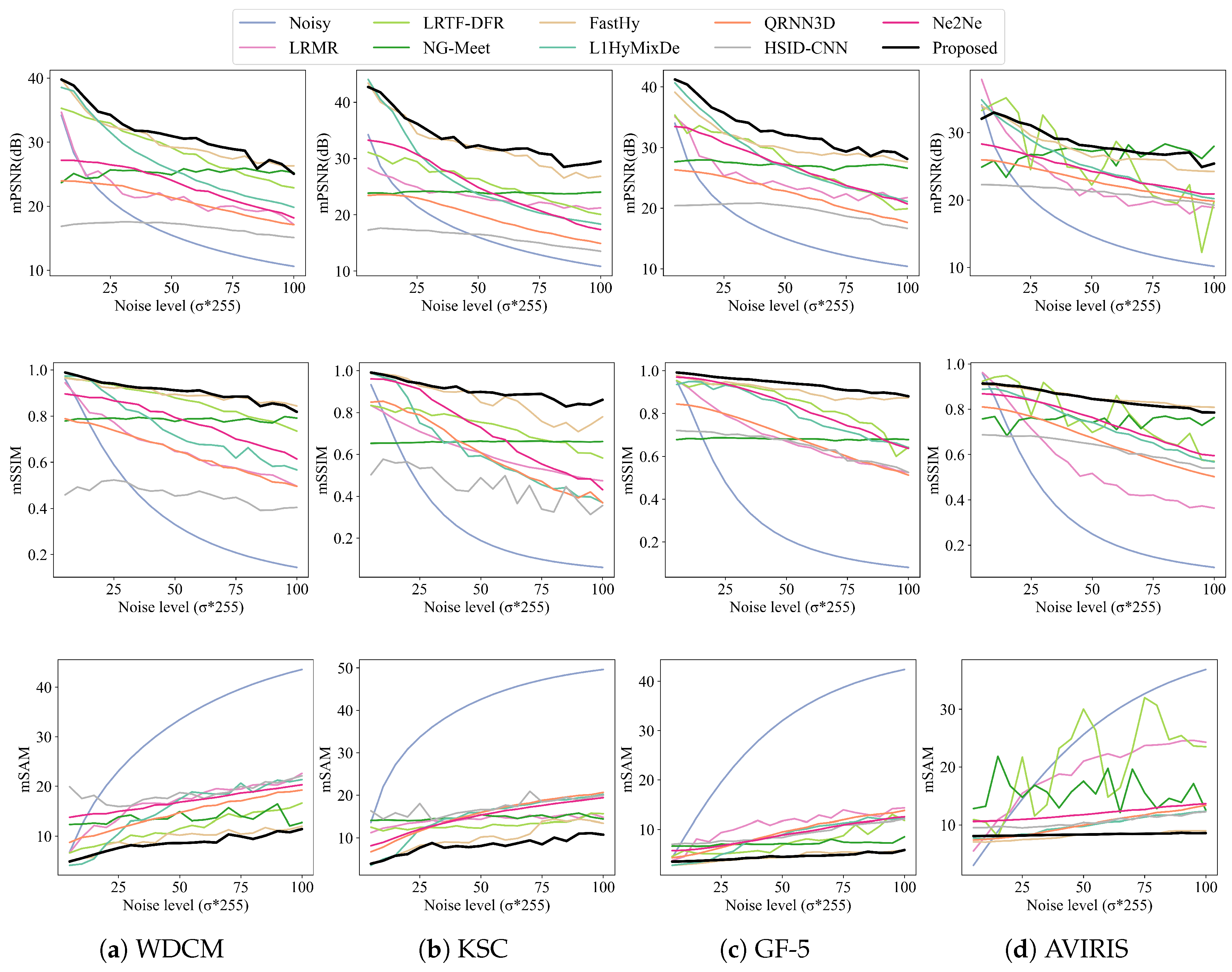
Figure 5.
Recovered spectral curves at (127,77) in KSC Case 2 for all comparison methods.
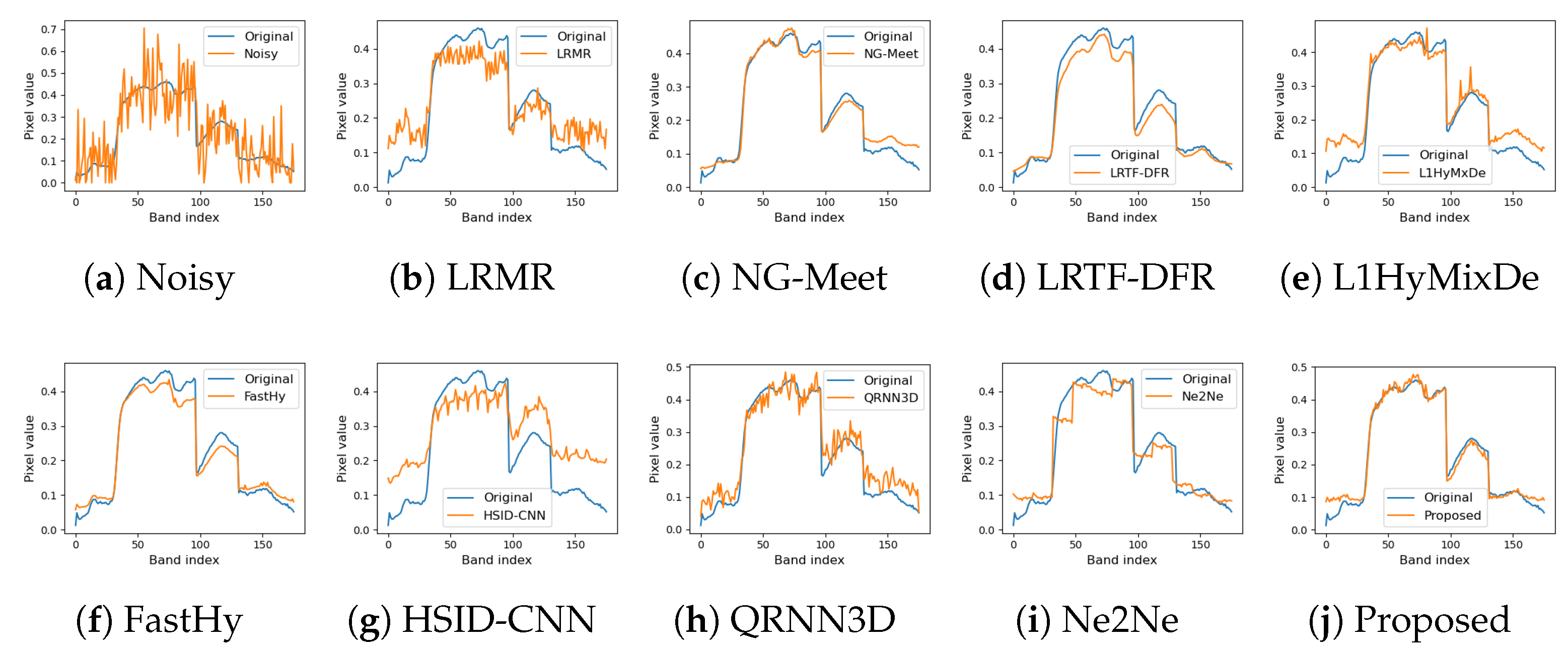
Figure 6.
Recovered spectral curves at (10,122) in AVIRIS Case 5 for all comparison methods.
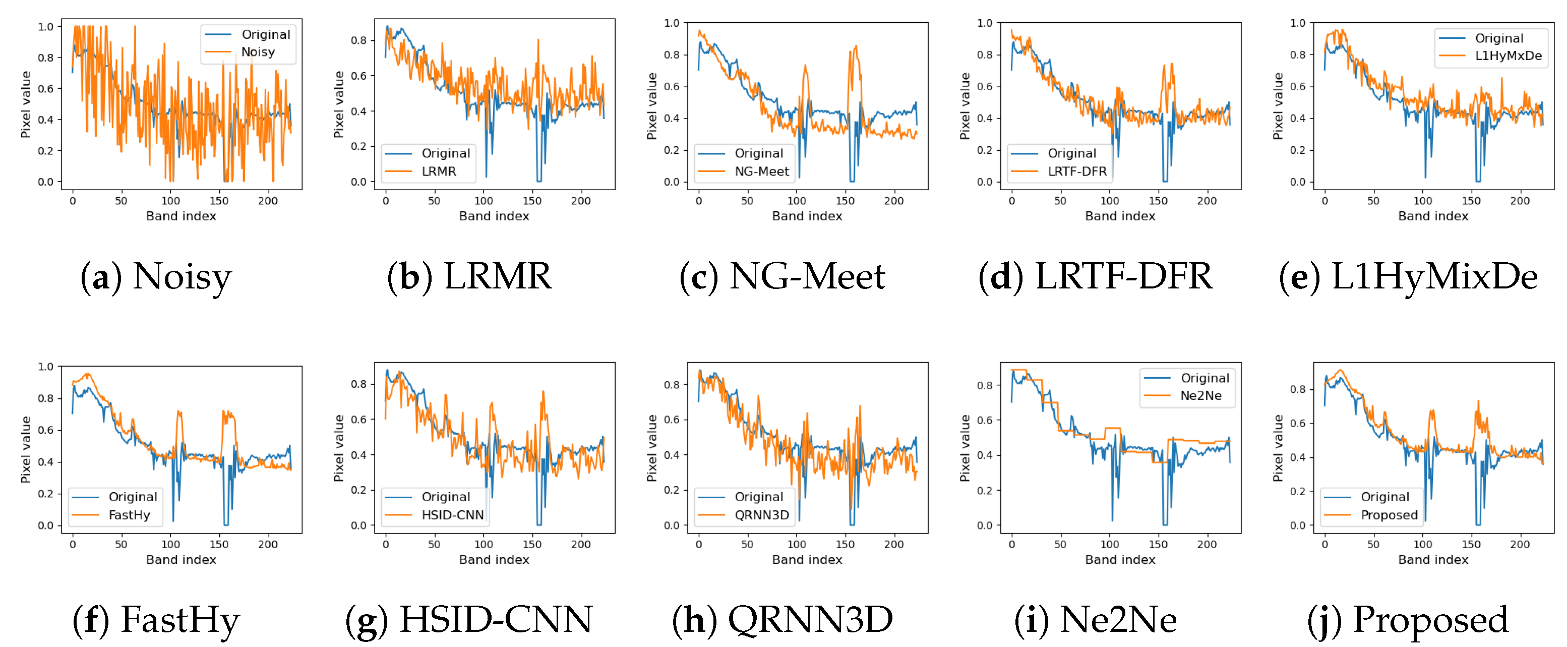
Figure 7.
Band 100 results of the simulated noise removal experiments on the WDCM dataset for Case 1-4 (from top to bottom).
Figure 7.
Band 100 results of the simulated noise removal experiments on the WDCM dataset for Case 1-4 (from top to bottom).

Figure 8.
Denoising results at band 100 of the KSC dataset for simulated cases 1–4 (from top to bottom).
Figure 8.
Denoising results at band 100 of the KSC dataset for simulated cases 1–4 (from top to bottom).

Figure 9.
The denoising results of WDCM, KSC, GF-5 and AVIRIS under Case 5 (from the first row to the fourth row). The Images displayed by different methods belong to different bands: band 111 of WDCM, 107 of KSC, 102 of GF-5 and 110 of AVIRIS.
Figure 9.
The denoising results of WDCM, KSC, GF-5 and AVIRIS under Case 5 (from the first row to the fourth row). The Images displayed by different methods belong to different bands: band 111 of WDCM, 107 of KSC, 102 of GF-5 and 110 of AVIRIS.
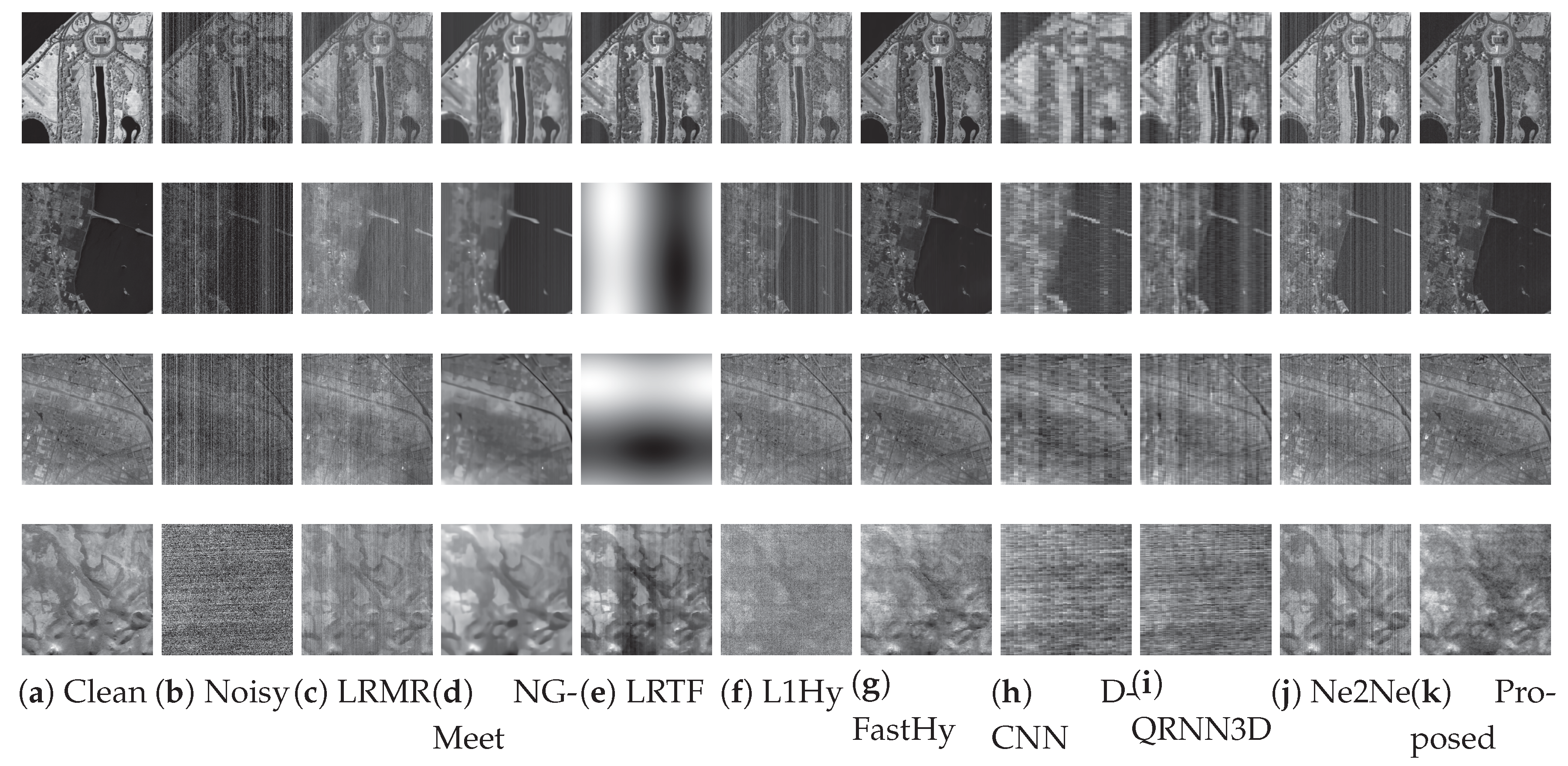
Figure 10.
The result of denoising experiment on 224th band of AVIRIS data and 330th band of GF-5 data.
Figure 10.
The result of denoising experiment on 224th band of AVIRIS data and 330th band of GF-5 data.
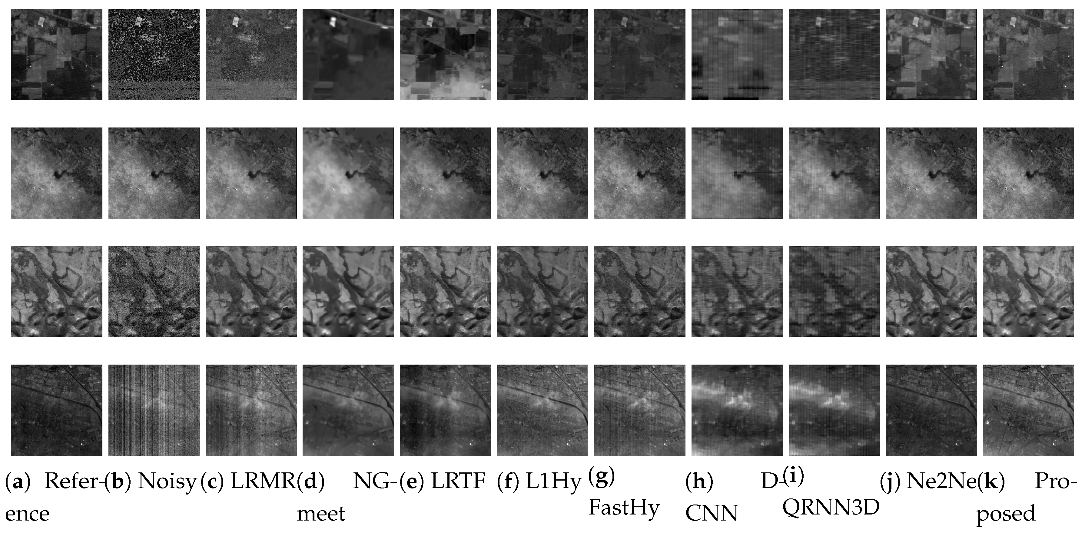
Figure 11.
Ablation study on ARSR and AWSSCLF.
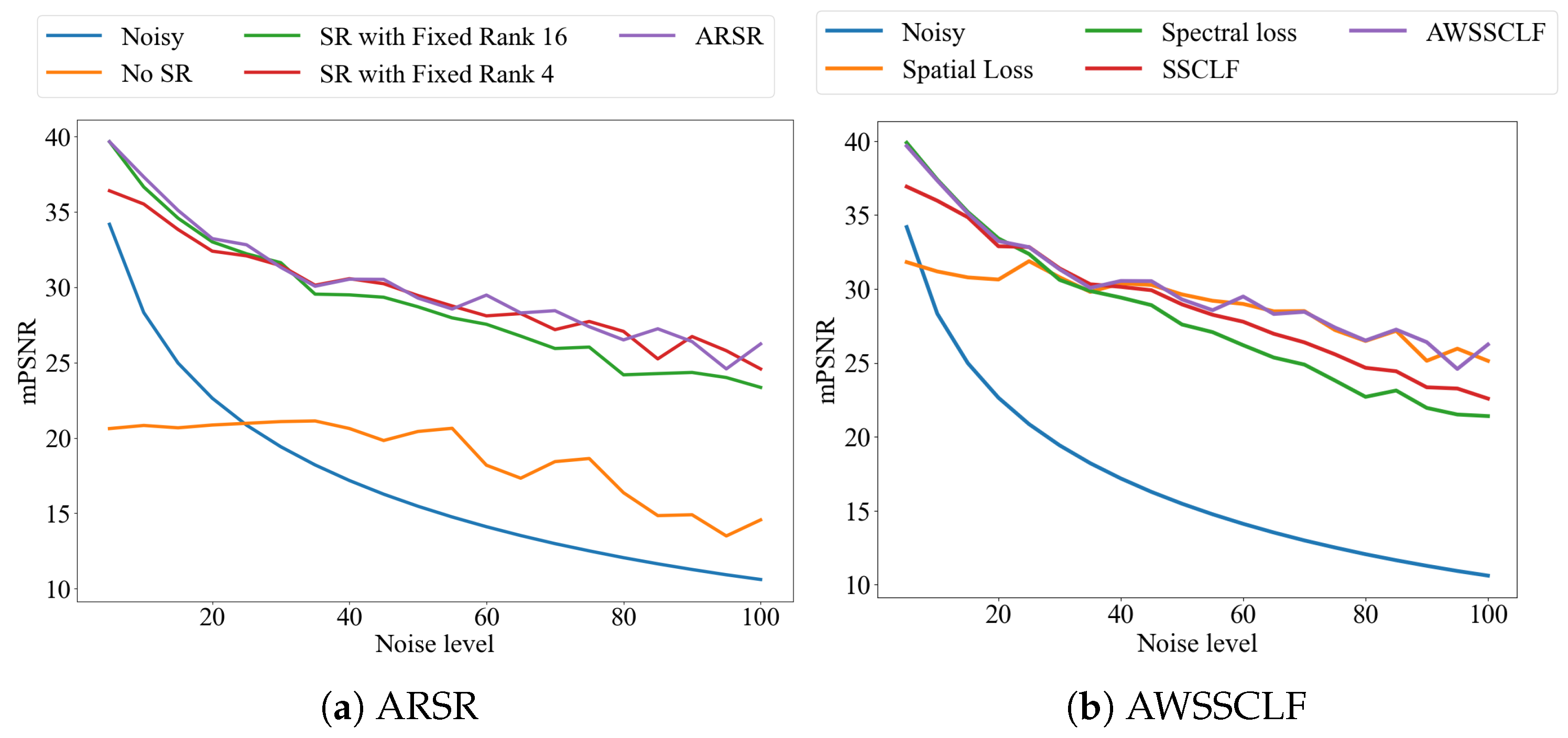
Figure 12.
Ablation study on network structure.
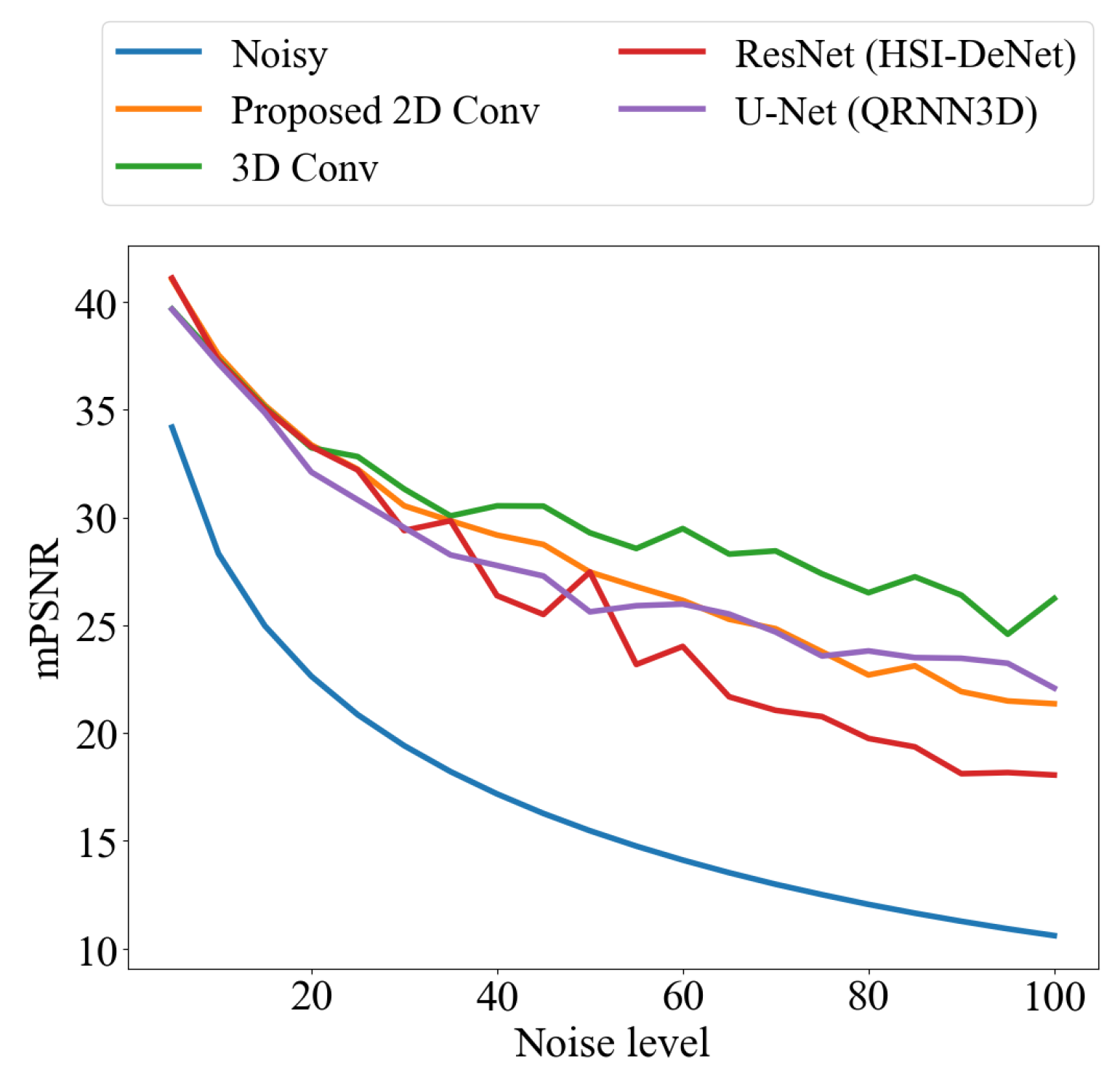
Figure 13.
The noise level estimation results of LAE, ADE and proposed SSHE, compared with the corresponding ground truth noise levels.
Figure 13.
The noise level estimation results of LAE, ADE and proposed SSHE, compared with the corresponding ground truth noise levels.
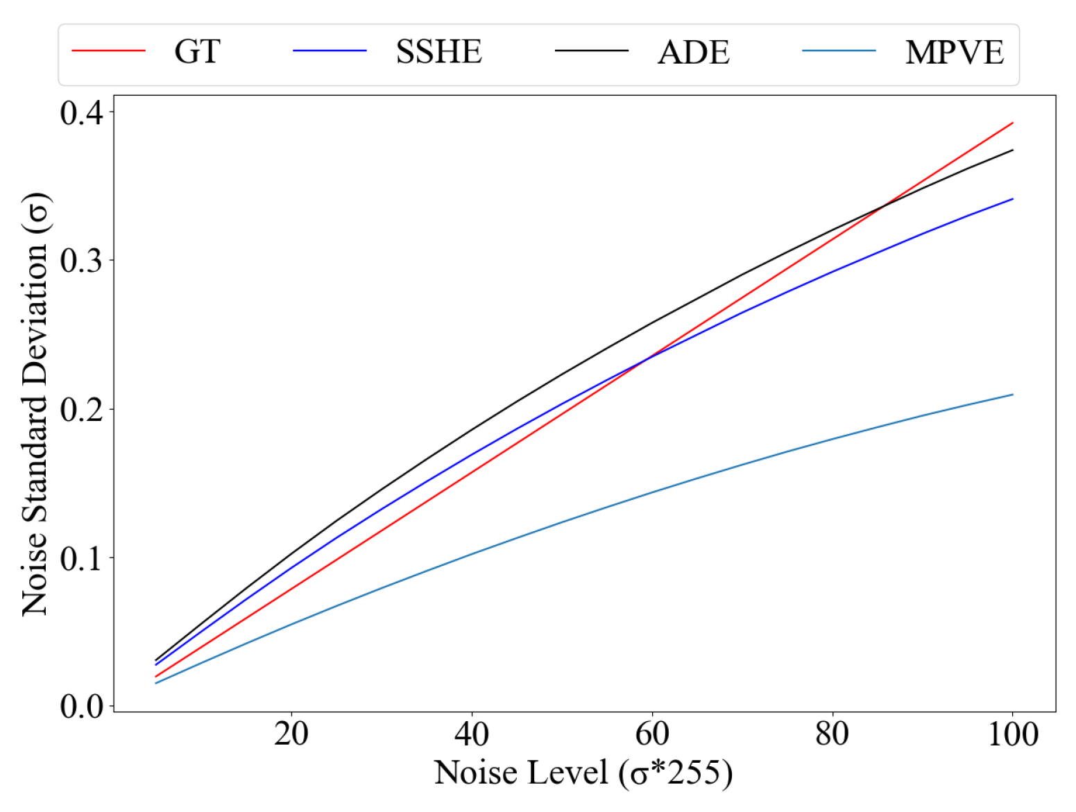

Table 1.
Quantitative comparison of all competing methods on the WDCM and KSC datasets. The best results are highlighted in bold
Table 1.
Quantitative comparison of all competing methods on the WDCM and KSC datasets. The best results are highlighted in bold
| Noisy | LRMR | NG-Meet | LRTF-DFR | L1HyMixDe | FastHy | HSID-CNN | Ne2Ne | QRNN3D | Proposed | ||
| WDCM | |||||||||||
| Case1 | mPSNR | 34.1996 | 33.1411 | 23.7342 | 34.6905 | 38.5335 | 39.6494 | 16.283 | 27.1649 | 23.9383 | 39.9849 |
| mSSIM | 0.9599 | 0.9547 | 0.8409 | 0.9763 | 0.9671 | 0.9578 | 0.4504 | 0.8958 | 0.7878 | 0.9890 | |
| mSAM | 6.7662 | 7.0999 | 12.3115 | 6.1528 | 4.7864 | 5.4596 | 19.8969 | 13.7181 | 8.6997 | 4.1058 | |
| Case2 | mPSNR | 20.8422 | 24.884 | 25.6972 | 32.1896 | 31.5029 | 32.5567 | 17.0672 | 26.458 | 23.2875 | 32.6666 |
| mSSIM | 0.588 | 0.842 | 0.8543 | 0.9655 | 0.8109 | 0.9237 | 0.4921 | 0.8656 | 0.7368 | 0.939 | |
| mSAM | 23.0836 | 12.6977 | 13.8343 | 7.1798 | 14.0855 | 8.0753 | 17.1872 | 14.9373 | 11.6199 | 9.3564 | |
| Case3 | mPSNR | 15.47 | 21.12 | 24.8601 | 28.9012 | 25.5963 | 29.4901 | 11.2258 | 24.0474 | 21.3145 | 29.4878 |
| mSSIM | 0.33 | 0.723 | 0.8388 | 0.9370 | 0.6985 | 0.8917 | 0.3262 | 0.7934 | 0.6498 | 0.9184 | |
| mSAM | 33.4264 | 17.8537 | 15.0978 | 8.713 | 18.0449 | 10.3574 | 26.1666 | 16.7844 | 14.7021 | 11.624 | |
| Case4 | mPSNR | 10.6074 | 18.9332 | 25.2726 | 22.7469 | 19.6676 | 24.9552 | 14.943 | 18.1661 | 17.1019 | 26.621 |
| mSSIM | 0.1441 | 0.6143 | 0.8553 | 0.821 | 0.5744 | 0.8554 | 0.4075 | 0.6139 | 0.4917 | 0.8595 | |
| mSAM | 43.5543 | 20.9286 | 12.7925 | 14.5153 | 21.012 | 11.1705 | 21.9956 | 20.2879 | 19.3081 | 13.2 | |
| Case5 | mPSNR | 15.3399 | 16.3694 | 18.6678 | 23.9983 | 24.6554 | 28.231 | 17.0409 | 20.1656 | 20.5653 | 28.9276 |
| mSSIM | 0.3263 | 0.5678 | 0.6655 | 0.8479 | 0.7183 | 0.8639 | 0.4658 | 0.6749 | 0.6348 | 0.9075 | |
| mSAM | 35.0802 | 23.6427 | 16.5209 | 14.3223 | 18.2969 | 15.236 | 19.2434 | 20.2184 | 17.2316 | 11.4248 | |
| KSC | |||||||||||
| Case1 | mPSNR | 34.2412 | 37.5316 | 24.9481 | 36.9613 | 44.3794 | 43.7204 | 16.9099 | 33.2468 | 23.2345 | 42.7613 |
| mSSIM | 0.9329 | 0.972 | 0.8409 | 0.9749 | 0.9866 | 0.9878 | 0.4704 | 0.9602 | 0.8398 | 0.9909 | |
| mSAM | 13.6064 | 6.507 | 12.6775 | 6.7717 | 3.8436 | 3.8184 | 17.0041 | 8.1344 | 6.9231 | 5.0374 | |
| Case2 | mPSNR | 21.4743 | 26.1399 | 26.6868 | 35.3979 | 31.3154 | 34.1601 | 16.7363 | 30.71 | 22.7779 | 34.5499 |
| mSSIM | 0.4508 | 0.7924 | 0.8491 | 0.9582 | 0.7784 | 0.9412 | 0.5544 | 0.9114 | 0.7852 | 0.9372 | |
| mSAM | 33.6641 | 14.2737 | 14.5205 | 8.6318 | 11.9604 | 7.8977 | 16.338 | 12.0228 | 11.5781 | 10.1316 | |
| Case3 | mPSNR | 16.023 | 19.9621 | 27.1994 | 31.6466 | 23.8516 | 32.2211 | 7.9278 | 24.8568 | 19.9464 | 30.0528 |
| mSSIM | 0.1887 | 0.5838 | 0.8286 | 0.9185 | 0.5954 | 0.8178 | 0.3016 | 0.7292 | 0.6069 | 0.9124 | |
| mSAM | 42.5897 | 21.2702 | 17.5872 | 12.2009 | 15.8523 | 11.6845 | 25.2886 | 15.306 | 15.9779 | 11.4229 | |
| Case4 | mPSNR | 10.8328 | 18.609 | 27.6856 | 25.6783 | 18.315 | 27.0152 | 13.2095 | 17.3612 | 14.9885 | 29.3451 |
| mSSIM | 0.06 | 0.4901 | 0.8503 | 0.8241 | 0.3877 | 0.7329 | 0.3617 | 0.4313 | 0.36 | 0.8716 | |
| mSAM | 49.6137 | 24.4529 | 13.2766 | 16.3273 | 20.0643 | 13.9542 | 19.7802 | 19.4100 | 20.7138 | 10.2948 | |
| Case5 | mPSNR | 16.026 | 16.0693 | 19.0167 | 7.3999 | 25.3434 | 30.5901 | 16.3794 | 19.9243 | 19.2514 | 28.1101 |
| mSSIM | 0.1945 | 0.4125 | 0.6323 | 0.3666 | 0.573 | 0.8818 | 0.4714 | 0.5315 | 0.6123 | 0.8503 | |
| mSAM | 43.1404 | 26.2597 | 18.1872 | 24.954 | 17.4208 | 12.58 | 17.8447 | 20.1234 | 17.7609 | 19.4106 | |
Table 2.
Quantitative comparison of all competing methods on the GF-5 and AVIRIS dataset. The best results are highlighted in bold
Table 2.
Quantitative comparison of all competing methods on the GF-5 and AVIRIS dataset. The best results are highlighted in bold
| Noisy | LRMR | NG-Meet | LRTF-DFR | L1HyMixDe | FastHy | HSID-CNN | Ne2Ne | QRNN3D | Proposed | ||
| GF-5 | |||||||||||
| Case 1 | mPSNR | 34.0356 | 35.6213 | 27.664 | 37.3411 | 40.794 | 38.876 | 19.8188 | 33.4585 | 26.2845 | 41.0434 |
| mSSIM | 0.9517 | 0.9735 | 0.827 | 0.9782 | 0.9376 | 0.9789 | 0.7178 | 0.9698 | 0.8401 | 0.9911 | |
| mSAM | 4.2508 | 3.6731 | 6.603 | 3.7652 | 2.7712 | 2.7818 | 7.0966 | 5.6999 | 4.2816 | 2.3931 | |
| Case 2 | mPSNR | 20.3603 | 26.2751 | 27.6737 | 33.1085 | 33.2365 | 32.6084 | 20.1893 | 30.742 | 25.2399 | 33.194 |
| mSSIM | 0.4774 | 0.8738 | 0.8313 | 0.9689 | 0.935 | 0.9412 | 0.6989 | 0.9379 | 0.7939 | 0.9653 | |
| mSAM | 19.5057 | 9.0891 | 6.8497 | 4.2081 | 4.8742 | 3.7523 | 7.7504 | 6.6756 | 6.3891 | 4.8609 | |
| Case 3 | mPSNR | 14.9915 | 23.6229 | 27.1764 | 28.0645 | 26.763 | 30.5307 | 12.7354 | 27.1525 | 22.907 | 29.6561 |
| mSSIM | 0.2149 | 0.7844 | 0.8259 | 0.9278 | 0.8095 | 0.9221 | 0.4424 | 0.8523 | 0.6931 | 0.9367 | |
| mSAM | 31.9724 | 11.9945 | 7.1674 | 6.9239 | 9.7997 | 4.5226 | 17.2469 | 8.8428 | 9.677 | 6.8598 | |
| Case 4 | mPSNR | 10.3989 | 21.5883 | 26.5495 | 19.3692 | 21.161 | 28.4796 | 16.5103 | 20.7051 | 17.7749 | 28.9979 |
| mSSIM | 0.0812 | 0.6731 | 0.8232 | 0.7256 | 0.6551 | 0.8748 | 0.5383 | 0.6371 | 0.508 | 0.8943 | |
| mSAM | 42.3827 | 14.1486 | 8.5733 | 12.0822 | 12.7367 | 5.7872 | 11.9243 | 12.517 | 13.8649 | 5.7200 | |
| Case 5 | mPSNR | 15.1019 | 19.8502 | 24.0653 | 8.5861 | 26.2542 | 30.238 | 20.1356 | 22.8616 | 22.1065 | 30.267 |
| mSSIM | 0.2214 | 0.6449 | 0.7414 | 0.4416 | 0.8503 | 0.8937 | 0.6682 | 0.7383 | 0.685 | 0.939 | |
| mSAM | 33.2 | 16.2035 | 10.0386 | 17.3323 | 10.2113 | 9.9385 | 10.3601 | 12.5154 | 12.011 | 6.3875 | |
| AVIRIS | |||||||||||
| Case 1 | mPSNR | 34.11 | 27.89 | 23.88 | 31.98 | 35.04 | 34.00 | 22.21 | 28.30 | 25.96 | 32.21 |
| mSSIM | 0.9571 | 0.8846 | 0.7772 | 0.9005 | 0.889 | 0.9072 | 0.6831 | 0.8681 | 0.8084 | 0.9136 | |
| mSAM | 3.0022 | 11.5702 | 13.8491 | 10.8137 | 7.6813 | 7.1497 | 9.6349 | 10.5819 | 7.3689 | 9.2551 | |
| Case 2 | mPSNR | 20.28 | 24.90 | 24.13 | 29.74 | 28.87 | 29.69 | 22.03 | 26.55 | 24.78 | 28.80 |
| mSSIM | 0.5183 | 0.7999 | 0.7789 | 0.8876 | 0.8428 | 0.886 | 0.679 | 0.8397 | 0.7659 | 0.8835 | |
| mSAM | 14.4262 | 13.9368 | 13.9948 | 11.599 | 8.2749 | 7.4654 | 9.5846 | 10.8997 | 8.1789 | 10.9115 | |
| Case 3 | mPSNR | 14.63 | 22.56 | 24.01 | 26.34 | 24.84 | 26.51 | 16.07 | 24.22 | 22.77 | 26.56 |
| mSSIM | 0.2495 | 0.7344 | 0.7809 | 0.8417 | 0.7354 | 0.8450 | 0.5191 | 0.7639 | 0.67 | 0.8451 | |
| mSAM | 25.587 | 14.5767 | 15.4063 | 12.9843 | 9.9279 | 8.3396 | 14.3058 | 11.7078 | 10.0134 | 13.7923 | |
| Case 4 | mPSNR | 10.15 | 20.89 | 24.03 | 19.63 | 20.30 | 24.57 | 19.13 | 20.90 | 19.79 | 25.40 |
| mSSIM | 0.102 | 0.6199 | 0.7795 | 0.7203 | 0.5683 | 0.8085 | 0.5531 | 0.5949 | 0.4991 | 0.7961 | |
| mSAM | 36.8718 | 15.1042 | 14.3703 | 16.6476 | 12.2839 | 8.9728 | 12.1489 | 13.6188 | 13.3766 | 14.15 | |
| Case 5 | mPSNR | 14.3825 | 20.338 | 21.4547 | 24.1274 | 24.0457 | 26.543 | 21.0976 | 21.8417 | 22.2976 | 26.5042 |
| mSSIM | 0.2551 | 0.6256 | 0.726 | 0.815 | 0.7237 | 0.808 | 0.6369 | 0.6732 | 0.6565 | 0.8423 | |
| mSAM | 27.5759 | 15.7701 | 17.0557 | 15.2223 | 12.4099 | 13.5277 | 11.8106 | 13.0086 | 13.2682 | 13.6372 | |
Table 3.
Ablation study: Component activation status
| Configuration * | ARSR | AWSSCLF | |||
| SR | DynRank | Spatial | Spectral | AdaptW | |
| Subspace Representation Studies | |||||
| NoSR | × | × | ✓ | ✓ | ✓ |
| Fixed rank-4 SR | ✓ | × | ✓ | ✓ | ✓ |
| Fixed rank-16 SR | ✓ | × | ✓ | ✓ | ✓ |
| ARSR | ✓ | ✓ | ✓ | ✓ | ✓ |
| Loss Function Studies | |||||
| Only spatial loss | ✓ | ✓ | ✓ | × | × |
| Only spectral loss | ✓ | ✓ | × | ✓ | × |
| SSCLF | ✓ | ✓ | ✓ | ✓ | × |
| AWSSCLF | ✓ | ✓ | ✓ | ✓ | ✓ |
* Legend: SR = Subspace Representation, DynRank = Dynamic Rank, AdaptW = Adaptive Weighted. : enabled, ×: disabled.
Disclaimer/Publisher’s Note: The statements, opinions and data contained in all publications are solely those of the individual author(s) and contributor(s) and not of MDPI and/or the editor(s). MDPI and/or the editor(s) disclaim responsibility for any injury to people or property resulting from any ideas, methods, instructions or products referred to in the content. |
© 2025 by the authors. Licensee MDPI, Basel, Switzerland. This article is an open access article distributed under the terms and conditions of the Creative Commons Attribution (CC BY) license (http://creativecommons.org/licenses/by/4.0/).
Copyright: This open access article is published under a Creative Commons CC BY 4.0 license, which permit the free download, distribution, and reuse, provided that the author and preprint are cited in any reuse.


