
Submitted:
21 August 2025
Posted:
25 August 2025
You are already at the latest version
Abstract
This study evaluated the seasonal variability of soil–atmosphere greenhouse gas (GHG) fluxes—carbon dioxide (CO₂), methane (CH₄), and nitrous oxide (N₂O)—across a land-use gradient in the Andean–Amazon transition zone of Colombia. The gradient included five land-use types incorporating at least one innovative climate-smart prac-tice—improved pasture (IP), cacao agroforestry system (CaAS), copoazu agroforestry system (CoAS), secondary forest with agroforestry enrichment (SFAE), and moriche palm swamp ecosystem (MPSE)—alongside the dominant regional land uses, old-growth forest (OF) and degraded pasture (DP). Soil GHG fluxes varied markedly among land-use types and between seasons. CO₂ fluxes were consistently higher during the dry season, whereas CH₄ and N₂O fluxes peaked in the rainy season. Agroecological and restoration systems exhibited substantially lower CO₂ emissions (7.34–9.74 Mg CO₂-C ha⁻¹ yr⁻¹) compared with DP (18.85 Mg CO₂-C ha⁻¹ yr⁻¹) during the rainy season, and lower N₂O fluxes (0.21–1.04 Mg CO₂-C ha⁻¹ yr⁻¹) during the dry season. In contrast, the MPSE presented high CH₄ emissions in the rainy season (300.45 kg CH₄-C ha⁻¹ yr⁻¹). Across all land uses, CO₂ was the dominant contributor to the total GWP (> 95% of emissions). The highest global warming potential (GWP) occurred in DP, whereas CaAS, CoAS and MPSE exhibited the lowest values. Soil temperature, pH, exchangeable acidity, texture, and bulk density play a decisive role in regulating GHG fluxes, whereas climatic factors, such as air temperature and relative humidity, influenced fluxes indirectly by modulating soil conditions. These findings underscore the role of diversified agroforestry and restoration systems in mit-igating GHG emissions and the need to integrate soil and climate drivers into regional climate models.
Keywords:
soil greenhouse gases
; land use change
; tropical agroforestry
; static chambers
; global warming potential
; soil temperature
; soil properties
; Andes-Amazon transition
1. Introduction
Carbon dioxide (CO2), methane (CH4), and nitrous oxide (N2O) are greenhouse gases (GHGs) present in the atmosphere that play a crucial role in regulating the Earth’s thermal balance and global climate [1]. These three gases contribute approximately 64%, 17%, and 6% of global GHG emissions, respectively [2,3]. Although CO2 has received considerable attention due to its increasing levels driven by human activities, CH4 has a global warming potential about 34 times greater, and N2O nearly 300 times greater than CO2 [4]. Consequently, accurate quantification of carbon sources and sinks is increasingly urgent to guide effective mitigation strategies [5].
Land-use change—particularly deforestation and the expansion of extensive cattle ranching—represents one of the main drivers of GHG emissions from terrestrial ecosystems in tropical regions [6]. Colombia lost 113,608 ha of forest in 2024, with deforestation concentrated mainly in the Amazon region (68%, 77,124 ha) and the Andes (13%, 14,910 ha). Notably, the Amazon experienced a 74% increase in deforestation (+32,850 ha) compared to 2023 [7]. Deforestation leads to a significant conversion of mature and secondary forests into pastures, often characterized by low productivity and poor soil management [8]. This process not only reduces carbon sequestration capacity but also increases soil degradation, biodiversity loss, and the likelihood of converting soils from GHG sinks into net sources [9]. Over the past 34 years, more than 3 million hectares have been cleared to make way for cattle ranching, making it the main driver of deforestation in Colombia’s Amazon (1985–2019 period) [10]. The livestock sector is a major emitter—accounting for 26% of Colombia’s total GHG emissions (258.8 Mt CO₂-eq year-1 in 2012). This accounted for 42% of AFOLU (Agriculture, Forestry and Other Land Use) sector emissions (158.6 Mt CO₂ eq yr⁻¹) [11]. This situation underscores the interconnections between extensive cattle ranching, forest loss, land degradation, and GHG emissions, positioning the Colombian Amazon as a key example for the transition from conventional production systems to sustainable, efficient, and resilient agroecological systems [12].
Natural ecosystems such forests (covering ~30% of Earth’s land surface), and wetlands (5–8% of land), play an essential role in regulating the global carbon cycle and mitigating climate change [13,14]. Wetlands foe example store between 20% and 30% of the planet’s soil carbon [15,16]. Pastures, covering about 40% of the terrestrial biosphere [17], may act as sinks for CO2 and CH4, as observed in natural savannas [18], but they can also become important sources of N2O under intensive use [19]. Meanwhile, agroecological production–restoration systems —such as organic and diversified agroforestry or secondary forests enriched with species of economic interest —are emerging as viable pathways to reconcile ecological integrity with productivity [20]. Such systems play a dual role as both sources and sinks [21,22]. Afforestation, for instance, can significantly reduce CO₂ emissions in former grasslands and deforested lands, as well as decrease CH₄ emissions across various intensive land uses [22]. However, the magnitude and direction of GHG fluxes from these systems—and their comparison with degraded pastures or natural ecosystems—remain poorly documented in many tropical transition landscapes.
The complexity of soil–atmosphere GHG exchanges requires an integrative approach that accounts for ecological attributes, soil physicochemical properties, and land management practices [23]. The magnitude of these fluxes is influenced by multiple factors, including soil moisture and temperature, land use, water table depth, precipitation, and soil properties such as pH, electrical conductivity, nutrient availability, and organic carbon content [24]. Land-use change and degradation can significantly alter the soil’s role as a source or sink [21,25].
Several studies have shown that GHG fluxes are also strongly modulated by topographic factors, microclimatic conditions, and land-use characteristics. Daniel et al. [26] noted that trees can act as filters or conduits for gases emitted from the soil, and that landscape position plays a significant role in regulating these fluxes across topographic gradients. Pang et al. [27] observed high spatial variability in N2O and CH4 fluxes, associated with heterogeneity in land use and canopy structure. Even small elevation differences can affect emission dynamics, as shown by Courtois et al. [28] in tropical soils. Lastly, Rajbonshi et al. [29] emphasized that changes in agricultural practices through agro-technological strategies can reduce GHG emissions, underlining the importance of climate-smart management in productive systems.
While global syntheses have shown that interactions between climate and soil variables are key drivers of the variability in soil GHG fluxes [23], fine-scale dynamics in heterogeneous landscapes—such as those of the Andes–Amazon Transition Zone—are far less understood. This gap limits the design of context-specific, climate-smart management strategies within the AFOLU sector.
In this context, we tested three main hypotheses: (1) we hypothesize that GHG fluxes vary significantly across land-use types, with lower emissions in systems that incorporate at least one innovative climate-smart agroecological practice relative to degraded pastures; (2) GHG fluxes show pronounced seasonal variability, with contrasting patterns between dry and rainy season depending on the type of gas; and (3) the magnitude and direction of GHG fluxes are primarily driven by interactions between soil physicochemical properties and climatic factors, with topography playing a secondary role.
This study aimed to assess variations in CO₂, CH₄, and N₂O fluxes across a land-use gradient in the Colombian Andes–Amazon Transition Zone, comparing land uses that incorporate at least one innovative climate-smart agroecological practice with the dominant land uses in the region, such as old-growth forests and degraded pastures. Our findings contribute to identifying emission patterns and drivers across this gradient, providing insights to guide the development of agroecological transitions toward agroecological food systems and bioeconomy-based economies (AEBE), with the potential to enhance competitiveness, productivity, resilience, and efficiency, while contributing to the achievement of Colombia’s NDC targets for climate change mitigation and adaptation in the AFOLU sectors.
2. Materials and Methods
2.1. Study Sites
The study was conducted in the department of Caquetá, in southern Colombia, within the transitional zone between the Andes mountain range and the Amazon region (Figure 1). The sampling area was located between 1°6′ and 1°30′ north latitude and 75°21′ and 76°9′ west longitude, encompassing representative areas of the municipalities of La Montañita, Belén de los Andaquíes, Albania, and San José del Fragua. This region is characterized by notable geomorphological heterogeneity, including alluvial plains, rolling hills, piedmonts, and mountainous areas [30]. The climate is classified as humid tropical, with a mean annual temperature of approximately 25 °C and an average annual precipitation of 3,235 mm. It follows a monomodal regime with two distinct seasons: a rainy season from March to June and a dry season from November to February [31]. According to USDA classification, the predominant soils are Inceptisols and Oxisols, which exhibit fine texture, poor drainage, high acidity (pH ranging from 4.5 to 5.8), high aluminum saturation, and low base saturation. These soils also present low levels of carbon, phosphorus, potassium, and magnesium, limiting their fertility and productive capacity [30].
2.2. Sampling Design
We selected seven land-use types: five that incorporated at least one form of innovative climate-smart agroecological practice—improved pasture (IP), cacao agroforestry system (CaAS), copoazu agroforestry system (CoAS), secondary forest with agroforestry enrichment (SFAE), and moriche palm swamp ecosystem (MPSE)—and two that represented the dominant land covers in the region—degraded pasture (DP) and old-growth forest (OF) (Supplementary Figure S1).
For each land-use type, five 20 × 30 m plots were purposively selected to ensure internal structural homogeneity in slope, soil type, canopy structure, and management history across the study sites, totaling 35 plots. Field data were collected during four campaigns in 2024, two in the dry season (January–February) and two in the rainy season (March–June), in order to capture seasonal variation in GHG fluxes.
Table 1 summarizes the main biophysical characteristics of the seven land-use types. IP sites were managed under rotational grazing schemes and included pasture subdivisions with species such as Brachiaria decumbes (Stapf) R.D. Webster, B. humidicola (Rendle) Schweick and B. brizantha cv. Marandú (A.Rich.) Stapf, complementary feeding systems such as mixed forage banks with species such as Pennisetum spp., Cratylia argentea (Desv.) Kuntze, Tithonia diversifolia (Hemsl.) A.Gray, and Piptocoma discolor (Kunth) Pruski, and liquid organic fertilization with pig-slurry digestate, representing a more sustainable livestock production model.
CaAS and CoAS sites represented biodiverse agroforestry systems with cacao (Theobroma cacao L.) and copoazu (Theobroma grandiflorum [Willd. ex Spreng.] Schum.), respectively, intercropped with native timber trees such as Cariniana pyriformis Miers, Cedrela odorata L., Minquartia guianensis Aubl., and Hevea brasiliensis (Willd. ex A. Juss.) Müll. Arg. These systems were established 10 to 14 years ago on lands historically used for temporary crops or pastures. Management practices relied exclusively on organic fertilization with vermicompost, avoided synthetic agrochemicals, and incorporated meliponiculture to enhance pollination services. Live barriers such as Chrysopogon zizanioides (L.) Roberty were established to minimize agrochemical drift from neighboring lands.
SFAE sites consisted of secondary forests aged 8–12 years, dominated by species such as Henriettea fascicularis (Sw.) M. Gómez, Miconia elata (Sw.) DC., Siparuna guianensis Aubl., and Cyathea lasiosora (Mett. ex Kuhn) Domin. These forests were enriched with native palms and fruit tree species such as Euterpe precatoria Mart., Oenocarpus bataua Mart., and T. grandiflorum, as well as windbreak trees including Cedrelinga cateniformis (Ducke) and M. guianensis, which had been established two years prior to sampling.
MPSE sites represented wetlands dominated by Mauritia flexuosa L.f., undergoing restoration through enrichment planting of native species (established two years prior to sampling), including M. guianensis, Virola elongata (Benth.) Warb., Aniba panurensis (Meisn.) Mez, C. cateniformis, Couma macrocarpa Barb.Rodr., E. precatoria, and O. bataua. These wetlands were further protected by livestock exclusion and subjected to minimal human disturbance.
DP sites were established on previously forested lands and have been used for over 15 years under extensive, traditional grazing. These areas are characterized by low cattle-carrying capacity, high soil compaction, and dominance of grasses such as Paspalum notatum Flüggé and Cynodon nlemfuensis Vanderyst (Bogdan).
OF sites corresponded to well-preserved natural forests, dominated by species such as Pseudosenefeldera inclinata (Müll.Arg.) Esser, Compsoneura capitellata (Poepp. ex A.DC.) Warb., Hymenaea oblongifolia Huber, Dialium guianense (Aubl.) Sandwith, Iriartea deltoidea Ruiz & Pav., Wettinia praemorsa (Willd.) Wess. Boer, Talisia cerasina (Benth.) Radlk, Calliandra surinamensis Benth., Licania harlingii Prance, C. odorata and Virola sebifera Aubl., with only minimal selective logging for household use, as previously reported [32].
Overall, site elevation ranged from 232 to 592 m a.s.l., while slope varied from 0.09° in flat pastures to 15.06° in steeper agroforestry areas. Soil organic carbon (SOC) stocks ranged between 48.13 and 73.57 Mg ha⁻¹ in DP and OF, respectively, whereas aboveground biomass carbon (AGBc) reached its highest levels in OF and MPSE (> 102 Mg C ha⁻¹), in sharp contrast with the low values recorded in DP (3.66 Mg C ha⁻¹).

Table 1.
Description of biophysical characteristics across the seven land-use types evaluated in the Andean–Amazon transition zone of Caquetá, Colombia.
Table 1.
Description of biophysical characteristics across the seven land-use types evaluated in the Andean–Amazon transition zone of Caquetá, Colombia.
| Biophysical characteristics | Plot | DP | IP | CaAS | CoAS | SFAE | MPSE | OF |
| Location | 1; 2; 3; 4; 5 | 1°17’23.86”N, 75°51’47.63”W; 1°11’52.36”N, 76°7’17.47”W; 1°23’05.44”N, 75°27’17.95”W; 1°09’17.09”N, 76°1’59.81”W; 1°18’52.70”N, 75°46’35.18”W | 1°11’53.48”N, 76°7’21.25”W; 1°11’53.47”N, 76°7’22.60”W; 1°17’11.06”N, 75°51’56.18”W; 1°17’09.24”N, 75°51’58.10”W; 1°20’27.08”N, 75°58’17.22”W | 1°16’07.23”N, 76°0’26.39”W; 1°16’06.61”N, 76°0’25.59”W; 1°22’01.17”N, 75°58’16.99”W; 1°09’03.09”N, 76°2’11.20”W; 1°09’02.43”N, 76°2’12.06”W | 1°15’42.87”N, 75°45’43.03”W; 1°15’42.88”N, 75°45’45.32”W; 1°15’32.21”N, 75°45’36.23”W; 1°15’31.80”N, 75°45’36.43”W; 1°18’23.39”N, 75°48’06.82”W | 1°14’46.03”N, 75°45’27.71”W; 1°14’47.40”N, 75°45’28.17”W; 1°18’59.81”N, 75°46’28.67”W; 1°17’25.37”N, 75°51’34.85”W; 1°16’02.59”N, 76°0’24.16”W | 1°22’52.60”N, 75°27’11.80”W; 1°22’54.04”N, 75°27’10.84”W; 1°23’04.84”N, 75°24’43.66”W; 1°23’01.37”N, 75°24’52.36”W; 1°22’59.61”N, 75°24’54.03”W | 1°11’50.71”N, 76°7’25.00”W; 1°11’49.66”N, 76°7’26.39”W; 1°17’31.99”N, 75°51’29.59”W; 1°18’49.95”N, 75°46’41.00”W; 1°15’27.55”N, 75°45’41.14”W |
| Elevation (m a.s.l.) | 1; 2; 3; 4; 5 | 265; 269; 232; 244; 254 | 323; 324; 268; 265; 414 | 367; 369; 592; 248; 244 | 242; 242; 242; 242; 264 | 242; 242; 254; 265; 367 | 232; 232; 242; 242; 242 | 323; 323; 256; 254; 242 |
| Slope (°) | 1; 2; 3; 4; 5 | 0.09; 2.27; 0.22; 0.29; 0.47 | 1.55; 1.55; 0.61; 0.61; 0.61 | 5.99; 5.99; 15.06; 0.29; 0.29 | 0.40; 0.40; 0.13; 0.13; 0.32 | 1.02; 1.02; 0.47; 0.24; 5.99 | 0.16; 0.16; 0.56; 0.23; 0.23 | 1.55; 2.91; 0.50; 0.33; 0.13 |
| Dominant species | P. notatum; C. nlemfuensis | B. descumbens; B. humidicola; B. brizantha | T. cacao; C. pyriformis; C. odorata; C. zizanioides | T. grandiflorum; C. pyriformis; M. guianensis; H. brasiliensis | H. fascicularis; M. elata; S. guianensis; C. lasiosora; T. grandiflorum; E. precatoria; O. Bataua; C. cateniformis; M. guianensis | M. flexuosa; M. guianensis, V. Elongata; A. Panurensis;, C. cateniformis C. macrocarpa; E. precatoria; O. bataua; | P. inclinata; C. capitellata, H. oblongifolia, D. Guianense, C. odorata, I. deltoidea; T. cerasina, C. surinamensis, L. Harlingii, W. praemorsa; V. sebifera | |
| Current land-use description | Degraded pastures under extensive grazing for over 15 years. | Pasture areas managed under rotational grazing systems for more than 15 years. | Agroforestry cacao systems with 10 to 14 years since planting. | Agroforestry copoazu systems with 10 to 14 years since planting. | Secondary forests aged 8–12 years, enriched with native palms and fruit tree species | Wetland areas predominantly colonized by M. flexuosa. | Natural forest areas that are relatively well-conserved, with limited selective logging primarily for household use. | |
| Land-use history | Previously secondary forest areas. | Previously secondary forest areas. | Previously secondary forest lands used for transitional crops (e.g., maize, plantain, cassava) and occasional grazing. | Areas previously used for pastures and/or secondary forests. | Previously used for pastures and subsistence crops. | Lightly disturbed wetlands. | Forests with minimal to moderate human activity, mainly associated with small-scale timber extraction. | |
| SOC (Mg ha-1) | 48.13 | 56.83 | 57.30 | 58.88 | 57.10 | 63.32 | 73.57 | |
| AGBc (Mg C ha-1) | 3.66 | 6.80 | 18.38 | 19.73 | 28.04 | 108.48 | 102.64 | |
DP = Degraded Pasture, IP = Improved Pasture, CaAS = Cacao Agroforestry System, CoAS = Copoazú Agroforestry System, SFAE = Secondary Forest with Agroforestry Enrichment, MPSE = Moriche Palm Swamp Ecosystem, OF = Old-Growth Forest. Location: geographic coordinates of the sampling plots; Elevation: elevation above sea level (m); Slope: terrain slope (°); Dominant species: most abundant tree and understory species observed per land use; Land-use description: current use characteristics and vegetation composition; Land-use history: previous land cover or use; SOC: soil organic carbon (Mg ha-1); AGBc: aboveground biomass carbon (Mg C ha-1).
2.3. Flux Measurements
In each sampling plot, a 15 m linear transect was established, within which three static polypropylene chambers were installed in a linear configuration, spaced 5 m apart. Each chamber consisted of a PVC collar (10 cm high, 20 cm in diameter) inserted 5 cm into the soil, and a matching PVC lid of the same dimensions as the collar, secured tightly with a rubber strap. The lid contained two rubber septa: one for inserting a digital punch thermometer (Full-Scale Traceable®® Thermometer, Traceable®®, USA) to record internal chamber temperature, and another for gas sampling using a 20 mL syringe connected to a three-way valve and an insulin needle. Collars were installed at least 24 h prior to gas collection to allow soil conditions to stabilize and minimize disturbance. Gas sampling was conducted between 9:00 a.m. and 3:00 p.m. to reduce diurnal variability in fluxes [26,28,33].
For each chamber, four gas samples were collected at 0, 15, 30, and 45 minutes after closure using pre-evacuated Labco Exetainer vials (5.9 mL, screw-cap), which were labeled with the sampling code, plot number, chamber ID, and sampling time. Beginning at minute 15, the chamber headspace was homogenized by gently pumping 15 mL of air in and out three times. Subsequently, 20 mL of gas were withdrawn; 5 mL were vented, and the remaining 15 mL were injected into the vial under pressure. One blank vial per plot was included to monitor ambient gas conditions.
Samples were carefully packaged and transported to the laboratory, where they were standardized by pressure equilibrium and subsequently analyzed using gas chromatography. CO₂ and CH₄ concentrations were determined with a flame ionization detector (FID) equipped with a methanizer, while N₂O concentrations were measured with an electron capture detector (ECD), both connected to a gas chromatograph (GC-2014, Shimadzu Corporation, Kyoto, Japan). The analytical conditions were as follows: column temperature of 80 °C; detector temperatures of 250 °C (FID) and 325 °C (ECD); methanizer temperature of 380 °C; 2 mL injection volume with an automatic loop; and nitrogen carrier gas flow of 30.83 mL min⁻¹. The limits of detection (LOD) and quantification (LOQ) were 0.0211 and 0.0704 ppm for CH₄, 37 and 125 ppm for CO₂, and 0.004 and 0.012 ppm for N₂O, respectively.
GHG fluxes were calculated in R using the gasfluxes package v.0.7 [34]. Gas concentrations (ppm) were converted to mass units using the ideal gas law and normalized to the surface area of each chamber. Four models were applied to each concentration time series: linear regression (LR), robust linear regression (RLR), Hutchinson–Mosier (HMR), and non-steady-state diffusion estimator (NDFE), allowing for an assessment of flux sensitivity under different statistical assumptions and concentration patterns [26,35,36]. The minimum detectable flux (MDF) for each gas was estimated following the procedure described by Parkin et al. [37], in order to identify and exclude values below the detection threshold. Most fluxes were estimated using RLR: 96.06% for CO2, 95.90% for CH4, and 95.71% for N2O, while the remaining values were calculated using LR. Fluxes below the detection limit were excluded from the analysis, corresponding to 6.73% of CO2, 15.33% of CH4, and 13.95% of N2O measurements.
2.4. Environmental Variables Measurements
During each sampling campaign, soil temperature (ST, °C) and volumetric water content (SWC, %) were recorded simultaneously with GHG flux measurements at a depth of 5 cm near the chambers. Both variables were measured with a portable sensor (TEROS 11, Decagon Devices, Pullman, WA, USA). In addition, three soil subsamples were randomly collected per plot and subsequently combined into a representative composite sample for each site. Soil samples were collected at a depth of 0–20 cm, coinciding with GHG flux measurements, and were processed in the laboratory for subsequent physicochemical analyses. The variables assessed included soil organic carbon (SOC, Mg ha-1), determined by the Walkley–Black dichromate oxidation method and converted following the methods of Nelson and Somers [38] and Batjes [39]. Soil pH and electrical conductivity (EC, dS m⁻¹) were assessed using the saturation paste and the conductometric method [40]. Cation exchange capacity (CEC, meq 100 g⁻¹) was determined by titration with 1 M NaOH, and base saturation (BS, %) was calculated as the sum of exchangeable base cations (Ca²⁺, Mg²⁺, K⁺, and Na⁺), divided by CEC [40]. Exchangeable acidity (EA) (mg kg−1) via 1N KCl volumetric method (NTC 5263) [71]. The percentages of sand, silt, and clay were estimated using the Bouyoucos method [40]. Available phosphorus (P, mg kg⁻¹) was determined using the Bray II method, and total nitrogen (N, %) content via the Kjeldahl method [40]. Bulk density (BD, g cm⁻³) was measured using a hand auger (Eijkelkamp Soil & Water, Giesbeek, The Netherlands).
Climatic and topographic variables were processed at the plot level using R v. 4.4.3 [41] and RStudio v. 2025.05.04 [42]. Daily meteorological data were retrieved from the NASA POWER platform using the get_power() function from the nasapower package [43], based on each plot’s geographic coordinates and the sampling dates. The extracted variables included air temperature at 2 meters (Temp, °C), relative humidity at 2 meters (RH, %), and precipitation on the day before sampling and over the five preceding days (Prec and Prec_5d, mm day-1) [44]. Elevation (m a.s.l.) was obtained from AWS Terrain Tiles using the elevatr package [45], from which a digital elevation model (DEM) with ~30 m resolution was also downloaded. Slope (in degrees) was derived from the DEM using the terrain() function in the terra package [46], and both elevation and slope values were extracted per plot using functions from the sf and terra packages.
2.5. Statistical Analysis
Linear mixed-effects models (LMMs) were fitted to assess the fixed effects of land-use types, season and their interactions on GHG fluxes using the lme function from the nlme v. 3.1-164 package [47] from R 4.4.3 [41], using the InfoStat v.2020 interface [48]. Plot was included as a random effect. The assumptions of normality and homoscedasticity were assessed through exploratory analysis of model residuals. To meet the normality requirement, CO₂ flux data were log-transformed, while CH₄ and N₂O fluxes were transformed using the formula log(flux − min(flux) + 1) [28]. To address heteroscedasticity across land-use types, a variance structure (varIdent) was applied [47]. Differences among fixed-effect means were evaluated through post hoc pairwise comparisons using Fisher’s LSD test (α = 0.05).
To assess the associations between gas fluxes and environmental factors (i.e., soil properties and climatic and topographic factors), pairwise Spearman correlation matrices were generated using the rcorr function in the Hmisc v. 5.1-3 R package [49]. The relationships between gas fluxes and the variables ST and SWC were further evaluated using simple linear regression with the lm function from the stats v. 4.3.3 R package [50]. Model evaluation was based on the coefficients of determination (R²) and residual diagnostics to assess goodness of fit. The resulting models were visualized using the ggplot2 v. 3.5.1 R package [51].
Structural equation models (SEMs) were used to examine the direct and indirect effects of environmental variables on each gas flux. The best SEMs were selected based on the Fisher’s C test and Akaike’s Information Criterion (AIC). SEMs were performed using the psem function from the piecewiseSEM v. 2.3.0 R package [52], and visualized with the grViz function from the DiagrammeR v. 1.0.11 R package [53]. All statistical analyses in R were conducted using the RStudio v.2025.05.0 interface [42].
3. Results
3.1. Soil CO2, CH4, and N2O Fluxes
Soil CO₂ fluxes varied significantly with land-use type (p < 0.001) and season (p < 0.01), with no significant interaction between these factors (p > 0.05) (Figure 2A; Supplementary Table S1). The highest average CO₂ emissions were recorded in DP (260.22 mg C m⁻² h⁻¹), followed by SFAE (188.02 mg C m⁻² h⁻¹), IP (184.43 mg C m⁻² h⁻¹) and OF (179.29 mg C m⁻² h⁻¹), whereas MPSE (98.59 mg C m⁻² h⁻¹), CaAS (108.76 mg C m⁻² h⁻¹), and CoAS (124.20 mg C m⁻² h⁻¹) exhibited the lowest mean values (Supplementary Figure S2A). Across seasons, higher mean fluxes were observed during the dry season (179.36 mg C m⁻² h⁻¹) compared with the rainy season (147.36 mg C m⁻² h⁻¹).
For CH₄, significant effects were observed for season (p < 0.001), land-use type (p < 0.001), and their interaction (p < 0.001) (Figure 2B; Supplementary Table S1). The highest average CH₄ emissions occurred in MPSE, with values of 3429.78 μg C m⁻² h⁻¹ during the rainy season and 1297.14 μg C m⁻² h⁻¹ in the dry season. In contrast, most other land uses acted as CH₄ sinks during the dry season, particularly OF (−48.25 μg C m⁻² h⁻¹), CoAS (−20.42 μg C m⁻² h⁻¹), DP (−14.25 μg C m⁻² h⁻¹), and IP (−8.74 μg C m⁻² h⁻¹). During the rainy season, the highest positive fluxes outside of MPSE were found in DP (150.57 μg C m⁻² h⁻¹) and IP (127.67 μg C m⁻² h⁻¹), followed by CoAS (13.94 μg C m⁻² h⁻¹) and SFAE (11.71 μg C m⁻² h⁻¹). Overall, MPSE exhibited the highest mean CH₄ flux (2363.46 μg C m⁻² h⁻¹), whereas CaAS (−0.47 μg C m⁻² h⁻¹), CoAS (−3.24 μg C m⁻² h⁻¹), and OF (−24.98 μg C m⁻² h⁻¹) showed the lowest mean values (Supplementary Figure S2B).
N₂O fluxes differed significantly by season (p < 0.01) and land-use type (p < 0.01), with no significant interaction between them (p > 0.05) (Figure 2C; Supplementary Table S1). Among land-use types, OF exhibited the highest mean N₂O flux (74.48 μg N m⁻² h⁻¹), followed by CaAS (30.54 μg N m⁻² h⁻¹), CoAS (18.42 μg N m⁻² h⁻¹), and SFAE (14.00 μg N m⁻² h⁻¹), whereas DP (13.64 μg N m⁻² h⁻¹), IP (9.11 μg N m⁻² h⁻¹), and MPSE (9.03 μg N m⁻² h⁻¹) showed the lowest mean values (Supplementary Figure S2C). Across seasons, mean fluxes were higher in the rainy season (30.79 μg N m⁻² h⁻¹) compared with the dry season (17.56 μg N m⁻² h⁻¹).
Figure 3 summarizes the differences and sums of means for each GHG across land-use types. Regarding the difference of mean fluxes (Figure 3A), a strong seasonal increase in CH4 emissions was observed in MPSE, with a positive difference of 2132.61 μg C m-2 h-1 between the rainy and dry seasons-by far the largest change recorded across all gases and land uses. Smaller increases were also observed in DP (163.38 μg C m-2 h-1) and IP (137.02 μg C m-2 h-1). For CO2, seasonal changes were negative across all land-use types, with the most marked reductions occurring in DP (-89.63 mg C m-2 h-1), CoAS (-28.14 mg C m-2 h-1), and OF (-28.94 mg m-2 h-1), indicating higher emissions during the dry season. In the case of N2O, seasonal differences were generally small, except for OF, which exhibited an increase of 45.26 μg N m-2 h-1 between seasons, while changes in other land uses remained below 13 μg N m-2 h-1.
Regarding the sum of mean fluxes (Figure 3B), MPSE again stood out with the highest total CH₄ emissions (4726.95 μg C m⁻² h⁻¹), far exceeding those from DP (136.33 μg C m⁻² h⁻¹) and all other land-use types. Cumulative CO₂ fluxes ranged from 198.83 mg C m⁻² h⁻¹ in MPSE to 520.00 mg C m⁻² h⁻¹ in DP, with intermediate values observed in IP (368.27 mg C m⁻² h⁻¹), SFAE (376.37 mg C m⁻² h⁻¹), and OF (359.09 mg C m⁻² h⁻¹). Regarding N₂O, although most land-use types exhibited relatively low cumulative fluxes, OF showed the highest value (149.08 μg N m⁻² h⁻¹), followed by CaAS (60.06 μg N m⁻² h⁻¹), CoAS (38.35 μg N m⁻² h⁻¹), and IP (17.20 μg N m⁻² h⁻¹), while SFAE recorded the lowest (24.54 μg N m⁻² h⁻¹).
When up-scaled from chamber-level measurements to annual plot-level estimates, soil GHG fluxes across land-use types and seasons revealed that CO₂ fluxes ranged from 7.34 Mg CO₂-C ha⁻¹ yr⁻¹ in MPSE during the rainy season to 26.70 Mg CO₂-C ha⁻¹ yr⁻¹ in DP during the dry season (Supplementary Table S2). CH₄ fluxes showed strong variability, with MPSE acting as the dominant source (113.63 and 300.45 kg CH₄-C ha⁻¹ yr⁻¹ in dry and rainy seasons, respectively), while most other land uses acted as sinks during the dry season (e.g., –4.23 kg CH₄-C ha⁻¹ yr⁻¹ in OF). N₂O fluxes were generally low, ranging from 0.21 kg N₂O-N ha⁻¹ yr⁻¹ in IP (dry season) to 8.51 kg N₂O-N ha⁻¹ yr⁻¹ in OF (rainy season).
3.2. Soil Temperature and Water Content
Both ST and SWC were significantly influenced by season, land-use type, and their interaction (Supplementary Table S1). During the dry season, the highest mean ST values were recorded in DP (27.89 °C), IP (27.48 °C), and CoAS (26.79 °C). In contrast, the lowest ST values were observed during the rainy season in CaAS ( 24.14 °C), followed by OF (24.32 °C) and CoAS (24.58 °C) (Figure 4A).
During the rainy season, the highest mean SWC values were recorded in MPSE (46.98%), CaAS (46.52%), and IP (45.10%), whereas in the dry season, the lowest values were observed in CoAS (39.38%), MPSE (39.72%), and SFAE (40.60%) (Figure 4B).
3.3. Environmental Drivers of Soil GHG Fluxes
Significant correlations were found between ST and N2O fluxes in both the dry and rainy season (both at p < 0.05), as well as with CH4 fluxes during the rainy season (p < 0.05). In contrast, SWC did not show significant associations with any gas in either season (p > 0.05) (Table 2). These relationships were supported by linear regressions models, where ST explained 37% of the variation in CO2 fluxes (R2 = 0.37, p < 0.001) and 18% in N2O fluxes (R2 = 0.18, p < 0.05), while its influence on CH₄ fluxes was weak (R2 = 0.03, p = 0.05). SWC did not significantly explain the variation in any GHG flux (R2 ranged from 0.002 to 0.04, p > 0.05) (Supplementary Figure S3).
The analysis of climatic, topographic, and physicochemical soil variables revealed marked differences among land-use types within each season (Supplementary Table S3). OF recorded the highest SOC values (86.47 Mg ha⁻¹) during the rainy season, whereas higher levels of N (0.19%), E_A (533.50 mg kg⁻¹), and silt content (20%) were observed in the dry season. CaAS showed the highest BS (47.99%) and clay content (48%) during the dry season, and the highest P (36.21 mg kg⁻¹) in the rainy season. BD was lowest in MPSE (0.99 g cm⁻³, rainy season), while the steepest slopes occurred in CaAS (7.11°) and SFAE (1.93°). Soil pH ranged from strongly acidic values in OF (3.94, dry season) to moderately acidic levels in CaAS (4.83, dry season). Temp and RH showed only minor variation among land-use types, whereas Prec prior to sampling peaked during the rainy season in SFAE (6.97 mm), with Prec_5d reaching its maximum in MPSE (43.61 mm).
The SEM for CO2 flux (R2 = 0.47) moderately explained the variability in CO2 emissions (Figure 5A). ST exerted the strongest and most significant direct effect on CO2 flux (standardized estimate = 0.65, p < 0.001), followed by RH which also showed a significant positive effect (0.36, p < 0.05). Although SOC and SWC were included as predictors, their direct effects were not statistically significant (p > 0.05). Indirectly, ST was determined by EC (-0.54, p < 0.001) and Temp (0.38, p < 0.01), while SWC was mainly influenced by BD (-0.32, p < 0.05), pH (0.37, p < 0.05), Temp (-0.41, p < 0.01), and RH (0.33, p < 0.05). The model presented a good overall fit (Fisher’s C = 20.91, p > 0.05).
The model for CH4 flux (R2 = 0.15) showed low explanatory power but an excellent global fit (Fisher’s C = 11.58, p > 0.05) (Figure 5B). Among all predictors, only ST showed a significant direct effect on CH4 emissions, with a negative relationship (-0.47, p < 0.05). The model highlighted relevant causal pathways for intermediate variables: E_A was positively influenced by CEC (0.75, p < 0.001) and negatively by pH (-0.33, p < 0.001), whereas SWC was determined by pH (0.41, p < 0.05) and Temp (-0.38, p < 0.05).
The model for N₂O flux (R² = 0.61) showed high explanatory capacity and an excellent fit (Fisher’s C = 4.58, p > 0.05) (Figure 5C). The most influential predictor of N₂O flux was EC (0.74, p < 0.001). EC was significantly affected by ST (−0.43, p < 0.01), pH (−0.30, p < 0.05), and SOC (0.38, p < 0.01). Although ST also had a positive direct effect on N₂O flux (0.17), this effect was not statistically significant (p > 0.05), nor were those of pH or P.
3.4. Global Warming Potential (GWP)
The global warming potential (GWP) derived from soil GHG fluxes varied considerably across land-use types (Table 3). DP exhibited the highest GWP values, with a seasonal average of 84.23 Mg CO2 eq ha-1 year-1, followed by IP (59.66 Mg CO2 eq ha-1 year-1) and SFAE (60.93 Mg CO2 eq ha-1 year-1). In contrast, MPSE showed the lowest mean GWP (39.83 Mg CO2 eq ha-1 year-1), along with CoAS (40.96 Mg CO2 eq ha-1 year-1) and CaAS (36.38 Mg CO2 eq ha-1 year-1). Overall, values were higher during the dry season than in the rainy season, particularly in DP (98.18 vs. 70.29 Mg CO2 eq ha-1 year-1). Although CH4 and N2O fluxes were included in the calculation, their combined contribution to total GWP was low (4.70 %), indicating that CO₂ was the dominant driver of the soil-derived climate impact.
4. Discussion
4.1. Contrasting GHG Fluxes Across Land-Use Types
GHG fluxes showed marked contrasts among different land-use types. DP exhibited the highest values, with a GWP of 84.23 Mg CO₂ eq ha⁻¹ yr⁻¹ and mean flux of 260.22 mg C m⁻² h⁻¹ as well as high values of ST. These high emissions in DP are linked to soil compaction, low vegetation cover, and a long history of extensive use—conditions that promote higher soil respiration rates by enhancing both microbial activity and the decomposition of surface organic matter [54]. This implies that degraded pastures not only present a negative carbon balance but also contribute significantly to the landscape’s GWP, underscoring the need to implement restoration and regenerative management practices aimed at recovering vegetation cover and improving soil physical properties [55,56]. In fact, our study found that IP had lower mean daily fluxes (184.43 mg C m⁻² h⁻¹) than DP, which is consistent with Soussana et al. [57], who highlight the key potential of integrated management practices to reduce the GHG balance in grazing systems. The conversion of forests to agricultural land, such as grasslands, tends to increase CO₂ and N₂O emissions. Degradation affects the soil’s ability to sequester carbon and alters biogeochemical cycles, resulting in higher GHG emissions [58].
In contrast, CaAS and CoAS agroforestry systems exhibited lower GWP values (36.38 and 40.96 Mg CO₂ eq ha⁻¹ yr⁻¹, respectively), with mean daily CO₂ fluxes not exceeding 138.16 mg C m⁻² h⁻¹ even during the dry season. This pattern suggests that tree cover and agroecological management practices in these systems help reduce thermal variability and direct soil exposure, thereby limiting carbon release to the atmosphere. This is consistent with Lemarpe et al. [59], who reported lower GHG fluxes in agroforestry systems compared to other land uses. The integrated functioning of vegetation and soil not only reduces net emissions but also contributes to key ecosystem services, such as soil biodiversity conservation, carbon sequestration, and water regulation, reinforcing the potential of agroforestry systems as nature-based strategies for climate change mitigation and adaptation [60,61].
MPSE stood out as the highest source of CH₄, with annual averages of 113.63 and 300.45 kg CH₄-C ha⁻¹ yr⁻¹ during the dry and rainy seasons, respectively. Emissions were particularly elevated in the rainy season, reaching peaks of 3429.78 µg C m⁻² h⁻¹, indicating the presence of stable anaerobic conditions that favored methanogenesis due to more intense waterlogging and low oxygen diffusion in the soil [62]. This behavior is consistent with observations in other tropical wetlands, where increases in temperature and water column height during flooding periods enhance CH₄ production and transport to the atmosphere [63,64,65,66]. Although MPSE exhibited net CH₄ emissions, their greater capacity to store carbon in biomass and soil (Table 1) offsets the impact of these fluxes on the system’s net carbon balance. From an ecological perspective, the role of wetlands in water regulation and carbon storage must be assessed alongside their sustained CH₄ emissions, so that GHG balances in landscapes that include them reflect their net contribution to the intensification of global warming [62,63].
OF recorded the highest N₂O emissions, with mean values of 8.51 kg N₂O-N ha⁻¹ yr⁻¹ during the rainy season and average fluxes of 74.48 µg N m⁻² h⁻¹. Also, acted as CH₄ sinks and had significant CO₂ emissions. These values were markedly higher compared to IP (9.11 µg N m⁻² h⁻¹) and DP (13.64 µg N m⁻² h⁻¹), which showed significantly lower means. These elevated values in OF are linked to the high availability of organic matter, enhanced microbial activity, and greater soil moisture during the rainy season, conditions that favor nitrification and denitrification processes, with N₂O released as a by-product [67,68], as well as the contribution of processes occurring in the litter layer [69,70]. These results are consistent with those of Mapanda et al. [58], who reported higher N₂O values in forests compared to plantations, grasslands, and croplands. Daniel et al. [26] reported that trees can act as filters for gases emitted from the soil and that their position in the landscape significantly influences the regulation of these flows. This could explain the high CO₂ flux values observed in OF.
4.2. Seasonal Variability of GHG Fluxes
Seasonal variation played a decisive role in the magnitude and pattern of GHG fluxes. CO₂ emissions were higher during the dry season across all land uses compared to the rainy season. These differences represented mean reductions of −32.87 mg C m⁻² h⁻¹, confirming that CO₂ emissions are greater under drier and warmer conditions, in which reduced soil moisture enhances oxygen diffusion and stimulates aerobic microbial activity, accelerating organic matter decomposition and consequently increasing CO₂ flux to the atmosphere [71]. Likewise, these findings are consistent with studies in tropical ecosystems where CO₂ pulses during dry periods reflect both microbial and root respiration, modulated by soil water availability and temperature [72,73]. In this context, the marked seasonality of CO₂ emissions implies that the annual carbon balance of tropical terrestrial systems is strongly conditioned by intra-annual climate variability, making them potentially more vulnerable to climate change scenarios in which the frequency and intensity of dry periods increase [74,75].
The seasonal increase in CH₄ emissions during the rainy season was particularly pronounced in MPSE, where emissions reached mean peaks of 3429.78 μg C m⁻² h⁻¹ in the rainy season compared to mean values of 1297.14 μg C m⁻² h⁻¹ in the dry season, representing a positive difference of 2132.61 μg C m⁻² h⁻¹ between the two periods. This result highlights the close relationship between hydrological dynamics and methane production in tropical environments, where prolonged soil saturation and reduced redox potential create anaerobic conditions that favor the activity of methanogenic communities, thereby significantly increasing CH₄ production and release [62]. In this context, the values recorded during the rainy season not only indicate intensified methanogenesis but also greater efficiency in gas transport to the atmosphere through diffusion and plant-mediated fluxes by flood-adapted species such as M. flexuosa [63,76]. In other land uses, an average increase of 65.51 μg C m⁻² h⁻¹ was observed during the rainy season, driven by higher soil moisture that inhibits CH₄ uptake [77].
For N₂O, an average increase of 12.44 μg N m⁻² h⁻¹ was observed during the rainy season. In fact, OF showed the highest increases during this period (46.53%), rising from 4.55 to 8.51 kg N₂O–N ha⁻¹ yr⁻¹. This pattern is consistent with studies reporting that the combination of prolonged water saturation and elevated temperatures promotes the formation of anoxic microsites, where denitrification is intensified, thereby enhancing N₂O production in tropical soils rich in organic matter and nitrogen [68,78,79,80]. Likewise, other studies have shown that such seasonal pulses can occur in response to internal nutrient recycling through litter decomposition and biological N fixation [81,82], and that their magnitude is related both to soil water saturation events and to the structure and functioning of the microbial community [83].
4.3. Environmental Drivers of GHG Fluxes
The analysis of environmental factors showed that ST was the main driver of CO₂ and N₂O emissions. The positive relationship between ST and CO₂ explained 37% of the observed variation, indicating that thermal increases accelerate heterotrophic respiration and organic matter decomposition, thereby enhancing carbon release from the soil to the atmosphere [84,85]. In contrast, the relationship between ST and N₂O was negative and accounted for 18% of the variation, suggesting that under warmer conditions, processes such as the reduction of N₂O to N₂ during complete denitrification may predominate, leading to lower net emissions of this gas [68,80]. Higher ST values were recorded in DP and IP during the dry season, whereas the lowest values occurred in CaAS and in OF during the rainy season. This marked thermal variability among land uses and seasons underscores the role of vegetation cover in regulating the soil microclimate and, consequently, in modulating GHG fluxes [86]. Therefore, our results suggest that strategies aimed at maintaining or increasing tree cover could buffer soil thermal extremes and potentially stabilize CO₂ and N₂O fluxes, contributing to climate-smart management of tropical landscapes [74,87].
SWC showed significant variations across seasons and land-use types. However, it did not exhibit significant associations with any of the gases, indicating that, under the evaluated conditions, water availability did not directly limit GHG production or consumption. Nevertheless, various studies have documented that soil moisture is a key controller of nitrification, denitrification, and methanogenesis, particularly in regions where shifts between aerobic and anoxic conditions generate pulses of N₂O and CH₄ [68,88]. In particular, sudden increases in soil water content following rainfall events can trigger ‘hot moments’ of emissions, driven by the rapid activation of microbial communities and shifts in substrate availability [89,90]. Therefore, although SWC variability did not directly control GHG fluxes in this study, its role could be more relevant under scenarios of greater water stress or during rapid transitions between moisture states, underscoring the importance of incorporating a broader range of agroclimatic conditions in future analyses.
The identification of soil physicochemical variables as key modulators of GHG fluxes underscores that emission dynamics in tropical ecosystems are determined by substrate availability, soil chemical status, and microbial activity. In the case of CO₂ flux, SOC did not exert a significant direct effect, but indirect pathways were evident through BD, pH, and EC (Figure 4). The fact that SOC exerts no direct effect on CO₂ but acts indirectly via properties such as pH, BD, and EC suggests that the quality and accessibility of carbon, rather than its total quantity, determine the intensity of soil respiration [84,85]. For N₂O, EC was the most influential predictor, itself dependent on SOC, pH, and ST. This relationship indicates that the concentration of dissolved salts and nutrients directly influences processes such as nitrification and denitrification, whose intensity and balance between gaseous products (N₂O and N₂) depend on pH, available organic carbon, and temperature [68,91]. Taken together, our results suggest that strategies aimed at conserving stable organic carbon, optimizing pH, and regulating salinity can mitigate N₂O emissions and stabilize CO₂ fluxes in tropical landscapes, supporting both adaptation and mitigation to climate change [87].
4.4. Global Warming Potential (GWP) Across Land-Use Types
CO₂ accounted for 95.30% of the total GWP, whereas CH₄ and N₂O, despite their high GWP per unit mass, jointly contributed only 4.70% due to their lower emission rates. This pattern is consistent with previous evidence indicating that heterotrophic and autotrophic respiration, sustained by high levels of organic matter and intense microbial activity, is the dominant source of emissions in soils with high productivity and rapid biomass turnover [27,84,85]. Therefore, our results underscores that although CH₄ and N₂O emissions must be considered due to their high warming potential, soil carbon dynamics and the processes regulating soil respiration have a disproportionate influence on the net climate balance of tropical landscapes. Consequently, mitigation strategies should prioritize actions that reduce soil carbon loss and maintain the carbon sequestration capacity of these systems [87].
The differences in GWP observed among the various land uses reflect the decisive role of vegetation cover and management practices in modulating net GHG emissions in tropical landscapes. The highest values were recorded in DP and IP, results consistent with previous studies indicating that the more intensive management practices typical of conventional systems, combined with lower canopy complexity, increase soil CO₂ emissions by elevating soil temperature and altering soil moisture dynamics [92,93]. In particular, the elevated GWP in SFAE and OF may be associated with the accumulation of litter and surface organic matter, which stimulate microbial activity and increase CO₂ and N₂O fluxes [69,94]. Conversely, the lowest values observed in agroforestry systems (CaAS, CoAS) and in ecosystems such as MPSE suggest that the presence of dense perennial vegetation, combined with conservation-oriented management, helps stabilize soil temperature and moisture, enhance organic carbon retention, and limit the accelerated mineralization of organic matter [28,87]. From a climate mitigation perspective, implementing strategies such as maintaining or increasing tree cover, reducing physical disturbance, improving nutrient recycling efficiency, and adopting practices such as zero tillage offers an effective pathway to lowering GWP and strengthening the resilience of tropical production systems to climate change [93,95]. Moreover, such diversification improves soil conditions [96] and enhances carbon storage [97].
5. Conclusions
This study demonstrated that soil GHG fluxes vary significantly among land-use types, with lower CO₂ and N₂O emissions in agroecological and restoration systems (i.e., land uses incorporating at least one innovative climate-smart agroecological practice) compared to degraded pastures. CO₂ was the dominant contributor to the total GWP, accounting for more than 95% of annual emissions. The highest GWP occurred in DP, whereas CaAS and CoAS, together with MPSE, exhibited the lowest values. CH₄ fluxes acted mainly as a sink in most land uses during the dry season but shifted to net emissions in MPSE during the rainy season. N₂O fluxes were more spatially localized, with OF recording the highest annual emissions, exceeding those observed in productive systems. Although higher emissions were measured in MPSE and OF, their greater capacity to store carbon in biomass and soil offsets these fluxes, maintaining a favorable net carbon balance.
Seasonal variability was evident and gas-specific: CO₂ fluxes peaked during the dry season, CH₄ shifted from a sink in most land uses during the dry season to a major source in MPSE during the rainy season, and N₂O fluxes showed limited seasonal variation, with localized peaks in OF. These patterns underscore the need for continuous, year-round monitoring to capture temporal dynamics.
Our results also highlight the decisive role of soil physicochemical properties—particularly soil temperature, pH, exchangeable acidity, texture, and bulk density—in regulating GHG fluxes, primarily through direct effects on CO₂, CH₄, and N₂O. Climatic factors such as air temperature and relative humidity influenced fluxes indirectly by modulating soil conditions, whereas topographic variables (elevation and slope) had no significant effect, suggesting that emission dynamics are more strongly controlled by soil quality and climatic variability than by landscape heterogeneity. Further studies are recommended to deepen the understanding of the interplay between soil physicochemical properties, soil water content, and GHG fluxes.
Overall, these findings demonstrate that diversified agroforestry and restoration-based land uses can substantially reduce soil-derived GHG emissions in deforested Andean–Amazonian landscapes. Integrating these systems into regional climate-smart strategies, while explicitly considering soil and climatic drivers in GHG modeling frameworks, may improve the accuracy of emission estimates, support effective mitigation policies, and foster agroecological transitions toward sustainable food systems and bioeconomy-based economies.
Supplementary Materials
The following supporting information can be downloaded at: Preprints.org, Figure S1. Representative photographs of the seven land-use types evaluated in the Andean–Amazon transition zone of Caquetá, Colombia; Figure S2. Soil GHG fluxes across seven land-use types (pooled across seasons) in the Andean–Amazon transition zone, Caquetá, Colombia; Figure S3. Linear regressions between soil GHG fluxes and soil variables measured simultaneously with the fluxes across land-use types in the Andean–Amazon transition zone, Caquetá, Colombia; Table S1. ANOVA results for season, land-use type, and their interaction on soil GHG fluxes, ST, and SWC in the Andean–Amazon transition zone, Caquetá, Colombia; Table S2. Annual soil GHG fluxes (mean ± SE) of CO₂ (Mg CO₂-C ha⁻¹ yr⁻¹), CH₄ (kg CH₄-C ha⁻¹ yr⁻¹), and N₂O (kg N₂O-N ha⁻¹ yr⁻¹) across seven land-use types and two seasons (dry and rainy) in the Andean–Amazon transition zone, Caquetá, Colombia; Table S3. Mean ± standard error of soil physicochemical, climatic and topographic variables across seven land-use types and two seasons (dry and rainy) in the Andean–Amazon transition zone, Caquetá, Colombia.
Author Contributions
Conceptualization, A.S., Y.D.S.-C., and N.A.R.-C.; methodology, A.S., Y.D.S.-C., and N.A.R.-C.; software, A.S.; validation, A.S.; formal analysis, A.S.; investigation, A.S., Y.D.S.-C., and N.A.R.-C.; resources, A.S. and C.H.R.-L.; data curation, Y.D.S.-C., and A.S.; writing—original draft preparation, A.S., and Y.D.S.-C.; writing—review and editing, A.S., Y.D.S.-C., N.A.R.-C. and C.H.R.-L.; visualization, A.S. and Y.D.S.-C.; supervision, A.S. and C.H.R.-L.; project administration, C.H.R.-L.; funding acquisition, C.H.R.-L. All authors have read and agreed to the published version of the manuscript.
Funding
This research was part of the project: “Fortaleciendo las capacidades territoriales para apoyar innovaciones en agroecología, pesca artesanal responsable y bioeconomía circular para la adaptación y mitigación al cambio climático en zonas costeras y fronteras forestales en Colombia DeSIRA (Development Smart Innovation through Research in Agriculture) 2020 – CO”, funded under the Subvención Acciones Exteriores FOOD/2021/423-487, through a contract between the European Union (EU) and the Instituto Amazónico de Investigaciones Científicas (SINCHI). The partner institutions include the Ministerio de Ciencia, Tecnología e Innovación (MINCIENCIAS), the Centre de Coopération Internationale en Recherche Agronomique pour le Développement (CIRAD), the Universidad Tecnológica del Chocó ‘Diego Luis Córdoba’ (UTCH), and the Corporación Colombiana de Investigación Agropecuaria (AGROSAVIA).
Institutional Review Board Statement
Not applicable.
Data Availability Statement
Data is contained within the article and Supplementary Materials.
Acknowledgments
The authors thank all the farmers in the study area for their help and support during the fieldwork.
Conflicts of Interest
The authors declare no conflicts of interest. The funders had no role in the design of the study; in the collection, analyses, or interpretation of the data; in the writing of the manuscript, or in the decision to publish the results.
References
- IPCC The Earth’s Energy Budget, Climate Feedbacks and Climate Sensitivity. In Climate Change 2021 – The Physical Science Basis; Cambridge University Press, 2023; pp. 923–1054.
- Tran, D.H.; Hoang, T.N.; Tokida, T.; Tirol-Padre, A.; Minamikawa, K. Impacts of Alternate Wetting and Drying on Greenhouse Gas Emission from Paddy Field in Central Vietnam. Soil Sci Plant Nutr 2018, 64, 14–22. [CrossRef]
- Myhre, G.; Shindell, D.; Bréon, F.-M.; Collins, W.; Fuglestvedt, J.; Huang, J.; Koch, D.; Lamarque, J.-F.; Lee, D.; Mendoza, B.; et al. Anthropogenic and Natural Radiative Forcing. In Climate Change 2013: The Physical Science Basis. Contribution of Working Group I to the Fifth Assessment Report of the Intergovernmental Panel on Climate Change; Stocker, T.F., Qin, D., Plattner, G.-K., Tignor, M., Allen, S.K., Boschung, J., Nauels, A., Xia, Y., Bex, V., Midgley, P.M., Eds.; Cambridge University Press: Cambridge, United Kingdom and New York, NY, USA., 2013.
- Chandrasekaran, D.; Tabassum-Abbasi; Abbasi, T.; Abbasi, S.A. Assessment of Methane Emission and the Factors That Influence It, from Three Rice Varieties Commonly Cultivated in the State of Puducherry. Atmosphere (Basel) 2022, 13, 1811. [CrossRef]
- IPCC Climate Change 2022 – Impacts, Adaptation and Vulnerability; Cambridge University Press, 2023; ISBN 9781009325844.
- FAO The State of the World’s Forests 2022. Forest Pathways for Green Recovery and Building Inclusive, Resilient and Sustainable Economies; FAO: Rome, Italy, 2022; ISBN 978-92-5-135984-6.
- Instituto de Hidrología, M. y E.A.-M. de A. y D.S. [Ideam-M. Actualización de Cifras de Monitoreo de La Superficie de Bosque - Año 2024. Resumen de Resultados de Monitoreo 2025; Bogota D.C., 2024.
- Agudelo-Hz, W.-J.; Castillo-Barrera, N.-C.; Uriel, M.-G. Scenarios of Land Use and Land Cover Change in the Colombian Amazon to Evaluate Alternative Post-Conflict Pathways. Sci Rep 2023, 13, 2152. [CrossRef]
- Bustamante, M.M.C.; Roitman, I.; Aide, T.M.; Alencar, A.; Anderson, L.O.; Aragão, L.; Asner, G.P.; Barlow, J.; Berenguer, E.; Chambers, J.; et al. Toward an Integrated Monitoring Framework to Assess the Effects of Tropical Forest Degradation and Recovery on Carbon Stocks and Biodiversity. Glob Chang Biol 2016, 22, 92–109. [CrossRef]
- Murillo-Sandoval, P.J.; Kilbride, J.; Tellman, E.; Wrathall, D.; Van Den Hoek, J.; Kennedy, R.E. The Post-Conflict Expansion of Coca Farming and Illicit Cattle Ranching in Colombia. Sci Rep 2023, 13, 1965. [CrossRef]
- IDEAM, P.M.D.C. Inventario Nacional y Departamental de Gases Efecto Invernadero – Colombia. Tercera Comunicación Nacional de Cambio Climático; Bogotá D.C, Colombia, 2016.
- Jiménez C, J.G.; Mantilla C, L.M.; Barrera G, J.A. Enfoque Agroambiental: Una Mirada Distinta a Las Intervenciones Productivas En La Amazonia. Caquetá y Guaviare.; Instituto SINCHI: Bogotá, Colombia, 2019; ISBN 2665-3451.
- Akande, O.J.; Ma, Z.; Huang, C.; He, F.; Chang, S.X. Meta-analysis Shows Forest Soil <scp> CO 2 </Scp> Effluxes Are Dependent on the Disturbance Regime and Biome Type. Ecol Lett 2023, 26, 765–777. [CrossRef]
- Feng, H.; Guo, J.; Peng, C.; Ma, X.; Kneeshaw, D.; Chen, H.; Liu, Q.; Liu, M.; Hu, C.; Wang, W. Global Estimates of Forest Soil Methane Flux Identify a Temperate and Tropical Forest Methane Sink. Geoderma 2023, 429, 116239. [CrossRef]
- Mitsch, W.J.; Gosselink, J.G. Wetlands; 5th ed.; John Wiley & Sons, Inc., 2015; ISBN 9781118676820.
- Mitsch, W.J.; Bernal, B.; Nahlik, A.M.; Mander, Ü.; Zhang, L.; Anderson, C.J.; Jørgensen, S.E.; Brix, H. Wetlands, Carbon, and Climate Change. Landsc Ecol 2013, 28, 583–597. [CrossRef]
- Liang, W.; Lü, Y.; Zhang, W.; Li, S.; Jin, Z.; Ciais, P.; Fu, B.; Wang, S.; Yan, J.; Li, J.; et al. Grassland Gross Carbon Dioxide Uptake Based on an Improved Model Tree Ensemble Approach Considering Human Interventions: Global Estimation and Covariation with Climate. Glob Chang Biol 2017, 23, 2720–2742. [CrossRef]
- Hörtnagl, L.; Barthel, M.; Buchmann, N.; Eugster, W.; Butterbach-Bahl, K.; Díaz-Pinés, E.; Zeeman, M.; Klumpp, K.; Kiese, R.; Bahn, M.; et al. Greenhouse Gas Fluxes over Managed Grasslands in Central Europe. Glob Chang Biol 2018, 24, 1843–1872. [CrossRef]
- Merbold, L.; Eugster, W.; Stieger, J.; Zahniser, M.; Nelson, D.; Buchmann, N. Greenhouse Gas Budget (CO 2 , CH 4 and N 2 O) of Intensively Managed Grassland Following Restoration. Glob Chang Biol 2014, 20, 1913–1928. [CrossRef]
- Rodríguez, C.; Sterling, A. Sucesión Ecológica y Restauración En Paisajes Fragmentados de La Amazonia Colombiana. Tomo 2. Buenas Prácticas Para La Restauración de Los Bosques; Instituto Amazónico de Investigaciones Científicas - SINCHI: Bogotá, DC. CO, 2021; ISBN 978-958-5427-28-0.
- He, T.; Ding, W.; Cheng, X.; Cai, Y.; Zhang, Y.; Xia, H.; Wang, X.; Zhang, J.; Zhang, K.; Zhang, Q. Meta-Analysis Shows the Impacts of Ecological Restoration on Greenhouse Gas Emissions. Nat Commun 2024, 15, 2668. [CrossRef]
- Liang, J.; Himes, A.; Siegert, C. A Meta-Analysis of Afforestation Impacts on Soil Greenhouse Gas Emissions. J Environ Manage 2025, 386, 125709. [CrossRef]
- Yan, W.; Zhong, Y.; Yang, J.; Shangguan, Z.; Torn, M.S. Response of Soil Greenhouse Gas Fluxes to Warming: A Global Meta-analysis of Field Studies. Geoderma 2022, 419, 115865. [CrossRef]
- Raturi, A.; Singh, H.; Kumar, P.; Chanda, A.; Raturi, A. Spatiotemporal Patterns of Greenhouse Gas Fluxes in the Subtropical Wetland Ecosystem of Indian Himalayan Foothill. Environ Monit Assess 2024, 196, 882. [CrossRef]
- Mapanda, F.; Mupini, J.; Wuta, M.; Nyamangara, J.; Rees, R.M. A Cross-ecosystem Assessment of the Effects of Land Cover and Land Use on Soil Emission of Selected Greenhouse Gases and Related Soil Properties in Zimbabwe. Eur J Soil Sci 2010, 61, 721–733. [CrossRef]
- Daniel, W.; Stahl, C.; Burban, B.; Goret, J.-Y.; Cazal, J.; Richter, A.; Janssens, I.A.; Bréchet, L.M. Tree Stem and Soil Methane and Nitrous Oxide Fluxes, but Not Carbon Dioxide Fluxes, Switch Sign along a Topographic Gradient in a Tropical Forest. Plant Soil 2023, 488, 533–549. [CrossRef]
- Pang, J.; Peng, C.; Wang, X.; Zhang, H.; Zhang, S. Soil-Atmosphere Exchange of Carbon Dioxide, Methane and Nitrous Oxide in Temperate Forests along an Elevation Gradient in the Qinling Mountains, China. Plant Soil 2023, 488, 325–342. [CrossRef]
- Courtois, E.A.; Stahl, C.; Van den Berge, J.; Bréchet, L.; Van Langenhove, L.; Richter, A.; Urbina, I.; Soong, J.L.; Peñuelas, J.; Janssens, I.A. Spatial Variation of Soil CO2, CH4 and N2O Fluxes Across Topographical Positions in Tropical Forests of the Guiana Shield. Ecosystems 2018, 21, 1445–1458. [CrossRef]
- Rajbonshi, M.P.; Mitra, S.; Bhattacharyya, P. Agro-Technologies for Greenhouse Gases Mitigation in Flooded Rice Fields for Promoting Climate Smart Agriculture. Environmental Pollution 2024, 350, 123973. [CrossRef]
- IGAC, I.G.A.C. Estudio General de Suelos y Zonificación de Tierras Departamento de Caquetá. Escala 1:100.000; Imprenta Nacional de Colombia: Bogotá, D. C., 2014; ISBN 978 958 8323 73-2.
- Murad, C.A.; Pearse, J. Landsat Study of Deforestation in the Amazon Region of Colombia: Departments of Caquetá and Putumayo. Remote Sens Appl 2018, 11, 161–171. [CrossRef]
- Rodríguez-León, C.H.; Sterling, A.; Daza-Giraldo, D.D.; Suárez-Córdoba, Y.D.; Roa-Fuentes, L.L. Scaling Plant Functional Strategies from Species to Communities in Regenerating Amazonian Forests: Insights for Restoration in Deforested Landscapes. Diversity (Basel) 2025, 17. [CrossRef]
- Pavelka, M.; Acosta, M.; Kiese, R.; Altimir, N.; Bruemmer, C.; Crill, P.; Darenova, E.; Fuß, R.; Gielen, B.; Graf, A.; et al. Standardisation of Chamber Technique for CO2, N2O and CH4 Fluxes Measurements from Terrestrial Ecosystems. Int Agrophys 2018, 32, 569–587. [CrossRef]
- Fuss, R. Gasfluxes: Greenhouse Gas Flux Calculation from Chamber Measurements. CRAN: Contributed Packages 2024.
- Pedersen, A.R.; Petersen, S.O.; Schelde, K. A Comprehensive Approach to Soil-Atmosphere Trace-Gas Flux Estimation with Static Chambers. Eur J Soil Sci 2010, 61, 888–902. [CrossRef]
- Hüppi, R.; Felber, R.; Krauss, M.; Six, J.; Leifeld, J.; Fuß, R. Restricting the Nonlinearity Parameter in Soil Greenhouse Gas Flux Calculation for More Reliable Flux Estimates. PLoS One 2018, 13, e0200876. [CrossRef]
- Parkin, T.B.; Venterea, R.T.; Hargreaves, S.K. Calculating the Detection Limits of Chamber-Based Soil Greenhouse Gas Flux Measurements. J Environ Qual 2012, 41, 705–715. [CrossRef]
- Nelson, D.W.; Sommers, L.E. Total Carbon, Organic Carbon, and Organic Matter. In Methods of Soil Analysis; SSSA Book Series; 1996; pp. 961–1010 ISBN 9780891188667.
- Batjes, N.H. Total Carbon and Nitrogen in the Soils of the World. Eur J Soil Sci 1996, 47, 151–163. [CrossRef]
- Soil Survey Staff Kellogg Soil Survey Laboratory Methods Manual. Soil Survey Investigations Report No. 42, Version 6.0. U.S; Lincoln, Nebraska, 2022.
- R Core Team R: A Language and Environment for Statistical Computing 2025.
- RStudio RStudio Version 2025.05.0 2025.
- Sparks, A. Nasapower: A NASA POWER Global Meteorology, Surface Solar Energy and Climatology Data Client for R. J Open Source Softw 2018, 3, 1035. [CrossRef]
- Mombrini, L.M.; de Mello, W.Z.; Ribeiro, R.P.; Silva, C.R.M.; Silveira, C.S. Physical and Hydric Factors Regulating Nitrous Oxide and Methane Fluxes in Mountainous Atlantic Forest Soils in Southeastern Brazil. J South Am Earth Sci 2022, 116, 103781. [CrossRef]
- Hollister, J.; Shah, T.; Nowosad, J.; Robitaille, A.L.; Beck, M.W.; Johnson, M. Elevatr: Access Elevation Data from Various APIs. CRAN: Contributed Packages 2023.
- Hijmans, R.J. Terra: Spatial Data Analysis. CRAN: Contributed Packages 2025.
- Pinheiro, J.; Bates, D.; DebRoy, S.; Sarkar, D. Nlme: Linear and Nonlinear Mixed Effects Models. R Package Version 3.1-131.1; 2018.
- Di Rienzo, J.A.; Casanoves, F.; Balzarini, M.G.; Gonzalez, L.; Tablada, M.; Robledo, C.W. InfoStat Versión 2020 2020.
- Harrell Jr, F.E. Hmisc: Harrell Miscellaneous. Version: 5.1-3. CRAN: Contributed Packages 2024.
- Worldwide, R.C.T. and contributors Package The R Stats Package Version 4.3.3. 2024.
- Wickham, H.; Chang, W.; Henry, L.; Pedersen, T.; Takahashi, K.; Wilke, C.; Woo, K.; Yutani, H. [aut]; Dunnington, D. Package ‘Ggplot2’: Create Elegant Data Visualisations Using the Grammar of Graphics Version 3.3.3. 2020.
- Rosseel, Y. Lavaan : An R Package for Structural Equation Modeling. J Stat Softw 2012, 48. [CrossRef]
- Iannone, R.; Roy, O. DiagrammeR: Graph/Network Visualization. Version: 1.0.11. CRAN: Contributed Packages 2024.
- Conant, R.T.; Cerri, C.E.P.; Osborne, B.B.; Paustian, K. Grassland Management Impacts on Soil Carbon Stocks: A New Synthesis. Ecological Applications 2017, 27, 662–668. [CrossRef]
- Follett, R.F.; Reed, D.A. Soil Carbon Sequestration in Grazing Lands: Societal Benefits and Policy Implications. Rangel Ecol Manag 2010, 63, 4–15. [CrossRef]
- Lal, R. Digging Deeper: A Holistic Perspective of Factors Affecting Soil Organic Carbon Sequestration in Agroecosystems. Glob Chang Biol 2018, 24, 3285–3301. [CrossRef]
- Soussana, J.F.; Tallec, T.; Blanfort, V. Mitigating the Greenhouse Gas Balance of Ruminant Production Systems through Carbon Sequestration in Grasslands. Animal 2010, 4, 334–350. [CrossRef]
- Mapanda, F.; Mupini, J.; Wuta, M.; Nyamangara, J.; Rees, R.M. A Cross-ecosystem Assessment of the Effects of Land Cover and Land Use on Soil Emission of Selected Greenhouse Gases and Related Soil Properties in Zimbabwe. Eur J Soil Sci 2010, 61, 721–733. [CrossRef]
- Lemarpe, S.E.; Musafiri, C.M.; Kiboi, M.N.; Ng’etich, O.K.; Macharia, J.M.; Shisanya, C.A.; Kibet, E.; Zeila, A.; Mutuo, P.; Ngetich, F.K. Smallholder Cropping Systems Contribute Limited Greenhouse Gas Fluxes in Upper Eastern Kenya. Nature-Based Solutions 2023, 4, 100098. [CrossRef]
- Ramachandran Nair, P.K.; Mohan Kumar, B.; Nair, V.D. Agroforestry as a Strategy for Carbon Sequestration. Journal of Plant Nutrition and Soil Science 2009, 172, 10–23. [CrossRef]
- Chauhan, S.; Kengoo, N.; Kishore, K.; Haksinhbhai, M.R.; Rana, P. Carbon Dynamics in Agroforestry Systems: Implications for Climate Change Mitigation and Adaptation. International Journal of Environment and Climate Change 2025, 15, 109–133. [CrossRef]
- Bridgham, S.D.; Cadillo-Quiroz, H.; Keller, J.K.; Zhuang, Q. Methane Emissions from Wetlands: Biogeochemical, Microbial, and Modeling Perspectives from Local to Global Scales. Glob Chang Biol 2013, 19, 1325–1346. [CrossRef]
- Sjögersten, S.; Black, C.R.; Evers, S.; Hoyos-Santillan, J.; Wright, E.L.; Turner, B.L. Tropical Wetlands: A Missing Link in the Global Carbon Cycle? Global Biogeochem Cycles 2014, 28, 1371–1386. [CrossRef]
- Bārdule, A.; Butlers, A.; Spalva, G.; Ivanovs, J.; Meļņiks, R.N.; Līcīte, I.; Lazdiņš, A. The Surface-to-Atmosphere GHG Fluxes in Rewetted and Permanently Flooded Former Peat Extraction Areas Compared to Pristine Peatland in Hemiboreal Latvia. Water (Basel) 2023, 15, 1954. [CrossRef]
- Castellón, S.E.M.; Cattanio, J.H.; Berrêdo, J.F.; Rollnic, M.; Ruivo, M. de L.; Noriega, C. Greenhouse Gas Fluxes in Mangrove Forest Soil in an Amazon Estuary. Biogeosciences 2022, 19, 5483–5497. [CrossRef]
- Cao, M.; Wang, F.; Ma, S.; Geng, H.; Sun, K. Recent Advances on Greenhouse Gas Emissions from Wetlands: Mechanism, Global Warming Potential, and Environmental Drivers. Environmental Pollution 2024, 355, 124204. [CrossRef]
- Werner, C.; Butterbach-Bahl, K.; Haas, E.; Hickler, T.; Kiese, R. A Global Inventory of N 2 O Emissions from Tropical Rainforest Soils Using a Detailed Biogeochemical Model. Global Biogeochem Cycles 2007, 21. [CrossRef]
- Butterbach-Bahl, K.; Baggs, E.M.; Dannenmann, M.; Kiese, R.; Zechmeister-Boltenstern, S. Nitrous Oxide Emissions from Soils: How Well Do We Understand the Processes and Their Controls? Philosophical Transactions of the Royal Society B: Biological Sciences 2013, 368, 20130122. [CrossRef]
- Jiang, J.; Wang, Y.-P.; Zhang, H.; Yu, M.; Liu, F.; Xia, S.; Yan, J. Contribution of Litter Layer to Greenhouse Gas Fluxes between Atmosphere and Soil Varies with Forest Succession. Forests 2022, 13, 544. [CrossRef]
- Duan, B.; Xiao, R.; Cai, T.; Man, X.; Ge, Z.; Gao, M.; Mencuccini, M. Strong Responses of Soil Greenhouse Gas Fluxes to Litter Manipulation in a Boreal Larch Forest, Northeastern China. Forests 2022, 13, 1985. [CrossRef]
- Bond-Lamberty, B.; Thomson, A. Temperature-Associated Increases in the Global Soil Respiration Record. Nature 2010, 464, 579–582. [CrossRef]
- Li, J.; Zhang, J.; Ma, T.; Lv, W.; Shen, Y.; Yang, Q.; Wang, X.; Wang, R.; Xiang, Q.; Lv, L.; et al. Responses of Soil Respiration to the Interactive Effects of Warming and Drought in Alfalfa Grassland on the Loess Plateau. Agronomy 2023, 13, 2992. [CrossRef]
- Wang, X.; Liu, L.; Piao, S.; Janssens, I.A.; Tang, J.; Liu, W.; Chi, Y.; Wang, J.; Xu, S. Soil Respiration under Climate Warming: Differential Response of Heterotrophic and Autotrophic Respiration. Glob Chang Biol 2014, 20, 3229–3237. [CrossRef]
- IPCC Climate Change 2021: The Physical Science Basis. Contribution of Working Group I to the Sixth Assessment Report of the Intergovernmental Panel on Climate Change. 2021.
- Wang, X.; Piao, S.; Ciais, P.; Friedlingstein, P.; Myneni, R.B.; Cox, P.; Heimann, M.; Miller, J.; Peng, S.; Wang, T.; et al. A Two-Fold Increase of Carbon Cycle Sensitivity to Tropical Temperature Variations. Nature 2014, 506, 212–215. [CrossRef]
- Pangala, S.R.; Enrich-Prast, A.; Basso, L.S.; Peixoto, R.B.; Bastviken, D.; Hornibrook, E.R.C.; Gatti, L. V.; Marotta, H.; Calazans, L.S.B.; Sakuragui, C.M.; et al. Large Emissions from Floodplain Trees Close the Amazon Methane Budget. Nature 2017, 552, 230–234. [CrossRef]
- Xu, N.; Li, J.; Zhong, H.; Wang, Y.; Dong, J.; Yang, X. Seasonal Dynamics of Greenhouse Gas Emissions from Island-like Forest Soils in the Sanjiang Plain: Impacts of Soil Characteristics and Climatic Factors. Forests 2024, 15, 996. [CrossRef]
- van Lent, J.; Hergoualc’h, K.; Verchot, L. V. Reviews and Syntheses: Soil N 2 O and NO Emissions from Land Use and Land-Use Change in the Tropics and Subtropics: A Meta-Analysis. Biogeosciences 2015, 12, 7299–7313. [CrossRef]
- Liu, H.; Zak, D.; Rezanezhad, F.; Lennartz, B. Soil Degradation Determines Release of Nitrous Oxide and Dissolved Organic Carbon from Peatlands. Environmental Research Letters 2019, 14, 094009. [CrossRef]
- Liptzin, D.; Rieke, E.L.; Cappellazzi, S.B.; Bean, G. Mac; Cope, M.; Greub, K.L.H.; Norris, C.E.; Tracy, P.W.; Aberle, E.; Ashworth, A.; et al. An Evaluation of Nitrogen Indicators for Soil Health in Long-term Agricultural Experiments. Soil Science Society of America Journal 2023, 87, 868–884. [CrossRef]
- Pereira, G.S.; Angnes, G.; Franchini, J.C.; Damian, J.M.; Cerri, C.E.P.; Rocha, C.H.; da Silva, R.V.; dos Santos, E.L.; Filho, J.T. Soil Nitrous Oxide Emissions after the Introduction of Integrated Cropping Systems in Subtropical Condition. Agric Ecosyst Environ 2022, 323, 107684. [CrossRef]
- Saha, D.; Basso, B.; Robertson, G.P. Machine Learning Improves Predictions of Agricultural Nitrous Oxide (N 2 O) Emissions from Intensively Managed Cropping Systems. Environmental Research Letters 2021, 16, 024004. [CrossRef]
- Peng, Y.; Wang, T.; Li, J.; Li, N.; Bai, X.; Liu, X.; Ao, J.; Chang, R. Temporal-Scale-Dependent Mechanisms of Forest Soil Nitrous Oxide Emissions under Nitrogen Addition. Commun Earth Environ 2024, 5, 512. [CrossRef]
- Davidson, E.A.; Janssens, I.A. Temperature Sensitivity of Soil Carbon Decomposition and Feedbacks to Climate Change. Nature 2006, 440, 165–173. [CrossRef]
- Bond-Lamberty, B.; Bailey, V.L.; Chen, M.; Gough, C.M.; Vargas, R. Globally Rising Soil Heterotrophic Respiration over Recent Decades. Nature 2018, 560, 80–83. [CrossRef]
- Powers, J.S.; Corre, M.D.; Twine, T.E.; Veldkamp, E. Geographic Bias of Field Observations of Soil Carbon Stocks with Tropical Land-Use Changes Precludes Spatial Extrapolation. Proceedings of the National Academy of Sciences 2011, 108, 6318–6322. [CrossRef]
- Rigon, J.P.G.; Calonego, J.C.; Pivetta, L.A.; Castoldi, G.; Raphael, J.P.A.; Rosolem, C.A. Using Cover Crops to Offset Greenhouse Gas Emissions from a Tropical Soil under No-Till. Exp Agric 2021, 57, 217–231. [CrossRef]
- Vargas, R.; Baldocchi, D.D.; Allen, M.F.; Bahn, M.; Black, T.A.; Collins, S.L.; Yuste, J.C.; Hirano, T.; Jassal, R.S.; Pumpanen, J.; et al. Looking Deeper into the Soil: Biophysical Controls and Seasonal Lags of Soil CO 2 Production and Efflux. Ecological Applications 2010, 20, 1569–1582. [CrossRef]
- Groffman, P.M.; Butterbach-Bahl, K.; Fulweiler, R.W.; Gold, A.J.; Morse, J.L.; Stander, E.K.; Tague, C.; Tonitto, C.; Vidon, P. Challenges to Incorporating Spatially and Temporally Explicit Phenomena (Hotspots and Hot Moments) in Denitrification Models. Biogeochemistry 2009, 93, 49–77. [CrossRef]
- Anthony, T.L.; Silver, W.L. Hot Moments Drive Extreme Nitrous Oxide and Methane Emissions from Agricultural Peatlands. Glob Chang Biol 2021, 27, 5141–5153. [CrossRef]
- Saggar, S.; Jha, N.; Deslippe, J.; Bolan, N.S.; Luo, J.; Giltrap, D.L.; Kim, D.-G.; Zaman, M.; Tillman, R.W. Denitrification and N2O:N2 Production in Temperate Grasslands: Processes, Measurements, Modelling and Mitigating Negative Impacts. Science of The Total Environment 2013, 465, 173–195. [CrossRef]
- Mühlbachová, G.; Růžek, P.; Kusá, H.; Vavera, R. CO2 Emissions from Soils under Different Tillage Practices and Weather Conditions. Agronomy 2023, 13, 3084. [CrossRef]
- Xing, Y.; Wang, X. Impact of Agricultural Activities on Climate Change: A Review of Greenhouse Gas Emission Patterns in Field Crop Systems. Plants 2024, 13, 2285. [CrossRef]
- Walkiewicz, A.; Rafalska, A.; Bulak, P.; Bieganowski, A.; Osborne, B. How Can Litter Modify the Fluxes of CO2 and CH4 from Forest Soils? A Mini-Review. Forests 2021, 12, 1276. [CrossRef]
- Li, T.; Lu, L.; Kang, Z.; Li, H.; Li, H. Warming Enhances Soil Microbial Respiration through Divergent Mechanisms in a Tropical Forest and a Temperate Forest. Geoderma 2025, 459, 117380. [CrossRef]
- Ngaba, M.J.Y.; Mgelwa, A.S.; Gurmesa, G.A.; Uwiragiye, Y.; Zhu, F.; Qiu, Q.; Fang, Y.; Hu, B.; Rennenberg, H. Meta-Analysis Unveils Differential Effects of Agroforestry on Soil Properties in Different Zonobiomes. Plant Soil 2024, 496, 589–607. [CrossRef]
- Warner, E.; Cook-Patton, S.C.; Lewis, O.T.; Brown, N.; Koricheva, J.; Eisenhauer, N.; Ferlian, O.; Gravel, D.; Hall, J.S.; Jactel, H.; et al. Young Mixed Planted Forests Store More Carbon than Monocultures—a Meta-Analysis. Frontiers in Forests and Global Change 2023, 6. [CrossRef]
Figure 1.
Study sites and distribution of sampling plots in the Andean–Amazon transition zone, Caquetá, Colombia. Land-use types: DP = Degraded Pasture, IP = Improved Pasture, CaAS = Cacao Agroforestry System, CoAS = Copoazu Agroforestry System, SFAE = Secondary Forest with Agroforestry Enrichment, MPSE = Moriche Palm Swamp Ecosystem, OF = Old-Growth Forest.
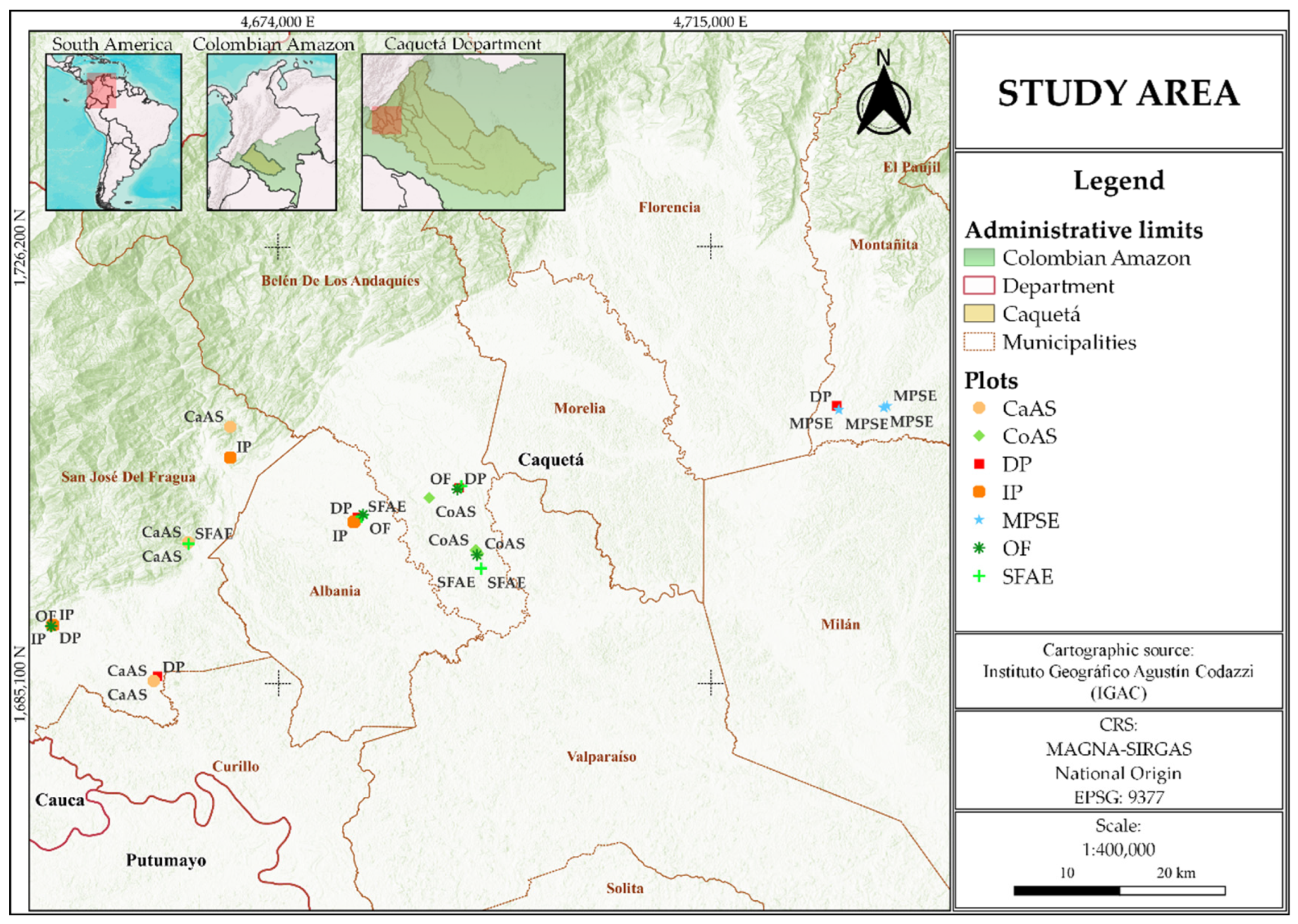
Figure 2.
Soil GHG fluxes across seven land-use types during two contrasting seasons in the Andean–Amazon transition zone, Caquetá, Colombia. Boxplots of CO₂ fluxes (mg C m⁻² h⁻¹) in (A), CH₄ fluxes (μg C m⁻² h⁻¹) in (B), and N₂O fluxes (μg N m⁻² h⁻¹) in (C), measured in degraded pasture (DP), improved pasture (IP), cacao agroforestry system (CaAS), copoazu agroforestry system (CoAS), secondary forest with agroforestry enrichment (SFAE), moriche palm swamp ecosystem (MPSE), and old-growth forest (OF) (n = 5). Orange and blue boxes represent measurements taken during the dry and rainy seasons, respectively. Different uppercase letters denote significant differences among land-use types (pooled across seasons), whereas lowercase letters indicate significant differences between seasons within the same land-use type (both at p < 0.05, Fisher’s LSD test). Boxes indicate interquartile ranges, horizontal lines represent medians, asterisks denote means, whiskers extend to data ranges, and dots indicate outliers.
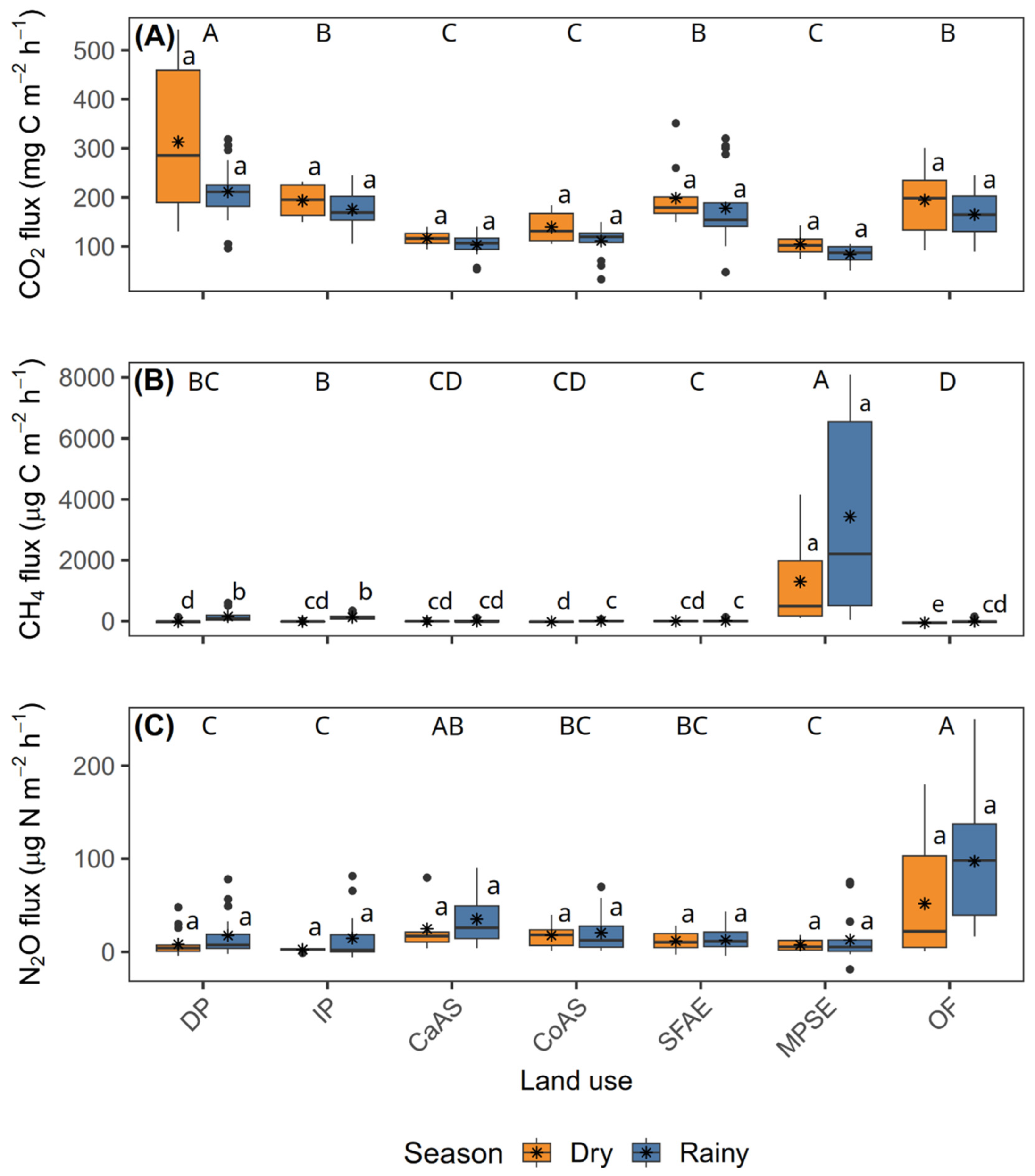
Figure 3.
(A) Difference in mean fluxes between rainy and dry seasons (Rainy – Dry) for CO2 (mg C m-2 h-1), CH4 (μg C m-2 h-1), and N2O (μg N m-2 h-1). Positive values indicate higher fluxes during the rainy season, while negative values reflect higher fluxes during the dry season. (B) Sum of mean fluxes during both seasons (Rainy + Dry), grouped by gas and land-use type. Bars are stacked by season to highlight relative seasonal contributions.
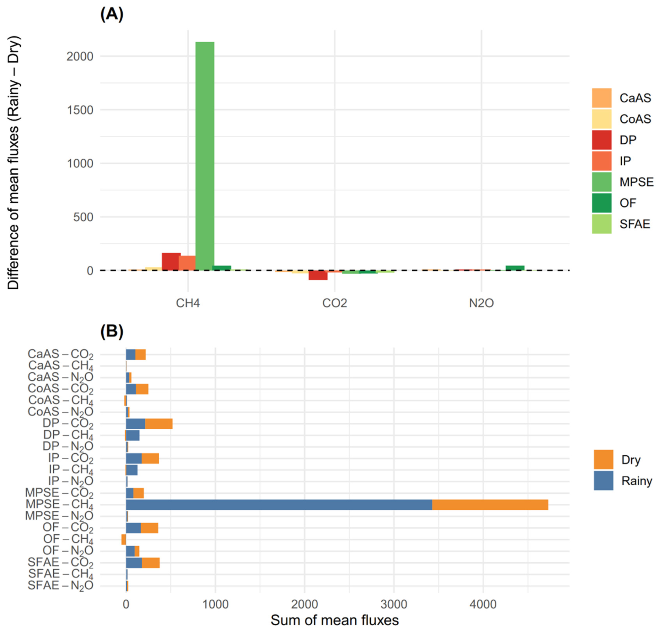
Figure 4.
Variation in soil temperature (ST, °C) and soil water content (SWC, %) across seven land-use types during two contrasting seasons in the Andean–Amazon transition zone, Caquetá, Colombia. Boxplots of ST in (A) and SWC in (B), measured in degraded pasture (DP), improved pasture (IP), cacao agroforestry system (CaAS), copoazu agroforestry system (CoAS), secondary forest with agroforestry enrichment (SFAE), moriche palm swamp ecosystem (MPSE), and old-growth forest (OF) (n = 5). Orange and blue boxes represent measurements taken during the dry and rainy seasons, respectively. Different uppercase letters denote significant differences among land-use types (pooled across seasons), whereas lowercase letters indicate significant differences between seasons within the same land-use type (both at p < 0.05, Fisher’s LSD test). Boxes indicate interquartile ranges, horizontal lines represent medians, asterisks denote means, whiskers extend to data ranges, and dots indicate outliers.
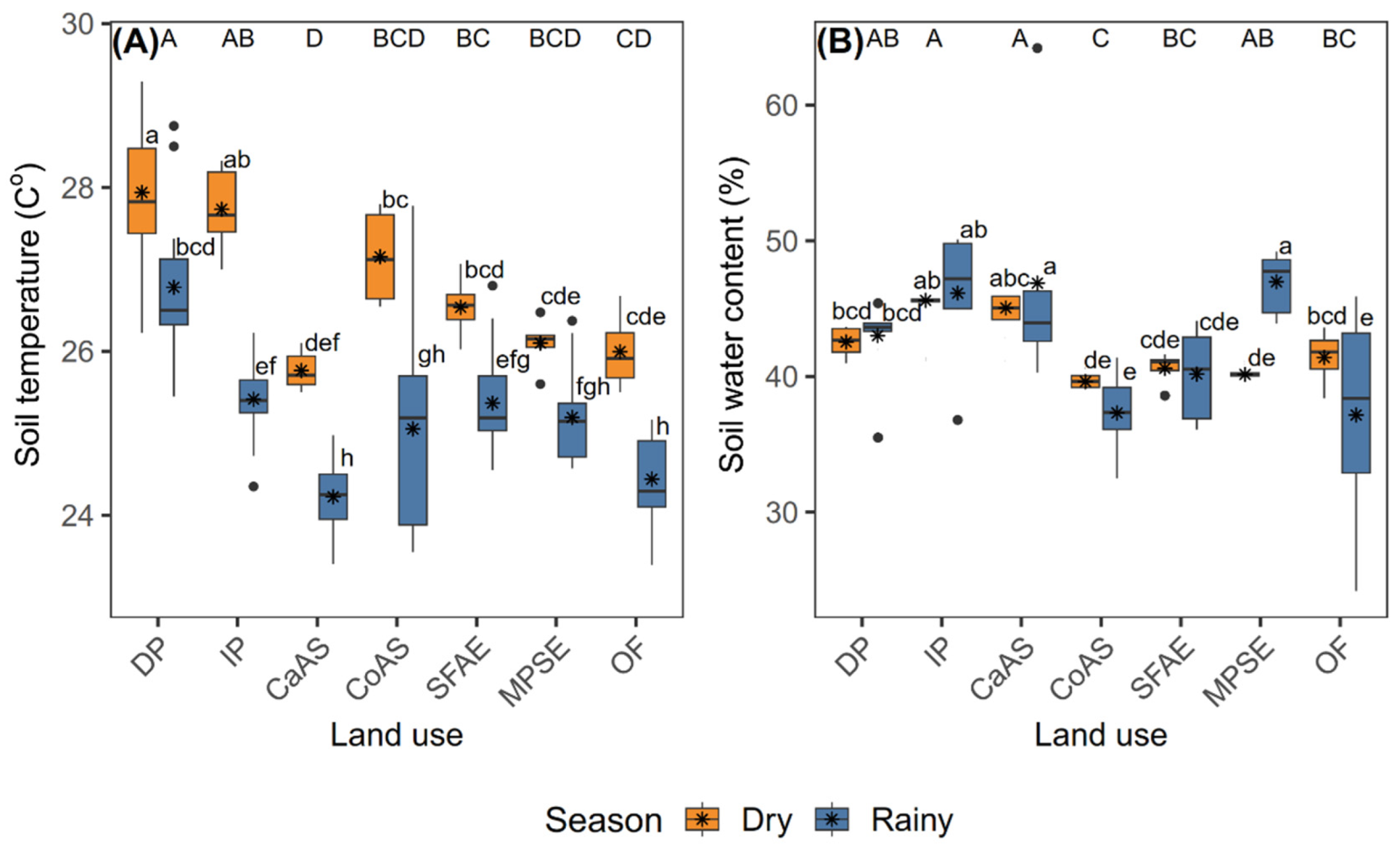
Figure 5.
Structural equation models (SEMs) depicting the direct and indirect relationships between environmental variables and soil GHG fluxes across different land-use types in the Andean–Amazon transition zone, Caquetá, Colombia. (A) Model for CO2 flux (mg C m-2 h-1), (B) for CH4 flux (μg C m-2 h-1), and (C) for N2O flux (μg N m-2 h-1). Arrows represent causal pathways, with green indicating positive effects and red negative effects. Path coefficients are standardized and shown along each arrow. Asterisks denote significance levels (* p < 0.05; ** p < 0.01; *** p < 0.001). R2 values indicate the proportion of variance explained for predictor variables in each model.
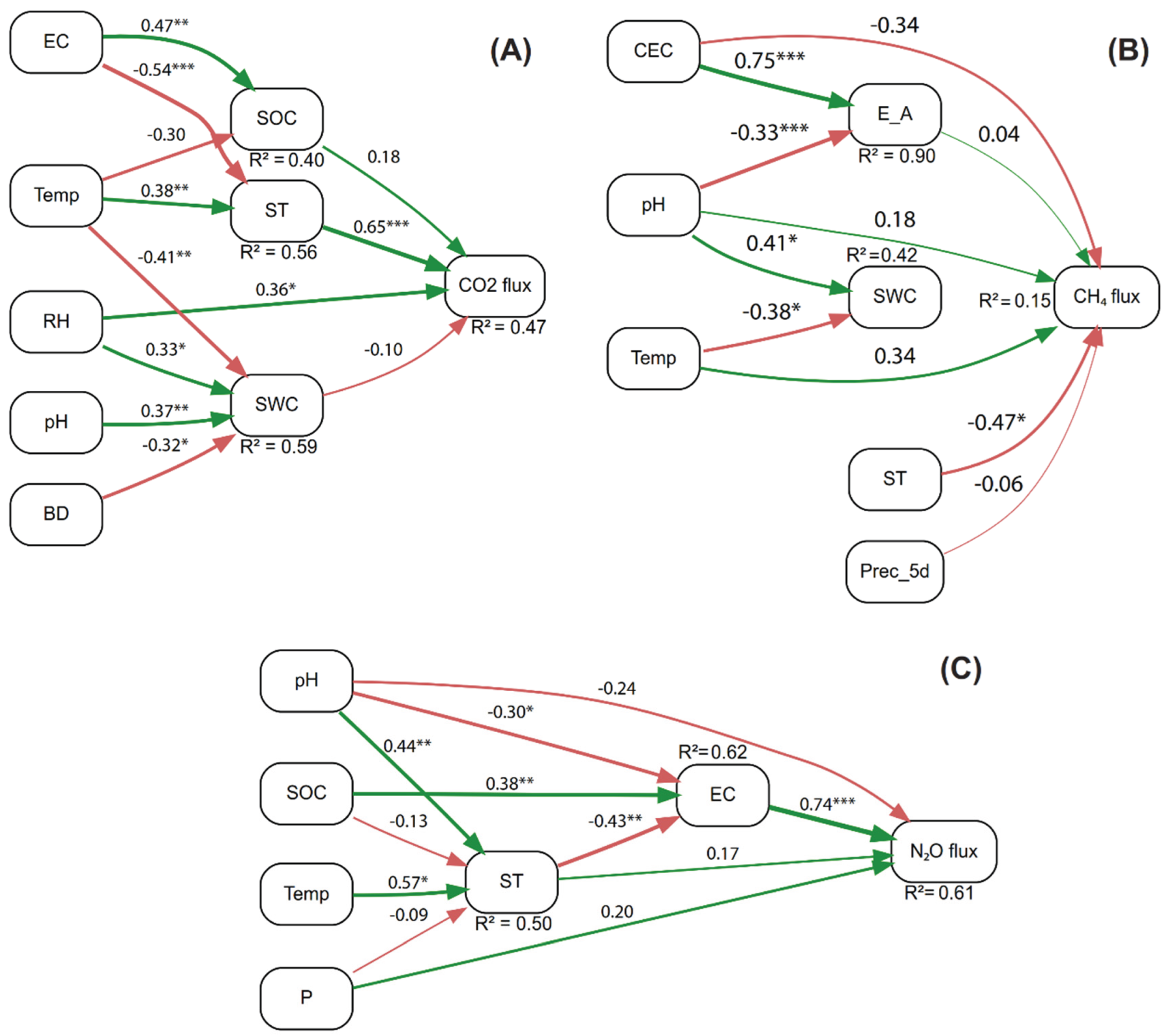
Table 2.
p-values from Spearman’s correlations between GHG fluxes (CO2, CH4, and N2O) and ST and SWC variables in different seasons.
Table 2.
p-values from Spearman’s correlations between GHG fluxes (CO2, CH4, and N2O) and ST and SWC variables in different seasons.
| Variable | Season | CO2 flux | CH4 flux | N2O flux |
| ST | Dry | 0.055 | 0.862 | 0.037 |
| ST | Rainy | 0.201 | 0.041 | 0.012 |
| SWC | Dry | 0.134 | 0.879 | 0.190 |
| SWC | Rainy | 0.288 | 0.057 | 0.894 |
Values in bold indicate statistically significant correlations at p < 0.05 (n= 35).
Table 3.
Global warming potential (GWP, in Mg CO2 eq ha-1 year-1) derived from total soil GHG (CO2, CH4, N2O) fluxes across seven land-use types in the Andean–Amazon transition zone, Caquetá, Colombia.
Table 3.
Global warming potential (GWP, in Mg CO2 eq ha-1 year-1) derived from total soil GHG (CO2, CH4, N2O) fluxes across seven land-use types in the Andean–Amazon transition zone, Caquetá, Colombia.
| Season | Land use | |||||||
| CaAS | CoAS | DP | IP | MPSE | OF | SFAE | ||
| GWP (Mg CO2 Eq ha-1 year-1) | Dry | 38.32 | 45.38 | 98.18 | 62.17 | 41.36 | 64.12 | 64.16 |
| Rainy | 34.44 | 36.54 | 70.29 | 57.15 | 38.29 | 56.66 | 57.71 | |
| Mean | 36.38 | 40.96 | 84.23 | 59.66 | 39.83 | 60.39 | 60.93 | |
GWP: Global warming potential. Values are presented for each season (dry and rainy) and as seasonal means. Land-use types include degraded pasture (DP), improved pasture (IP), cacao agroforestry system (CaAS), copoazu agroforestry system (CoAS), secondary forest with agroforestry enrichment (SFAE), moriche palm swamp ecosystem (MPSE), and old-growth forest (OF).
Disclaimer/Publisher’s Note: The statements, opinions and data contained in all publications are solely those of the individual author(s) and contributor(s) and not of MDPI and/or the editor(s). MDPI and/or the editor(s) disclaim responsibility for any injury to people or property resulting from any ideas, methods, instructions or products referred to in the content. |
© 2025 by the authors. Licensee MDPI, Basel, Switzerland. This article is an open access article distributed under the terms and conditions of the Creative Commons Attribution (CC BY) license (http://creativecommons.org/licenses/by/4.0/).
Copyright: This open access article is published under a Creative Commons CC BY 4.0 license, which permit the free download, distribution, and reuse, provided that the author and preprint are cited in any reuse.


