
Submitted:
25 December 2025
Posted:
26 December 2025
You are already at the latest version
Abstract
Cloud detection is an important procedure for the processing of remote sensing images. A cloud detection scheme driven by the spectral and the temporal features is presented in this paper, where an unsupervised hierarchy clustering approach is proposed for large scale image segmentation. The potential cloudy pixels are identified by means of the spectral matching, in which the spectral data of the clustering centers are compared to the patterns in the spectral dataset of ground covers. The matched pixels are regarded as cloudless pixels, whose category can be recognized accordingly. In contrast, the bright temperatures corresponding to the unmatched pixels are used to exclude the interference of the occasional hotspots, enabling the final cloud detection result. Landsat 8, Sentinel-2, and MODIS satellite data are used in the validation to demonstrate the precision and stability of the proposed scheme for the data at different spatial resolutions.
Keywords:
cloud detection
; unsupervised classification
; spectral feature
; temporal feature
1. Introduction
Cloud detection in remote sensing images is a critical component of remote sensing data preprocessing and analysis. Due to the strong scattering and reflection properties of clouds in optical bands, their presence significantly interferes with the acquisition of surface information, affecting the accuracy of feature extraction, classification, and subsequent quantitative analysis of ground objects. In the simulation of remote sensing images, cloud detection algorithms are typically first employed to determine the spatial distribution and coverage of clouds. Subsequently, radiative transfer and reflection models can be established for cloud-covered and cloud-free areas respectively to simulate the spectral response characteristics of different regions. By integrating the simulation results from both parts, remote sensing images with realistic cloud features can be generated. Therefore, cloud detection plays a vital role in remote sensing image simulation.
According to statistics, clouds cover approximately 66.7% of the Earth’s surface [1]. Among various remote sensing images of optical satellites, clouds appear as either the background for target detection or the disturbance for ground observation, which are expected to be identified before the implementation of other processing algorithms for data product generation [2,3,4].
Among various cloud detection method, the three types of features can be adopted to identify cloudy pixels in optical remote sensing images, i.e., the spectral, the temporal, and, the spatial features. Due to the fact that the reflectance of the clouds is much brighter than most of ground covers in the spectrum from visible to shortwave infrared (SWIR), while the emission of the clouds is generally weaker in medium and long wave infrared (MWIR and LWIR), a set of pixel-aligned images acquired in several to numbers of spectral bands with high transmittance, can be used to detect cloud by means of spectral classification [5]. The cloud detection method based on the temporal features generally assume that the spectral and the spatial features of the ground covers are steadily in a certain period. In this way, the cloudy pixels can be identified via anomaly pixel detection as long as the clear sky images of the same observational scene are available [6]. The spatial features of the clouds mainly refer to distribution, shape, and continuity, which represent as the textural characteristics in the remote sensing images. Thus, the cloudy pixels can be marked via image segmentation with the supplementary of either the spectral or the temporal information [7]. Besides, the mentioned features can be used in integrated manner to develop more accurate cloud detection method.
As a typical product of Earth meteorological activities, the features of the clouds are usually time-varying and probably transient. For this reason, the spectral reflectance of the clouds at a specific observational moment can hardly be predicted precisely to implement the spectral pattern identification for the cloudy pixels. In contrast, the spectral reflectance of the ground covers is predictable since the physical properties of the ground covers are invariant through a relative long period [8]. Thus, it is rational to achieve cloud detection using both the spectral and the temporal features. In detail, instead of modeling for cloud spectral reflectance, a spectral dataset of typical ground covers can be built to separate unknown pixels, which are probably cloudy. To improve detection accuracy, other events with instantaneous features should be considered, such as wildfire. As supplementary information, either MWIR or LWIR image can be adopted to identify clouds from wildfire according to the temperature difference.
With the mentioned idea, an efficient cloud detection scheme is presented for the processing of large-scale multispectral images in this paper, in which both the spectral and the temporal features of the clouds and the ground covers are considered. To this end, an unsupervised hierarchy clustering approach is proposed for large-scale image segmentation according to spectral reflectance difference. The spectral reflectance of the clustering centers is compared with the spectral patterns in ground cover dataset to identify the potential cloudy pixels. The radiant image acquired in the thermal infrared is used to eliminate the interference of the occasional hotspots for the final cloud detection result.
The remainder of the paper is organized as follows. The cloud detection scheme is detailed in Section 2, where the hierarchy clustering approach for large-scale image segmentation is proposed. The cloud detection results for Landsat 8, Sentinel-2, and MODIS data and the evaluation of the cloud detection algorithm are discussed in Section 3. Discussion of the results are presented in Section 4. And we conclude the paper in Section 5.
2. Proposed Approach
2.1. Dataset Overview
Common multi-spectral satellite systems primarily include the MODIS [9] and Landsat series [10] from the United States, the Sentinel series [11] led by the European Space Agency (ESA), and the Gaofen series (e.g., Gaofen-1, Gaofen-2, Gaofen-6) independently developed by China [12]. These satellite systems offer complementary capabilities in terms of spatial, temporal, and spectral resolutions, providing multi-scale and high-frequency data support for Earth observation research.
Multi-spectral remote sensing data products are typically categorized based on their processing levels, with common levels including Level-0 (L0), Level-1 (L1), and Level-2 (L2). L0 products consist of unprocessed raw data; L1 products refer to data that has undergone basic corrections such as radiometric calibration; L2 products represent data that has been further processed with systematic geometric correction based on L0 or L1 data. The specific classification methods are detailed in Table 1.
Landsat 8 and MODIS remote sensing data were selected to validate the cloud detection results. Their characteristics are introduced below.
2.1.1. Landsat 8
Landsat 8 is an Earth observation satellite launched by NASA on February 11, 2013. The satellite carries two primary sensors: the Operational Land Imager (OLI) and the Thermal Infrared Sensor (TIRS) [13]. Landsat 8 features 11 spectral bands: Bands 1–7 and 9 have a spatial resolution of 30 meters; Bands 10 and 11 have a resolution of 100 meters; and Band 8 (Panchromatic) has a resolution of 15 meters. Table 2 lists the band names, wavelength ranges, and spatial resolutions for Landsat 8.
Landsat 8 Level-2 (L2) data provides Surface Reflectance (SR) and Surface Temperature (ST) products. The raw values provided in the Level-2 data can be converted into surface reflectance and surface temperature using Equations (1) and (2):
Whereis the surface reflectance, is the surface temperature, and represents the raw digital number provided in the Level-2 data.
2.1.2. MODIS
The Moderate Resolution Imaging Spectroradiometer (MODIS) is carried onboard NASA’s Terra and Aqua satellites and is primarily used for global environmental change monitoring [14]. It is designed with high spatial resolution, extensive spectral bands, and high temporal resolution. Through further processing of raw remote sensing data, MODIS provides a series of data products. Specifically, the MOD06 product contains cloud detection results, the MOD09 product provides surface reflectance data, and the MOD11 product provides land surface temperature data. These products offer data support for researching cloud detection algorithms and the radiative scattering characteristics of clouds. Table 3 introduces selected bands relevant to surface reflectance and cloud detection.
2.1.3. Ground Object Spectral Reflectance Database
The latest version of the United States Geological Survey (USGS) Spectral Library is Version 7 [15]. This is a collection of spectral data acquired via laboratory, field, and airborne spectrometers. The database covers a wide wavelength range from ultraviolet to far-infrared, specifically from 0.2 to 200 μm. It includes spectral measurements of specific minerals, vegetation, chemical mixtures, and man-made materials. In many cases, samples were purified to ensure that the spectral properties of the materials are closely correlated with their chemical structures, forming effective spectral-chemical composition pairs, which is critical for interpreting remote sensing data. The library utilized the following four different spectrometers for measurements:
- Beckman 5270, covering 0.2–3 μm
- Analytical Spectral Devices (ASD), covering 0.35–2.5 μm
- Nicolet, covering 1.12–216 μm
- AVIRIS, covering 0.37–2.5 μm
These spectral data include not only natural mixtures of rocks, soils, and materials measured under laboratory conditions but also plant components and vegetation spectra under various background conditions, as well as forest vegetation spectra measured using airborne spectrometers.
2.2. Principal Method
Actual remote sensing imagery typically contains multiple spectral bands and covers extensive areas, resulting in massive data volumes where a single image often comprises a vast number of pixels. Adopting a pixel-by-pixel approach for cloud detection would lead to excessive computational resource consumption and low processing efficiency. Therefore, clustering is usually required as a preliminary step in the cloud detection workflow. The purpose of clustering is to group pixels with similar spectral features into the same category, thereby effectively reducing the computational complexity of subsequent processing [16]. By integrating pixels with similar spectral characteristics into unified analysis units through clustering, classification decisions can be made at the category level, significantly improving the computational efficiency of cloud detection.
The cloud detection scheme is presented in the Figure 1, where three major steps are involved, i.e., the hierarchy clustering, the identification of ground spectral pattern, and the exclusion of occasional interference. The scheme will be detailed in the following part of this section.
2.2.1. Hierarchy Clustering
For the versatility of the presented scheme, we assume that the prior information of the observational scene is unavailable. Thus, an unsupervised clustering approach is required to segment multispectral remote sensing image, which probably include millions of pixels. In this situation, the size of the difference or the similarity matrix for two arbitrary pixels is large enough to overflow the memory of an ordinary computer.
To improve the feasibility of the clustering procedure, a hierarchy clustering approach is proposed as shown in Figure 2, where the original three-dimensional multispectral data block with the size of N×M×L (i.e., NM pixels and L bands) is transformed into a two-dimensional matrix with the size of NM × L. Then, the pixels are randomly divided into number of groups, whose size is small enough for the calculation of the difference matrix in each group. The clustering centers from each group are assembled as the new two two-dimensional matrix, which can be divided again when its size is too large for the calculation of the difference matrix for two arbitrary clustering centers. The grouping and clustering procedure are repeated several times until the spectral data in the latest assembled clustering center matrix is small enough to generate its difference matrix for the final clustering result.
In each clustering step, the peak density search method [17] is adopted to determine the clustering centers. The local density of an arbitrary pixel is defined as
Where ρi is the local density of the pixel i; dij denotes the spectral difference between the pixel i to the pixel j; dc represents the difference threshold for the same class decision; and χ is the decision function, expressed as
The Euclidean distance is used to evaluate the difference and the similarity of two arbitrary spectrums, given as
where xik and xjk denote the corresponding spectral data of the pixel i and the pixel j, respectively.
When the local densities of all pixels are calculated using (3), they are sorted in a decreasing sequence according to the density. The first pixel in the sequence with the peak density is selected as the clustering center directly, whereas the belongings of the subsequent pixels are decided according to the minimal difference of the spectrum, which is defined as
where δi represent the minimal difference of the spectrum of the pixel i to the spectrums of the existing clustering center whose local density is higher than the pixel i. When the minimal difference δi is smaller than the difference threshold dc, the pixel is classified as the existing class with the update of local density. Otherwise, the pixel is selected as a new clustering center.
For the secondary and the subsequent clustering procedure, the clustering centers from the last stage are assembled and divided into a set of new groups. In each group, the local density is updated with
where ρiʹ denotes the local density of the clustering centers; and χʹ is the modified decision function, defined as
where ρj is the local density of the jth clustering center, which is calculated in the last stage of the grouping and clustering procedure.
As it can be seen, there are two criteria for clustering centers in the proposed approach. On one hand, the clustering centers are supposed to have a large local density, which characterizes the major component of the original image data. On the other hand, the spectrums of the clustering centers are expected to be significantly different from each other. For this reason, the candidates of the clustering center with either a small minimal difference or a low local density are excluded.
After the clustering centers of the specified image data are decided, the corresponding classified image can be generated by means of spectral matching.
2.2.2. Identification of Ground Spectral Pattern
The reflectance and the emission of the clouds are related to the physical properties, including height, water content, thickness, aspect angle, etc., which can vary rapidly in a relatively short period. For this reason, scarce spectral reflectivity data of the clouds are available to build spectral patterns of the clouds for detection. Instead, the cloudless pixels in the image corresponding to the ground area, can be detected via consulting the spectral dataset of the ground covers, in which the spectral reflectivity of most types of ground covers are involved. The remainder of the cloudless pixels are marked as clouds.
To this end, numbers of spectral reflectivity data are extracted from the U.S. Geological Survey (USGS) spectral library [18] to build a spectral dataset of the ground covers, including minerals, vegetation, chemical mixtures and man-made materials. The matching procedure is shown in Figure 3.
The spectral similarity of the clustering centers to the spectral patterns in the dataset of the ground covers can be quantify according to the Euclidean distance similar to (5), which can be expressed as
where Dij denote the similarity of the ith clustering center to the jth spectral pattern in the dataset; yik represent the reflectivity of the ith clustering center in the kth spectral band; and yjk represent the reflectivity of the jth spectral pattern in the kth spectral band.
Since the closer Euclidean distance corresponds to the higher similarity, the minimal distance of the ith clustering center to all spectral patterns in the dataset is selected as the criterion for the matching result, i.e.,
where si is the minimal distance of the ith clustering center to the spectral patterns; and Nʹ denotes the number of the spectral patterns in the dataset.
A threshold for the minimal distance can be set to decide whether the ith clustering center is matched, expressed as
where sc is the threshold for matching result decision; Mʹ denote total number of the cluster centers obtained in section II.A; C1 is an empirical constant describing the tolerance for unmatching, which is set as 2.6 in our experiment.
Note that due to the impacts of atmospheric effects, observational geometry and ground roughness, the spectral reflectivity of the same ground cover in the same image is different from one pixel to another. The additional tolerance can benefit the more accuracy matching results.
The decision function ξ for the spectral matching results is given as
For each matched clustering center, the type of the corresponding pixels can be identified, while the matched clustering centers indicate the possible cloudy pixels, which will be further examined to achieve the final detection result.
2.2.3. Exclusion of Occasional Interference
Since the cloud detection results depend on the completeness of the spectral dataset, occasional events corresponding to the unmatched pixels can be detected along with the clouds, including wildfire, air pollutant and rocket plume. Other available features should be adopted to alleviate the interference of the occasional events for the better performance of cloud detection.
In the field of satellite remote sensing, determining cloud temperature is a complex problem constrained by multiple factors. The results depend not only on macroscopic physical properties such as the optical thickness, cloud top height, and cloud phase, but may also be influenced by the internal microstructure of clouds and external atmospheric environmental conditions. Existing literature lacks studies that directly quantify the temperature range of clouds. The focus of this research is not to precisely define the temperature range of clouds but rather to utilize temperature information as an auxiliary discrimination feature to enhance the reliability of cloud detection.
The temperature of clouds is related to many physical properties, such as height, thickness, phase state, water and ice content, etc.
Although the dynamic temperature range of clouds is difficult to precisely define, cloud brightness temperature values are typically lower than those of the Earth’s surface and sporadic events such as wildfires and rocket plumes, and exhibit relatively lower temperature distribution characteristics across the entire remote sensing image. Based on this characteristic, by setting appropriate thresholds in the temperature imagery, cloud pixels can be effectively distinguished from sporadic event pixels, thereby further enhancing the accuracy and interference resistance of cloud detection.
The decision function ξʹ for exclusion of occasional interference is given as
where Tp denotes the bright temperature of the pth pixel in a specific LWIR spectral band; TM is the average bright temperature of the pixels corresponding to the ground cover, detected in Section II.B; and C2 is a weighting coefficient, which is set as a constant of 0.5 in our experiment.
The final detection result can be achieved after the exclusion of the pixels corresponding to the occasional events.
3. Results
3.1. Experimental Result
3.1.1. Clustering Result
Landsat 8, Sentinel-2 and MODIS data were selected to demonstrate the usefulness of the proposed scheme. The Landsat 8 data are detailed as an example, while only the cloud detection results of the other two types of satellite data are given. For one observational scene, Landsat 8 acquire the radiant images in eleven spectral bands, in which the bands NO. 1~7 are reflectance dominant bands with a spatial resolution of 30m. The band NO. 8 is the panchromatic band with a spatial resolution of 15m, while the band NO. 9 is the absorption band for cirrus detection. The bands NO. 10 and 11 locate at LWIR spectrum for temperature detection with a spatial resolution of 100m.
In this work, the images from the bands NO. 1~7 are used for the unsupervised hierarchy clustering, while the image from the band NO. 10 is adopted in the exclusion of the occasional interference. The pseudo-color and bright temperate images of the selected scene is shown in the Figure 4.
As it can be seen, the clouds covering a large are can be easily identified from either the pseudo-color image or the bright temperature image, whereas the fragmentary clouds covering a relatively small area can hardly be distinguished directly. The spectral features of the clouds are in accordance with our previous discussion, i.e., the cloudy pixels are brighter in the reflectance dominant spectral bands, while they are darker in the emission dominate spectral bands.
3.1.2. Cloud Detection Result
The hierarchy clustering result is given in the Figure 5, where the Figure 5(a) is the classification image, while the Figure 5(b) shows a part of the results for the spectral matching. As it can be seen in the Figure 5(a), there are 21 types of the objects in the classified image, while about 10 among them are probably clouds. The classification result validates our assumption that the spectral features of the clouds are transient and time-variant.
The spectral patterns of this work are extracted from the USGS spectral library [10]. The dataset includes 2455 spectral patterns in total, which covers spectrum from 0.35μm to 2.5μm at a resolution of 1nm. The Figure 5(b) shows an example of the spectral matching results, where the dots with different color denote the spectral reflectivity of the clustering centers extracted from the Landsat 8 data, while the curves with the corresponding color are the most similar pattern in the dataset.
As it can be seen in the Figure 5(b), when the dots of the same color distribute at the corresponding curve, the clustering center is perfectly matched. However, due to the interference of ground atmospheric effects, observational geometry and ground roughness, the dots generally distribute around the reference spectral pattern. These results demonstrate the necessity of an additional tolerance for the matching processing in (9).
The results of the method proposed in this paper are validated using Landsat 8, Sentinel-2, and MODIS data, and Figure 6 shows one set of results for each of these three satellite datasets. Columns (a), (b), (c), and (d) are respectively the RGB images, the cloud detection results of the proposed method, the reference cloud mask, and the difference between of the reference cloud mask to the cloud detection results of the proposed method. The detection image shows the similar texture to the reference image, whereas the boundary of the clouds in the two images are different, as shown in the Figure 6(d).
3.2. Experimental Evaluation
To quantitatively evaluate the accuracy of the cloud detection method, this chapter employs the confusion matrix method, as shown in Table 4, for analysis. Four metrics are selected to assess the accuracy and reliability of the results: Overall Accuracy (OA), Commission Error (CE), Omission Error (OE), and the Kappa coefficient.
Specifically, Overall Accuracy represents the proportion of correctly detected cloud pixels to the total number of pixels; Commission Error indicates the probability that a true non-cloud pixel is misclassified as a cloud pixel; Omission Error indicates the probability that a true cloud pixel is misclassified as a non-cloud pixel; and the Kappa coefficient is used to evaluate the agreement between the cloud detection results and the reference (ground truth) image. The formulas are as follows:
In the formulas, N is the total number of pixels, i.e., N = .
The evaluation metrics for the cloud detection results from the aforementioned Landsat 8 and MODIS imagery are presented in Table 5. The results show that after excluding interfering pixels, all metrics demonstrate improvement compared to the scenario where interfering pixels were not excluded.
In reference to the cloud mask product, the overall accuracy (OA), the commission error (CE), the omission error (OE) and the kappa coefficient of the final cloud detection result are analyzed [19], as shown in Table 6. Among the three types of remote sensing data, the OA of Sentinel-2 was 98.24% and the CE of 25.82%, which suggests that clear areas are more likely to be misclassified as clouds during cloud detection. For Landsat 8, the OA was 97.94% with the CE of 0.96%, demonstrating accurate cloud detection but with room for improvement in distinguishing clouds from other features. The OA of MODIS was 90.49% and the kappa value of 78.63%, indicating that the method is applicable in MODIS. The varying performance across the different remote sensing images could be attributed to the fact that higher spatial resolution images, such as those from Sentinel-2 and Landsat 8, contain more homogeneous spectral information per pixel, leading to less spectral mixing and, consequently, higher accuracy in matching with spectral databases.
In the cloud detection of Landsat 8 data, the FCNN method in [20] achieved an OA of 94.36%, with CE of 0.0536 and OE of 0.0591. The MSCFF method from [21] had an OA of 94.96%, CE of 0.0416, and OE of 0.0607. FMASK showed an OA of 89.59%, CE of 0.1338, and OE of 0.0699. While this method has a higher OA, its CE and OE are slightly higher than those of the other methods.
The Fmask algorithm, applicable to Landsat 4-9 and Sentinel-2 data, has become a widely recognized benchmark method for cloud detection. It was proposed by Zhu et al. [22] and has been iteratively updated. Fmask performs initial separation of cloud, cloud shadow, and snow/ice through multispectral threshold segmentation (e.g., utilizing shortwave infrared and cirrus bands) combined with morphological optimization. In this study, the Fmask method is adopted as a comparative benchmark to quantitatively validate the cloud detection performance of the proposed method on Landsat 8 imagery. The cloud detection results of the proposed method and the Fmask method on selected test samples are shown in Figure 7.
The evaluation metrics for the two methods applied to images from different scenes are presented in Table 7. The results indicate that the proposed method outperforms the Fmask method in terms of Overall Accuracy (OA), Commission Error (CE), and the Kappa coefficient, but is slightly weaker than the Fmask method regarding Omission Error (OE).
4. Discussion
The proposed cloud detection scheme, which integrates spectral and temporal features for large-scale multispectral image processing, demonstrates significant improvements in detecting clouds across various satellite platforms, including Landsat 8, Sentinel-2, and MODIS. Our results show that the method successfully identifies cloud and cloud-free pixels by matching spectral features from remote sensing imagery with a ground cover spectral dataset, coupled with a thermal infrared image to mitigate interference from occasional events like wildfires.
When comparing with previous studies, the cloud detection accuracy achieved in this work surpasses many conventional methods. For instance, the proposed method outperformed the widely recognized Fmask algorithm, especially in terms of overall accuracy (OA) and commission error (CE) when applied to Landsat 8 data. Specifically, the OA improved from 97.94% to 98.48% when excluding interference from sporadic events, highlighting the effectiveness of the additional temperature-based filtering step. However, the proposed method still exhibited slightly higher omission errors (OE) in complex cases, such as fragmented cloud boundaries or thin clouds, compared to Fmask.
This performance is consistent with existing studies that suggest spectral matching can successfully detect clouds by leveraging the inherent reflectance differences between clouds and ground covers. The accuracy of cloud detection was also influenced by spatial resolution, as higher resolution images (such as those from Landsat 8 and Sentinel-2) provided more homogeneous spectral information per pixel, improving the matching process and reducing spectral mixing.
While the method demonstrated strong results across different satellite data, challenges remain in distinguishing clouds from other transient events, such as smoke or pollutants, especially in regions with complex atmospheric conditions. Further research should explore advanced spectral models or machine learning techniques to better address these overlaps. Additionally, the dynamic nature of cloud reflectance and the potential for atmospheric interference suggest the need for more robust models that can account for these variations over time.
Future research could also focus on expanding the ground cover spectral database to include a broader range of environmental conditions, further enhancing the cloud detection accuracy. Moreover, integrating spatial features—such as texture and continuity—could provide additional context for cloud detection, which may improve detection in heterogeneous environments.
Overall, the results confirm that the proposed cloud detection scheme, with its emphasis on spectral and thermal infrared features, offers a promising solution for remote sensing applications, particularly when dealing with large datasets across varying spatial resolutions. As remote sensing technology continues to advance, future methods should aim to incorporate more dynamic, real-time cloud detection systems for enhanced environmental monitoring.
5. Conclusions
A cloud detection scheme using the spectral and the temporal feature difference of the cloud to the ground cover is presented in this paper. In case of the insufficient memory for the calculation of the pixel difference and the pixel similarity matrices, an unsupervised hierarchical clustering approach is proposed to classify the multispectral image with the typical spectral reflectivity for each class. The obtained spectral reflectivity data are compared to the spectral patterns in the spectral dataset of the ground cover. The unmatched pixels are marked as the potential cloudy pixels. A bright temperature image is adopted to exclude a part of the inference of the occasional events, including the wildfire and other hotspots, enabling the final cloud detection result.
Scenes from Landsat 8, Sentinel-2, and MODIS were selected to validate the proposed method. The classification images show the diversity of cloud spectral features. The detection results demonstrate the feasibility of cloud detection by matching spectral features from remote sensing satellite imagery with spectral databases. The method was tested on satellite data with different spatial resolutions. As shown in the results, the OA for Landsat 8, Sentinel-2, and MODIS is 97.94%, 98.24%, and 90.49%, respectively. The CE are 0.0096, 0.02582, and 0.0329, respectively. The OE are 0.1573, 0.0787, and 0.2324, respectively, while the corresponding Kappa values are 0.8990, 0.8127, and 0.7863.
A comparison was conducted between the proposed method and the Fmask method.The results indicate that for MODIS data, the overall accuracy of the detection outcomes exceeds 90%. Regarding Landsat 8 data, the proposed method outperforms the Fmask method in terms of overall accuracy, commission error, and the Kappa coefficient. However, it exhibits slightly weaker performance compared to Fmask in terms of omission error. Furthermore, the proposed method demonstrates a heightened propensity for omission errors (i.e., missed detection) when processing specific complex scenarios, such as cloud boundary regions, areas with fragmented small clouds, and zones covered by thin clouds.
The cloud detection scheme in this paper can also be used in hyperspectral data processing.
Author Contributions
Conceptualization, S.J.; methodology, W.S. and S.J.; software, S.J.; validation, W.S. and S.J.; formal analysis, W.S. and S.J.; investigation, S.J.; resources, W.S., S.J. and X.H.; data curation, W.S. and S.J.; writing—original draft preparation, W.S. and S.J.; writing—review and editing, W.S. and T.L.; visualization, T.L. and X.H.; supervision, X.H.; project administration, X.H.All authors have read and agreed to the published version of the manuscript.
Funding
This research received no external funding.
Data Availability Statement
The Landsat8 dataset are available at: https://www.gscloud.cn/; The Fmask data used for experimental evaluation are available at: https://github.com/GERSL/Fmask.
Acknowledgments
The authors gratefully acknowledge the providers of the datasets used in this study. We thank the data providers and the official platform for making these data publicly accessible.We also acknowledge the developers of the Fmask algorithm for providing an effective tool for cloud, cloud shadow, and snow detection in remote sensing imagery. The authors have reviewed and edited the output and take full responsibility for the content of this publication.
Conflicts of Interest
The authors declare no conflicts of interest.
References
- N. Ma, L. Sun, Y. He, C. Zhou, and C. Dong, “CNN-TransNet: A hybrid CNN-transformer network with differential feature enhancement for cloud detection,” IEEE Geosci. Remote Sens. Lett., vol. 20, pp. 1-5, 2023. [CrossRef]
- J. D. Braaten, W. B. Cohen, and Z. Yang, “Automated cloud and cloud shadow identification in landsat MSS imagery for temperate ecosystems,” Remote Sens. Environ., vol. 169, pp. 128–138, Nov. 2015. [CrossRef]
- P. Ebel, Y. Xu, M. Schmitt, and X. X. Zhu, “SEN12MS-CR-TS: A remote-sensing data set for multimodal multitemporal cloud removal,” IEEE Trans. Geosci. Remote Sens., vol. 60, 2022, Art. no. 5222414. [CrossRef]
- S. Sui and L. Sun, “Cloud Detection Fusion Algorithm for Complex and Variable Surface Conditions,” IEEE Geosci. Remote Sens. Lett., vol. 21, pp. 1-5, 2024, Art no. 5002305. [CrossRef]
- A. Fisher, “Cloud and cloud-shadow detection in SPOT5 HRG imagery with automated morphological feature extraction,” Remote Sens., vol. 6, no. 1, pp. 776–800, 2014. [CrossRef]
- C.-H. Lin, K.-H. Lai, Z.-B. Chen, and J.-Y. Chen, “Patch-based information reconstruction of cloud-contaminated multitemporal images,” IEEE Trans. Geosci. Remote Sens., vol. 52, no. 1, pp. 163–174, Jan. 2014. [CrossRef]
- Y. Chen et al., “An automatic cloud detection neural network for highresolution remote sensing imagery with cloud–snow coexistence,” IEEE Geosci. Remote Sens. Lett., vol. 19, 2021, Art. no. 6004205. [CrossRef]
- Z. Xiao, S. Liang, T. Wang, and Q. Liu, “Reconstruction of satelliteretrieved land-surface reflectance based on temporally-continuous vegetation indices,” Remote Sens., vol. 7, pp. 9844–9864, 2015. [CrossRef]
- Qin Y. W., Xiao X. M., Tang H., et al. Annual Maps of Forest Cover in the Brazilian Amazon from Analyses of PALSAR and MODIS Images[J]. Earth System Science Data, 2024, 16(1): 321-336.
- Choate M. J., Rengarajan R., Hasan M. N., et al. Operational Aspects of Landsat 8 and 9 Geometry[J]. Remote Sensing, 2024, 16(1): 133-167. [CrossRef]
- Pitkänen T. P., Balazs A., Tuominen S.. Automatized Sentinel-2 Mosaicking for Large Area Forest Mapping[J]. International Journal of Applied Earth Observation and Geoinformation, 2024, 127(10): 1-11. [CrossRef]
- Wang S T, Kang W, Kong D M, Wang T Z, et al. GF-1 Image Fusion Based on Regression Kriging[J]. Laser & Optoelectronics Progress, 2022, 59(8): 523-531.
- Zhu J H, Zhu S Y, Yu F C, et al. Downscaling of ERA5 Reanalysis Surface Temperature for Urban and Mountainous Areas[J]. Journal of Remote Sensing, 2021, 25(8): 1778-1791.
- Justice C. O., Townshend J. R. G., Vermote E. F., et al. An Overview of MODIS Land Data Processing and Product Status[J]. Remote Sensing of Environment, 2002, 83(1-2): 3-15. [CrossRef]
- Kokaly R. F., Clark R. N., Swayze G. A., et al. USGS Spectral Library Version 7: U.S. Geological Survey Data Series 1035. 2017.
- Xiang P. A Cloud Detection Algorithm for MODIS Images Combining K-means Clustering and Otsu Method[J]. IOP Conference Series: Materials Science and Engineering, 2018, 392(6).
- A. Rodriguez and A. Laio, “Clustering by fast search and find of density peaks,” Science, vol. 344, no. 6191, pp. 1492–1496, 2014. [CrossRef]
- R. F. Kokaly et al., “USGS Spectral Library Version 7: U.S. Geological Survey Data Series 1035,” Reston, VA, USA. [Online]. Available: https://crustal.usgs.gov/speclab/QueryAll07a.php.
- M. Hossin and M. N. Sulaiman, “A review on evaluation metrics for data classification evaluations,” Int. J. Data Mining Knowl. Manage. Process., vol. 5, no. 2, pp. 1–11, Mar. 2015. [CrossRef]
- D. López-Puigdollers, G. Mateo-García, and L. Gómez-Chova, “Bench-marking deep learning models for cloud detection in Landsat-8 and Sentinel-2 images,” Remote Sens., vol. 13, no. 5, p. 992, Mar. 2021.
- Z. Li, H. Shen, Q. Cheng, Y. Liu, S. You, and Z. He, “Deep learning based cloud detection for medium and high resolution remote sensing images of different sensors,” ISPRS J. Photogramm. Remote Sens., vol. 150, pp. 197–212, Apr. 2019. [CrossRef]
- Qiu S., Zhu Z., He B.. Fmask 4.0: Improved cloud and cloud shadow detection in Landsats 4–8 and Sentinel-2 imagery[J]. Remote Sensing of Environment, 2019, 231: 111205.
Figure 1.
Flowchart of cloud detection scheme.
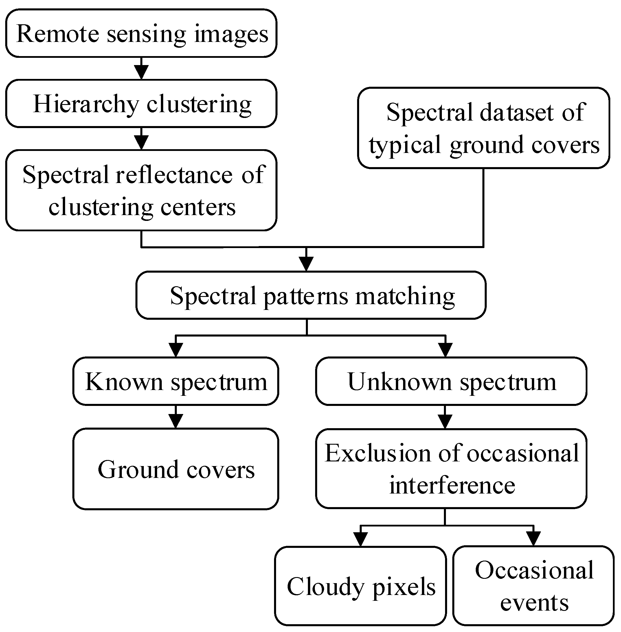
Figure 2.
Schematic diagram for hierarchy clustering of spectral images.
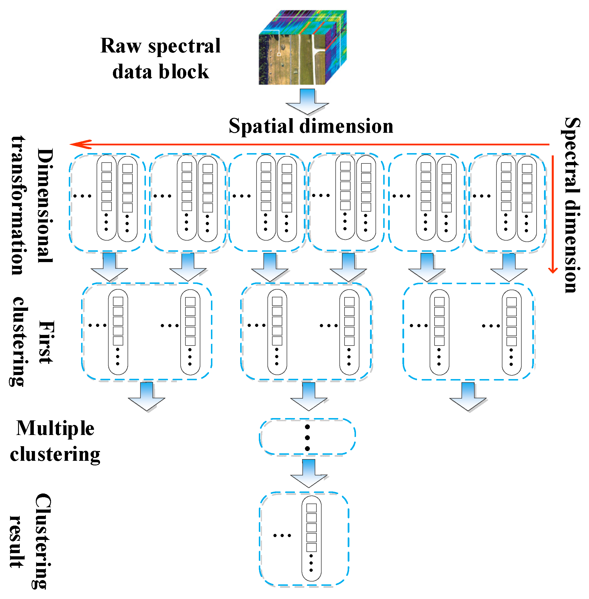
Figure 3.
The process of computing vector D for a certain type of data.
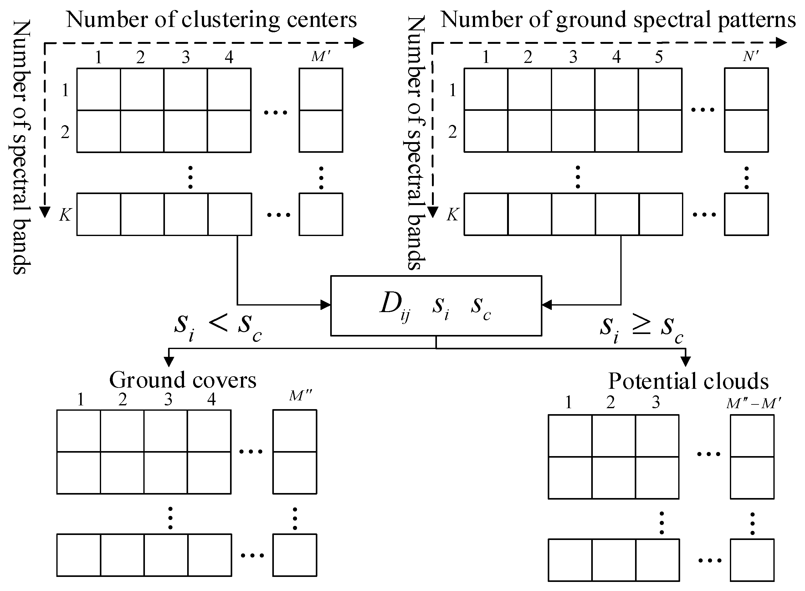
Figure 4.
Selected test scene of Landsat 8 data. (a) Pseudo-color image synthesized with red, green, and blue bands. (b) Bright temperature image of band NO. 10, where brighter dots indicate higher temperatures and the black pixels in the middle indicate that information is missing and unavailable.
Figure 4.
Selected test scene of Landsat 8 data. (a) Pseudo-color image synthesized with red, green, and blue bands. (b) Bright temperature image of band NO. 10, where brighter dots indicate higher temperatures and the black pixels in the middle indicate that information is missing and unavailable.
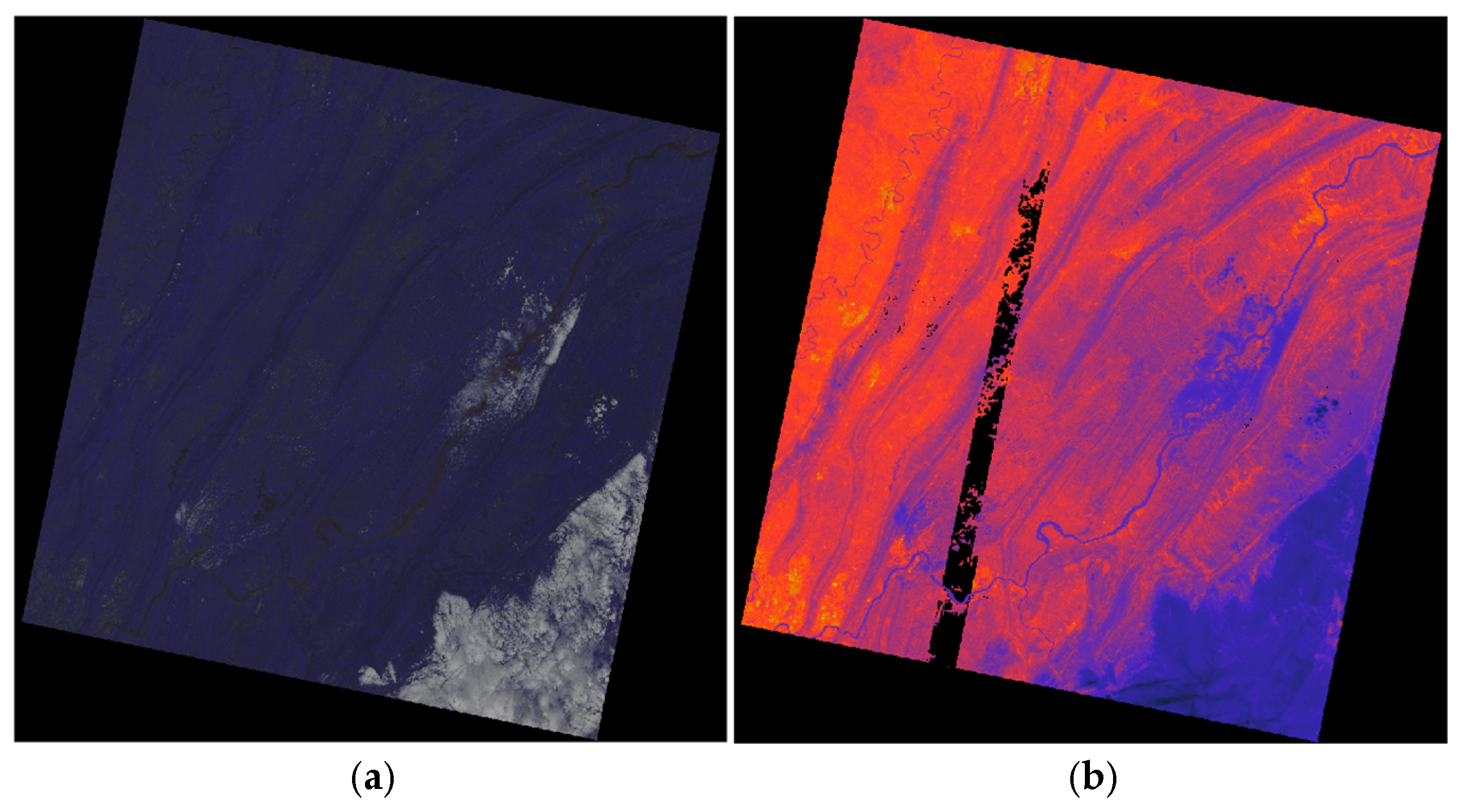
Figure 5.
(a) Classification image. (b) Spectral reflectivity of clustering centers and their most similar patterns in dataset. Dots represent spectral reflectivity of clustering center, while solid lines are spectral patterns in dataset.
Figure 5.
(a) Classification image. (b) Spectral reflectivity of clustering centers and their most similar patterns in dataset. Dots represent spectral reflectivity of clustering center, while solid lines are spectral patterns in dataset.
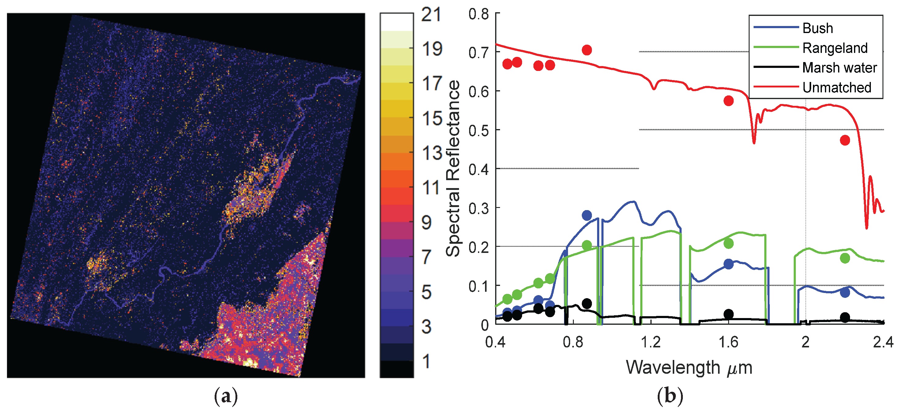
Figure 6.
Cloud detection results. The first row displays the results for Landsat 8, the second row for Sentinel-2, and the third row for MODIS. (a) RGB imagery. (b) Cloud detection results using the proposed method, where white and cyan represent cloud and clear sky, respectively. (c) Reference cloud mask. (d) Difference between (b) and (c), where red, yellow, and cyan denote false alarm pixels, false omission pixels, and correct detection results, respectively.
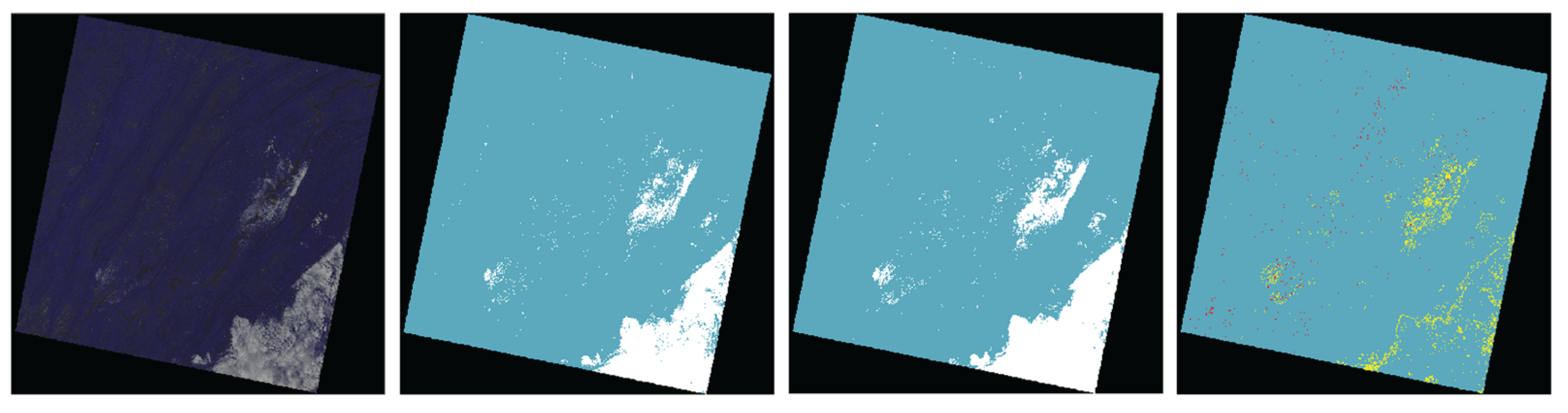
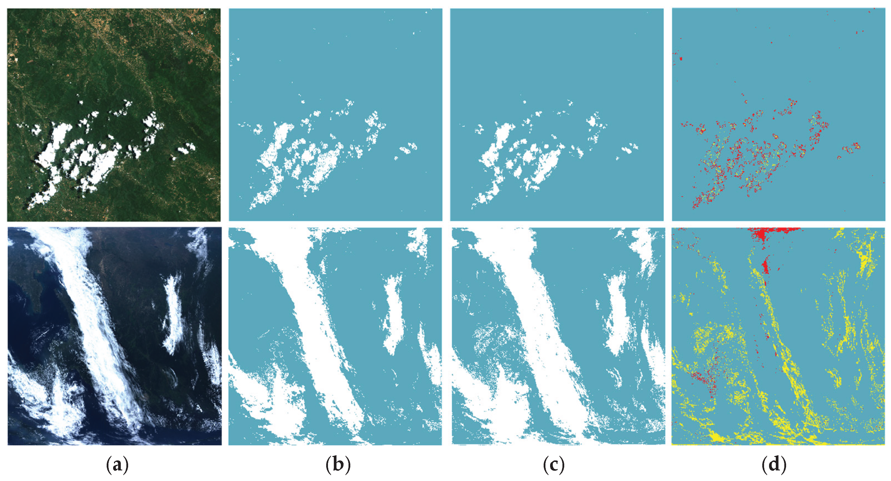
Figure 7.
Evaluation of the Proposed Method and the Fmask Method.
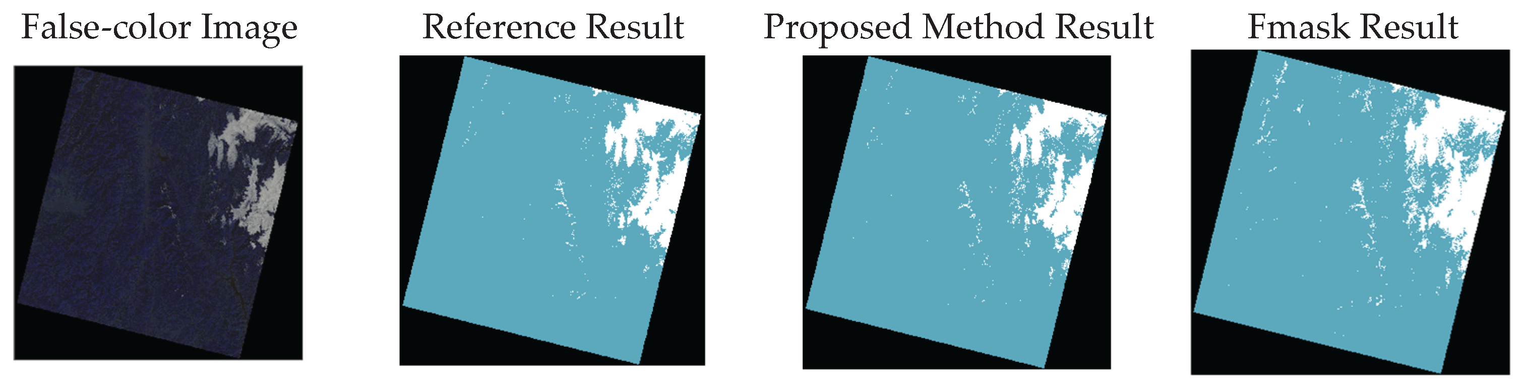
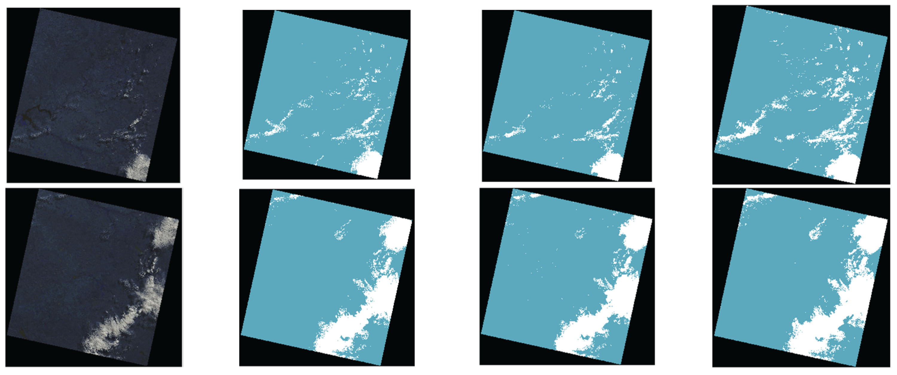

Table 1.
Classification of Satellite Spectral Data.
| Classification | Level | Designation | Description |
|---|---|---|---|
| Data Products | L0 | Raw Data Image | Data directly acquired by remote sensingsatellite sensors. Raw data without any processing. |
| L1 | System Radiometric Correction Product | Image products that have undergone system radiometric correction and spectral restoration but have not undergone geometric correction. | |
| L2 | System Geometric Correction Product | Data products based on L1 data that have undergone systematic geometric correction or have been projected onto a specific map coordinate system. |
Table 2.
Introduction to Landsat 8 Bands.
| Landsat 8 | |||
|---|---|---|---|
| Band Name | Wavelength Range(μm) | Spatial Resolution (m) | |
| Operational Land Imager (OLI) | Band 1 Coastal | 0.43-0.45 | 30 |
| Band 2 Blue | 0.45-0.51 | 30 | |
| Band 3 Green | 0.53-0.59 | 30 | |
| Band 4 Red | 0.64-0.67 | 30 | |
| Band 5 NIR | 0.85-0.88 | 30 | |
| Band 6 SWIR1 | 1.57-1.65 | 30 | |
| Band 7 SWIR2 | 2.11-2.29 | 30 | |
| Band 8 Pan | 0.50-0.68 | 15 | |
| Band 9 Cirrus | 1.36-1.38 | 30 | |
| Thermal Infrared Sensor (TIRS) | Band 10 TIRS1 | 10.6-11.19 | 100 |
| Band 11 TIRS2 | 11.5-12.51 | 100 | |
Table 3.
Introduction to Selected MODIS Bands.
| Channel | Spectral Range (μm) | SNR | Primary Use | Resolution (m) |
|---|---|---|---|---|
| 1 | 0.62-0.67 | 128 | Land, Cloud Boundaries | 250 |
| 2 | 0.841-0.876 | 201 | 250 | |
| 9 | 0.438-0.448 | 838 | Ocean Color, Phytoplankton, Biogeochemistry | 1000 |
| 10 | 0.483-0.493 | 802 | 1000 | |
| 12 | 0.546-0.556 | 750 | 1000 | |
| 13 | 0.662-0.672 | 910 | 1000 | |
| 16 | 0.862-0.877 | 516 | 1000 | |
| 26 | 1.36-1.39 | 150 | Cirrus Clouds | 1000 |
| 32 | 11.77-12.27 | 0.05 | Surface & Cloud Top Temperature | 1000 |
| 33 | 13.185-14.085 | 0.25 | 1000 |
Table 4.
Confusion Matrix for Accuracy Validation of Cloud Detection Results.
| Type | Cloud Detection Results from Remote Sensing Image | ||
| Cloud | Non-Cloud | ||
| Cloud Detection Results | Cloud | γ11 | γ12 |
| Non-Cloud | γ21 | γ22 | |
Table 5.
Evaluation of Cloud Detection Results.
| OA | CE | OE | Kappa | |
|---|---|---|---|---|
| Landsat 8 (without excluding interference) |
0.9806 | 0.0338 | 0.1252 | 0.9037 |
| Landsat 8 (excluding interference) |
0.9848 | 0.0132 | 0.1096 | 0.9275 |
| MODIS | 0.9049 | 0.0329 | 0.2324 | 0.7863 |
Table 6.
Evaluation of Cloud Detection Results.
| OA | CE | OE | Kappa | |
|---|---|---|---|---|
| Landsat 8 | 0.9794 | 0.0096 | 0.1573 | 0.8990 |
| Sentinel-2 | 0.9824 | 0.2582 | 0.0787 | 0.8127 |
| MODIS | 0.9049 | 0.0329 | 0.2324 | 0.7863 |
Table 7.
Comparison Between the Proposed Method and Fmask.
| Scene 1 | Scene 2 | Scene 3 | Average | |||||
| Proposed | Fmask | Proposed | Fmask | Proposed | Fmask | Proposed | Fmask | |
| OA | 0.9829 | 0.9695 | 0.9817 | 0.9602 | 0.9805 | 0.9622 | 0.9817 | 0.9640 |
| CE | 0.0563 | 0.2359 | 0.1022 | 0.3859 | 0.0556 | 0.1788 | 0.0723 | 0.2669 |
| OE | 0.1213 | 0.0022 | 0.1980 | 0.0023 | 0.0556 | 0.0005 | 0.1248 | 0.0017 |
| Kappa | 0.9006 | 0.8485 | 0.8375 | 0.7399 | 0.9321 | 0.8785 | 0.8899 | 0.8223 |
Disclaimer/Publisher’s Note: The statements, opinions and data contained in all publications are solely those of the individual author(s) and contributor(s) and not of MDPI and/or the editor(s). MDPI and/or the editor(s) disclaim responsibility for any injury to people or property resulting from any ideas, methods, instructions or products referred to in the content. |
© 2025 by the authors. Licensee MDPI, Basel, Switzerland. This article is an open access article distributed under the terms and conditions of the Creative Commons Attribution (CC BY) license (http://creativecommons.org/licenses/by/4.0/).
Copyright: This open access article is published under a Creative Commons CC BY 4.0 license, which permit the free download, distribution, and reuse, provided that the author and preprint are cited in any reuse.


