
Submitted:
22 December 2025
Posted:
23 December 2025
You are already at the latest version
Abstract
Understanding when and where to shift land from agriculture to forestry is essential for developing sustainable land-use strategies that balance climate, biodiversity, and rural development goals. Traditional profitability comparisons rely on long-term discounting, which is sensitive to assumptions and misaligned with the decision-making horizons of landowners and policymakers. This study introduces a deposit-based framework that treats annual timber biomass growth as accumulating economic value, enabling direct comparison with yearly agricultural profits on a per-hectare basis. By integrating parcel-level spatial data, land quality indicators, national statistics, and expert input, the framework generates high-resolution maps of annual profitability for both land uses. Applied in Latvia, the analysis reveals significant regional variation in agricultural returns, with many low-quality areas showing marginal or negative profits, while forestry offers stable, modest gains across diverse biophysical conditions. The results highlight where afforestation becomes a financially rational alternative and suggest transition pathways that enhance overall land-use profitability while supporting climate and biodiversity objectives. The framework is transferable to other contexts by substituting context-specific data on land quality, prices and growth, and can complement policy instruments such as performance-based CAP payments and afforestation support. The approach supports future-oriented differentiated land-use planning using annually updated spatial economic signals.
Keywords:
afforestation
; land use profitability
; parcel-level assessment
; sustainable land management
; land quality
; crop groups
; regional differentiation
1. Introduction
Land is a limited resource that must serve multiple, often competing demands, including food production, timber supply, biodiversity conservation, and climate change mitigation. In recent decades, global population growth and rising incomes have increased demand for food, particularly animal-based products [1]. This trend has contributed to the large-scale conversion of forests into agricultural land [2,3], while urban expansion has further intensified pressure on natural land resources [4]. Even well-intentioned policies to reduce agricultural intensity can lead to unintended environmental impacts, such as indirect land use change and deforestation elsewhere [5].
In response, afforestation is gaining political momentum as a key element of climate and biodiversity strategies. The European Union (EU) has committed to ambitious afforestation targets in support of its climate neutrality and biodiversity restoration goals [6,7,8]. Countries such as Ireland and Spain have introduced national afforestation plans to expand forest cover, increase carbon sequestration, and improve ecosystem services [9,10]. Similar initiatives are also underway in Brazil and India [11,12].
Despite these efforts, afforestation policies are often met with hesitation from landowners, particularly in the agricultural sector. Concerns include the risk of higher land prices and food insecurity [19], potential restrictions on converting land back to farming [6], the long time periods before financial returns are received, and changes in soil properties that may reduce agricultural productivity [14,15,16].
Nevertheless, some researchers, such as Rämö et al. (2023), argue that transforming not only unused but also low-yield agricultural land into forests is essential for meeting ambitious climate targets [17]. Similarly, West et al. (2020) found that afforesting low-productivity grasslands can also be financially beneficial [18]. These findings support the broader view that land with limited agricultural potential, due to poor soil quality, low fertility, or other biophysical constraints, offers greater opportunity for land use change without significantly affecting food production.
At the same time, several experts suggest that innovations in agriculture, particularly precision farming, may help optimise land use efficiency [19,20,21]. By ensuring that high-yield crops are cultivated on the most suitable land, marginal or less productive areas could be freed up for afforestation [22]. Financial incentives and support for sustainable farming practices, combined with education and awareness programmes, can further encourage farmers to adopt such integrated approaches [23,24].
Financial considerations are central to land use decisions, especially where land is treated as an economic asset. Landowners generally seek to maximise returns, making the relative profitability of agriculture and forestry a key factor in decisions about land use change [25]. Yet, comparing the two systems is methodologically difficult. Agriculture typically generates annual profits, whereas forestry provides returns only a few times over a rotation cycle that may span several decades. Discounting methods are commonly used to make these comparisons [26,27,28], but they depend heavily on long-term assumptions about future prices, costs, and interest rates. Even small changes in these assumptions can significantly affect the outcome, potentially reversing the conclusion from afforestation being more profitable than agriculture to the opposite.
In this study, we present a parcel-level framework for comparing the annual profitability of agricultural and forestry land uses. This approach is designed to reduce reliance on long-term discounting methods, which can be difficult to interpret and highly sensitive to assumptions. Instead, we treat the annual growth of timber biomass as an accumulating economic value, enabling a more transparent and consistent comparison with agricultural profits. The framework integrates spatial data, land quality assessments, official statistics, and expert knowledge to calculate land profitability at a high resolution. We apply the method to a case study from Latvia, where afforestation is increasingly relevant in light of climate policy targets and structural challenges in agriculture. This framework supports regionally differentiated land use strategies by identifying where afforestation presents a financially viable alternative to agriculture. By enabling transparent, spatially explicit assessments of profitability, it contributes to the design of adaptive and multi-objective land management policies that align with economic viability, climate mitigation, biodiversity conservation, and rural development.
2. Materials and Methods
2.1. Case Region
The case region for this study is Latvia, a Northern European country located in the temperate cool moist climate zone. Approximately 50% of Latvia`s territory is forested, while about one-third is designated as agricultural land. Latvia is sparsely populated, with a population density of 30 persons per square kilometre as a country average, and 10 persons per square kilometre for rural areas [29].
Agricultural land in Latvia is almost entirely privately owned and managed by individual farmers or enterprises. As of the end of 2023, Latvia had 62 thousand agricultural holdings, with large holdings managing half of the total agricultural land. In contrast, 46% of forest land is owned and managed by the state, while the remaining 54% is under the ownership of private individuals, municipalities, or other entities.
The agricultural sector in Latvia is primarily oriented towards cereal and milk production, positioning the country as a net exporter of these commodities. In total, the agricultural area covers approximately 1.97 millions hectares, of which 1.36 millions hectares is arable land. The average land area per agricultural holding is 45 hectares, with 31 hectares being agricultural land. Despite strong performance in certain sectors, domestic production of vegetables, fruits, and berries remains insufficient to meet national consumption needs. In 2023, the total agricultural output at current prices amounted to 1.85 billion euros [29]. As a member of the European Union, Latvia operates under the Common Agricultural Policy (CAP), benefiting from financial support mechanisms similar to those available in other EU member states.
In Latvia, forests are a significant national resource, both economically and ecologically. Forest stands are predominantly composed of pine (25.6%), birch (27.2%), and spruce (19.6%), together accounting for 72.4% of the total forest area. Other notable species include grey alder (10.1%), aspen (8.2%), black alder (6.3%), ash and oak (1.0%), and a variety of other species (2.1%). In 2022, a total of 13.1 million cubic meters of wood were harvested in Latvia, with 6.4 million cubic meters sourced from state forests and 6.7 million cubic meters from forests owned by private entities. Forest restoration efforts covered an area of 41 thousand hectares [30].
2.2. Methodology Description
The methodology is structured as a comprehensive framework for calculating and comparing the annual profitability of agricultural and forest land uses at the parcel level. All calculations are conducted on a per-hectare basis to ensure consistency and comparability across land-use types and regions. The analysis integrates spatial data with economic and biophysical indicators relevant to each sector.
For agriculture, average annual profitability (XA) is calculated for different crop groups and livestock specialisations using farm accountancy data, complemented by expert evaluations and calibrated against official statistics.
For forestry, a deposit-based approach is applied: potential profit (XF) associated with the average annual accumulation of timber biomass in forests eligible for harvesting is treated as a financial deposit. This value is calculated based on the net income potential of standing volume growth, incorporating current prices and species-specific yield assumptions. Total timber accumulation, accumulation of harvestable timber and financial parameters are calibrated against official statistics.
The methodology begins with the development of equations required to calculate annual profitability for both agricultural and forest land uses. These equations incorporate key variables such as yields, prices, production costs, and land characteristics. Once the equations are established, relevant input data are collected and processed, including spatial land parcel data, statistical records, and species-specific growth parameters. Parameter values are derived from national statistics, official registers, published research, and expert assessments. A schematic representation of the full methodology is provided in Figure 1, and each methodological component is explained in detail in the following subsections.
Detailed descriptive statistics on the Latvian agricultural and forestry sectors, as well as extended tables of parameter values, are provided in the Appendices. The main text reports only the information necessary to apply and interpret the framework, while all supporting details remain available for replication and adaptation in other regions.
2.2.1. Profitability in Agriculture
In this study, agricultural land profitability is defined as the net profit before taxes per hectare of land or per grazing animal. Profitability is calculated for the major crop groups (cereals; rapeseeds; pulses; potatoes; vegetables, strawberries, flowers; perennial crops; other crops (e.g. nectar plants, herbs, flaxseed, lavender, chamomile, caraway); fallow land; grassland in arable land; meadows and pastures) and major grazing animal groups (dairy cows; suckler cows; sheep). The poultry and pig sectors are excluded from the analysis as these animals are typically not directly linked to nearby land use.
To calculate agricultural profitability (XA), data from the Latvian Farm Accountancy Data Network (FADN) [31], Latvian Rural Advisory and Training Centre (LLKC) Gross Margin data [32], and expert evaluations are used. Anonymised FADN data at the individual farm level was used. The calculations are based on data from 2019, 2020, and 2021. The years 2022, 2023, and 2024 are excluded from the analysis due to atypically high profitability in major agricultural sub-sectors. Farms are classified into four groups based on the size of the managed area, as summarised in Annex A1, taking into account differences in productivity, costs, and revenues associated with farm size.
Prices (PA) for agricultural products were obtained from national statistics on the purchase prices of agricultural products for the period 2019 to 2021 [33]. Yields are calculated for each crop and farm size group from national statistics, with annual yields varying by crop type and farm size group [32,34]. In certain cases, yields are also influenced by land quality and the farming system employed (conventional or organic). Calculated profitability parameters per farm size and farming system are detailed in Annex A2.
In this study, land quality is indexed from 5 to 85 points, with a weighted average of 36 points. Although the methodology for land quality indexing was developed over 40 years ago, it is based on a detailed and comprehensive evaluation framework that remains relevant for comparative analysis today. The index was originally designed to estimate the potential rye yield in kilograms per hectare, with one land quality point corresponding to 70 kilograms of rye per hectare [35]. Particular emphasis in the assessment methodology was given to soil related characteristics, including soil type, granulometric composition, and agrochemical properties. These were considered alongside a broader set of biophysical and site-specific variables, such as natural environmental conditions, moisture regime, drainage infrastructure, topography, parcel size and configuration, stoniness, microdepression occurrence, and the degree of land cultivation. Historical parcel level land quality data, based on this methodology, cover a significant portion of agricultural land in Latvia [36], enabling spatially detailed assessments despite the historical origin of index. For parcels lacking historical data, land quality is estimated using the average of the nearest neighbouring parcels. While the index corresponds with rye yields, its linear structure allows it to remain useful for other crops as well, when combined with appropriate correction coefficients. These coefficients are calculated by dividing the average annual productivity of crop groups (cereals, rapeseeds, and pulses) from statistical data by the average land quality points and are refined or adjusted as necessary [37]. It is important to note that land quality is not a determining factor in all agricultural sectors. In this study, it is considered only in cases where its influence is clearly observable, most notably in crop production.
Almost every market-oriented farmer in Latvia submits spatial information about all fields and crops used for production to the Rural Support Service in order to apply for support payments. Using this data (prepared by the Rural Support Service upon request) and overlaying it with the land quality index data layer, it is possible to calculate the indicative profitability of each field using the formula in Figure 1.
Additionally, all animal holdings are registered with the Agricultural Data Center, which provides information on the number of animals. By using this data along with the location coordinates of the holdings (prepared by the Agricultural Data Center upon request), it is possible to calculate the indicative profitability of each grazing animal holding.
Although the FADN dataset offers detailed information for approximately one thousand individual farms, there are notable limitations that complicate the accurate assessment of profitability indicators. A key issue is that many farm operators do not allocate themselves a formal wage. Instead, the value of their labour is covered by the remaining profit after expenses, which is often done to reduce taxable income. This practice can lead to an overstatement of reported profits, particularly on smaller farms with minimal or no hired labour. As a result, land use profitability may appear higher than it actually is, since the cost of the farmer's own labour is not included. Additionally, the majority of farms in the dataset use mixed production systems, involving several outputs such as different crops or types of livestock. However, cost data are usually reported for the entire farm as a whole, without breaking them down by specific activity. This lack of detail makes it difficult to assess how profitable each type of production really is.
To address the first challenge, labour costs are adjusted by recalculating them using labour salary data from national statistics [38], rather than relying solely on bookkeeping records. This recalculation involves multiplying the sum of paid and unpaid labour inputs [39] by the agricultural labour salary. Since larger and technologically advanced farms typically employ more qualified labour, salary rates are adjusted based on farm size. In many instances, particularly for smaller farms, this recalculation of labour costs results in increased expenses and consequently reduces the profits indicated in the FADN data.
To address the second challenge, calculations are performed by selecting individual FADN farms with potentially narrow specialisations. However, notable differences in results between farms often persist. Therefore, corrections are made using LLKC Gross margin calculations. These calculations provide standard incomes and costs for different crop groups (cereals, rapeseeds, and pulses, potatoes, vegetables, strawberries, flowers, perennial crops, other crops, fallow land, grasslands in arable land, meadows and pastures), animals (dairy cows, suckler cows, sheep), farming systems (conventional and organic), and farm sizes (large, medium, small, micro).
The category of other costs encompasses various farm expenses that are essential for agricultural production and farm maintenance, such as fertilisers and plant protection products, animal feed, fuel, machinery and equipment maintenance, and services and equipment rental. One significant component of this category is depreciation, which increases with the capital intensity of a farm. Higher capital investment in machinery, equipment, and infrastructure leads to greater depreciation expenses. This trend reflects the economic burden associated with maintaining and replacing capital assets over time [31].
The results of our calculations are cross-validated against statistical data from the Eurostat [40]. This ensures that our aggregated parcel-level estimates are consistent with national statistics.
2.2.2. Profitability in Forestry
Unlike agriculture, profit in forestry is typically generated only 2 to 3 times during a stand rotation cycle, which ranges from 30 to 100 years depending on the dominant tree species. This results in a situation where yearly profits in forestry are largely negative or close to zero, but significantly high during felling years. Consequently, direct comparisons of forestry profitability with agricultural production, which generates profit annually, are challenging.
To calculate forestry investment profitability, discounting methods are commonly used [41]. However, this approach relies on long-term assumptions about prices, inflation, and interest rates. Even minor changes, for instance, in interest rate assumptions over a 70-year period can substantially impact discounted values, making projection results highly sensitive to long-term assumptions. This results in a wide range of scenarios with significant differences between minimum and maximum outcomes [42]. Moreover, if forestry profitability results are to be compared with agricultural profitability, agricultural profits must also be calculated and discounted over the same long-term period, facing similar challenges of assumptions over an extended timeframe.
To address these challenges, in this study, forestry is instead conceptualised as an economic deposit, where annual increments in standing timber volume are treated as additions to a latent profit balance that materialises when the land or standing stock is sold. This perspective reframes forestry as generating an implicit yearly income stream, comparable in temporal resolution to agricultural profits, while avoiding long-term discounting of uncertain future flows.
For each forest stand, the annual deposited profit XF (EUR per hectare per year) is defined as the product of species- and site-specific net income per hectare of forest stand (EUR per hectare per year) and the annual increment in standing volume Zv (m3 per hectare per year). Net income per hectare of forest stand is obtained as the difference between expected revenues from assortments (EUR per m3) and the full set of logging and regeneration costs at current prices. The cumulative deposit (EUR per hectare) at time is then the sum of annual deposited profits since stand establishment, representing the unrealised yet quantifiable economic value stored in the standing stock.
Due to the structure of the available data, we have initially calculated the cumulative deposit (EUR per hectare) of each dominant tree species and forest type at the end of the rotation cycle. Then, by dividing the cumulative deposit into years corresponding to the length of the rotation cycle of each dominant tree species, we have calculated the annual deposited profit (EUR per hectare per year). The length of the rotation cycle for different dominant species is determined in Section 9 of the Law on Forests of the Republic of Latvia [43].
The expected revenues from assortments have been calculated based on the assumption that the proportion of assortments depends on the dominant species and the forest type [44]. The proportion of assortments is multiplied by the price for the respective assortment and the felling stock at the end of rotation cycle, obtaining revenues of final felling (EUR per ha). Revenues of thinning have been calculated by multiplying the proportion of assortments with the price for respective assortments and the thinning stock. The price of assortments depends on the dominant tree species, and the assortment type [45]. The thinning stock has been calculated by multiplying the annual increment in standing volume with the times and age of thinning (3 times at age 30, 46 and 60 for conifers and 2 times at age 20 and 40 for deciduous trees, for grey alder and aspen – 1 thinning at age 20) and the coefficient 0.3 (assuming that 30% of the total stock is removed with thinning (for spruce the coefficient is 0.2)) [46]. Data for assortment proportion and prices used in the calculations can be found in the Annex A3.
The regeneration costs consist of the forestry measures after the final felling: soil preparation, purchase of planting material, planting, forest protection, agrotechnical maintenance, felling for maintenance of the composition and underbrush tending. The costs associated with soil preparation, planting material, planting, agro-technical practices, and young forest stand maintenance are derived from statistical data on forest regeneration and maintenance expenses for 2024 [47]. The costs of young stand protection include labour compensation for this activity, set at 100 euro in 2024 [48], and 36 euro for repellents [49]. Supplementation costs consist of seedling and planting expenses, adjusted by coefficients of 0.3 (assuming that, on average, 30% of the stand requires supplementation) and 0.5 (assuming that labour costs are by 50% lower). Underwood clearing costs are estimated based on industry practitioners’ evaluations [50]. The annual maintenance cost of land amelioration systems is estimated at EUR 23 per hectare, based on expert assessment. It is assumed that these systems require maintenance every five years. Accordingly, the total maintenance cost over a given rotation cycle is calculated as EUR 23 multiplied by the ratio of the rotation cycle (in years) to five. This provides a simplified estimate of cumulative maintenance expenditure per hectare over the rotation cycle. The regeneration costs used in this study can be found in Annex A4.
The logging costs of rotation cycle consist of the expenses arising from the preparation and transportation of the assortments in thinning and final felling. The logging costs per unit of harvested wood (EUR per m3) are derived from statistical data on average expenses of forest exploitation for 2024 [51]. The costs of thinning (EUR per hectare) have been calculated by multiplying the costs of thinning per unit of harvested wood (EUR per m3) with the thinning stock per hectare (m3 per hectare) for each dominant tree species. The costs of logging (EUR per hectare) have been calculated by multiplying the costs of logging per unit of harvested wood (EUR per m3) with the total felling stock (m3 per hectare) at the end of rotation cycle for each dominant tree species. Logging costs are attached in the Annex A5.
Calculations for the annual increment in stand volume per hectare are based on equations that incorporate data about the main dominant species, site index, stand basal area, and age of the stand. Parcel level data for the dominant species, site index, stand basal area, and age of the stand are from State Register of Forests [52]. The coefficients used in the calculation of the stand growth are specified in Annex A6. Furthermore, to avoid extreme values, the calculated stand growth is aligned with the maximum standing volume per hectare from Donis (2019) which depends on the dominant species and the site index [53] (Annex A7).
To ensure the accuracy and reliability of our findings, our calculations are validated against statistical data from the Eurostat [40]. Similarly to agriculture, this ensures that our aggregated parcel-level estimates align with statistical aggregates.
2.3. Mapping at Parcel Level
In this study, profitability calculations were conducted at the individual field level to account for the specific characteristics and management practices of each parcel. However, for spatial visualisation and data privacy purposes, the field-level results were aggregated into a uniform grid with cells of 100 hectares each. By standardising the data into regular 100-hectare grid cells, we enabled a more consistent and comparable spatial representation of profitability across the case region, while preserving high spatial resolution. This method aligns with established practices in spatial land use analysis, where various aggregation techniques, such as the use of regular square grids, are used to harmonise heterogeneous data and support cross-regional comparisons [54]. Additionally, grid-based aggregation simplifies complex field geometries, improving the clarity and usability of spatial data for analysis and interpretation.
2.4. Technical Implementation
Profitability modelling and spatial data processing were performed in R version 4.4.1. Initial data preparation and spatial operations were implemented in R through the RStudio interface, using dplyr for data processing and sf for the management and transformation of spatial objects. The tidyverse and janitor packages were employed to streamline data manipulation, cleaning, and the standardisation of tabular datasets, ensuring consistent and analysis-ready inputs. Map creation, visualisation, and exploratory spatial analysis were carried out using the tmap, tmaptools, and leaflet packages, which enabled the production of both static and interactive cartographic outputs suitable for detailed spatial interpretation.
During the preparation of this work the author used ChatGPT-4 by OpenAI in order to enhance the phrasing of certain sentences and to correct potential grammatical errors, as none of the authors are native English speakers. After using this tool, the authors reviewed and edited the content as needed and take full responsibility for the content of the publication.
3. Results
3.1. Per-Hectare Profitability Patterns for Agricultural and Forest Land
Profitability in agricultural land use varies considerably across different crop groups and land quality points. As shown in Figure 2, profitability is strongly influenced by land quality: land with a quality score above 45 is classified as high-quality agricultural land. In such areas, local municipalities often impose restrictions on land use changes to preserve the productive potential of land.
Cereals and pulses show consistently positive profitability across all land quality classes, reflecting their relatively low input requirements and stable market demand. In contrast, the profitability of vegetables, potatoes, and perennial plantations tends to decline sharply on lower quality land. In many cases, particularly in marginal areas, these crops show negative returns, despite having positive average profitability values overall. These crop groups are more input and labour intensive, making them less economically viable on soils of lower quality.
Meadows and pastures generally show lower profitability compared to cultivated crops. This reflects their primary function in supporting the livestock sector through feed provision, sustainable grazing, and ecosystem services, rather than generating direct market revenue. As illustrated in Figure 2, the profitability of meadows and pastures is several times lower than that of cereals, rapeseeds, and pulses. However, when these grasslands are used as feed sources within livestock sector, they contribute significantly to overall farm profitability.
Other crop groups may yield high returns depending on the interaction between crop-specific characteristics and land quality. Notably, high profitability tends to occur where favourable yield and price conditions align with relatively low input requirements and depreciation costs.
While land quality is a key determinant of agricultural profitability, farm size is also a critical factor influencing economic outcomes. As the Figure 3 show, larger farms tend to achieve higher profitability, benefiting from economies of scale, more efficient use of inputs, and better access to modern technologies and markets. In contrast, smaller farms, particularly micro farms, often face structural disadvantages that limit profitability. This is especially evident in capital- and labour-intensive sectors such as vegetable, potato, and perennial plantations production. For instance, micro farms operating in perennial plantations show average losses exceeding 2 500 EUR/ha. These losses would be even more pronounced without income support, highlighting the structural dependence of small and micro farms on subsidy payments to maintain continued production.
Grassland systems used for dairy production also show negative profitability for smaller farms, while meadows and pastures used for suckler cow systems tend to be modestly profitable. Cereals, rapeseeds, and pulses maintain stable positive returns across all farm sizes, likely due to lower input intensity and higher compatibility with mechanised farming. The other crops category also shows high profitability, particularly for larger farms, possibly reflecting specialisation in high value or niche production, such as like mustard, flaxseed, nectar plants, and herbs (e.g. lavender, chamomile, and caraway).
Yearly profitability in forest land use ranges from 4 to 266 EUR per hectare, depending on the dominant tree species and forest growth conditions. While revenue primarily depends on the main tree species, costs vary based on forest growth conditions. Coniferous species, such as pine and spruce, are highly profitable across all forest growth conditions due to their high assortment prices and the larger proportion of high value assortments, particularly saw logs.
Although birch saw logs are not produced in Latvia, a significant share of birch is sold as veneer logs, which represent the most valuable tree assortment. This makes birch one of the most profitable tree species. In contrast, the profitability of deciduous species such as black alder, grey alder, and aspen is lower, as these trees mainly yield packing case timber, pulpwood, and firewood, lower-quality assortments that fetch lower prices.
Other tree species, including oak, ash, and linden, exhibit the highest profitability due to their superior assortment quality, high market prices, and relative rarity in Latvia. When comparing profitability across different forest growth conditions, the highest returns are achieved on dry mineral soils, while the lowest are observed on wet organic soils. This is because, despite higher forestry costs, dry soils tend to produce significantly higher yields per hectare (Figure 4).
3.2. Mapping Agricultural and Forest Land Profitability
Figure 5 illustrates substantial spatial variation in agricultural profitability across Latvia. The highest profitability levels (in dark blue) are concentrated in limited areas, primarily in the southern part of the country. However, these high-profit zones are relatively sparse. The majority of agricultural land falls within the moderate profitability range (in medium blue), with widespread distribution across central, western, and parts of eastern Latvia. Areas with low profitability (in light blue) or financial losses (in red) are more prevalent in the eastern, southeastern, and some north-central regions.
This spatial distribution reflects the influence of both natural and structural factors. Soils with lower fertility, smaller and fragmented land parcels, and limited market access contribute to the lower profitability observed in certain regions. In contrast, areas with better soil conditions, more consolidated farms, and improved infrastructure tend to perform better economically.
In contrast, forestry profitability (Figure 6) shows a more spatially consistent distribution, with the majority of grid cells falling within the low to moderate profitability range (in light and medium blue). High-profit areas (in dark blue) are relatively limited and scattered, while zones with negative returns (in red) are rare and highly localised. This overall pattern indicates that forestry offers relatively stable, though modest, economic returns across a wide range of biophysical conditions. As such, forestry may represent a more resilient land use option in areas where agricultural profitability is low or highly variable.
4. Discussion
4.1. Profitability Trade-Offs Between Agriculture And Forestry
The profitability analysis across agricultural and forest land use systems reveals that not all agricultural activities are economically viable, particularly on small and micro farms cultivating vegetables and potatoes, perennial crops or managing grasslands. In cases where agricultural land consistently operates at a loss, there is a growing rationale to consider alternative land-use production systems. One such option is afforestation, which, in certain conditions, offers not only competitive profitability but also additional ecosystem benefits. Targeted afforestation, particularly with species like spruce or birch, which have shown strong profitability on dry and drained mineral soils, and drained organic soils, may serve as a productive alternative, especially when aligned with climate, biodiversity, and rural development goals. This perspective does not advocate afforestation across all low-performing farmland, but it does support strategic integration of forestry into land use planning, where economic performance, soil characteristics, and farm structure indicate limited agricultural viability.
This aligns with findings by Lubowski, Plantinga, and Stavins (2006), who showed that land quality is a key determinant of the opportunity cost of afforestation and the potential supply of carbon sequestration from land use change [55]. Their analysis demonstrated that higher quality agricultural land is less likely to be converted to forest, as its productivity in crop production increases the economic trade-offs of afforestation. These findings highlight the importance of incorporating regional land use characteristics and local economic conditions into assessments of afforestation potential and policy design.
Returning to methodological challenges, Rämö et al. (2023) demonstrate that higher interest rates necessitate increased subsidies to make forestry as profitable as agriculture [17]. West et al. (2020) determined the net present value of forests over a 30-year rotation cycle by considering the anticipated felling volumes, prices, and management costs for various assortments [18]. They then converted the net present value into equivalent annual payments using a discount rate of 8%. Consequently, discounting leads to a lower net present value of forestry at higher interest rates. In contrast, the forest profitability methodology we propose accounts for the specific year of calculation, price fluctuations, and biomass growth. This approach enables relatively precise annual calculations of the required support payments to achieve income equivalence with agriculture.
The deposit-based measure differs conceptually from standard net present value (NVP) in three ways: 1) it uses current prices and costs without projecting future trajectories; 2) it expresses forestry returns as an annual flow comparable to agricultural profit; and 3) it captures the option value of selling land or standing timber before the end of a full rotation [56]. In practice, this means that the ranking of land-use options may diverge from NPV-based assessments, especially under high interest rates or volatile price expectations.
4.2. Institutional Constraints and Policy Implications
Both agriculture and forestry provide benefits that extend beyond individual owners and managers, offering societal value by ensuring food production, raw materials, water and nutrient cycling, climate change mitigation, and the preservation of the rural environment. Our proposed approach can be complemented with evaluations of these additional benefits.
The previous Rural Development Program (2014-2020) of Latvia included support for the forest industry in restoring, preserving, and improving forest ecosystems. The measures were actively used for improving drainage systems in forests, afforestation, enhancing ecological value, and protecting Natura 2000 forest areas, thereby reducing costs, and generating additional income for owners [57]. However, these support measures are insufficient to motivate a significant number of landowners to afforest their land. Many small and micro farmers, as indicated by Nipers and Pilvere (2020), are often seniors and lack spare financial resources [58]. They rely on current cash flows and lack economic mobility, making it challenging for them to find the financial resources needed to invest in afforestation, even with the available support measures. Additionally, West et al. (2020) indicate that incentives for ecosystem services payments are restricted to the first forest rotation, and enrolment in afforestation programmes on various factors other than profitability [18].
While this study focuses primarily on profitability, which is a significant factor for landowners who view their land as a financial asset, it is important to acknowledge other factors, which may influence land use change decisions. Environmental benefits, such as carbon sequestration, biodiversity conservation, and water purification, which align with the aims of the EU Green Deal to achieve climate neutrality, the Paris Agreement's goal to limit global warming to well below 2 degrees Celsius, the EU Biodiversity Strategy's objective to protect and restore ecosystems, and the EU Water Framework Directive's aim to achieve good qualitative and quantitative status of all water bodies, play a crucial role in the broader assessment of land use options.
Switching from agricultural production to forestry will impact net GHG emissions reduction. For instance, in Lithuania, maintaining a stable land use change pattern, where small areas are deforested but large areas are afforested, reaching 32 thousand hectares annually, alongside increased conversion from cropland to grassland, could ensure compliance with the EU target for 2030 [59]. Thus, afforestation could have a beneficial impact at the national or regional level, helping to achieve climate ambitions. Additionally, converting part of agricultural land to forest can partially offset agricultural emissions, thereby reducing the farm's GHG footprint. However, it is crucial to recognise that afforestation alone will not suffice to achieve climate targets.
Afforestation of agricultural land can also significantly affect biodiversity and water quality. By transforming open agricultural fields into forested areas, habitat diversity increases, supporting a broader range of species and enhancing biodiversity [60,61]. However, this may not apply in forest-rich countries. Regarding water quality, afforestation can reduce soil erosion and surface runoff, common in agricultural landscapes [62]. Tree roots stabilise the soil, reducing sediment and agricultural chemicals entering water bodies, thereby improving water quality by decreasing levels of pollutants such as nitrates, phosphates, and pesticides [63].
Additionally, social impacts, such as rural development and community well-being, should be considered to provide a comprehensive assessment of land use options [64]. Transitioning from agricultural production to forestry affects social dynamics due to differing labour input intensities between these sectors [65,66]. Widespread afforestation may influence job opportunities, particularly in rural areas, potentially reducing employment in agriculture while creating new roles in forestry.
By integrating the aforementioned factors into the proposed methodology, policymakers can make more informed decisions that balance economic, environmental, and social objectives. This is particularly important in considering afforestation as a key strategy for achieving carbon neutrality by 2050. Consequently, it is essential to recognise that preserving all agricultural land at any cost is not always justifiable. Financially unsustainable production practices that fail to generate sufficient profit and rely heavily on social support mechanisms do not foster the continuation of farming by future generations and should therefore be reconsidered.
Over the past two to three decades, the structure of agriculture in the EU has changed significantly. Between 2005 and 2020, the number of farms in the EU declined by approximately 37%, representing a reduction of 5.3 million farms, of which around 87% were small farms under 5 hectares [67]. This structural shift raises important questions for policymakers regarding the justification of continued support for such farms, particularly as maintaining this segment of the agricultural sector requires substantial financial resources, primarily through the CAP. Allocating funds to financially unsustainable farms may reduce the availability of resources for other political objectives. From a long-term perspective, it is more appropriate to direct support towards farms that can continue operating while contributing to the sustainability goals of the EU Green Deal. To ensure the effective and efficient use of public funds, support should be linked to measurable outcomes.
Evidence from China’s nature reserves, as shown by Cheng, Sims, and Yi (2023), demonstrates that conservation policies prioritising measurable environmental outcomes can deliver clear ecological benefits [68]. However, the study also highlights that the distribution of economic gains may be uneven and influenced by local development conditions. To ensure the effective and efficient use of public resources, support distribution should be based on measurable outcomes, such as environmental performance indicators. Within this context, the CAP plays a critical role by offering subsidies and incentives for sustainable land management practices that aim to balance ecological responsibility with economic viability [69]. By promoting a collaborative, results-oriented approach involving all relevant stakeholders, it is possible to advance ambitious climate goals while maintaining food security and protecting the livelihoods of farmers [70].
4.3. Transferability and Generalisation of the Framework
This study applies the land-use profitability framework to Latvia, but the underlying logic is designed to be transferable to other regions and policy contexts. The framework has three core components: 1) a consistent methodology for calculation annual agricultural profit and forestry deposit flows at the parcel level; 2) integration of spatial, biophysical and economic data to derive these indicators; and 3) spatial mapping of profitability patterns to support informed evaluation of where afforestation could be considered as a viable economic alternative to agriculture. Only the empirical parameterisation of these components is country-specific, while the structure of the approach is generalisable.
Transferring the framework to new contexts mainly requires the replacement of input data with region-specific information on land quality, farming systems, and economic conditions. Land quality indices, for example, can be replaced with national measures such as soil classification, climatic zones, or productivity indices used in national land evaluation systems [71]. Agricultural profitability can be estimated using data from farm accountancy networks, surveys, or standard gross-margin budgets where harmonised farm-level data (e.g. FADN) are not available [72]. Forestry parameters can likewise be adjusted to reflect region-specific species composition, assortment structures, and market prices.
Because the framework relies on transparent, annually based indicators, it can be easily recalibrated using updated or region-specific input data. Changes in prices, costs, or support levels can be readily incorporated, enabling the framework to remain relevant under evolving economic conditions and data availability. This adaptability supports its integration into existing data systems and allows for consistent comparison across different regions or time periods.
4.4. Multi-Objective Land-Use Planning And Future Research Directions
While this study primarily focuses on economic profitability, the proposed framework holds considerable potential for advancing multi-objective land-use planning. By enabling parcel-level comparisons of agricultural returns and forestry deposit values, it establishes a strong foundation for integrated assessments that align economic, environmental, and social policy goals. When combined with spatial indicators such as labour demand, net GHG emissions, or habitat quality, the framework can support the strategic identification of land-use transitions that deliver co-benefits for climate mitigation, biodiversity conservation, and rural development.
This direction aligns with growing recognition in land-system science that land-use decisions must account for overlapping and sometimes competing objectives [73,74,75]. Parcel-level profitability maps can serve as a critical layer in spatial planning tools, guiding where afforestation, extensification, or landscape restoration could deliver both ecological and economic gains. Such tools are increasingly necessary to operationalise national climate strategies, biodiversity targets, and the EU Green Deal commitments in spatially explicit and cost-effective ways.
Importantly, the framework also provides a basis for addressing social equity and territorial cohesion. In many marginal areas, continued agricultural activity is sustained through undercompensated labour or dependence on subsidies [76], raising concerns about the long-term viability and fairness. Identifying where these patterns persist can inform just transition policies that combine environmental objectives with measures to support rural livelihoods, sustain services, and mitigate social risks.
Looking forward, further research should focus on expanding the framework to incorporate additional performance indicators beyond profitability. Existing spatial methodologies for evaluating employment outcomes [39] and biodiversity [77] demonstrate the feasibility of a multi-criteria assessment approach. Developing an integrated decision-support system that includes these dimensions would allow policymakers to better assess trade-offs and synergies across multiple objectives, including climate resilience, food security, ecosystem integrity, and social well-being.
Finally, the framework establishes a basis for more adaptive and evidence-based land-use policy in the future. Its structure is well-suited for integration into tools that can incorporate regularly updated data, allowing policymakers to respond to changing economic and environmental conditions as they emerge. This capacity for gradual refinement is particularly important in regions where land-use dynamics are influenced by both global pressures and local constraints. In this way, the proposed approach offers a scalable and transferable foundation for supporting sustainable land-use transitions
5. Conclusions
This study highlights the importance of incorporating spatially explicit profitability assessments into land use planning and policy development. Profitability varies significantly across land quality, farm size, crop types, and dominant tree species showing that uniform land management strategies are insufficient. Integrating profitability data into decision making can help identify areas were afforestation, agricultural support, or diversification efforts would be most effective. This study contributes a scalable and transferable approach to land-use assessment that goes beyond profitability. It lays the groundwork for an integrated, evidence-based land management system, capable of informing targeted, just, and climate-smart policies across diverse territorial contexts. As future research expands its multi-objective capabilities, the framework can serve as a central tool in the transition toward sustainable and resilient land-use systems.
Author Contributions
Conceptualization, K.B. and A.N.; methodology, K.B., U.D.V., A.N.; software, U.D.V., K.B.; validation, K.B. and A.N.; formal analysis, U.D.V., K.B.; investigation, A.N.; resources, A.N., I.P..; data curation, K.B., U.D.V., A.N.; writing—original draft preparation, K.B., U.D.V.; writing—review and editing, A.N., I.P.; visualization, U.D.V., K.B.; supervision, A.N.; I.P.; project administration, I.P.; funding acquisition, I.P. All authors have read and agreed to the published version of the manuscript.
Funding
The research was promoted with the support of the project Strengthening Institutional Capacity for Excellence in Studies and Research at LBTU (ANM1), project No. 5.2.1.1.i.0/2/24/I/CFLA/002, sub-project No. 3.2.-10/187 (AF14).
Data Availability Statement
The data presented in this study are openly available in DataverseLV at: https://doi.org/10.71782/DATA/KINURI.
Conflicts of Interest
The authors declare no conflicts of interest.
Appendix A1

Table 1.
Farm size groups in different agricultural sectors
| Agricultural sector | Farm size, ha | |||
| Large farms | Medium farms | Small farms | Micro farms | |
| Cereals, rapeseeds, pulses | >300 | >100, ≤300 | >20, ≤100 | ≤20 |
| Vegetables (with potatoes) | >30 | >10, ≤30 | >2, ≤10 | ≤2 |
| Perennial plantations | >30 | >10, ≤30 | >2, ≤10 | ≤2 |
| Other crops (e.g. mustard, flaxseed, nectar plants, herbs, lavender, chamomile, caraway) | >150 | >50, ≤150 | >10, ≤50 | ≤10 |
| Fallow land | >300 | >100, ≤300 | >20, ≤100 | ≤20 |
| Grasslands | >300 | >100, ≤300 | >20, ≤100 | ≤20 |
| Meadows and pastures | >300 | >100, ≤300 | >20, ≤100 | ≤20 |
| Dairy cows (with calves) | >200 | >30, ≤200 | >4, ≤30 | ≤4 |
| Suckling cows (with calves) | >200 | >30, ≤200 | >4, ≤30 | ≤4 |
Appendix A2
Table 1.
Estimated data for cereal production equations
| Factor | Large farms | Medium farms | Small farms | Micro farms |
| Conventional farms | ||||
| Price (EUR/t) | 196.84 | 196.84 | 177.16 | 157.47 |
| Average yield (t/ha) | land quality points * 0.1076574 | |||
| Support (EUR/ha) | 149.85 | 149.85 | 149.85 | 149.85 |
| Labor costs (EUR/ha) | 140.25 | 154.00 | 197.12 | 291.06 |
| Other costs and depreciation (EUR/ha) | 512.59 | 497.21 | 451.08 | 435.70 |
| Organic farms | ||||
| Price (EUR/t) | 272.07 | 272.07 | 244.87 | 217.66 |
| Average yield (t/ha) | land quality points * 0.1280373 | |||
| Support (EUR/ha) | 266.85 | 266.85 | 266.85 | 266.85 |
| Labor costs (EUR/ha) | 140.25 | 154.00 | 197.12 | 291.06 |
| Other costs and depreciation (EUR/ha) | 486.96 | 472.35 | 428.52 | 413.91 |
Table 2.
Estimated data for rapeseeds production equations
| Factor | Large farms | Medium farms | Small farms | Micro farms |
| Conventional farms | ||||
| Price (EUR/t) | 477.62 | 477.62 | 429.86 | 382.10 |
| Average yield (t/ha) | land quality points * 0.0426049 | |||
| Support (EUR/ha) | 187.85 | 187.85 | 187.85 | 187.85 |
| Labor costs (EUR/ha) | 140.25 | 154.00 | 197.12 | 291.06 |
| Other costs and depreciation (EUR/ha) | 627.10 | 608.29 | 551.85 | 533.03 |
| Organic farms | ||||
| Price (EUR/t) | 744.06 | 744.06 | 669.65 | 595.25 |
| Average yield (t/ha) | land quality points * 0.0525616 | |||
| Support (EUR/ha) | 266.85 | 266.85 | 266.85 | 266.85 |
| Labor costs (EUR/ha) | 140.25 | 154.00 | 197.12 | 291.06 |
| Other costs and depreciation (EUR/ha) | 595.74 | 577.87 | 524.26 | 506.38 |
Table 3.
Estimated data for pulses equations
| Factor | Large farms | Medium farms | Small farms | Micro farms |
| Conventional farms | ||||
| Price (EUR/t) | 251.81 | 251.81 | 226.63 | 201.45 |
| Average yield (t/ha) | land quality points * 0.0706193 | |||
| Support (EUR/ha) | 221.94 | 221.94 | 221.94 | 221.94 |
| Labor costs (EUR/ha) | 140.25 | 154.00 | 197.12 | 291.06 |
| Other costs and depreciation (EUR/ha) | 503.86 | 488.74 | 443.40 | 428.28 |
| Organic farms | ||||
| Price (EUR/t) | 413.44 | 413.44 | 372.10 | 330.75 |
| Average yield (t/ha) | land quality points * 0.0784871 | |||
| Support (EUR/ha) | 318.94 | 318.94 | 318.94 | 318.94 |
| Labor costs (EUR/ha) | 140.25 | 154.00 | 197.12 | 291.06 |
| Other costs and depreciation (EUR/ha) | 478.67 | 464.31 | 421.23 | 406.87 |
Table 4.
Estimated data for vegetable and potato production equations
| Factor | Large farms | Medium farms | Small farms | Micro farms |
| Conventional farms | ||||
| Price (EUR/t) | 273.07 | 273.07 | 273.07 | 273.07 |
| Average yield (t/ha) | 22.41 | 21.06 | 17.32 | 12.84 |
| Support (EUR/ha) | 376.78 | 376.78 | 376.78 | 376.78 |
| Labor costs (EUR/ha) | 2 010.25 | 3 118.50 | 3 665.20 | 3 081.54 |
| Other costs and depreciation (EUR/ha) | 2 200.43 | 2 134.41 | 1 936.38 | 1 870.36 |
| Organic farms | ||||
| Price (EUR/t) | 427.65 | 427.65 | 427.65 | 427.65 |
| Average yield (t/ha) | 9.30 | 7.86 | 7.18 | 5.68 |
| Support (EUR/ha) | 939.90 | 939.90 | 939.90 | 939.90 |
| Labor costs (EUR/ha) | 2 010.25 | 3 118.50 | 3 665.20 | 3 081.54 |
| Other costs and depreciation (EUR/ha) | 2 090.41 | 2 027.69 | 1 839.56 | 1 776.84 |
Table 5.
Estimated data for production of perennial plantations equations
| Factor | Large farms | Medium farms | Small farms | Micro farms |
| Price (EUR/t) | 1 737.43 | 1 737.43 | 1 737.43 | 1 737.43 |
| Average yield (t/ha) | 7.30 | 6.86 | 5.64 | 4.18 |
| Support (EUR/ha) | 285.64 | 285.64 | 285.64 | 285.64 |
| Labor costs (EUR/ha) | 2 187.90 | 3 395.70 | 3 985.52 | 3 354.12 |
| Other costs and depreciation (EUR/ha) | 7 978.81 | 7 739.45 | 7 021.35 | 6 781.99 |
Table 6.
Estimated data for fallow land equations
| Factor | Large farms | Medium farms | Small farms | Micro farms |
| Conventional farms | ||||
| Revenue (EUR/ha) | 0 | 0 | 0 | 0 |
| Support (EUR/ha) | 149.85 | 149.85 | 149.85 | 149.85 |
| Labor costs (EUR/ha) | 65.45 | 61.60 | 98.56 | 129.36 |
| Other costs and depreciation (EUR/ha) | 201.01 | 194.98 | 176.89 | 170.86 |
| Organic farms | ||||
| Revenue (EUR/ha) | 0 | 0 | 0 | 0 |
| Support (EUR/ha) | 246.85 | 246.85 | 246.85 | 246.85 |
| Labor costs (EUR/ha) | 65.45 | 61.60 | 98.56 | 129.36 |
| Other costs and depreciation (EUR/ha) | 190.96 | 185.23 | 168.04 | 162.32 |
Table 7.
Estimated data for grasslands equations
| Factor | Large farms | Medium farms | Small farms | Micro farms |
| Price (dry matter) (EUR/t) | 59.31 | 59.31 | 59.31 | 59.31 |
| Average yield (dry matter) (t/ha) | 4.68 | 4.68 | 4.68 | 4.68 |
| Support (EUR/ha) | 149.85 | 149.85 | 149.85 | 149.85 |
| Labor costs (EUR/ha) | 149.60 | 231.00 | 271.04 | 406.56 |
| Other costs and depreciation (EUR/ha) | 102.02 | 98.96 | 89.78 | 86.72 |
Table 8.
Estimated data for meadows and pastures equations
| Factor | Large farms | Medium farms | Small farms | Micro farms |
| Price (EUR/t) | 36.90 | 36.90 | 36.90 | 36.90 |
| Average yield (t/ha) | 3.81 | 3.02 | 2.46 | 1.87 |
| Support (EUR/ha) | 149.85 | 149.85 | 149.85 | 149.85 |
| Labor costs (EUR/ha) | 28.05 | 46.20 | 55.44 | 83.16 |
| Other costs and depreciation (EUR/ha) | 138.42 | 134.27 | 121.81 | 117.66 |
Table 9.
Estimated data for other crops (e.g. mustard, flaxseed, nectar plants, herbs, lavender, chamomile, caraway) equations
Table 9.
Estimated data for other crops (e.g. mustard, flaxseed, nectar plants, herbs, lavender, chamomile, caraway) equations
| Factor | Large farms | Medium farms | Small farms | Micro farms |
| Price (EUR/t) | 2 700.00 | 2 700.00 | 2 700.00 | 2 700.00 |
| Average yield (t/ha) | 0.90 | 0.90 | 0.90 | 0.90 |
| Support (EUR/ha) | 149.85 | 149.85 | 149.85 | 149.85 |
| Labor costs (EUR/ha) | 514.25 | 793.10 | 936.32 | 1 390.62 |
| Other costs and depreciation (EUR/ha) | 374.65 | 363.41 | 329.69 | 318.45 |
Table 10.
Estimated data for milk production equations
| Factor | Large farms | Medium farms | Small farms | Micro farms |
| Price (EUR/t) | 318.01 | 308.37 | 279.46 | 240.92 |
| Average yield (t/ha) | 8.81 | 6.20 | 5.70 | 4.32 |
| Support (EUR/ha) | 235.87 | 235.87 | 235.87 | 235.87 |
| Labor costs (EUR/ha) | 813.45 | 816.20 | 1 207.36 | 1 787.94 |
| Other costs and depreciation (EUR/ha) | 662.58 | 642.71 | 583.07 | 563.20 |
Table 11.
Estimated data for suckler cow sector equations (calve for sales)
| Factor | Large farms | Medium farms | Small farms | Micro farms |
| Price (EUR/t) | 3 180.10 | 3 180.10 | 3 180.10 | 3 180.10 |
| Average yield (t/ha) | 0.30 | 0.30 | 0.30 | 0.30 |
| Support (EUR/ha) | 132.01 | 132.01 | 132.01 | 132.01 |
| Labor costs (EUR/ha) | 224.40 | 246.40 | 338.80 | 300.30 |
| Other costs and depreciation (EUR/ha) | 331.07 | 321.14 | 291.34 | 281.41 |
Table 12.
Estimated data for sheep farming sector equations
| Factor | Large farms | Medium farms | Small farms | Micro farms |
| Price (EUR/t) | 2 750.00 | 2 750.00 | 2 750.00 | 2 750.00 |
| Average yield (t/ha) | 0.05 | 0.05 | 0.05 | 0.05 |
| Support (EUR/ha) | 34.09 | 34.09 | 34.09 | 34.09 |
| Labor costs (EUR/ha) | 84.15 | 69.30 | 110.88 | 207.90 |
| Other costs and depreciation (EUR/ha) | 28.38 | 27.53 | 24.97 | 24.12 |
Appendix A3
Table 1.
Proportion of wood assortments from wood to be obtained in final felling, depending on the dominant tree species
Table 1.
Proportion of wood assortments from wood to be obtained in final felling, depending on the dominant tree species
| Dominant tree species | Type of assortments (proportion) | ||||
| Packing case timber | Veneer logs | Saw logs | Paper wood | Firewood | |
| Pine | 0.05 | - | 0.60 | 0.30 | 0.05 |
| Spruce | 0.05 | - | 0.60 | 0.30 | 0.05 |
| Birch | 0.15 | 0.35 | 0.05 | 0.40 | 0.05 |
| Aspen | 0.25 | - | 0.20 | 0.30 | 0.25 |
| Black alder | 0.05 | - | 0.40 | 0.45 | 0.10 |
| Grey alder | 0.50 | - | - | - | 0.50 |
| Other species | 0.15 | - | 0.45 | 0.30 | 0.10 |
Table 2.
Proportion of wood assortments from wood to be obtained in thinning, depending on the dominant tree species
Table 2.
Proportion of wood assortments from wood to be obtained in thinning, depending on the dominant tree species
| Dominant tree species | Type of assortments (proportion) | ||||
| Packing case timber | Veneer logs | Saw logs | Paper wood | Firewood | |
| Pine | 0.05 | - | 0.55 | 0.35 | 0.05 |
| Spruce | 0.20 | - | 0.35 | 0.30 | 0.15 |
| Birch | 0.10 | 0.25 | - | 0.60 | 0.05 |
| Aspen | 0.35 | - | 0.05 | 0.20 | 0.40 |
| Black alder | 0.05 | - | 0.30 | 0.50 | 0.15 |
| Grey alder | 0.60 | - | - | - | 0.40 |
| Other species | 0.15 | - | 0.45 | 0.30 | 0.10 |
Table 3.
Prices of different wood assortments depending on the dominant tree species
| Dominant tree species | Price (EUR/m3) | ||||
| Packing case timber | Veneer logs | Saw logs | Paper wood | Firewood | |
| Pine | 73 | - | 95 | 85 | 42 |
| Spruce | 73 | - | 90 | 76 | 42 |
| Birch | 61 | 127 | 115 | 90 | 42 |
| Aspen | 61 | - | 85 | 68 | 42 |
| Black alder | 61 | - | 78 | 62 | 42 |
| Grey alder | 61 | - | - | - | 42 |
| Other species | 61 | - | 140 | 62 | 42 |
Appendix A4
Table 1.
The costs of silvicultural measures depending on the dominant tree species and forest type in rotation cycle
Table 1.
The costs of silvicultural measures depending on the dominant tree species and forest type in rotation cycle
| Dominant tree species | Forest type | Costs (EUR/ha) | |||||||||
| Maintenance of amelioration systems | Soil preparation | Seedlings | Planting | Forest protection | Forest replenishment | Tending | Young stand tending | Underbrush tending | TOTAL | ||
| Pine | Cladinoso – callunosa | - | 288 | 404 | 232 | 136 | 104 | 217 | 224 | 250 | 1855 |
| Pine | Vacciniosa | - | 239 | 447 | 188 | 136 | 103 | 260 | 292 | 250 | 1915 |
| Pine | Myrtillosa | - | 239 | 447 | 188 | 136 | 103 | 260 | 292 | 250 | 1915 |
| Pine | Hylocomniosa | - | 282 | 479 | 261 | 136 | 114 | 268 | 296 | 250 | 2086 |
| Pine | Oxalidosa | - | 282 | 479 | 261 | 136 | 114 | 268 | 296 | 250 | 2086 |
| Pine | Aegopodiosa | - | 282 | 479 | 261 | 136 | 114 | 268 | 296 | 250 | 2086 |
| Pine | Callunoso – sphagnosa | - | 242 | 236 | 297 | 136 | 72 | 184 | 184 | 250 | 1601 |
| Pine | Vaccinioso – sphagnosa | - | 288 | 404 | 232 | 136 | 104 | 217 | 224 | 250 | 1855 |
| Pine | Myrtilloso – sphagnosa | - | 288 | 404 | 232 | 136 | 104 | 217 | 224 | 250 | 1855 |
| Pine | Myrtilloso – polytrichosa | - | 288 | 404 | 232 | 136 | 104 | 217 | 224 | 250 | 1855 |
| Pine | Dryopteriosa | - | 288 | 404 | 232 | 136 | 104 | 217 | 224 | 250 | 1855 |
| Pine | Sphagnosa | - | 242 | 236 | 297 | 136 | 72 | 184 | 184 | 250 | 1601 |
| Pine | Caricoso – phragmitosa | - | 288 | 404 | 232 | 136 | 104 | 217 | 224 | 250 | 1855 |
| Pine | Dryopterioso – caricosa | - | 288 | 404 | 232 | 136 | 104 | 217 | 224 | 250 | 1855 |
| Pine | Filipendulosa | - | 288 | 404 | 232 | 136 | 104 | 217 | 224 | 250 | 1855 |
| Pine | Callunosa mel. | 506 | 288 | 404 | 232 | 136 | 104 | 217 | 224 | 250 | 2361 |
| Pine | Vacciniosa mel. | 506 | 239 | 447 | 188 | 136 | 103 | 260 | 292 | 250 | 2421 |
| Pine | Myrtillosa mel. | 506 | 282 | 479 | 261 | 136 | 114 | 268 | 296 | 250 | 2592 |
| Pine | Mercurialiosa mel. | 506 | 282 | 479 | 261 | 136 | 114 | 268 | 296 | 250 | 2592 |
| Pine | Callunosa turf. mel. | 506 | 288 | 404 | 232 | 136 | 104 | 217 | 224 | 250 | 2361 |
| Pine | Vacciniosa turf. mel. | 506 | 239 | 447 | 188 | 136 | 103 | 260 | 292 | 250 | 2421 |
| Pine | Myrtillosa turf. mel. | 506 | 282 | 479 | 261 | 136 | 114 | 268 | 296 | 250 | 2592 |
| Pine | Oxalidosa turf. mel. | 506 | 282 | 479 | 261 | 136 | 114 | 268 | 296 | 250 | 2592 |
| Spruce | Cladinoso - callunosa | - | 288 | 404 | 232 | 136 | 104 | 217 | 224 | 250 | 1855 |
| Spruce | Vacciniosa | - | 239 | 447 | 188 | 136 | 103 | 260 | 292 | 250 | 1915 |
| Spruce | Myrtillosa | - | 239 | 447 | 188 | 136 | 103 | 260 | 292 | 250 | 1915 |
| Spruce | Hylocomniosa | - | 282 | 479 | 261 | 136 | 114 | 268 | 296 | 250 | 2086 |
| Spruce | Oxalidosa | - | 282 | 479 | 261 | 136 | 114 | 268 | 296 | 250 | 2086 |
| Spruce | Aegopodiosa | - | 282 | 479 | 261 | 136 | 114 | 268 | 296 | 250 | 2086 |
| Spruce | Callunoso – sphagnosa | - | 242 | 236 | 297 | 136 | 72 | 184 | 184 | 250 | 1601 |
| Spruce | Vaccinioso – sphagnosa | - | 288 | 404 | 232 | 136 | 104 | 217 | 224 | 250 | 1855 |
| Spruce | Myrtilloso – sphagnosa | - | 288 | 404 | 232 | 136 | 104 | 217 | 224 | 250 | 1855 |
| Spruce | Myrtilloso – polytrichosa | - | 288 | 404 | 232 | 136 | 104 | 217 | 224 | 250 | 1855 |
| Spruce | Dryopteriosa | - | 288 | 404 | 232 | 136 | 104 | 217 | 224 | 250 | 1855 |
| Spruce | Sphagnosa | - | 242 | 236 | 297 | 136 | 72 | 184 | 184 | 250 | 1601 |
| Spruce | Caricoso – phragmitosa | - | 288 | 404 | 232 | 136 | 104 | 217 | 224 | 250 | 1855 |
| Spruce | Dryopterioso – caricosa | - | 288 | 404 | 232 | 136 | 104 | 217 | 224 | 250 | 1855 |
| Spruce | Filipendulosa | - | 288 | 404 | 232 | 136 | 104 | 217 | 224 | 250 | 1855 |
| Spruce | Callunosa mel. | 368 | 288 | 404 | 232 | 136 | 104 | 217 | 224 | 250 | 2223 |
| Spruce | Vacciniosa mel. | 368 | 239 | 447 | 188 | 136 | 103 | 260 | 292 | 250 | 2283 |
| Spruce | Myrtillosa mel. | 368 | 282 | 479 | 261 | 136 | 114 | 268 | 296 | 250 | 2454 |
| Spruce | Mercurialiosa mel. | 368 | 282 | 479 | 261 | 136 | 114 | 268 | 296 | 250 | 2454 |
| Spruce | Callunosa turf. mel. | 368 | 288 | 404 | 232 | 136 | 104 | 217 | 224 | 250 | 2223 |
| Spruce | Vacciniosa turf. mel. | 368 | 239 | 447 | 188 | 136 | 103 | 260 | 292 | 250 | 2283 |
| Spruce | Myrtillosa turf. mel. | 368 | 282 | 479 | 261 | 136 | 114 | 268 | 296 | 250 | 2454 |
| Spruce | Oxalidosa turf. mel. | 368 | 282 | 479 | 261 | 136 | 114 | 268 | 296 | 250 | 2454 |
| Birch | Cladinoso - callunosa | - | 288 | 404 | 232 | 136 | 104 | 217 | 224 | 250 | 1855 |
| Birch | Vacciniosa | - | 239 | 447 | 188 | 136 | 103 | 260 | 292 | 250 | 1915 |
| Birch | Myrtillosa | - | 239 | 447 | 188 | 136 | 103 | 260 | 292 | 250 | 1915 |
| Birch | Hylocomniosa | - | 282 | 479 | 261 | 136 | 114 | 268 | 296 | 250 | 2086 |
| Birch | Oxalidosa | - | 282 | 479 | 261 | 136 | 114 | 268 | 296 | 250 | 2086 |
| Birch | Aegopodiosa | - | 282 | 479 | 261 | 136 | 114 | 268 | 296 | 250 | 2086 |
| Birch | Callunoso – sphagnosa | - | 242 | 236 | 297 | 136 | 72 | 184 | 184 | 250 | 1601 |
| Birch | Vaccinioso – sphagnosa | - | 288 | 404 | 232 | 136 | 104 | 217 | 224 | 250 | 1855 |
| Birch | Myrtilloso – sphagnosa | - | 288 | 404 | 232 | 136 | 104 | 217 | 224 | 250 | 1855 |
| Birch | Myrtilloso – polytrichosa | - | 288 | 404 | 232 | 136 | 104 | 217 | 224 | 250 | 1855 |
| Birch | Dryopteriosa | - | 288 | 404 | 232 | 136 | 104 | 217 | 224 | 250 | 1855 |
| Birch | Sphagnosa | - | 242 | 236 | 297 | 136 | 72 | 184 | 184 | 250 | 1601 |
| Birch | Caricoso – phragmitosa | - | 288 | 404 | 232 | 136 | 104 | 217 | 224 | 250 | 1855 |
| Birch | Dryopterioso – caricosa | - | 288 | 404 | 232 | 136 | 104 | 217 | 224 | 250 | 1855 |
| Birch | Filipendulosa | - | 288 | 404 | 232 | 136 | 104 | 217 | 224 | 250 | 1855 |
| Birch | Callunosa mel. | 276 | 288 | 404 | 232 | 136 | 104 | 217 | 224 | 250 | 2131 |
| Birch | Vacciniosa mel. | 276 | 239 | 447 | 188 | 136 | 103 | 260 | 292 | 250 | 2191 |
| Birch | Myrtillosa mel. | 276 | 282 | 479 | 261 | 136 | 114 | 268 | 296 | 250 | 2362 |
| Birch | Mercurialiosa mel. | 276 | 282 | 479 | 261 | 136 | 114 | 268 | 296 | 250 | 2362 |
| Birch | Callunosa turf. mel. | 276 | 288 | 404 | 232 | 136 | 104 | 217 | 224 | 250 | 2131 |
| Birch | Vacciniosa turf. mel. | 276 | 239 | 447 | 188 | 136 | 103 | 260 | 292 | 250 | 2191 |
| Birch | Myrtillosa turf. mel. | 276 | 282 | 479 | 261 | 136 | 114 | 268 | 296 | 250 | 2362 |
| Birch | Oxalidosa turf. mel. | 276 | 282 | 479 | 261 | 136 | 114 | 268 | 296 | 250 | 2362 |
| Aspen | Cladinoso - callunosa | - | - | - | - | - | - | 217 | 224 | 250 | 691 |
| Aspen | Vacciniosa | - | - | - | - | - | - | 260 | 292 | 250 | 802 |
| Aspen | Myrtillosa | - | - | - | - | - | - | 260 | 292 | 250 | 802 |
| Aspen | Hylocomniosa | - | - | - | - | - | - | 268 | 296 | 250 | 814 |
| Aspen | Oxalidosa | - | - | - | - | - | - | 268 | 296 | 250 | 814 |
| Aspen | Aegopodiosa | - | - | - | - | - | - | 268 | 296 | 250 | 814 |
| Aspen | Callunoso – sphagnosa | - | - | - | - | - | - | 184 | 184 | 250 | 618 |
| Aspen | Vaccinioso – sphagnosa | - | - | - | - | - | - | 217 | 224 | 250 | 691 |
| Aspen | Myrtilloso – sphagnosa | - | - | - | - | - | - | 217 | 224 | 250 | 691 |
| Aspen | Myrtilloso – polytrichosa | - | - | - | - | - | - | 217 | 224 | 250 | 691 |
| Aspen | Dryopteriosa | - | - | - | - | - | - | 217 | 224 | 250 | 691 |
| Aspen | Sphagnosa | - | - | - | - | - | - | 184 | 184 | 250 | 618 |
| Aspen | Caricoso – phragmitosa | - | - | - | - | - | - | 217 | 224 | 250 | 691 |
| Aspen | Dryopterioso – caricosa | - | - | - | - | - | - | 217 | 224 | 250 | 691 |
| Aspen | Filipendulosa | - | - | - | - | - | - | 217 | 224 | 250 | 691 |
| Aspen | Callunosa mel. | 184 | - | - | - | - | - | 217 | 224 | 250 | 875 |
| Aspen | Vacciniosa mel. | 184 | - | - | - | - | - | 260 | 292 | 250 | 986 |
| Aspen | Myrtillosa mel. | 184 | - | - | - | - | - | 268 | 296 | 250 | 998 |
| Aspen | Mercurialiosa mel. | 184 | - | - | - | - | - | 268 | 296 | 250 | 998 |
| Aspen | Callunosa turf. mel. | 184 | - | - | - | - | - | 217 | 224 | 250 | 875 |
| Aspen | Vacciniosa turf. mel. | 184 | - | - | - | - | - | 260 | 292 | 250 | 986 |
| Aspen | Myrtillosa turf. mel. | 184 | - | - | - | - | - | 268 | 296 | 250 | 998 |
| Aspen | Oxalidosa turf. mel. | 184 | - | - | - | - | - | 268 | 296 | 250 | 998 |
| Black alder | Cladinoso - callunosa | - | 288 | 404 | 232 | - | 104 | 217 | 224 | 250 | 1719 |
| Black alder | Vacciniosa | - | 239 | 447 | 188 | - | 103 | 260 | 292 | 250 | 1779 |
| Black alder | Myrtillosa | - | 239 | 447 | 188 | - | 103 | 260 | 292 | 250 | 1779 |
| Black alder | Hylocomniosa | - | 282 | 479 | 261 | - | 114 | 268 | 296 | 250 | 1950 |
| Black alder | Oxalidosa | - | 282 | 479 | 261 | - | 114 | 268 | 296 | 250 | 1950 |
| Black alder | Aegopodiosa | - | 282 | 479 | 261 | - | 114 | 268 | 296 | 250 | 1950 |
| Black alder | Callunoso – sphagnosa | - | 242 | 236 | 297 | - | 72 | 184 | 184 | 250 | 1465 |
| Black alder | Vaccinioso – sphagnosa | - | 288 | 404 | 232 | - | 104 | 217 | 224 | 250 | 1719 |
| Black alder | Myrtilloso – sphagnosa | - | 288 | 404 | 232 | - | 104 | 217 | 224 | 250 | 1719 |
| Black alder | Myrtilloso – polytrichosa | - | 288 | 404 | 232 | - | 104 | 217 | 224 | 250 | 1719 |
| Black alder | Dryopteriosa | - | 288 | 404 | 232 | - | 104 | 217 | 224 | 250 | 1719 |
| Black alder | Sphagnosa | - | 242 | 236 | 297 | - | 72 | 184 | 184 | 250 | 1465 |
| Black alder | Caricoso – phragmitosa | - | 288 | 404 | 232 | - | 104 | 217 | 224 | 250 | 1719 |
| Black alder | Dryopterioso – caricosa | - | 288 | 404 | 232 | - | 104 | 217 | 224 | 250 | 1719 |
| Black alder | Filipendulosa | - | 288 | 404 | 232 | - | 104 | 217 | 224 | 250 | 1719 |
| Black alder | Callunosa mel. | 322 | 288 | 404 | 232 | - | 104 | 217 | 224 | 250 | 2041 |
| Black alder | Vacciniosa mel. | 322 | 239 | 447 | 188 | - | 103 | 260 | 292 | 250 | 2101 |
| Black alder | Myrtillosa mel. | 322 | 282 | 479 | 261 | - | 114 | 268 | 296 | 250 | 2272 |
| Black alder | Mercurialiosa mel. | 322 | 282 | 479 | 261 | - | 114 | 268 | 296 | 250 | 2272 |
| Black alder | Callunosa turf. mel. | 322 | 288 | 404 | 232 | - | 104 | 217 | 224 | 250 | 2041 |
| Black alder | Vacciniosa turf. mel. | 322 | 239 | 447 | 188 | - | 103 | 260 | 292 | 250 | 2101 |
| Black alder | Myrtillosa turf. mel. | 322 | 282 | 479 | 261 | - | 114 | 268 | 296 | 250 | 2272 |
| Black alder | Oxalidosa turf. mel. | 322 | 282 | 479 | 261 | - | 114 | 268 | 296 | 250 | 2272 |
| Grey alder | Cladinoso - callunosa | - | - | - | - | - | - | 217 | 224 | 250 | 691 |
| Grey alder | Vacciniosa | - | - | - | - | - | - | 260 | 292 | 250 | 802 |
| Grey alder | Myrtillosa | - | - | - | - | - | - | 260 | 292 | 250 | 802 |
| Grey alder | Hylocomniosa | - | - | - | - | - | - | 268 | 296 | 250 | 814 |
| Grey alder | Oxalidosa | - | - | - | - | - | - | 268 | 296 | 250 | 814 |
| Grey alder | Aegopodiosa | - | - | - | - | - | - | 268 | 296 | 250 | 814 |
| Grey alder | Callunoso – sphagnosa | - | - | - | - | - | - | 184 | 184 | 250 | 618 |
| Grey alder | Vaccinioso – sphagnosa | - | - | - | - | - | - | 217 | 224 | 250 | 691 |
| Grey alder | Myrtilloso – sphagnosa | - | - | - | - | - | - | 217 | 224 | 250 | 691 |
| Grey alder | Myrtilloso – polytrichosa | - | - | - | - | - | - | 217 | 224 | 250 | 691 |
| Grey alder | Dryopteriosa | - | - | - | - | - | - | 217 | 224 | 250 | 691 |
| Grey alder | Sphagnosa | - | - | - | - | - | - | 184 | 184 | 250 | 618 |
| Grey alder | Caricoso – phragmitosa | - | - | - | - | - | - | 217 | 224 | 250 | 691 |
| Grey alder | Dryopterioso – caricosa | - | - | - | - | - | - | 217 | 224 | 250 | 691 |
| Grey alder | Filipendulosa | - | - | - | - | - | - | 217 | 224 | 250 | 691 |
| Grey alder | Callunosa mel. | 138 | - | - | - | - | - | 217 | 224 | 250 | 829 |
| Grey alder | Vacciniosa mel. | 138 | - | - | - | - | - | 260 | 292 | 250 | 940 |
| Grey alder | Myrtillosa mel. | 138 | - | - | - | - | - | 268 | 296 | 250 | 952 |
| Grey alder | Mercurialiosa mel. | 138 | - | - | - | - | - | 268 | 296 | 250 | 952 |
| Grey alder | Callunosa turf. mel. | 138 | - | - | - | - | - | 217 | 224 | 250 | 829 |
| Grey alder | Vacciniosa turf. mel. | 138 | - | - | - | - | - | 260 | 292 | 250 | 940 |
| Grey alder | Myrtillosa turf. mel. | 138 | - | - | - | - | - | 268 | 296 | 250 | 952 |
| Grey alder | Oxalidosa turf. mel. | 138 | - | - | - | - | - | 268 | 296 | 250 | 952 |
| Other species | Cladinoso - callunosa | - | 288 | 404 | 232 | 136 | 104 | 217 | 224 | 250 | 1855 |
| Other species | Vacciniosa | - | 239 | 447 | 188 | 136 | 103 | 260 | 292 | 250 | 1915 |
| Other species | Myrtillosa | - | 239 | 447 | 188 | 136 | 103 | 260 | 292 | 250 | 1915 |
| Other species | Hylocomniosa | - | 282 | 479 | 261 | 136 | 114 | 268 | 296 | 250 | 2086 |
| Other species | Oxalidosa | - | 282 | 479 | 261 | 136 | 114 | 268 | 296 | 250 | 2086 |
| Other species | Aegopodiosa | - | 282 | 479 | 261 | 136 | 114 | 268 | 296 | 250 | 2086 |
| Other species | Callunoso – sphagnosa | - | 242 | 236 | 297 | 136 | 72 | 184 | 184 | 250 | 1601 |
| Other species | Vaccinioso – sphagnosa | - | 288 | 404 | 232 | 136 | 104 | 217 | 224 | 250 | 1855 |
| Other species | Myrtilloso – sphagnosa | - | 288 | 404 | 232 | 136 | 104 | 217 | 224 | 250 | 1855 |
| Other species | Myrtilloso – polytrichosa | - | 288 | 404 | 232 | 136 | 104 | 217 | 224 | 250 | 1855 |
| Other species | Dryopteriosa | - | 288 | 404 | 232 | 136 | 104 | 217 | 224 | 250 | 1855 |
| Other species | Sphagnosa | - | 242 | 236 | 297 | 136 | 72 | 184 | 184 | 250 | 1601 |
| Other species | Caricoso – phragmitosa | - | 288 | 404 | 232 | 136 | 104 | 217 | 224 | 250 | 1855 |
| Other species | Dryopterioso – caricosa | - | 288 | 404 | 232 | 136 | 104 | 217 | 224 | 250 | 1855 |
| Other species | Filipendulosa | - | 288 | 404 | 232 | 136 | 104 | 217 | 224 | 250 | 1855 |
| Other species | Callunosa mel. | 368 | 288 | 404 | 232 | 136 | 104 | 217 | 224 | 250 | 2223 |
| Other species | Vacciniosa mel. | 368 | 239 | 447 | 188 | 136 | 103 | 260 | 292 | 250 | 2283 |
| Other species | Myrtillosa mel. | 368 | 282 | 479 | 261 | 136 | 114 | 268 | 296 | 250 | 2454 |
| Other species | Mercurialiosa mel. | 368 | 282 | 479 | 261 | 136 | 114 | 268 | 296 | 250 | 2454 |
| Other species | Callunosa turf. mel. | 368 | 288 | 404 | 232 | 136 | 104 | 217 | 224 | 250 | 2223 |
| Other species | Vacciniosa turf. mel. | 368 | 239 | 447 | 188 | 136 | 103 | 260 | 292 | 250 | 2283 |
| Other species | Myrtillosa turf. mel. | 368 | 282 | 479 | 261 | 136 | 114 | 268 | 296 | 250 | 2454 |
| Other species | Oxalidosa turf. mel. | 368 | 282 | 479 | 261 | 136 | 114 | 268 | 296 | 250 | 2454 |
Appendix A5
Table 1.
The costs of harvesting and transportation
| Harvesting and transportation | Costs (EUR/m3) |
| Thinning | 14.06 |
| Final felling | 9.39 |
| Transportation in thinning | 18.86 |
| Transportation in final felling | 16.27 |
To enable spatially explicit profitability modelling, harvesting and transportation costs (EUR/m3) were recalculated to a per-hectare basis, using estimated standing volume growth rates (Annex A6 and A7).
Table 2.
The average costs of harvesting and transportation in rotation cycle
| Dominant tree species | Forest type | Costs (EUR/ha) | |||
| Thinning | Final felling | Transportation | Total | ||
| Pine | Cladinoso – callunosa | 1 219 | 2 211 | 5 465 | 8 895 |
| Pine | Vacciniosa | 1 537 | 2 787 | 6 891 | 11 215 |
| Pine | Myrtillosa | 1 934 | 3 508 | 8 673 | 14 116 |
| Pine | Hylocomniosa | 2 384 | 4 325 | 10 693 | 17 403 |
| Pine | Oxalidosa | 2 212 | 4 013 | 9 921 | 16 146 |
| Pine | Aegopodiosa | 775 | 1 406 | 3 475 | 5 656 |
| Pine | Callunoso – sphagnosa | 1 172 | 2 127 | 5 257 | 8 556 |
| Pine | Vaccinioso – sphagnosa | 1 676 | 3 040 | 7 515 | 12 230 |
| Pine | Myrtilloso – sphagnosa | 2 067 | 3 749 | 9 267 | 15 082 |
| Pine | Myrtilloso – polytrichosa | 2 086 | 3 785 | 9 356 | 15 227 |
| Pine | Dryopteriosa | 1 782 | 3 232 | 7 990 | 13 004 |
| Pine | Sphagnosa | 987 | 1 790 | 4 426 | 7 203 |
| Pine | Caricoso – phragmitosa | 1 331 | 2 415 | 5 970 | 9 717 |
| Pine | Dryopterioso – caricosa | 1 696 | 3 076 | 7 604 | 12 375 |
| Pine | Filipendulosa | 1 729 | 3 136 | 7 752 | 12 617 |
| Pine | Callunosa mel. | 1 729 | 3 136 | 7 752 | 13 123 |
| Pine | Vacciniosa mel. | 2 080 | 3 773 | 9 327 | 15 685 |
| Pine | Myrtillosa mel. | 2 252 | 4 085 | 10 099 | 16 942 |
| Pine | Mercurialiosa mel. | 2 186 | 3 965 | 9 802 | 16 459 |
| Pine | Callunosa turf. mel. | 1 219 | 2 211 | 5 465 | 9 401 |
| Pine | Vacciniosa turf. mel. | 1 530 | 2 775 | 6 861 | 11 673 |
| Pine | Myrtillosa turf. mel. | 1 682 | 3 052 | 7 544 | 12 785 |
| Pine | Oxalidosa turf. mel. | 1 788 | 3 244 | 8 020 | 13 558 |
| Spruce | Cladinoso - callunosa | 4 171 | 5 503 | 15 130 | 24 804 |
| Spruce | Vacciniosa | 3 133 | 4 133 | 11 364 | 18 630 |
| Spruce | Myrtillosa | 3 388 | 4 469 | 12 289 | 20 146 |
| Spruce | Hylocomniosa | 3 015 | 3 977 | 10 934 | 17 926 |
| Spruce | Oxalidosa | 3 452 | 4 554 | 12 520 | 20 525 |
| Spruce | Aegopodiosa | 3 461 | 4 566 | 12 553 | 20 580 |
| Spruce | Callunoso – sphagnosa | 2 778 | 3 664 | 10 076 | 16 518 |
| Spruce | Vaccinioso – sphagnosa | 3 106 | 4 097 | 11 265 | 18 467 |
| Spruce | Myrtilloso – sphagnosa | 3 015 | 3 977 | 10 934 | 17 926 |
| Spruce | Myrtilloso – polytrichosa | 3 142 | 4 145 | 11 397 | 18 684 |
| Spruce | Dryopteriosa | 3 270 | 4 313 | 11 859 | 19 442 |
| Spruce | Sphagnosa | 1 949 | 2 571 | 7 069 | 11 590 |
| Spruce | Caricoso – phragmitosa | 2 477 | 3 268 | 8 985 | 14 731 |
| Spruce | Dryopterioso – caricosa | 2 687 | 3 544 | 9 745 | 15 976 |
| Spruce | Filipendulosa | 2 942 | 3 881 | 10 670 | 17 493 |
| Spruce | Callunosa mel. | 3 743 | 4 938 | 13 577 | 22 626 |
| Spruce | Vacciniosa mel. | 3 379 | 4 457 | 12 256 | 20 460 |
| Spruce | Myrtillosa mel. | 3 315 | 4 373 | 12 025 | 20 081 |
| Spruce | Mercurialiosa mel. | 3 342 | 4 409 | 12 124 | 20 243 |
| Spruce | Callunosa turf. mel. | 2 960 | 3 905 | 10 736 | 17 969 |
| Spruce | Vacciniosa turf. mel. | 2 823 | 3 725 | 10 241 | 17 157 |
| Spruce | Myrtillosa turf. mel. | 2 996 | 3 953 | 10 868 | 18 186 |
| Spruce | Oxalidosa turf. mel. | 3 097 | 4 085 | 11 232 | 18 781 |
| Birch | Cladinoso - callunosa | 988 | 2 199 | 5 134 | 8 321 |
| Birch | Vacciniosa | 1 258 | 2 799 | 6 537 | 10 594 |
| Birch | Myrtillosa | 1 646 | 3 664 | 8 557 | 13 868 |
| Birch | Hylocomniosa | 1 884 | 4 193 | 9 792 | 15 869 |
| Birch | Oxalidosa | 1 916 | 4 265 | 9 960 | 16 141 |
| Birch | Aegopodiosa | 1 695 | 3 773 | 8 810 | 14 277 |
| Birch | Callunoso – sphagnosa | 685 | 1 526 | 3 563 | 5 775 |
| Birch | Vaccinioso – sphagnosa | 1 171 | 2 607 | 6 088 | 9 867 |
| Birch | Myrtilloso – sphagnosa | 1 544 | 3 436 | 8 024 | 13 004 |
| Birch | Myrtilloso – polytrichosa | 1 603 | 3 568 | 8 333 | 13 504 |
| Birch | Dryopteriosa | 1 409 | 3 136 | 7 323 | 11 867 |
| Birch | Sphagnosa | 664 | 1 478 | 3 451 | 5 593 |
| Birch | Caricoso – phragmitosa | 939 | 2 091 | 4 882 | 7 912 |
| Birch | Dryopterioso – caricosa | 1 106 | 2 463 | 5 752 | 9 321 |
| Birch | Filipendulosa | 1 306 | 2 908 | 6 790 | 11 003 |
| Birch | Callunosa mel. | 1 128 | 2 511 | 5 864 | 9 779 |
| Birch | Vacciniosa mel. | 1 468 | 3 268 | 7 632 | 12 644 |
| Birch | Myrtillosa mel. | 1 662 | 3 701 | 8 642 | 14 280 |
| Birch | Mercurialiosa mel. | 1 684 | 3 749 | 8 754 | 14 462 |
| Birch | Callunosa turf. mel. | 923 | 2 055 | 4 798 | 8 051 |
| Birch | Vacciniosa turf. mel. | 1 058 | 2 355 | 5 499 | 9 188 |
| Birch | Myrtillosa turf. mel. | 1 506 | 3 352 | 7 828 | 12 962 |
| Birch | Oxalidosa turf. mel. | 1 446 | 3 220 | 7 519 | 12 462 |
| Aspen | Cladinoso - callunosa | 2 435 | 4 337 | 10 782 | 17 555 |
| Aspen | Vacciniosa | 1 815 | 3 232 | 8 034 | 13 081 |
| Aspen | Myrtillosa | 1 909 | 3 400 | 8 452 | 13762 |
| Aspen | Hylocomniosa | 2 273 | 4 049 | 10 065 | 16 388 |
| Aspen | Oxalidosa | 2 220 | 3 953 | 9 826 | 15 999 |
| Aspen | Aegopodiosa | 1 788 | 3 184 | 7 915 | 12 886 |
| Aspen | Callunoso – sphagnosa | 1 848 | 3 292 | 8 184 | 13 324 |
| Aspen | Vaccinioso – sphagnosa | 1 916 | 3 412 | 8 482 | 13 810 |
| Aspen | Myrtilloso – sphagnosa | 1 943 | 3 460 | 8 602 | 14 005 |
| Aspen | Myrtilloso – polytrichosa | 2 091 | 3 725 | 9 259 | 15 075 |
| Aspen | Dryopteriosa | 1 666 | 2 968 | 7 377 | 12 011 |
| Aspen | Sphagnosa | 1 504 | 2 679 | 6 660 | 10 844 |
| Aspen | Caricoso – phragmitosa | 1 538 | 2 739 | 6 810 | 11 087 |
| Aspen | Dryopterioso – caricosa | 1 747 | 3 112 | 7 736 | 12 595 |
| Aspen | Filipendulosa | 1 606 | 2 859 | 7 108 | 11 573 |
| Aspen | Callunosa mel. | 1 781 | 3 172 | 7 885 | 13 022 |
| Aspen | Vacciniosa mel. | 1 815 | 3 232 | 8 034 | 13 265 |
| Aspen | Myrtillosa mel. | 2 226 | 3 965 | 9 856 | 16 231 |
| Aspen | Mercurialiosa mel. | 2 139 | 3 809 | 9 468 | 15 599 |
| Aspen | Callunosa turf. mel. | 1 768 | 3 148 | 7 825 | 12 925 |
| Aspen | Vacciniosa turf. mel. | 1 511 | 2 691 | 6 690 | 11 077 |
| Aspen | Myrtillosa turf. mel. | 2 341 | 4 169 | 10 364 | 17 058 |
| Aspen | Oxalidosa turf. mel. | 2 220 | 3 953 | 9 826 | 16 183 |
| Black alder | Cladinoso - callunosa | 1 452 | 3 232 | 7 547 | 12 231 |
| Black alder | Vacciniosa | 1 225 | 2 727 | 6 369 | 10 321 |
| Black alder | Myrtillosa | 1 641 | 3 652 | 8 529 | 13 823 |
| Black alder | Hylocomniosa | 1 635 | 3 640 | 8 501 | 13 777 |
| Black alder | Oxalidosa | 2 013 | 4 481 | 10 465 | 16 960 |
| Black alder | Aegopodiosa | 1 743 | 3 881 | 9 063 | 14 686 |
| Black alder | Callunoso – sphagnosa | 1 554 | 3 460 | 8 080 | 13 095 |
| Black alder | Vaccinioso – sphagnosa | 1 452 | 3 232 | 7 547 | 12 231 |
| Black alder | Myrtilloso – sphagnosa | 1 614 | 3 592 | 8 389 | 13 595 |
| Black alder | Myrtilloso – polytrichosa | 1 722 | 3 833 | 8 950 | 14 505 |
| Black alder | Dryopteriosa | 1 592 | 3 544 | 8 277 | 13 413 |
| Black alder | Sphagnosa | 1 139 | 2 535 | 5 920 | 9 594 |
| Black alder | Caricoso – phragmitosa | 1 279 | 2 847 | 6 650 | 10 776 |
| Black alder | Dryopterioso – caricosa | 1 376 | 3 064 | 7 155 | 11 595 |
| Black alder | Filipendulosa | 1 446 | 3 220 | 7 519 | 12 186 |
| Black alder | Callunosa mel. | 1 365 | 3 040 | 7 098 | 11 826 |
| Black alder | Vacciniosa mel. | 1 603 | 3 568 | 8 333 | 13 826 |
| Black alder | Myrtillosa mel. | 1 689 | 3 761 | 8 782 | 14 554 |
| Black alder | Mercurialiosa mel. | 1 759 | 3 917 | 9 147 | 15 145 |
| Black alder | Callunosa turf. mel. | 1 311 | 2 920 | 6 818 | 11 371 |
| Black alder | Vacciniosa turf. mel. | 1 349 | 3 004 | 7 014 | 11 689 |
| Black alder | Myrtillosa turf. mel. | 1 484 | 3 304 | 7 716 | 12 826 |
| Black alder | Oxalidosa turf. mel. | 1 608 | 3 580 | 8 361 | 13 872 |
| Grey alder | Cladinoso - callunosa | 727 | 2 427 | 5 180 | 8 334 |
| Grey alder | Vacciniosa | 547 | 1 826 | 3 898 | 6 271 |
| Grey alder | Myrtillosa | 450 | 1 502 | 3 206 | 5 157 |
| Grey alder | Hylocomniosa | 626 | 2 091 | 4 462 | 7 179 |
| Grey alder | Oxalidosa | 633 | 2 115 | 4 513 | 7 261 |
| Grey alder | Aegopodiosa | 590 | 1 970 | 4 206 | 6 766 |
| Grey alder | Callunoso – sphagnosa | 450 | 1 502 | 3 206 | 5 157 |
| Grey alder | Vaccinioso – sphagnosa | 612 | 2 042 | 4 359 | 7 014 |
| Grey alder | Myrtilloso – sphagnosa | 594 | 1 982 | 4 231 | 6 807 |
| Grey alder | Myrtilloso – polytrichosa | 612 | 2 042 | 4 359 | 7 014 |
| Grey alder | Dryopteriosa | 576 | 1 922 | 4 103 | 6 601 |
| Grey alder | Sphagnosa | 414 | 1 382 | 2 949 | 4 745 |
| Grey alder | Caricoso – phragmitosa | 446 | 1 490 | 3 180 | 5 116 |
| Grey alder | Dryopterioso – caricosa | 504 | 1 682 | 3 590 | 5 776 |
| Grey alder | Filipendulosa | 536 | 1 790 | 3 821 | 6 147 |
| Grey alder | Callunosa mel. | 856 | 2 859 | 6 103 | 9 957 |
| Grey alder | Vacciniosa mel. | 561 | 1 874 | 4 000 | 6 574 |
| Grey alder | Myrtillosa mel. | 622 | 2 079 | 4 436 | 7 275 |
| Grey alder | Mercurialiosa mel. | 633 | 2 115 | 4 513 | 7 399 |
| Grey alder | Callunosa turf. mel. | 608 | 2 030 | 4 334 | 7 110 |
| Grey alder | Vacciniosa turf. mel. | 471 | 1 574 | 3 359 | 5 543 |
| Grey alder | Myrtillosa turf. mel. | 673 | 2 247 | 4 795 | 7 853 |
| Grey alder | Oxalidosa turf. mel. | 640 | 2 139 | 4 565 | 7 482 |
| Other species | Cladinoso - callunosa | 1 028 | 3 052 | 6 667 | 10 747 |
| Other species | Vacciniosa | 891 | 2 643 | 5 774 | 9 308 |
| Other species | Myrtillosa | 1 028 | 3 052 | 6 667 | 10 747 |
| Other species | Hylocomniosa | 1 178 | 3 496 | 7 638 | 12 312 |
| Other species | Oxalidosa | 1 247 | 3 701 | 8 084 | 13 031 |
| Other species | Aegopodiosa | 1 081 | 3 208 | 7 008 | 11 297 |
| Other species | Callunoso – sphagnosa | 822 | 2 439 | 5 328 | 8 589 |
| Other species | Vaccinioso – sphagnosa | 951 | 2 823 | 6 168 | 9 943 |
| Other species | Myrtilloso – sphagnosa | 1 052 | 3 124 | 6 824 | 11 001 |
| Other species | Myrtilloso – polytrichosa | 1 109 | 3 292 | 7 192 | 11 593 |
| Other species | Dryopteriosa | 976 | 2 896 | 6 326 | 10 197 |
| Other species | Sphagnosa | 680 | 2 018 | 4 410 | 7 108 |
| Other species | Caricoso – phragmitosa | 773 | 2 295 | 5 013 | 8 081 |
| Other species | Dryopterioso – caricosa | 870 | 2 583 | 5 643 | 9 097 |
| Other species | Filipendulosa | 907 | 2 691 | 5 879 | 9 477 |
| Other species | Callunosa mel. | 976 | 2 896 | 6 326 | 10 565 |
| Other species | Vacciniosa mel. | 1 004 | 2 980 | 6 509 | 10 861 |
| Other species | Myrtillosa mel. | 1 137 | 3 376 | 7 376 | 12 257 |
| Other species | Mercurialiosa mel. | 1 146 | 3 400 | 7 428 | 12 342 |
| Other species | Callunosa turf. mel. | 854 | 2 535 | 5 538 | 9 295 |
| Other species | Vacciniosa turf. mel. | 814 | 2 415 | 5 276 | 8 872 |
| Other species | Myrtillosa turf. mel. | 1 101 | 3 268 | 7 139 | 11 876 |
| Other species | Oxalidosa turf. mel. | 1 085 | 3 220 | 7 034 | 11 707 |
Appendix A6
Table 1.
Coefficients for stand growth calculations depending on the dominant tree species
| Dominant tree species | a1 | a2 | a3 | a4 |
| Pine | 3.9049 | -0.4473 | 0.8518 | 0.8571 |
| Spruce | 8.7959 | -0.5371 | 1.0000 | 0.6810 |
| Birch | 9.6997 | -0.4776 | 0.8772 | 0.6097 |
| Black alder | 10.7240 | -0.5133 | 0.8822 | 0.6234 |
| Aspen | 12.4910 | -0.3753 | 1.0000 | 0.4480 |
| Grey alder | 11.5837 | -0.4727 | 1.0000 | 0.4737 |
| Other species | 12.4910 | -0.3753 | 1.0000 | 0.4480 |
Appendix A7
Table 1.
Maximum stand stock at felling age depending on the dominant tree species and site index (Donis, 2019)
Table 1.
Maximum stand stock at felling age depending on the dominant tree species and site index (Donis, 2019)
| Dominant tree species | Site index | Maximum standing volume at felling age (m3/ha) |
| Pine | 5 | 214 |
| Pine | 4 | 306 |
| Pine | 3 | 381 |
| Pine | 2 | 453 |
| Pine | 1 | 525 |
| Pine | 0 | 586 |
| Spruce | 5 | 198 |
| Spruce | 4 | 332 |
| Spruce | 3 | 401 |
| Spruce | 2 | 494 |
| Spruce | 1 | 556 |
| Spruce | 0 | 600 |
| Birch | 5 | 200 |
| Birch | 4 | 285 |
| Birch | 3 | 346 |
| Birch | 2 | 392 |
| Birch | 1 | 460 |
| Birch | 0 | 481 |
| Black alder | 5 | 201 |
| Black alder | 4 | 289 |
| Black alder | 3 | 362 |
| Black alder | 2 | 416 |
| Black alder | 1 | 495 |
| Black alder | 0 | 562 |
| Aspen | 5 | 91 |
| Aspen | 4 | 157 |
| Aspen | 3 | 248 |
| Aspen | 2 | 321 |
| Aspen | 1 | 399 |
| Aspen | 0 | 482 |
| Grey alder | 5 | 99 |
| Grey alder | 4 | 138 |
| Grey alder | 3 | 183 |
| Grey alder | 2 | 238 |
| Grey alder | 1 | 284 |
References
- UN. World Population Prospects 2019: Highlights (ST/ESA/SER.A/423). Department of Economic and Social Affairs, Population Division, United Nations, 2019.
- Ferrari, L; Panaite, SA; Bertazzo, A; Visioli, F. Animal- and Plant-Based Protein Sources: A Scoping Review of Human Health Outcomes and Environmental Impact. Nutrients 2022, 14(23), 5115. [Google Scholar] [CrossRef]
- Coeffey, A.A.; Lillywhite, R.; Oyebode, O. Meat versus meat alternatives: which is better for the environmentand health? A nutritional and environmental analysis of animal-based products compared with their plant-based alternatives. J Hum Nutr Diet. 2023, 36, 2147–2156. [Google Scholar] [CrossRef]
- Seto, K.C.; Güneralp, B.; Hutyra, L.R. Global forecasts of urban expansion to 2030 and direct impacts on biodiversity and carbon pools. Proceedings of the National Academy of Sciences 2012, 109(40), 16083–16088. [Google Scholar] [CrossRef]
- Meyfroidt, P., Roy Chowdhury, R., de Bremond, A., Ellis, E.C., Erb, K.-H., Filatova, T., Garrett, R.D., Grove, J.M., Heinimann, A., Kuemmerle, T., Kull, C.A., Lambin, E.F., Landon, Y., le Polain de Waroux, Y., Messerli, P., Müller, D., Nielsen, J.Ø., Peterson, G.D., Rodriguez García, V., Schlüter, M., Turner, B.L., Verburg, P.H., 2018. Middle-range theories of land system change. Global Environmental Change 2018, Volume 53, Pages 52-67. [CrossRef]
- EC. Proposal for a Regulation of the European Parliament and of the Council on binding annual greenhouse gas emission reductions by Member States from 2021 to 2030 for a resilient Energy Union and to meet commitments under the Paris Agreement and amending Regulation No 525/2013 of the European Parliament and the Council on a mechanism for monitoring and reporting greenhouse gas emissions and other information relevant to climate change, COM(2016) 482 final, 2016, Brussels, 20.07.2016, European Commission.
- EC. Communication from the Commission to the European Parliament, the Council, the European Economic and Social Committee and the Committee of the Regions, EU Biodiversity Strategy for 2030, Bringing nature back into our lives, European Commission, Brussels, 20.5.2020 COM(2020) 380 final, 2020.
- EC. Proposal for a Regulation Of The European Parliament And Of The Council on nature restoration, European Commission, Brussels, 22.6.2022 COM(2022) 304 final, 2022/0195 (COD), 2022.
- DAFM. Afforestation Scheme 2023-2027 Document. Forestry Division, Department of Agriculture, Food & the Marine, Ireland, April 2024.
- MITECO. Spanish Forest Strategy 2050 – Spanish Forest Plan 2022-2032. Executive Summary. Ministry for the Ecological Transition and the Demographic Challenge, 2023.
- PLANAVEG. Brazilian National Plan for Native Vegetation Recovery, Ministry of Environment, 2017.
- MEFCC. National Forest Policy. Ministry of Environment, Forest and Climate Change, PIB Delhi, 2023.
- Doelman, J.C.; Stehfest, E.; van Vuuren, D.P.; Tabeau, A.; Hof, A.F.; Braakhekke, M.C.; Gernaat, D.E.H.J.; van den Berg, M.; van Zeist, W.J.; Daioglou, V.; van Meijl, H.; Lucas, P.L. Afforestation for climate change mitigation: Potentials, risks and trade-offs. Glob Change Biol. 2019, 26, 1576–1591. [Google Scholar] [CrossRef] [PubMed]
- Liu, J.; Dang, P.; Gao, Y.; Zhu, Ha.; Zhu, Hu.; Zhao, F.; Zhao, Z. Effects of tree species and soil properties on the composition and diversity of the soil bacterial community following afforestation. Forest Ecology and Management 2018, 427, 342–349. [Google Scholar] [CrossRef]
- Kārkliņš, A., Līpenīte, I. Apmežotas lauksaimniecībā izmantojamās zemes augsnes īpašību izpētes rezultāti. Zinātniski praktiskā konference Lauksaimniecības zinātne veiksmīgai saimniekošanai 2013, 21. – 22.02.2013., Jelgava, LLU.
- Nikodemus, O.; Kaupe, D.; Kukuls, I.; Brumelis, G.; Kasparinskis, R.; Dauskane, I.; Treimane, A. Effects of afforestation of agricultural land with grey alder (Alnus incana (L.) Moench) on soil chemical properties, comparing two contrasting soil groups. Forest Ecosystems 2020, 7, 38. [Google Scholar] [CrossRef]
- Rämö, J.; Tupek, B.; Lehtonen, H.; Mäkipää, R. Towards climate targets with cropland afforestation – effect of subsidies on profitability. Land Use Policy 2023, 124, 106433. [Google Scholar] [CrossRef]
- West, T.A.P.; Monge, J.J.; Dowling, L.J.; Wakelin, S.J.; Gibbs, H.K. Promotion of afforestation in New Zealand’s marginal agricultural lands through payments for environmental services. Ecosystem Services 2020, 46, 101212. [Google Scholar] [CrossRef]
- Bongiovanni, R.; Lowenberg-Deboer, J. Precision Agriculture and Sustainability. Precision Agriculture 2004, 5(4), 359–387. [Google Scholar] [CrossRef]
- Javaid, M.; Haleem, A.; Singh, R.P.; Suman, R. Enhancing smart farming through the applications of Agriculture 4.0 technologies. International Journal of Intelligent Networks 2022, 3, 150–164. [Google Scholar] [CrossRef]
- Khose, S.B., Dhokale, K.B., Shekhar, S. 2023. The Role of Precision Farming in Sustainable Agriculture: Advancements and Impacts. Agriculture & Food: E-Newsletter 2023, 5:9, E-ISSN: 2581 – 8317.
- Halperin, S.; Castro, A.J.; Quintas-Soriano, C.; Brandt, J.S. Assessing high quality agricultural lands through the ecosystem services lens: Insights from a rapidly urbanizing agricultural region in the western United States. Agriculture, Ecosystems & Environment 2023, 349, 108435. [Google Scholar] [CrossRef]
- Stringer, L.C.; Fraser, E.D.G.; Harris, D.; Lyon, C.; Pereira, L.; Ward, C.F.M.; Simelton, E. Adaptation and development pathways for different types of farmers. Environmental Science & Policy 2020, 104, 174–189. [Google Scholar] [CrossRef]
- Valujeva, K.; Freed, E.K.; Nipers, A.; Jauhiainen, J.; Schulte, R.P.O. Pathways for governance opportunities: Social network analysis to create targeted and effective policies for agricultural and environmental development. Journal of Environmental Management 2023, 325, 116563. [Google Scholar] [CrossRef]
- Hardaker, A.; Healey, J. Financial evaluation of afforestation projects - basic steps: Economic aspects of woodland creation for timber production 1. Woodknowledge Wales in association with Bangor University. 2021. Available online: https://research.bangor.ac.uk/portal/files/38418360/forestry_economics_1_final.pdf.
- Evison, D. Estimating annual investment returns from forestry and agriculture in New Zealand. Journal of Forest Economics 2018, 33, 105–111. [Google Scholar] [CrossRef]
- Hardaker, A. Is forestry really more profitable than upland farming? A historic and present day farm level economic comparison of upland sheep farming and forestry in the UK. Land Use Policy 2018, 71, 98–12. [Google Scholar] [CrossRef]
- Thiesmeier, A.; Zander, P. Can agroforestry compete? A scoping review of the economic performance of agroforestry practices in Europe and North America. Forest Policy and Economics 2023, 150, 102939. [Google Scholar] [CrossRef]
- CSB. Statistical Yearbook of Latvia. Central Statistical Bureau of Latvia, 2023, ISBN 978-9984-06-598-4.
- CSP. Mežsaimniecība 2022. gadā. Informatīvais pārskats 23-018-000, Centrālā statistikas pārvalde (in Latvian), 2023.
- AREI. Latvijas lauku saimniecību uzskaites datu tīkls SUDAT. Agroresursu un ekonomikas institūts (in Latvian), 2021.
- LLKC. Lauksaimniecības bruto segumu aprēķini par 2021. gadu. SIA “Latvijas Lauku konsultāciju un izglītības centrs” (in Latvian), 2021.
- CSP. Purchase prices of agricultural products 2019 - 2021, EUR per ton (excluding VAT) [online]. Official statistics portal, database. [Viewed on January 20th 2025], 2024c. Available: https://stat.gov.lv/lv/statistikas-temas/noz/lauksaimn/tabulas/lac020-lauksaimniecibas-produktu-cenas?themeCode=LA.
- CSP. Sown area, total crop production, yield of agricultural crops 2000 – 2024. [online]. Official statistics portal, database. [Viewed on January 27th 2025], 2024d. Available: https://data.stat.gov.lv/pxweb/en/OSP_PUB/START__NOZ__LA__LAG/LAG020/.
- Boruks, A., Krūzmētra, M., Rivža, B., Rivža, P., Stokmane, I. Dabas un sociāli ekonomisko apstākļu mijiedarbība un ietekme uz Latvijas lauku attīstību. Jelgava, Latvijas Lauksaimniecības universitāte, 2000.
- Bardulis, A.; Ivanovs, J.; Bardule, A.; Lazdina, D.; Purvina, D.; Butlers, A.; Lazdins, A. Assessment of Agricultural Areas Suitable for Agroforestry in Latvia. Land 2022, 11(10), 1873. [Google Scholar] [CrossRef]
- CSP. Total crop production of agricultural crops 2020 - 2024, thousand tons [online]. Official statistics portal, database. [Viewed on January 20th 2025], 2024a. Available: https://stat.gov.lv/en/statistics-themes/business-sectors/agriculture/tables/lag020-sown-area-total-crop-production-yield.
- CSP. Hourly labour costs by kind of activity 2019 - 2021, EUR [online]. Official statistics portal, database. [Viewed on January 20th 2025], 2024e. Available: https://stat.gov.lv/lv/statistikas-temas/darbs/darbaspeka-izmaksas/tabulas/dis010-vienas-stundas-darbaspeka-izmaksas-pa.
- Veipane, U. D.; Pilvere, I.; Lilmets, J.; Bilande, K.; Nipers, A. Land Use and Production Practices Shape Unequal Labour Demand in Agriculture and Forestry. Land 2025, 14(10). [Google Scholar] [CrossRef]
- Eurostat. Gross value added and income by detailed industry (NACE Rev. 2): nama_10_a64 [Data set]. European Commission. Retrieved December 10, 2025, from https://ec.europa.eu/eurostat/databrowser/view/nama_10_a64/default/table?lang=en.
- Grege-Staltmane, E.; Tuherm, H. Importance of Discounting Rate in Latvian Forest Valuation. Baltic Forestry 2010, 16(2), 303–311. Available online: https://balticforestry.lammc.lt/bf/index.php?option=com_content&view=article&catid=12&id=35&Itemid=110.
- Chudy, R. P.; Cubbage, F. W. Research trends: Forest investments as a financial asset class. Forest policy and economics 2020, 119, 102273. [Google Scholar] [CrossRef]
- Saeima. Meža likums. LR likums. Latvijas Vēstnesis, 98/99, 16.03.2000. Rīga: Latvijas Republikas Saeima. Pieejams: https://likumi.lv/ta/id/2825 (in Latvian).
- Pilvere, I.; Sisenis, L.; Nipers, A. Dažādu zemes apsaimniekošanas modeļu sociāli ekonomiskais novērtējums; 2015; pp. 11–33. (in Latvian) [Google Scholar]
- CSP. Average purchase price of wood 2024, EUR per m3 (excluding VAT) [online]. Official statistics portal, database. [Viewed on January 20th 2025], 2024f. Available: https://stat.gov.lv/en/statistics-themes/business-sectors/forestry/tables/mei020-average-purchase-prices-wood-eurm3.
- LVM. Kopšanas ciršu rokasgrāmata. AS “Latvijas valsts meži”, 2012, 105 lpp. (in Latvian).
- CSP. Forest regeneration and cultivation expenses 2023, EUR per ha (excluding VAT) [online]. Official statistics portal, database. [Viewed on January 20th 2025], 2024b. Available: https://stat.gov.lv/en/statistics-themes/business-sectors/forestry/tables/mep010-forest-regeneration-and-cultivation.
- Columba. Mežsaimniecisko darbu pakalpojumu cenas [tiešsaiste]. SIA ‘Columba” mājaslapa [skatīts 2024.g. 24.jūl.]. Pieejams: http://www.columba.lv/lv/me%C5%BEsaimniec%C4%ABbas-pakalpojumi-78417/me%C5%BEsaimniec%C4%ABbas-pakalpojumu-cenas-87043 (in Latvian).
- Agrimatco. Kaitēkļiem, ērcēm, gliemežiem, atbaidītāji PROF [tiešsaiste]. Agrimatco Latvia mājaslapa [skatīts 2024.g. 24.jūl.], 2023. Pieejams: https://agrimatco.lv/produkti/augu-aizsardziba/insekticidi-akaricidi/1/205/cervacol-extra-0337-5kg (in Latvian).
- Nipers, A. Project of Refinement of the Functional Land Use Model, funded by the Ministry of Agriculture of the Republic of Latvia and the Rural Support Service of the Republic of Latvia’s, No. 10.9.1-11/25/1536-e. 2025. [Google Scholar]
- CSP. Average expenses of forest exploitation (EUR/m³ (excluding VAT)) [online]. Official statistics portal, database. [Viewed on January 20th 2025], 2024g. Available: https://stat.gov.lv/en/statistics-themes/business-sectors/forestry/tables/mei010-average-expenses-forest-exploitation.
- VMD. State Register of Forests [online]. State Forestry Service. [Viewed on January 20th 2025], 2024. Available: https://www.vmd.gov.lv/lv/meza-valsts-registrs.
- Donis, J. Meža apsaimniekošanu un izmantošanu regulējošajos normatīvajos aktos izmantoto mežu raksturojošo rādītāju precizēšana. Pārskats par Meža attīstības fonda pētījumu, Latvijas Valsts mežzinātnes institūts „Silava”, 2019, 33. lpp. Pieejams: https://www.lbtu.lv/lv/projekti/apstiprinatie-projekti/2019/meza-apsaimniekosanu-un-izmantosanu-regulejosajos-normativajos (in Latvian).
- Roilo, S.; Paulus, A.; Alarcón-Segura, V.; Kock, L.; Beckmann, M.; Klein, N.; Cord, A. F. Quantifying agricultural land-use intensity for spatial biodiversity modelling: Implications of different metrics and spatial aggregation methods. Landscape Ecology 2024, 39(3). [Google Scholar] [CrossRef]
- Lubowski, R.N.; Plantinga, A.J.; Stavins, R.N. Land-use change and carbon sinks: Econometric estimation of the carbon sequestration supply function. Journal of Environmental Economics and Management 2006, 51(Issue 2). [Google Scholar] [CrossRef]
- Shou, T. A Literature Review on the Net Present Value (NPV) Valuation Method. Conference: 2022 2nd International Conference on Enterprise Management and Economic Development (ICEMED 2022), 2022. [CrossRef]
- Nipers, A.; Pilvere, I.; Sisenis, L.; Feldmanis, R. Support Measures of the Rural Development Programme for the Forest Industry In Latvia. 20th International Multidisciplinary Scientific GeoConference SGEM 2020, 20:3.1, 731–739. [Google Scholar] [CrossRef]
- Nipers, A.; Pilvere, I. Age Structure of Farm Owners and Managers: Problems and the Solutions Thereto in Latvia. Rural Sustainability Research 2020, 44(Issue 339), 15–26. [Google Scholar] [CrossRef]
- Dagiliūtė, R.; Kazanavičiūtė, V. Impact of Land-Use Changes on Climate Change Mitigation Goals: The Case of Lithuania. Land 2024, 13(2), 131. [Google Scholar] [CrossRef]
- Wang, N.; Jiao, J.; Jia, Y.; Wang, D. Influence of Afforestation on the Species Diversity of the Soil Seed Bank and Understory Vegetation in the Hill-Gullied Loess Plateau, China. Int J Environ Res Public Health 2017, 14(10), 1285. [Google Scholar] [CrossRef]
- Segura, C.; Jiménez, M.; Fernández-Ondoño, E.; Navarro, F.B. Effects of Afforestation on Plant Diversity and Soil Quality in Semiarid SE Spain. Forests 2021, 12(12), 1730. [Google Scholar] [CrossRef]
- Allen, A.; Champan, D. Impacts of afforestation on groundwater resources and quality. Hydrogeology Journal 2001, 9, 390–400. [Google Scholar] [CrossRef]
- Keller, A.A.; Fox, J. Giving credit to reforestation for water quality benefits. PLoS ONE 2019, 14(6), e0217756. [Google Scholar] [CrossRef] [PubMed]
- Lahai, M.K.; Kabba, V.T.S.; Mansaray, L.R. Impacts of land-use and land-cover change on rural livelihoods: Evidence from eastern Sierra Leone. Applied Geography 2022, 147, 102784. [Google Scholar] [CrossRef]
- Vasco, C.; Valdiviezo, R.; Hernández, H.; Tafur, V.; Eche, D.; Jácome, E. Off-Farm Employment, Forest Clearing and Natural Resource Use: Evidence from the Ecuadorian Amazon. Sustainability 2020, 12(11), 4515. [Google Scholar] [CrossRef]
- Perunová, M.; Zimmermannová, M. Analysis of forestry employment within the bioeconomy labour market in the Czech Republic. Journal of Forest Science 2022, 68((10)), 385–394. [Google Scholar] [CrossRef]
- Eurostat. Farms and farmland in the European Union – statistics. Eurostat Statistics Explained, 2022. ISSN 2443-8219.
- Cheng, A.T.; Sims, K.R.E.; Yi, Y. Economic development and conservation impacts of China’s nature reserves. Journal of Environmental Economics and Management 2023, 121. [Google Scholar] [CrossRef]
- EC. Report from the Commission to the European Parliament and the Council. Summary of CAP Strategic Plans for 2023-2027: joint effort and collective ambition. European Commission, Brussels, 23.11.2023, COM(2023) 707 final.
- EU SCAR AKI. Preparing for Future AKIS in Europe. Standing Committee on Agricultural Research (SCAR), 4 th Report of the Strategic Working Group on Agricultural Knowledge and Innovation Systems (AKIS), Brussels, European Commission, 2019.
- Dumanski, J.; Pieri, C. Land quality indicators: research plan. Agriculture, Ecosystems & Environment 2000, 81(2), 93–201. [Google Scholar] [CrossRef]
- EU. Farm Accountancy Data Network Public Database, 2019. Available online: https://data.europa.eu/data/datasets/farm-accountancy-data-network-public-database?locale=en (accessed on 7 October 2025).
- Bartkowski, B.; Beckmann, M.; Drechsler, M.; Kaim, A.; Liebelt, V.; Müller, B.; Witing, F.; Strauch, M. Aligning Agent-Based Modeling with Multi-Objective Land-Use Allocation: Identification of Policy Gaps and Feasible Pathways to Biophysically Optimal Landscapes. Front. Environ. Sci. 2020, 8, 103. [Google Scholar] [CrossRef]
- Meyfroidt, P., de Bremond, A., Ryan, C.M., Archer, E., Aspinall, R., Chhabra, A., Camara, G., Corbera, E., DeFries, R., Díaz, S., et al. Ten facts about land systems for sustainability, Proc. Natl. Acad. Sci. 2022, U.S.A. 119 (7) e2109217118. [CrossRef]
- Valujeva, K.; Debernardini, M.; Freed, E.K.; Nipers, A.; Schulte, R.P.O. Abandoned farmland: Past failures or future opportunities for Europe’s Green Deal? A Baltic case-study. Environmental Science & Policy 2022, 128, 175–184. [Google Scholar] [CrossRef]
- Merckx, T.; Pereira, H. M. Reshaping agri-environmental subsidies: From marginal farming to large-scale rewilding. Basic and Applied Ecology 2015, 16(2), 95–103. [Google Scholar] [CrossRef]
- Bilande, K.; Zeglova, K.; Donis, J.; Nipers, A. Assesing Landscape-Level Biodiversity Under Policy Scenarios: Integrating Spatial and Land Use Data. Earth 2025, 6(4). [Google Scholar] [CrossRef]
Figure 1.
Schematic representation of key steps.
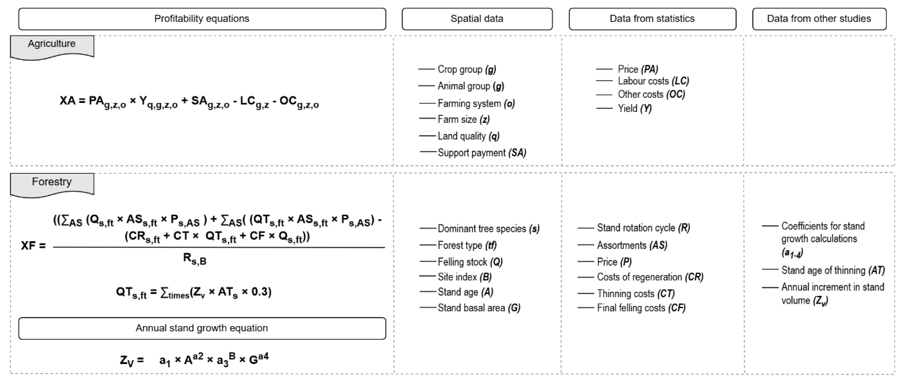
Figure 2.
Average profitability in agricultural land use (EUR/ha).
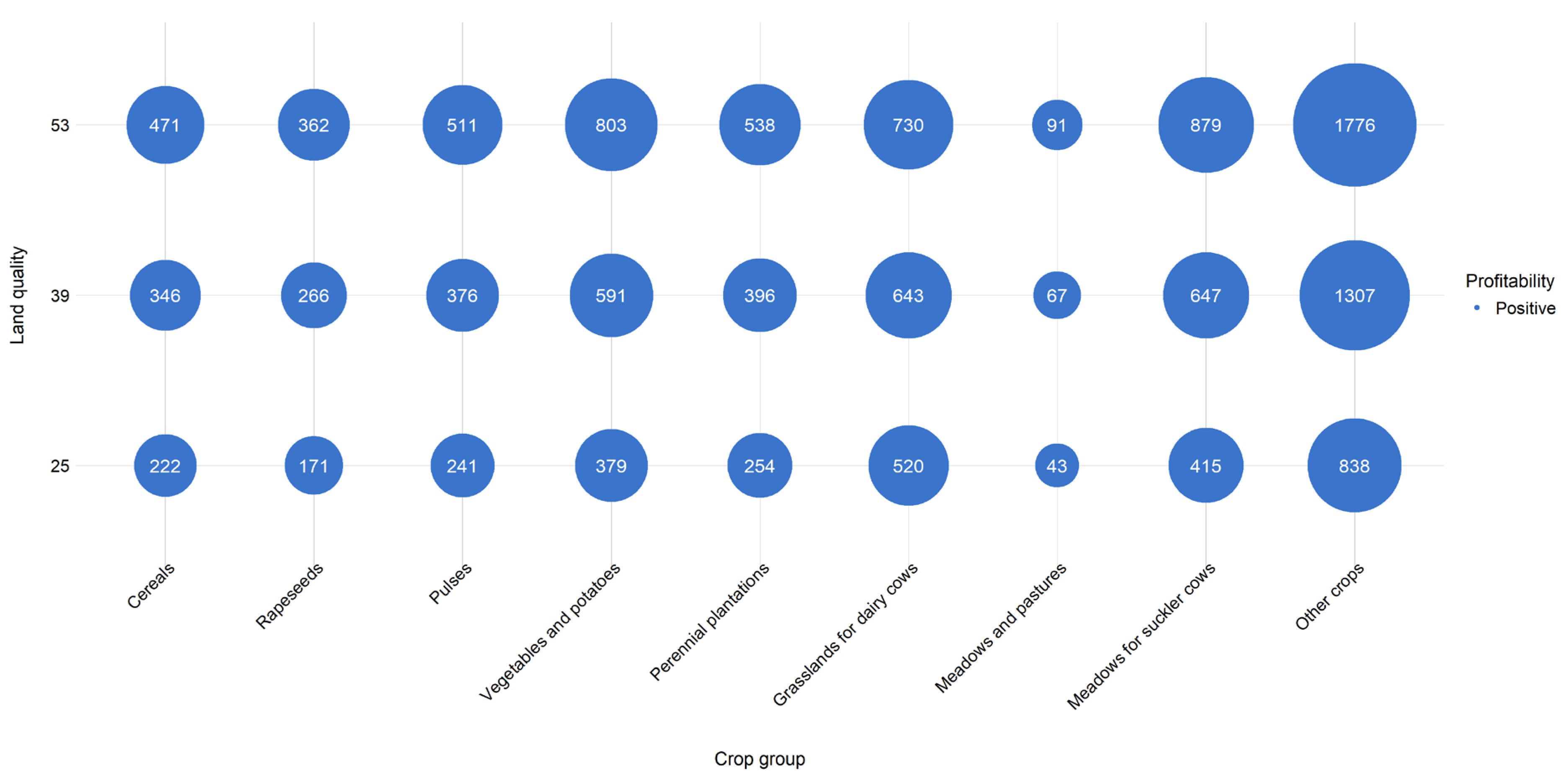
Figure 3.
Average profitability in agriculture across different crop groups and farm size categories (EUR/ha).
Figure 3.
Average profitability in agriculture across different crop groups and farm size categories (EUR/ha).
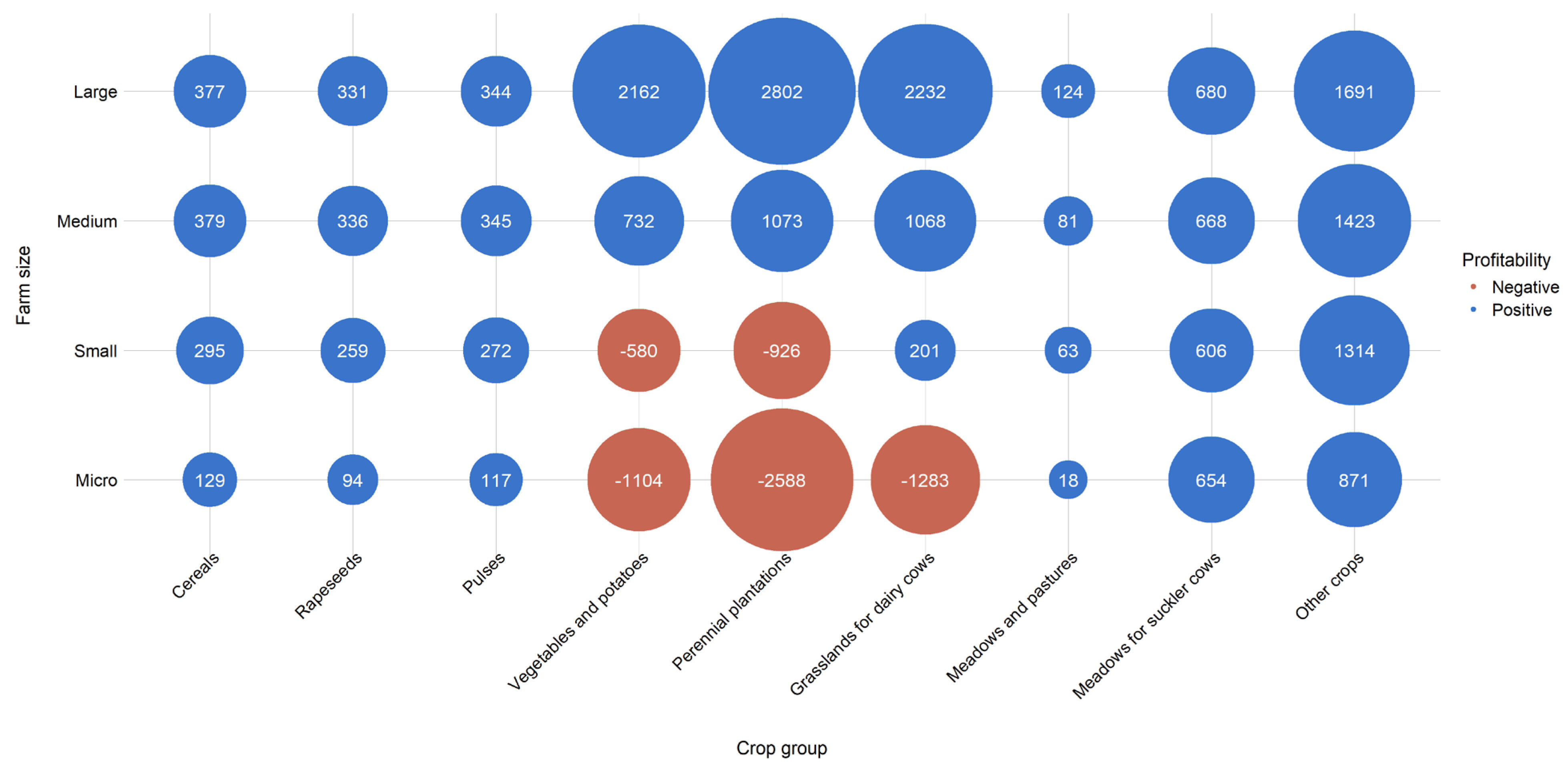
Figure 4.
Average profitability in forest land use (EUR/ha).
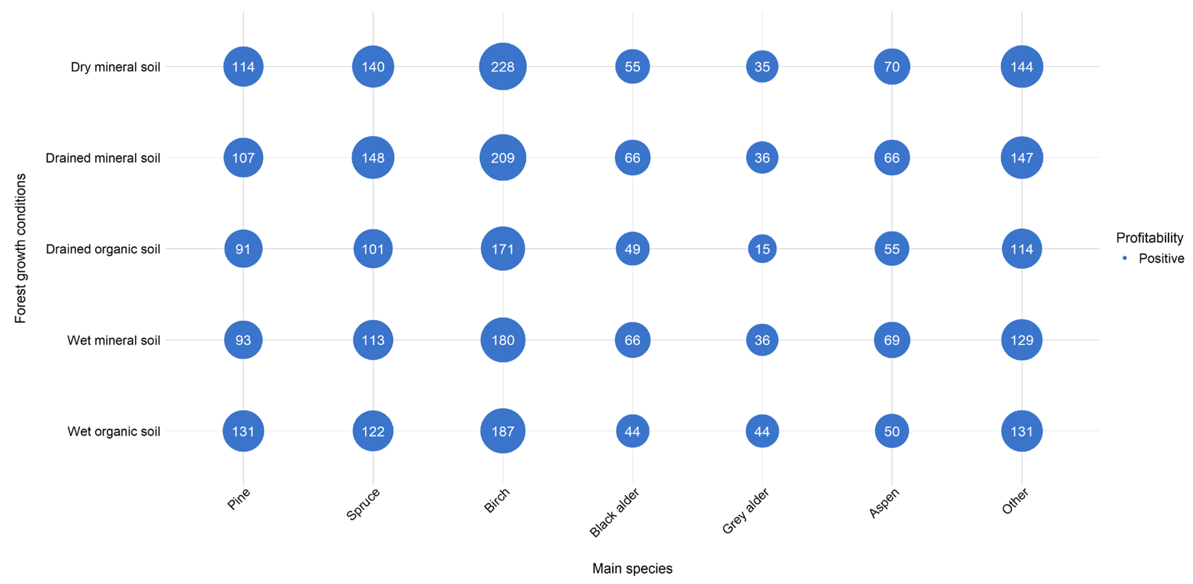
Figure 5.
Spatial distribution of agricultural profitability in Latvia (EUR/ha).
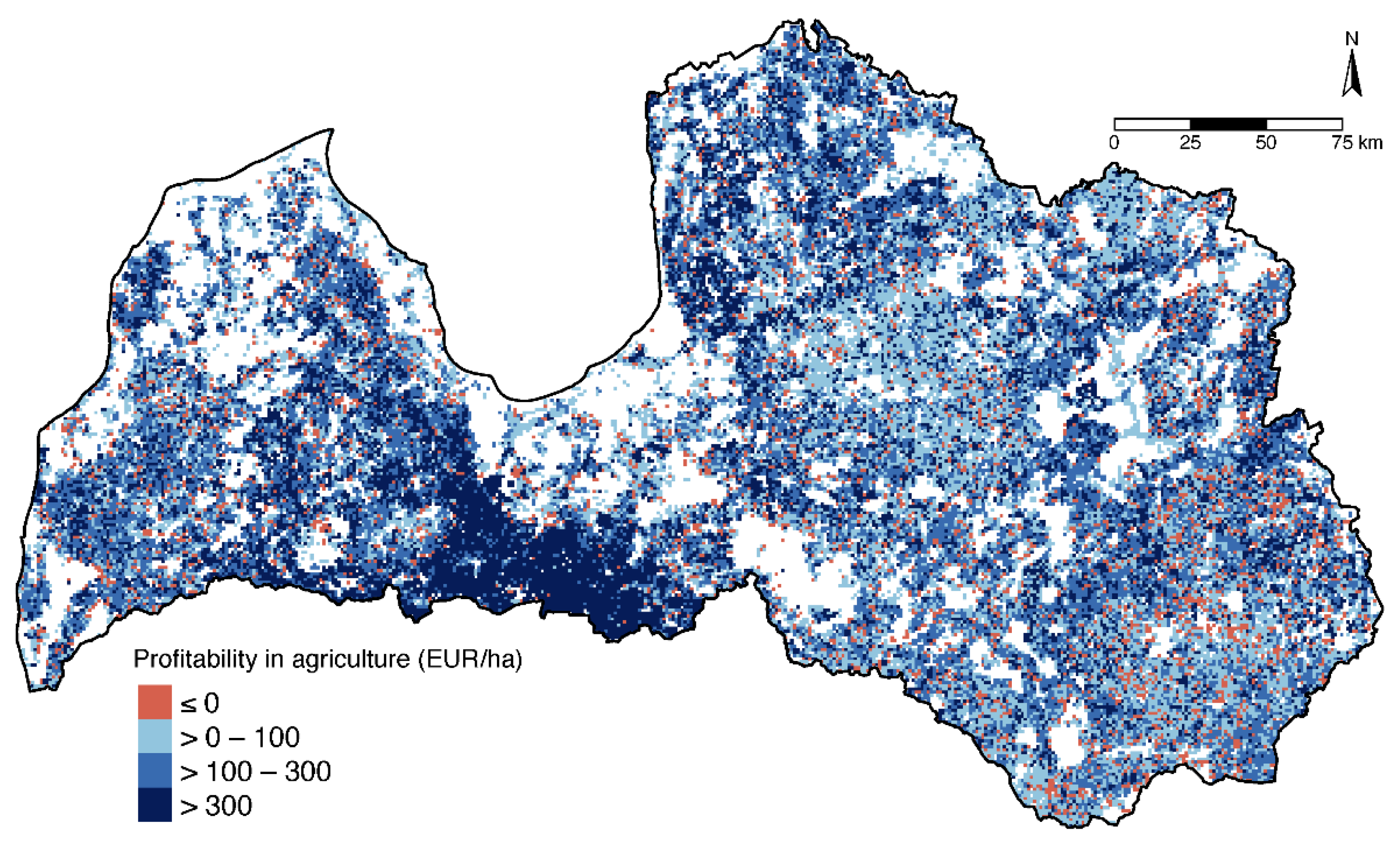
Figure 6.
Spatial distribution of forestry profitability in Latvia (EUR/ha).
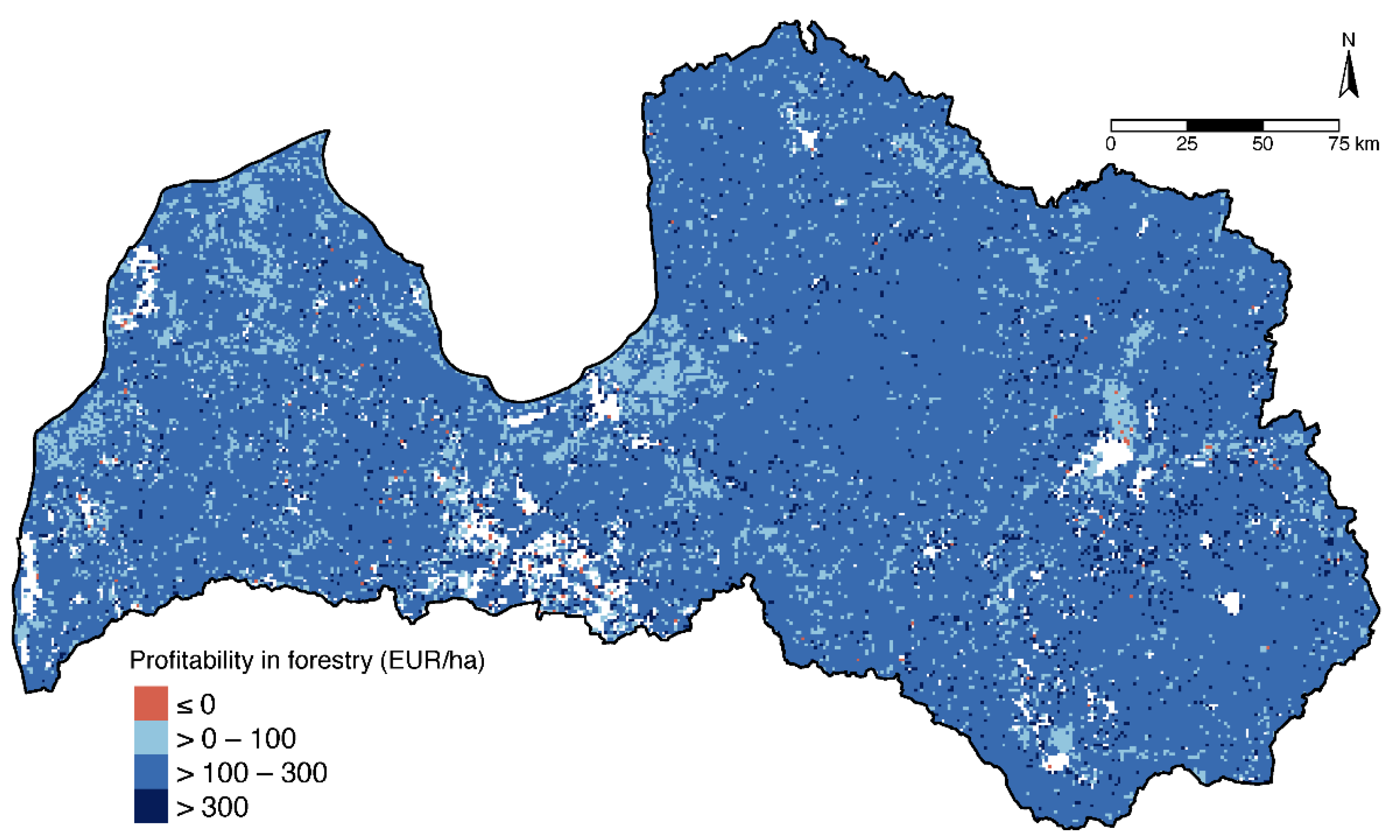
Disclaimer/Publisher’s Note: The statements, opinions and data contained in all publications are solely those of the individual author(s) and contributor(s) and not of MDPI and/or the editor(s). MDPI and/or the editor(s) disclaim responsibility for any injury to people or property resulting from any ideas, methods, instructions or products referred to in the content. |
© 2025 by the authors. Licensee MDPI, Basel, Switzerland. This article is an open access article distributed under the terms and conditions of the Creative Commons Attribution (CC BY) license (http://creativecommons.org/licenses/by/4.0/).
Copyright: This open access article is published under a Creative Commons CC BY 4.0 license, which permit the free download, distribution, and reuse, provided that the author and preprint are cited in any reuse.


