Spectral Clustering for Interdisciplinary Research: From Graph Theory to RNA-seq Data Analysis

1. The Laplacian Differential Operator

The Laplacian operator is ubiquitous in multivariable calculus as well as in Physics and Engineering. The aim of this section is to give some intuition of the continuous Laplacian to guide our thinking when we eventually define such an operator on graphs where it will become a discrete operator.

Given a function $f:I\subset \mathbb{R}⟶\mathbb{R}$, the Laplacian $\Delta f$ of f is the second derivative $f^{\prime \prime }$ of f, and plays a role when one wants to study its variations (extrema), or the curvature of its graph. However, it has another interpretation: the Laplacian of f is a measure of how much f deviates from its mean value. Considering a ball $[a-\epsilon ,a+\epsilon ]\subset I$ centered on a and with radius $\epsilon >0$, the mean value of f on the ball is defined by:

$$\overline{f}\left(a\right)={\displaystyle \frac{1}{2\epsilon }}{\int }_{a-\epsilon }^{a+\epsilon }f\left(x\right)\mathrm{d}x.$$

Performing a Taylor expansion of f around a we have for any $x\in ]a-\epsilon ,a+\epsilon [$:

$$f\left(x\right)=f\left(a\right)+f^{\prime }\left(a\right)x+{\displaystyle \frac{f^{\prime \prime }\left(a\right)}{2}}{x}^2+{\displaystyle \frac{f^{\prime \prime \prime }\left(a\right)}{6}}{x}^3+O\left(x^4\right),$$

so, after integrating and rearranging the expression, we obtain:

$$\Delta f\left(a\right)=f^{\prime \prime }\left(a\right)={\displaystyle \frac{12}{{\epsilon }^2}}\left(\overline{f}\left(a\right)-f\left(a\right)\right)+O\left({\epsilon }^2\right).$$

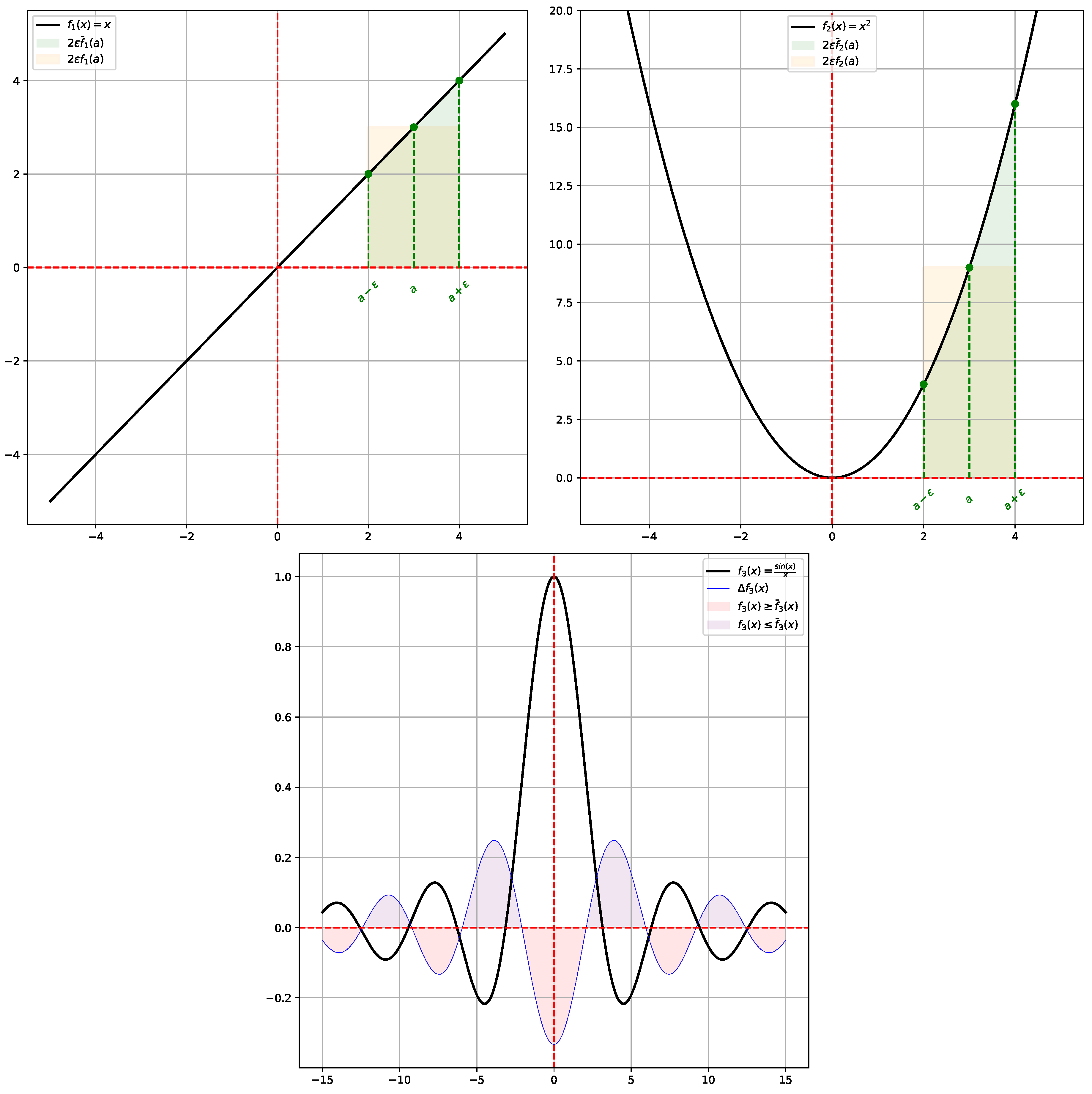
Therefore, if $\Delta f\left(a\right)>0$, the function f in a is lower than its average value $\overline{f}\left(a\right)$, and vice versa. So, essentially $\Delta f\left(a\right)$ measures the deviation of $f\left(a\right)$ from its mean value $\overline{f}\left(a\right)$, see Figure 1 for an illustration.

In the multivariate case, we look at a function $f:\Omega \subset {\mathbb{R}}^n\to \mathbb{R}$, and the Laplacian $\Delta f$ of f is the function defined for all $x\in \Omega$ by:

$$\Delta f\left(x\right)=\sum _{i=1}^n{\displaystyle \frac{{\partial }^{2}f}{\partial x_i^2}}\left(x\right)=\mathrm{div}(\nabla f)\left(x\right),$$

where $\nabla f=\left({\displaystyle \frac{\partial f}{\partial x_1}},\dots ,{\displaystyle \frac{\partial f}{\partial x_n}}\right)$ is the usual gradient of f (so a vector field) and $\mathrm{div}\left(X\right)={\sum }_{i=1}^n{\displaystyle \frac{\partial X_i}{\partial x_i}}$ the usual divergence of a vector field $X=(X_1,\dots ,X_n)$ (so a scalar field); both are also important differential operators in multivariable calculus. So, the Laplacian of a function is actually a measure of compression/expansion of its gradient vector field. But what is more interesting to us is that the previous interpretation of the Laplacian still holds in higher dimensions:

$\Delta f\left(a\right)$ measures the deviation of $f\left(a\right)$ from its mean value $\overline{f}\left(a\right)$ over a ball centered on a and of radius $\epsilon$:

$$\Delta f\left(a\right)\propto \left(\mathrm{average}\mathrm{of}f\mathrm{around}a\right)-\left(\mathrm{value}\mathrm{of}f\mathrm{at}a\right).$$

See [1] for more details on the multidimensional approach.

2. Discretizing the Laplacian Operator

In this section, we take a small detour in numerical analysis to continue to build our intuition. Finite differences is a mathematical method used to discretize partial differential equations (PDE) on regular grids. As the Laplace operator appears in various PDE, such as the Poisson equation and the heat equation, finite differences for the Laplacian operator were developed accordingly to discretize it.

Let us first consider the single variable case. Given a function $f:I\to \mathbb{R}$, we can write down the following two Taylor expansions of f (others are possible):

$$\begin{array}{c}f(x+h)=f\left(x\right)+f^{\prime }\left(x\right)h+f^{\prime \prime }\left(x\right){\displaystyle \frac{h^2}{2}}+O\left(h^3\right),\\ f(x-h)=f\left(x\right)-f^{\prime }\left(x\right)h+f^{\prime \prime }\left(x\right){\displaystyle \frac{h^2}{2}}+O\left(h^3\right).\end{array}$$

Then, combining them we obtain the following approximation for the Laplacian:

$$\Delta f\left(x\right)=f^{\prime \prime }\left(x\right)={\displaystyle \frac{f(x-h)-2f\left(x\right)+f(x+h)}{h^2}}+O\left(h\right).$$

Suppose now that $I=[a,b]$ is discretized into a regular 1D grid $I_h={\left\{x_i\right\}}_{1\le i\le N}$ such that $x_1=a$, $x_N=b$ and the distance between two consecutive points (the so-called resolution of the grid) is h. The function f is then represented (discretized) on $I_h$ as the vector $\mathit{f}={\left(f_i\right)}_{1\le i\le N}\in {\mathbb{R}}^N$, and each $f_i$ represents the value that takes f at the point (node) $x_i$. In this setting, the preceding formula says that we can approximate the function $\Delta f$ on I by the discrete function $L\left(f\right)$ on $I_h$ according to the formula (with the $-2$ coefficient located at the i-th index in the matrix product)):

$$L{\left(f\right)}_i={\displaystyle \frac{f_{i-1}-2f_i+f_{i+1}}{h^2}}={\displaystyle \frac{1}{h^2}}\left[\begin{array}{ccccccc}0& \dots & 1& -2& 1& \dots & 0\end{array}\right]\mathit{f},$$

valid at any inner point of the grid $I_h$. For $i=1$ we remove the term $x_{i-1}$, and for $i=N$ we remove $x_{i+1}$ simply because these terms do not exist in these corner cases. The error due to this approximation is bounded by the resolution h of the grid. All in all, we can write $L\left(f\right)$ as the matrix product $L\mathit{f}$ where L is the sparse matrix given by:

$$L=\left[\begin{array}{ccccc}-2& 1& 0& \dots & 0\\ 1& -2& 1& \dots & 0\\ ⋮& \ddots & \ddots & \ddots & 0\\ 0& \dots & 0& -2& 1\end{array}\right].$$

Finite differences for the Laplacian in multiple dimensions are available as well. Let us now consider a function of two variables $f:(x,y)\in \Omega \subset {\mathbb{R}}^2\mapsto f(x,y)\in \mathbb{R}$, and suppose $\Omega$ is a square than can be discretized into a regular 2D grid ${\Omega }_h={\left\{x_{i,j}\right\}}_{1\le i,j\le N}$ with both horizontal and vertical resolutions equal: $\Delta x=\Delta y=h$. The function f is then discretized into a matrix $\mathit{f}={\left(f_{i,j}\right)}_{1\le i,j\le N}\in {\mathbb{R}}^{N\times N}$, where $f_{i,j}$ represents the value of f at node $x_{i,j}$. Then using Taylor series we can for instance come up with the approximation:

$$\Delta f(x,y)={\displaystyle \frac{f(x-h,y)+f(x+h,y)-4f(x,y)+f(x,y-h)+f(x,y+h)}{h^2}}+O\left(h\right),$$

so that locally the Laplacian at a node $x_{i,j}$ is given by:

$$L{\left(f\right)}_{i,j}={\displaystyle \frac{f_{i-1,j}+f_{i+1,j}-4f_{i,j}+f_{i,j-1}+f_{i,j+1}}{h^2}},$$

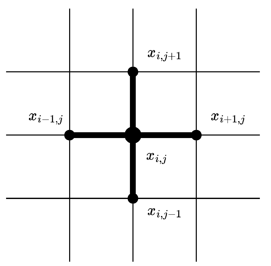
and it is possible after rearranging a little bit (by stacking the columns or the rows of $\mathit{f}$) to obtain a sparse matrix L that corresponds to the discrete Laplacian in two dimensions. See Figure 2 for a visualization of the so-called stencil that defines the local neighborhood used to create a discrete Laplacian by using five points.

To summarize:

• The discrete version of $\Delta f\left(x\right)$ clearly measures the deviation of $f\left(x\right)$ from its average over a small grid neighborhood; we still have (in 2D):

  $${\left(L\mathit{f}\right)}_{i,j}\propto \left(\mathrm{average}\mathrm{of}\mathit{f}\mathrm{around}{x}_{i,j}\right)-\left(\mathrm{value}{\mathit{f}}_{i,j}\mathrm{of}\mathit{f}\mathrm{at}{x}_{i,j}\right).$$
• The discretized Laplacian L is now a matrix, reflecting on the linear nature of the continuous operator.

3. The Ubiquitous Nature of Graph Structures

In this section we review what a graph is and what are some applications of graph theory in applied mathematics and Science in general.

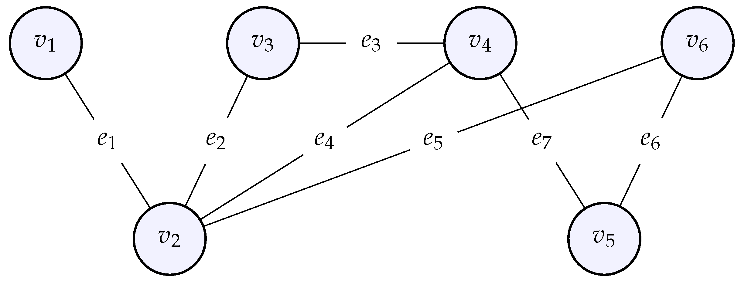
A graph is a mathematical structure, capable of modeling relationships among entities that compose the graph. A graph $G=(V,E)$ consists of a set of vertices (nodes)$V=\{v_1,\dots ,v_N\}$ and a set of edges$E=\{e_1,\dots ,e_M\}$ that connect these vertices. The nodes correspond to the entities, whose relationships are modeled by the edges. Below is an example of a graph with 6 nodes $v_1,\dots ,v_6$ and 7 vertices $e_1,\dots ,e_7$.

Figure 3. An example of an undirected graph with six nodes $v_1,\dots ,v_6$ and seven edges $e_1,\dots ,e_7$.

Figure 3. An example of an undirected graph with six nodes $v_1,\dots ,v_6$ and seven edges $e_1,\dots ,e_7$.

Such a mathematical structure allows one to encode any system whose parts are interdependent rather than isolated, although a graph can also be composed of nodes not connected to any other node. The distances between the nodes are not important in our setting, we are rather interested in the relationships between the nodes, who is connected to whom, which constitutes the so-called topology of the graph. Note also that the regular grids described in the previous section are actually a certain type of graph for which the geometry (the precise location of the nodes in the discretized domain) is important as well. When there is a priori no orientation for the edges, the graph is said to be undirected by opposition to a directed graph. Later, we will also add weights to the edges, in that case we speak of a weighted graph.

Graphs are used in various fields, especially those studying network-based systems, like social networks, electrical circuits, or transportation and supply chain networks, as they offer a way to formalize the connectivity and influence between subsystems. In Bioinformatics and Computational Biology, graphs appear in a number of topics, such as gene regulatory networks [2,3] and single cell RNA sequencing data analysis [4]. Graph theory is a subfield of Mathematics that provides tools to analyze graphs, detect patterns and make predictions for these structures.

4. Various Graph Laplacians

After obtaining a good intuition of the Laplacian operator in a continuous setting (Section 1) and also in a particular discrete setting (Section 2), in this section we define the Laplacian operator on a graph. Actually, as we will see, there are several possible definitions, according to what we actually want to do. Afterwards, like with any operator in applied mathematics, we can use linear algebra to get insights and retrieve information that has been encoded. This is the main idea behind spectral graph theory: investigate the Laplacian of a graph (or other related matrices) to gain insights into the internal organization of the data. We refer the reader to [5], chapter 1] as well as [6] for more details.

A function on the graph is just the association of a number to each node of the graph. Therefore, it can be represented as a vector $f=(f_1,\dots ,f_N)\in {\mathbb{R}}^N$. We will also encounter functions on the edges of the graph. They are represented by vectors $g=(g_1,\dots ,g_M)\in {\mathbb{R}}^M$ and correspond rather to the concept of vector fields on the graph, as we associate a value to each possible direction.

4.1. The Gradient of a Function

As we are going to define the graph Laplacian as the divergence of the gradient, let’s first introduce the gradient of a function on a graph. In the usual Euclidean space ${\mathbb{R}}^2$, the gradient of a function gives the variations of the function in the direction given by $e_1=(1,0)$ and $e_2=(0,1)$, which are available at each point $(x,y)$. However, unlike continuous Euclidean space, a graph offers no privileged directions at a given node. Instead, the available directions are strictly defined by the edges incident to that node. To this end, we give an orientation to the edges: we simply sort the nodes by increasing order, and say that an edge e goes from node u to node v if and only if the index of u is less than the index of v. Now, given a node $v_i\in V$, and an edge $e=v_i\to v_j\in E$ starting at this node, the variation of the function f into the direction given by that edge is simply $f_j-f_i$. We can do so for all edges adjacent to this node $v_i$, which basically represents the gradient of f at the node $v_i$. Then, we can repeat this process for all nodes. All in all, we can present this information by using a matrix, the so-called incidence matrixK, of size $\left|E\right|\times \left|V\right|$, whose coefficients are defined by:

$$K_{e,v}=\left\{\begin{array}{c}1\mathrm{if}e\mathrm{starts}\mathrm{at}v\hfill \\ -1\mathrm{if}e\mathrm{ends}\mathrm{at}v\hfill \\ 0\mathrm{otherwise}\hfill \end{array}\right..$$

Essentially, the incident matrix tells if a certain node is the source or the end of an edge, or neither. For the example graph above, the incidence matrix reads:

$$K=\left[\begin{array}{cccccc}1& -1& 0& 0& 0& 0\\ 0& 1& -1& 0& 0& 0\\ 0& 0& 1& -1& 0& 0\\ 0& 1& 0& -1& 0& 0\\ 0& 1& 0& 0& 0& -1\\ 0& 0& 0& 0& 1& -1\\ 0& 0& 0& 1& -1& 0\end{array}\right],$$

where rows correspond to the edges $e_1,\dots ,e_7$ and the columns correspond to the nodes $v_1,\dots ,v_6$. Then, computing the gradient of f amounts to compute the matrix-vector product $Kf$:

$$Kf=\left[\begin{array}{cccccc}1& -1& 0& 0& 0& 0\\ 0& 1& -1& 0& 0& 0\\ 0& 0& 1& -1& 0& 0\\ 0& 1& 0& -1& 0& 0\\ 0& 1& 0& 0& 0& -1\\ 0& 0& 0& 0& 1& -1\\ 0& 0& 0& 1& -1& 0\end{array}\right]\left[\begin{array}{c}{f}_1\\ f_2\\ f_3\\ f_4\\ f_5\\ f_6\end{array}\right]=\left[\begin{array}{c}{f}_1-f_2\\ f_2-f_3\\ f_3-f_4\\ f_2-f_4\\ f_2-f_6\\ f_5-f_6\\ f_4-f_5\end{array}\right],$$

so that each row of the result corresponds to the gradient of the function f in the direction given by the edge associated to that row. Notice that the output is then of size M, that is the gradient of a function on the nodes is a function on the edges of the graph.

4.2. The Divergence of a Vector Field

Now we also need an operator on the graph that mimics what the divergence of a vector field does in the continuous case, which represents the net flow of this vector field that goes in and out at a point. For us, the input will be a function on the edges of the graph and the output will be a function on the nodes of the graph. Such input somehow already represents the flow of an hypothetical vector field, therefore we can define the divergence as simply the sum of all the function components, with a sign according to whether the edge is ingoing or outgoing at that node. For example, given a function $g\in {\mathbb{R}}^7$ on the edges of the example graph above, the divergence of g at the node $v_4$ is $g_3+g_4-g_7$. It turns out that doing so for all the components of g we find that the divergence of g is actually $-K^{\mathsf{T}}g$:

$$-K^{\mathsf{T}}g=\left[\begin{array}{ccccccc}-1& 0& 0& 0& 0& 0& 0\\ 1& -1& 0& -1& -1& 0& 0\\ 0& 1& -1& 0& 0& 0& 0\\ 0& 0& 1& 1& 0& 0& -1\\ 0& 0& 0& 0& 0& -1& 1\\ 0& 0& 0& 0& 1& 1& 0\end{array}\right]\left[\begin{array}{c}{g}_1\\ g_2\\ g_3\\ g_4\\ g_5\\ g_6\\ g_7\end{array}\right]=\left[\begin{array}{c}-g_1\\ g_1-g_2-g_4-g_5\\ g_2-g_3\\ g_3+g_4-g_7\\ g_7-g_6\\ g_5+g_6\end{array}\right],$$

so that each row of the result corresponds to the divergence at a node in the graph.

4.3. The Laplacian of a Function

Finally, since the continuous Laplacian is given by the divergence of the gradient, the graph Laplacian L of a function $f\in {\mathbb{R}}^N$ is simply defined to be the function $Lf:=-K^{\mathsf{T}}Kf$, which mimics perfectly the relation $\Delta f=-{\nabla }^{★}\nabla f$ of calculus, where ${\nabla }^{★}$ is the dual of the gradient with respect to the integrated Euclidean dot product, which is nothing less than minus the divergence according to the divergence theorem, assuming no boundary. As an example, let us compute ${\left(Lf\right)}_2$, which is the value of the graph Laplacian of f at the node $v_2$ in the example graph above:

$$\begin{array}{cc}\hfill {\left(Lf\right)}_2=& -{\left(K^{\mathsf{T}}g\right)}_2{|}_{g=Kf}\hfill \\ \hfill =& (f_1-f_2)-(f_2-f_3)-(f_2-f_4)-(f_2-f_6)\hfill \\ \hfill =& (f_1+f_3+f_4+f_6)-4f_2.\hfill \end{array}$$

Note that it follows from the definition of the graph Laplacian that it is symmetric.

• The graph Laplacian L is a symmetric matrix.
• It measures the deviation of a function on the nodes from its average over adjacent nodes; we have again:

  $${\left(Lf\right)}_i\propto \left(\mathrm{average}\mathrm{of}f\mathrm{over}\mathrm{adjacent}\mathrm{nodes}\mathrm{to}{v}_i\right)-\left(\mathrm{value}{f}_i\mathrm{of}f\mathrm{at}\mathrm{node}{v}_i\right).$$

4.4. Another Expression of the Graph Laplacian

The graph Laplacian admits another expression that uses two other matrices. The degree matrix of the graph is the diagonal matrix D with the i-th element on its diagonal being the degree $deg\left(v_i\right)$ of the node $v_i\in V$, that is, how many adjacent edges to $v_i$ are there. Therefore it is of size $N\times N$. Second, the adjacency matrix is yet another matrix A, also of size $N\times N$, defined by:

$$A_{i,j}=\left\{\begin{array}{c}1\mathrm{if}\mathrm{there}\mathrm{is}\mathrm{an}\mathrm{edge}\mathrm{between}{v}_i\mathrm{and}{v}_j\hfill \\ 0\mathrm{otherwise}\hfill \end{array}\right..$$

Remark that $D_i={\sum }_{j\in \mathcal{N}\left(i\right)}{A}_{i,j}$ by definition of the degree, where $\mathcal{N}\left(i\right)$ denotes the set of neighbors of the i-th node. We are going to show that the graph Laplacian L is equal to $A-D$, that is, $-K^{\mathsf{T}}K=A-D$. To show this equality, we work coefficient by coefficient. Recall from linear algebra that ${\left(AB\right)}_{i,j}=A_{i,•}{B}_{•,j}$, where $A_{i,•}$ denotes the i-th row of the matrix A, and $B_{•,j}$ the j-th column of the matrix B. We have

$${(-K^{\mathsf{T}}K)}_{i,j}=-{\left(K^{\mathsf{T}}\right)}_{i,•}{K}_{•,j}=-{\left(K_{•,i}\right)}^{\mathsf{T}}{K}_{•,j},$$

therefore:

• For $i=j$, ${(-K^{\mathsf{T}}K)}_{i,i}=-{\left(K_{•,i}\right)}^{\mathsf{T}}{K}_{•,i}=-deg\left(v_i\right)$, because all the $-1$ get multiplied with the same $-1$, and similarly for the 1;
• For $i\ne j$, $K_{•,i}$ relates to edges adjacent to $v_i$ while $K_{•,j}$ relates to edges adjacent to $v_j$. Therefore, the product ${\left(K_{•,i}\right)}^{\mathsf{T}}{K}_{•,j}$ takes into account edges that are adjacent on both $v_i$ and $v_j$ (because otherwise a zero will zero out the contribution of an adjacent edge to one node only), which are at most one. For such an edge, we will always obtain $-1$ because $v_i$ is either the start or end of that edge, while $v_j$ would be the opposite.

The $N\times N$ matrix L known as the graph Laplacian admits the following expressions:

$$L=-K^{\mathsf{T}}K=A-D,$$

where K is the $M\times N$ incidence matrix, A is the $N\times N$ adjacency matrix and D is the $N\times N$ degree matrix. With this expression it is easy to obtain the following one (that we already had a glimpse into):

$${\left(Lf\right)}_i=\sum _{j\in \mathcal{N}\left(i\right)}(f_j-f_i),$$

where $j\in \mathcal{N}\left(i\right)$ means that we are looking at nodes $v_j$ that are adjacent to node $v_i$. This formula clearly states that the graph Laplacian of a function at a certain node measures the deviation between its average on a direct neighborhood of the node and the value of the function at that node.

In the same way as in multivariable calculus, the Laplacian operator we defined is negative-definite. Indeed we have for any $f\in {\mathbb{R}}^N$:

$$f^{\mathsf{T}}Lf=-f^{\mathsf{T}}{K}^{\mathsf{T}}Kf=-{\parallel Kf\parallel }_2^2\le 0.$$

Therefore, in order to have positive eigenvalues later on, in everything that follows we will use the opposite of the operator we defined. From now on we set $L=K^{\mathsf{T}}K=D-A$.

4.5. Variants of the Graph Laplacian

We introduced perhaps the most elementary version of the graph Laplacian that mimics the Laplacian found in multivariable calculus. It is sometimes called the combinatorial Laplacian or the unnormalized Laplacian. There are variants though, depending on the analysis we wish to conduct. Below are some pointers to other variations of the initial definition we gave.

• The incidence matrix is often defined as the transpose of the matrix we used, so the combinatorial Laplacian is then $L=K{K}^{\mathsf{T}}$, but it is now positive-definite, as we explained in the previous box.
• A very important case is when the graph is weighted, meaning that to an edge between nodes $v_i$ and $v_j$ is associated a positive real number $w_{i,j}$, called the weight of the edge. Negative weights are also possible but the generalization of the Laplacian in this case can go into different directions, see for instance [7] and [8]. In the case of a weighted graph, weights are directly incorporated naturally in the adjacency matrix A. The (positive-definite) graph Laplacian is then $L=D-A=KW{K}^{\mathsf{T}}$, with W a $M\times M$ diagonal matrix containing all the weights. We still obtain a symmetric positive-definite graph Laplacian.
• Normalizations: it is sometimes important to normalize the diagonal entries of the graph Laplacian to 1, for instance, in order to interpret certain quantities in terms of probabilities as we will see in Section 7. As mentioned before, the diagonal of the graph Laplacian consists of the degrees of the different nodes. Normalizing the Laplacian consists of decreasing the influence of the degree of a node (i.e., its total connectivity). Therefore, normalizing the Laplacian naturally introduces the pseudo-inverse of the degree matrix, $D^{+}$, which is necessary because some nodes may have zero connections. This operator is used to define the so-called random walk Laplacian, $L_{\mathrm{rw}}:=D^{+}L=I_N-D^{+}A$. Note, however, that this matrix is not symmetric anymore, which is an important property, for instance, if we want to guarantee that eigenvectors form an orthonormal basis. In the case we want a symmetric normalized Laplacian, $L_{\mathrm{sym}}:={\left(D^{+}\right)}^{{\displaystyle \frac{1}{2}}}L{\left(D^{+}\right)}^{{\displaystyle \frac{1}{2}}}=I_N-{\left(D^{+}\right)}^{{\displaystyle \frac{1}{2}}}A{\left(D^{+}\right)}^{{\displaystyle \frac{1}{2}}}$ will do. This variant is sometimes called the symmetric random walk Laplacian.

5. Eigenvalues and Eigenvectors of the Laplacian

In this section, we explore how eigenvalues and eigenvectors of the graph Laplacian relate to the structure of the graph. As a positive-definite matrix, the graph Laplacian has positive eigenvalues. If in addition it is symmetric (remember that certain normalizations break the symmetry), then the associated eigenvectors are orthogonal to each other. Because eigenvectors of the Laplacian can actually be considered as functions on the nodes of the graph, we will use the term eigenfunctions instead. Here is an outlook of what we are going to observe:

• The smaller the eigenvalue, the smoother the eigenfunction (meaning, the less variations). Indeed let $\lambda$ be an eigenvalue and f be the associated eigenvector of L. We can always normalize f without loss of generality, so we will suppose $f^{\mathsf{T}}f=1$. Then

  $$\lambda =f^{\mathsf{T}}Lf=\sum _{i,j\in \mathcal{N}\left(i\right)}{(f_j-f_i)}^2.$$

  (1)
  Therefore, when an eigenvalue is high, it can essentially be for two reasons. Either the graph has lots of connected nodes, corresponding to a lot of terms in the above sum even if the variations $f_j-f_i$ are not large (like in the cyclic graph example below), or there are a few nodes that are a lot more connected than the others (like in the star graph example below) so the sum has less terms but the variations $f_j-f_i$ are larger. For clarity, let’s derive expression (1):

  $$\begin{array}{cc}\hfill f^{\mathsf{T}}Lf& =\sum _i{D}_i{f}_i^2-\sum _{i,j}{A}_{i,j}{f}_i{f}_j\hfill \\ \hfill & =\sum _{i,j}{A}_{i,j}{f}_i^2-\sum _{i,j}{A}_{i,j}{f}_i{f}_j\hfill \\ \hfill & ={\displaystyle \frac{1}{2}}\sum _{i,j}{(f_j-f_i)}^2\hfill \\ \hfill & =\sum _{i,j\in \mathcal{N}\left(i\right)}{(f_j-f_i)}^2,\hfill \end{array}$$

  where we used the symmetry of the adjacency matrix A from the second to the third line.
• The multiplicity of the zero eigenvalue corresponds to the number of connected components of the graph.
• The eigenfunction of the first non null eigenvalue is the called the Fiedler vector and partitions the graph in two.

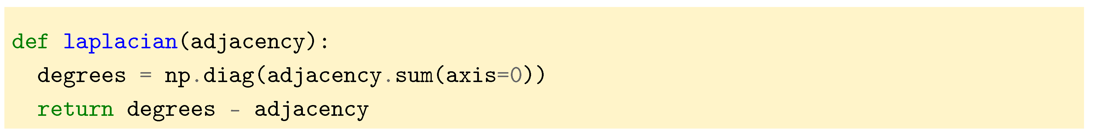
But first we need a way to define a graph in terms of code and compute its Laplacian. We choose to represent the graph by its adjacency matrix A. Unless specified, we will work with non weighted graphs in this section. From the adjacency matrix it is then possible to compute the degree matrix D by summing the columns of A. Then, as we have seen in the previous section, the combinatorial graph Laplacian is $L=D-A$.

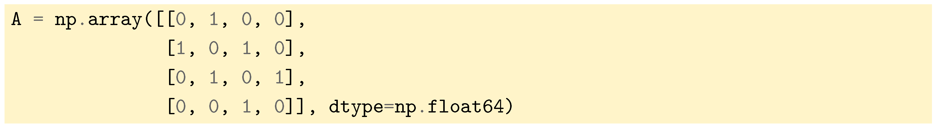
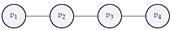
5.1. Computations for a Line Graph

Let us now compute the Laplacian, eigenvalues and eigenfunctions for a line graph, whose adjacency matrix is defined by:

Figure 4. The line graph whose adjacency matrix was given above.

Figure 4. The line graph whose adjacency matrix was given above.

Now by typing , we are able to compute the Laplacian of the line graph:

$$L=\left[\begin{array}{cccc}1& -1& 0& 0\\ -1& 2& -1& 0\\ 0& -1& 2& -1\\ 0& 0& -1& 1\end{array}\right].$$

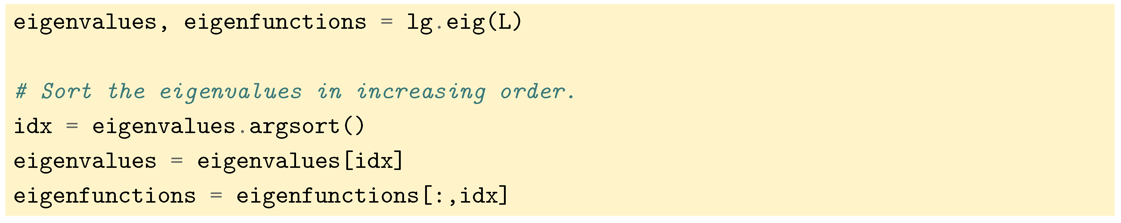
Then, the eigenvalues and eigenvectors are computed with the SciPy routine that leverages Singular Value Decomposition (SVD1). After this computation is done, eigenvalues and the corresponding eigenvectors are sorted in increasing order.

To have a simple output of this eigenvalues, we format them as follows and take the real part (SciPy do all computations with complex numbers):

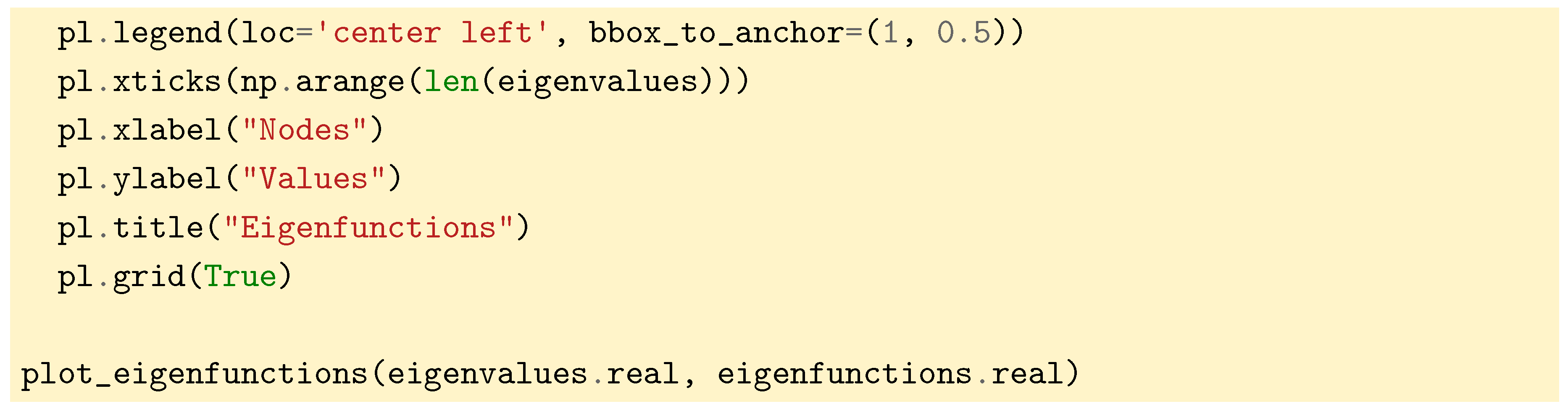
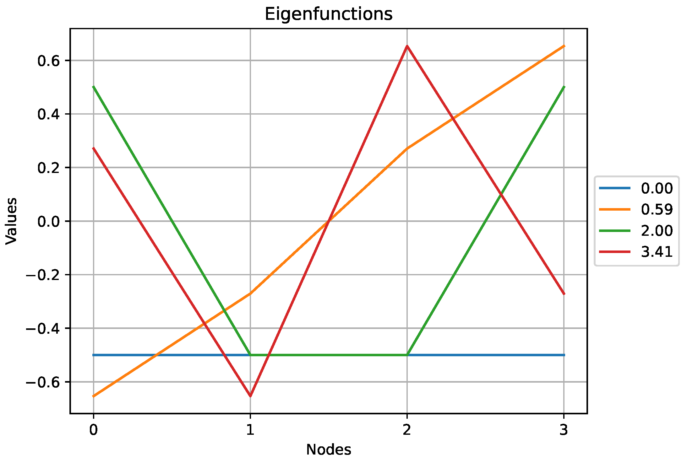
We then obtain that the spectrum of L (the set of all eigenvalues of L) is $\{0,0.59,2,3.41\}$. We also plot the eigenfunctions against the different vertices of the graph with the help of the following function:

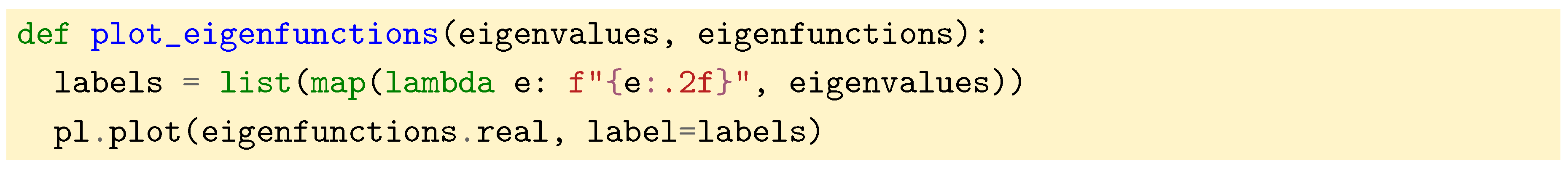
Figure 5. The eigenfunctions obtained for the line graph above. Note that the higher the eigenvalue, the higher the variations of the eigenfunction.

Figure 5. The eigenfunctions obtained for the line graph above. Note that the higher the eigenvalue, the higher the variations of the eigenfunction.

From this plot we see that the lower the value of the eigenvalue, the less variations in the corresponding eigenfunction. This is familiar to those readers who have practiced mechanics: the highest eigenvalues of the operator describing a system’s dynamics (it often involves a Laplacian or a discrete Laplacian) correspond to the largest vibrations of the system (see [9] and the seminal article [10]).

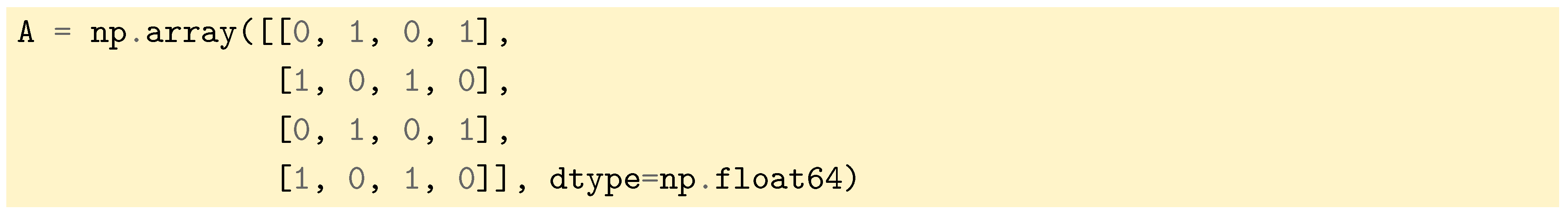
5.2. Computations for a Cyclic Graph

Let us define a cyclic graph with the following adjacency matrix:

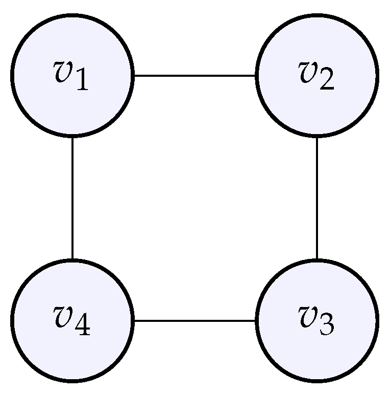
Figure 6. The cyclic graph whose adjacency matrix was given above.

Figure 6. The cyclic graph whose adjacency matrix was given above.

Figure 7. The eigenfunctions obtained for the cyclic graph above. Note that the two eigenfunctions associated to the eigenvalue $\lambda =2$ exhibit some symmetry.

Figure 7. The eigenfunctions obtained for the cyclic graph above. Note that the two eigenfunctions associated to the eigenvalue $\lambda =2$ exhibit some symmetry.

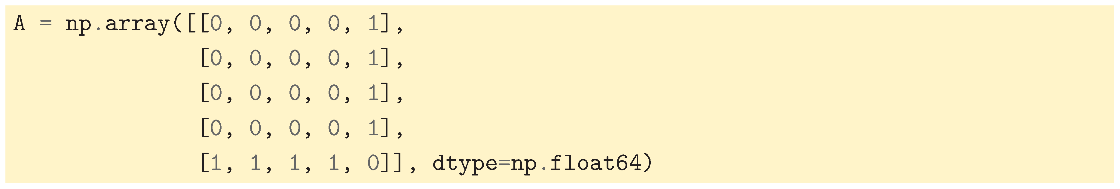
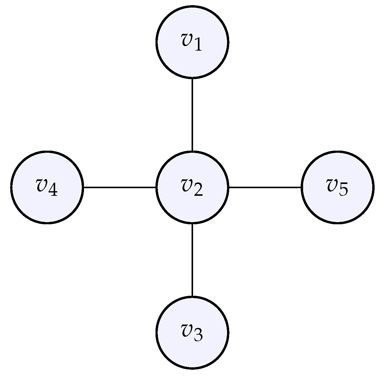
5.3. Computations for a Star Graph

The case of a star graph is also interesting, because it exhibits dissymmetry: one node at the center is connected to all others. For adjacency matrix we take:

Figure 8. The star graph whose adjacency matrix was given above.

Figure 8. The star graph whose adjacency matrix was given above.

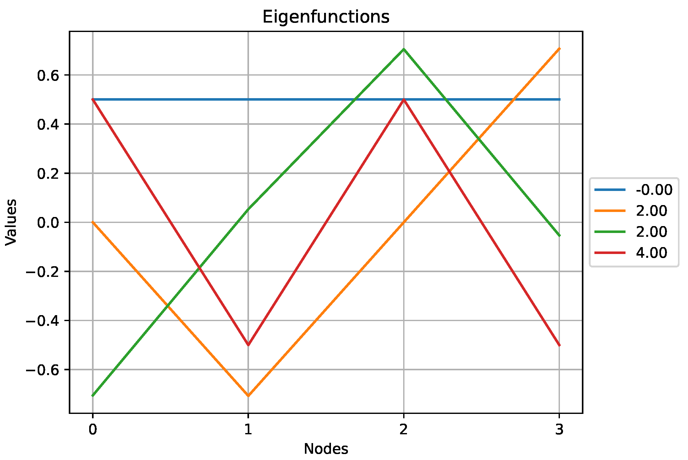
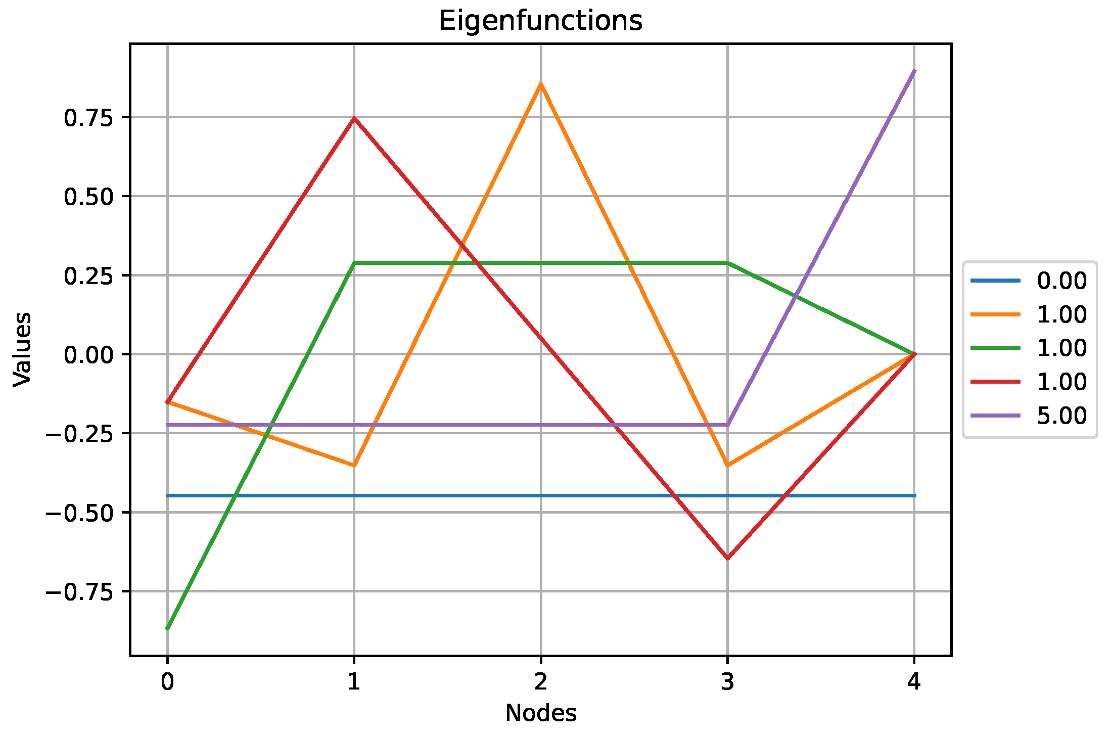
Figure 9. The eigenfunctions obtained for the star graph above.

Figure 9. The eigenfunctions obtained for the star graph above.

Here we observe that the eigenfunction associated with the highest eigenvalue, $\lambda =5$, does not exhibit a lot of variations compared to other eigenfunctions. Indeed, according to (1), the high value of $\lambda$ comes from the high degree of the central node which results in an eigenfunction that puts a lot of weight on this particular node.

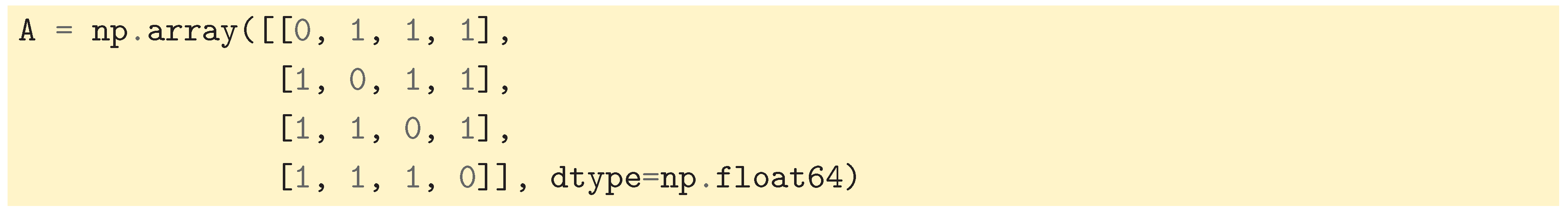
5.4. Computations with a Complete Graph

We will now observe that the more connected the graph is, the higher the eigenvalues are. Starting from 4 individual nodes (like with a cyclic graph before), we complete the graph so that each node is connected to all the others; we obtained a so-called complete graph whose adjacency matrix is given by:

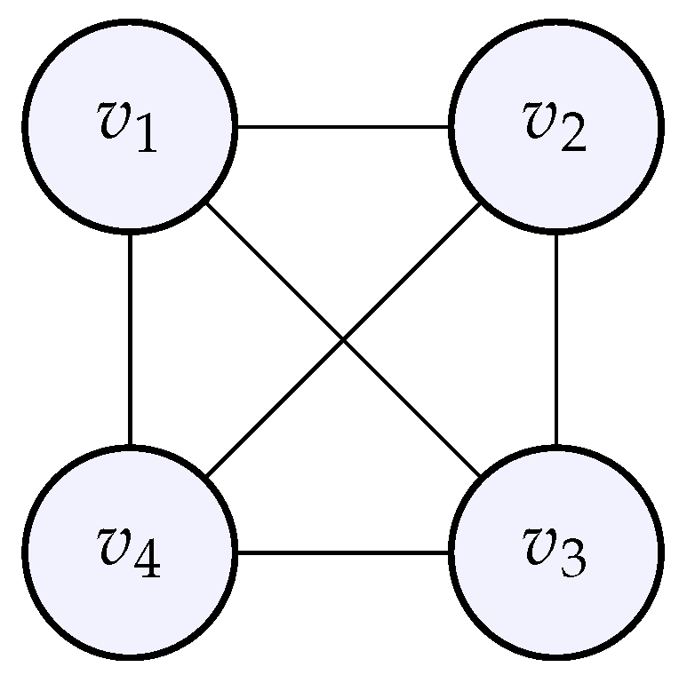
Figure 10. The complete graph whose adjacency matrix was given above.

Figure 10. The complete graph whose adjacency matrix was given above.

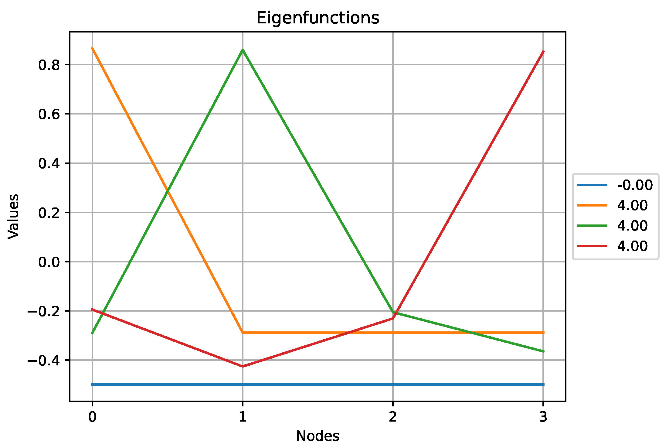
Figure 11. The eigenfunctions obtained for the complete graph above.

Figure 11. The eigenfunctions obtained for the complete graph above.

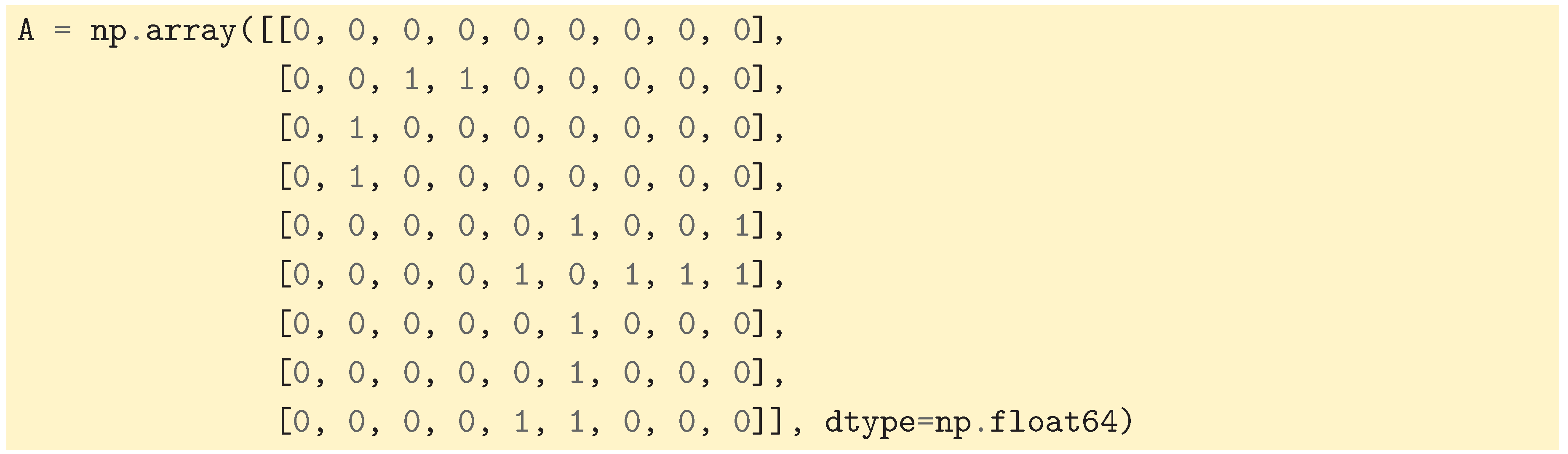
5.5. Multiplicity of the Zero Eigenvalue

We now consider the case where the graph is composed of multiple connected components.

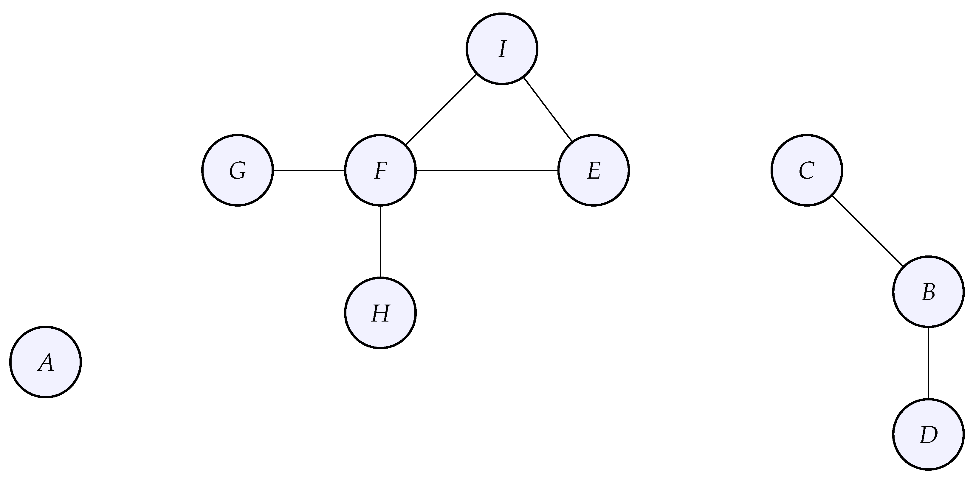
Figure 12. The multiple connected components graph whose adjacency was given above. This graph G has 3 connected components: $G_1=\left\{A\right\}$, $G_2=\{G,F,I,E,H\}$ and $G_3=\{C,B,D\}.$

Figure 12. The multiple connected components graph whose adjacency was given above. This graph G has 3 connected components: $G_1=\left\{A\right\}$, $G_2=\{G,F,I,E,H\}$ and $G_3=\{C,B,D\}.$

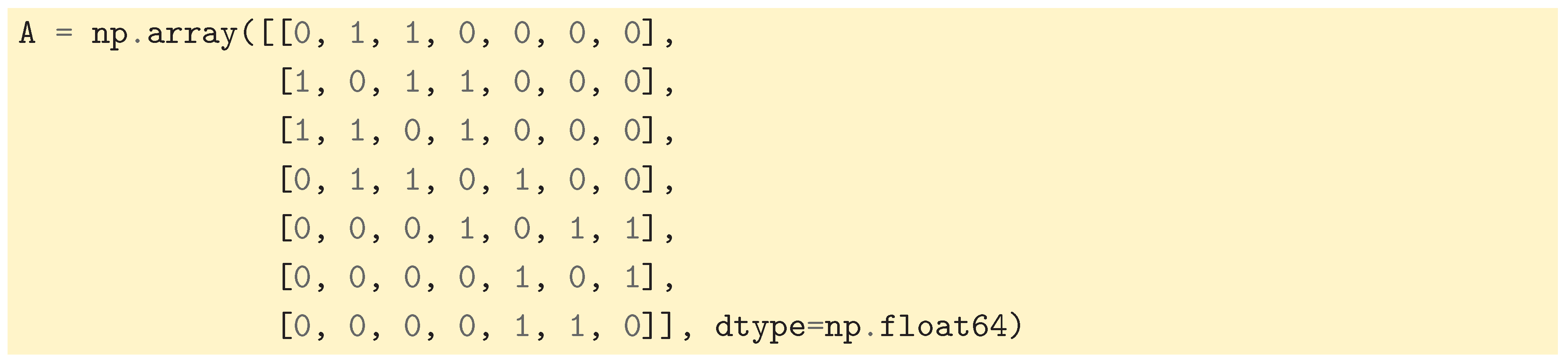
Notice the block structure of the adjacency matrix due to the connected components. This block structure directly transfers to the graph Laplacian which will also have a block structure. The spectrum of the graph Laplacian (its eigenvalues) will also be composed of three different groups of eigenvalues, one for each connected component.

A quick computation that makes use of the definition of the matrix-vector product shows that $L{\mathit{1}}_G=0$ when the graph G has only one connected component, and $L{\mathit{1}}_{G_i}=0$ when the graph G has multiple connected components $G_i$. Here ${\mathit{1}}_G$ denotes the function on G that takes the value one at each node, while ${\mathit{1}}_{G_i}$ denotes the function on G that takes the value one at each node of the connected component $G_i$, zero elsewhere. Indeed,

$${\left(L{\mathit{1}}_G\right)}_i={\left(D{\mathit{1}}_G\right)}_i-{\left(A{\mathit{1}}_G\right)}_i=\sum _j{D}_{i,j}-\sum _j{A}_{i,j}=D_i-\sum _j{A}_{i,j}=0,$$

and similarly for $L{\mathit{1}}_{G_i}$. So, ${\mathit{1}}_G$ is the eigenfunction corresponding to the eigenvalue 0 in the single connected case, and ${\mathit{1}}_{G_i}$ corresponds to the 0 eigenvalue associated to the connected component $G_i$ in the multiple connected case.

Using SciPy like before, we observe that the eigenvalue zero has multiplicity 3, which is exactly the number of connected components of the graph. A mathematical proof of this fact can be found in [6]. Note that when we look at the 3 eigenfunctions related to the zero eigenvalue, we do not recover the 3 functions ${\mathit{1}}_{G_i}$, $i\in \{1,2,3\}$. The reason is that SciPy’s eig method computes a basis of $KerL$ which could be a different basis from $\{{\mathit{1}}_{G_1},{\mathit{1}}_{G_2},{\mathit{1}}_{G_3}\}$.

5.6. The Fiedler Vector

In the previous section we have seen that for a graph G with one connected component, 0 is always the first eigenvalue and ${\mathit{1}}_G$ is the associated eigenfunction. The second eigenvalue is known as the algebraic connectivity, while the associated eigenfunction is called the Fiedler vector. This eigenfunction partitions the graph into two groups: the first group correspond to the nodes with negative coefficients in the Fiedler vector, while the second group corresponds to the nodes with positive coefficients. For example, let’s consider the graph whose adjacency matrix is given by:

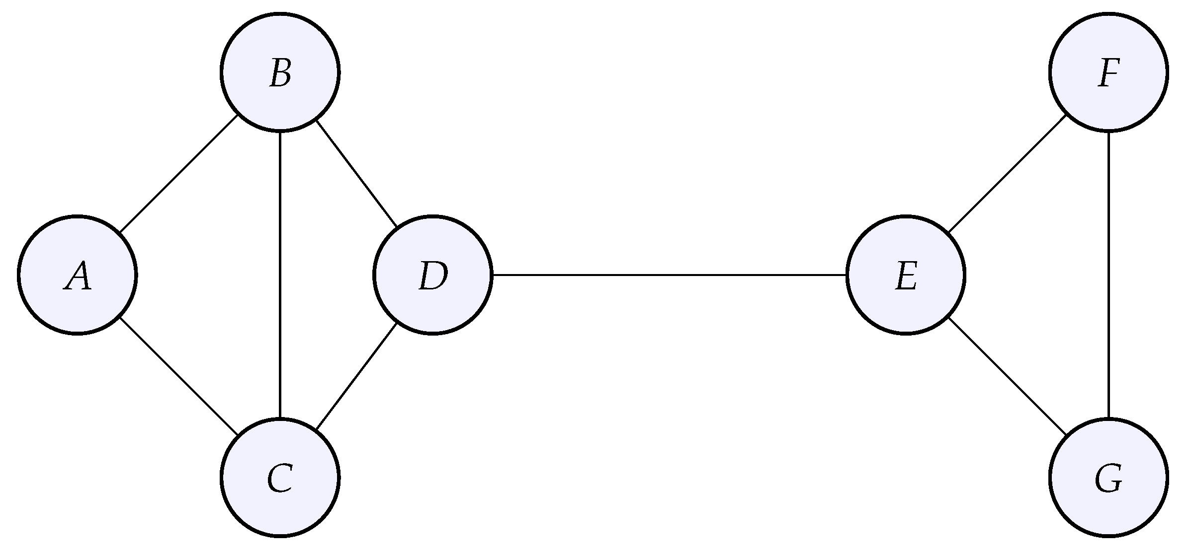
Figure 13. The graph whose adjacency given above.

Figure 13. The graph whose adjacency given above.

Then the Fiedler vector is the second eigenvector of the Laplacian which after computation by ScipPy like before yields:

Therefore, the Fiedler vector separates the graph G into two subgraphs $G_1=\{A,B,C,D\}$ (the first four components are negative) and $G_2=\{E,F,G\}$ (the last three components are positive).

Let us briefly give some intuition into why it is working. The eigenfunction ${\mathit{1}}_G$ (for the eigenvalue 0) represents the whole graph. If we now want to partition the graph into two parts, we would need an eigenfunction that varies as little as possible but is not constant; the nodes over which the variations happen define the groups we have seen above. In other words, we precisely want to find the second eigenfunction (associated to the next eigenvalue after 0, assuming as always that they have been sorted in increasing order). The Rayleigh quotient approach to eigenvalues gives another viewpoint on this second eigenvalue and eigenvector:

$${\lambda }_2=\underset{f\perp {\mathit{1}}_G,\parallel f\parallel =1}{max}{\displaystyle \frac{f^{\mathsf{T}}Lf}{f^{\mathsf{T}}f}}=\underset{f\perp {\mathit{1}}_G,\parallel f\parallel =1}{max}{f}^{\mathsf{T}}Lf,$$

and the minimizer $f_2$ of this optimization problem will be the second eigenfunction. If we imagine the graph as a network of springs with stiffness matrix given by L, then it means we are searching for a state that minimizes its potential energy that is not the trivial state (represented by ${\mathit{1}}_G$). Then from expression (1) it means that nodes that are tightly connected tend to have similar components in $f_2$, while weakly connected groups get different values. It is possible to be more mathematically precise, see [6], where it is proven that searching for the second eigenvalue and eigenvector is equivalent to cutting the graph into two parts.

6. Spectral Clustering

Let us first recall what clustering is about. Clustering is a mathematical procedure to automatically discover and partition data into several groups (the clusters), in an unsupervised fashion (no extra data guides the algorithm). It has multiple applications in Science (for instance, discovering species in a large group of flowers), manufacturing (for instance, to segment the market for a given product into different sizes) and many others. One traditional method to cluster data points that sit in ${\mathbb{R}}^n$ is k-means (see [11]), which does so by iteratively assigning each data point to the nearest cluster centroid and then recalculating the centroids. The primary goal is to minimize the squared distances between each data point and its assigned cluster’s centroid, which results in minimizing the total within-cluster sum of squared errors. This process continues until both the cluster assignments and the centroids no longer change, according to a certain criterion. We would like to do the same with graphs, but there are essentially two issues:

• The first is that a graph is an abstract structure: the nodes are not a priori embedded in any ${\mathbb{R}}^n$ and so we cannot use the k-means algorithm directly. To each node we could assign a point in ${\mathbb{R}}^n$ and then use k-means clustering but such a mapping of a node onto a point would have to reflect the relationships between the nodes, which is not easy to do (this has developed into a whole field of data science known as graph embeddings).
• The second issue comes from the nature of the k-means method itself: it works well with data that is naturally grouped into blobs or, more generally, convex regions, which are linearly separable. When this is not the case, k-means fails. Graphs, once embedded, are usually manifolds, which means that data is not organized into convex, linearly separable regions.

Spectral clustering is a clustering technique specially designed for graphs in order to circumvent the problems mentioned above (see [12] for a modern reference). It uses the eigenvectors of the graph Laplacian to create a meaningful embedding of the nodes, such that, in the embedding space, the data becomes untangled and we can apply k-means. First, recall that when we are searching for eigenvalues and eigenvectors of a linear transformation (matrix), we obtain the principal directions of the transformation (the eigenvectors) together with their magnitude (the eigenvalues). When transferring this point of view to the case of the graph Laplacian, the eigenvectors correspond to the directions in which functions on the graph will have important deviations from the mean, while the eigenvalues correspond to the magnitude of these deviations. If we conceptualize the clusters as being groups of similar nodes, then it means that within these regions of the graph, the deviation should be small. Therefore, we are looking at the smallest eigenvalues and the associated eigenfunctions: we have seen in Section 5 that the eigenfunction associated with the first eigenvalue is representing the whole connected component, and the eigenfunction associated with the second eigenvalue, the Fiedler vector, partitions the graph into two groups of nodes. Suppose we know the graph can be grouped into k clusters or that we want it to be grouped into k clusters. The method of spectral clustering consists of computing the first k eigenvalues (in ascending order) of the graph Laplacian together with the associated k eigenfunctions $f_1,\dots ,f_k\in {\mathbb{R}}^N$ (recall that N is the number of nodes in the graph). Using the analogy between the graph and a network of springs, we are looking at the smallest vibration frequencies and the associated vibration modes. If we now stack the eigenfunction into a matrix $U=[f_1|\dots |f_k]\in {\mathbb{R}}^{N\times k}$, each row of U corresponds to the embedding of the corresponding node in ${\mathbb{R}}^k$. This embedding is sometimes known as the spectral embedding. In the newly formed embedding space ${\mathbb{R}}^k$, euclidean distances correspond to graph distances and simplifying the exposition, the issues we mentioned earlier disappear so that k-means can be applied (to understand mathematically why, see [6]).

Let us wrap up the spectral clustering method with an example. In the following, we will use the normalized Laplacian, as we have seen in Section 4.5. It has the effect of normalizing those nodes that have a large degree.. Without normalization, nodes that are more connected overall can distort the geometry of the embedding space and obscure the true cluster structure to some extent.

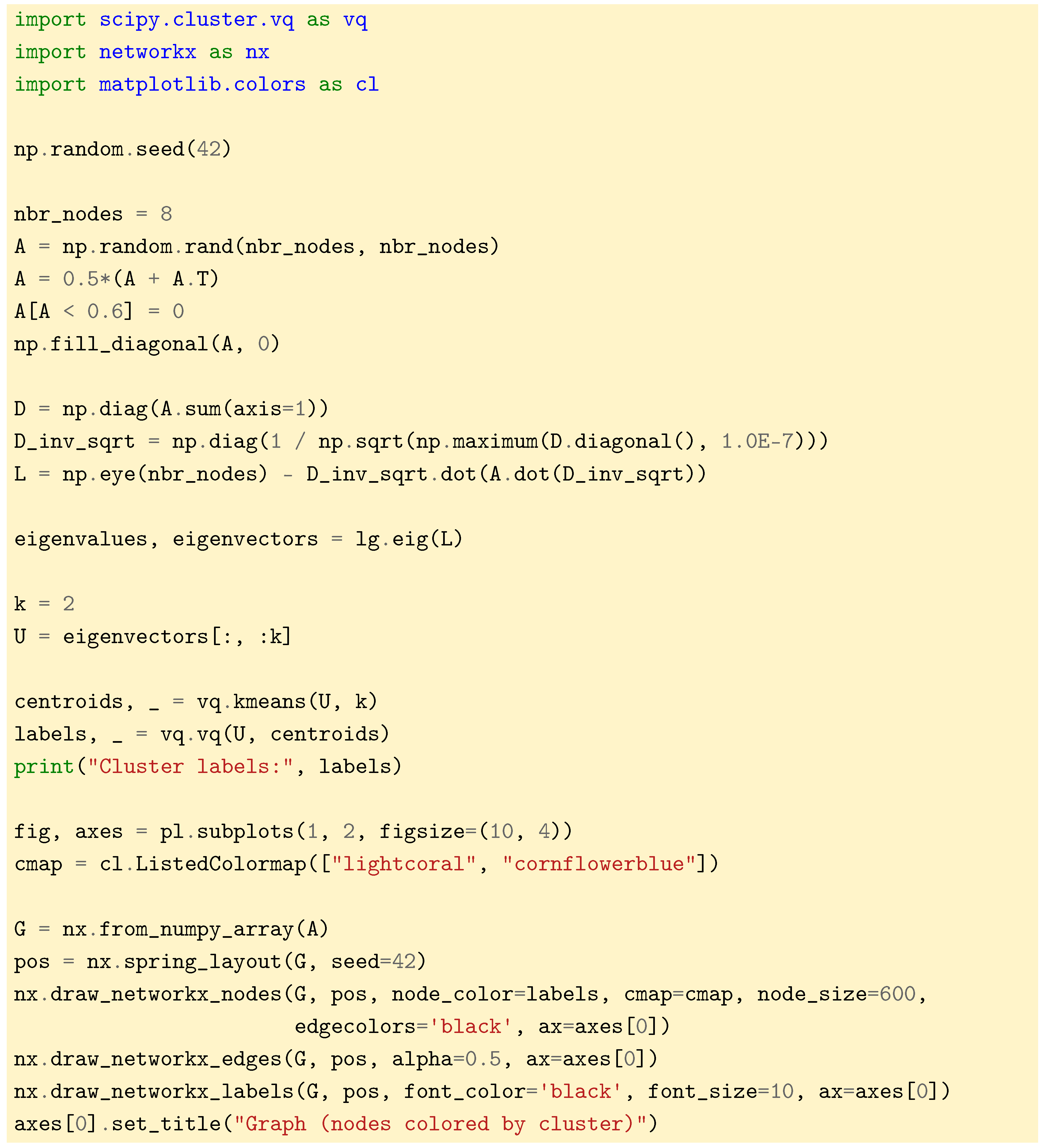
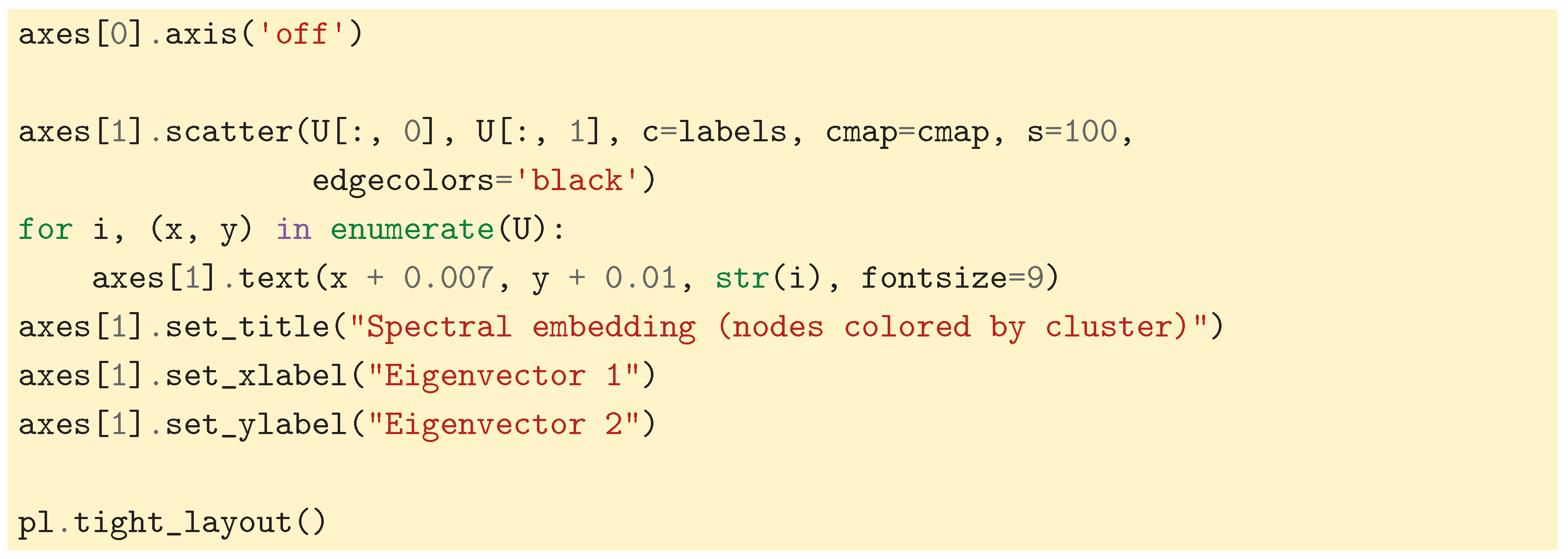
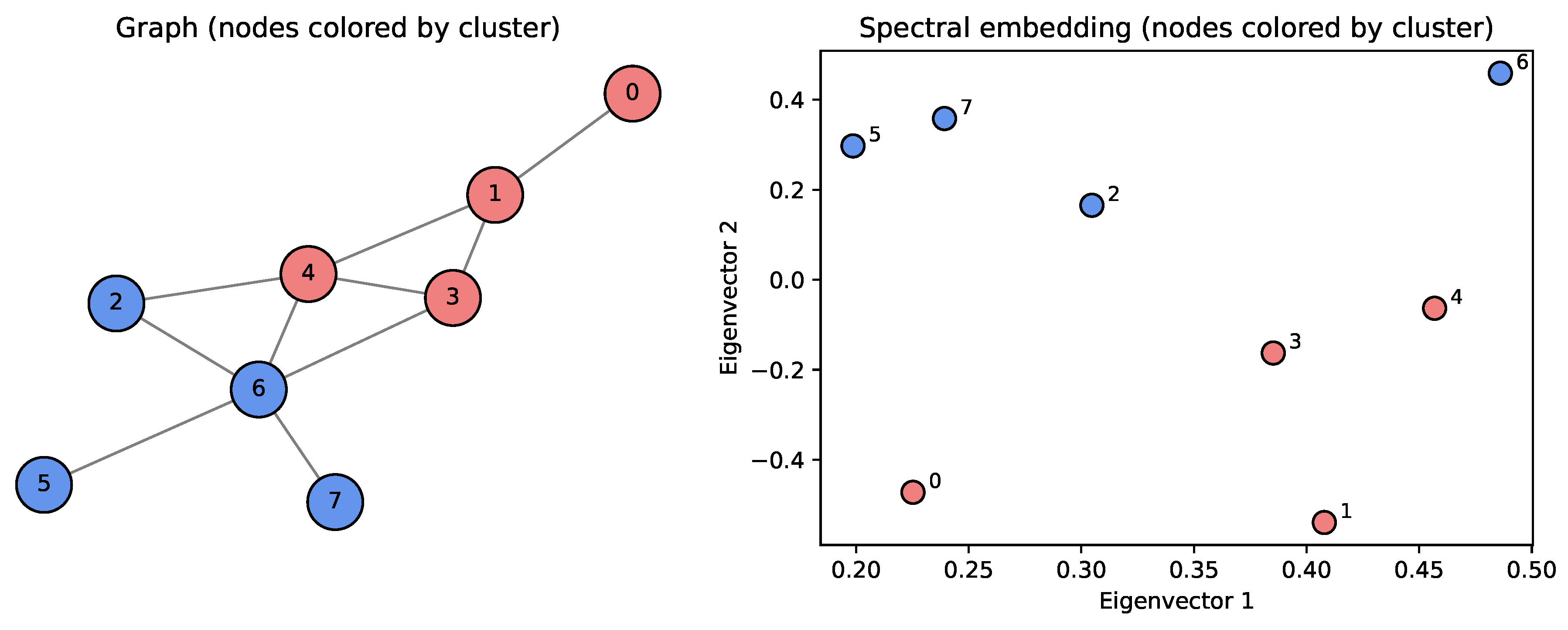
The code above generates a random graph, computes the normalized Laplacian along with its eigenvectors that are used to create the spectral embedding. Then k-means (with $k=2$) is applied by calling the appropriate routine from SciPy. In practice, the number of clusters k is determined by looking at a plot of the eigenvalues: if we spot a large gap (called the spectral gap) between two consecutive eigenvalues ${\lambda }_k$ and ${\lambda }_{k+1}$, then k is usually a good estimate for the number of clusters in the data. We then draw the graph where the nodes are colored according to the cluster they belong to, and we also draw a plot showing all nodes in the spectral embedding space. We can notice that the nodes are clearly linearly separable after using the spectral embedding.

Figure 14. Viewing the clusters and the nodes in the spectral embedding space.

Figure 14. Viewing the clusters and the nodes in the spectral embedding space.

7. The Probabilistic Point of View

In this section, we further our exploration by giving another point of view on clustering which comes from Probability Theory. Given a graph and its adjacency matrix A, the matrix $P=D^{-1}A$ is the transition matrix for a random walk on the graph: if $x^{\mathsf{T}}\in {\mathbb{R}}^N$ (where N is still the number of nodes of the graph) denotes the probability distribution of the random walk at some time, then $xP$ is the distribution of the random walk at the next time, which essentially gives the probabilities that adjacent nodes can be reached by the random walk.

The graph Laplacian is the infinitesimal generator of the random walk, which essentially gives the expected infinitesimal change of a function on the state space of the walk after an infinitesimal amount of time elapsed. In the case of a discrete Markov chain ${\left(X_n\right)}_{n\ge 0}$, the definition simplifies because we only have discrete steps in time. Given a function $f\in {\mathbb{R}}^N$ on the graph, the infinitesimal generator $G:{\mathbb{R}}^N\to {\mathbb{R}}^N$ of the random walk is the linear operator defined by:

$${\left(Gf\right)}_i=error\left[f\left(X_{n+1}^i\right)\right]-f_i,$$

where $X_{n+1}^i$ denotes the node at which the random walk is located at time $n+1$, knowing that it passed through the i-th node at time n, and $f\left(X_{n+1}^i\right)$ denotes the value of f at that new node. Fortunately in our case the infinitesimal generator can be computed easily:

$$\begin{array}{cc}\hfill {\left(Gf\right)}_i& =\sum _{j\in \mathcal{N}\left(i\right)}{P}_{i,j}{f}_j-f_i\hfill \\ \hfill & =\sum _{j\in \mathcal{N}\left(i\right)}{\displaystyle \frac{w_{i,j}}{d_i}}{f}_j-f_i\hfill \\ \hfill & ={\displaystyle \frac{1}{d_i}}\sum _{j\in \mathcal{N}\left(i\right)}{w}_{i,j}(f_j-f_i)\hfill \\ \hfill & ={\left(L_{\mathrm{rw}}f\right)}_i,\hfill \end{array}$$

where $L_{\mathrm{rw}}=D^{-1}L=I-D^{-1}A=I-P$ is the random walk Laplacian as introduced in Section 4.5. From this very relation between the transition matrix and the graph Laplacian, we see that studying eigenvalues and eigenvectors of P is equivalent to study the ones of $L_{\mathrm{rw}}$. For instance, stationary distributions $x^{\mathsf{T}}\in {\mathbb{R}}^N$ of the random walk satisfy $x=xP$, which is equivalent to $L_{\mathrm{rw}}{x}^{\mathsf{T}}=0$. It means that it is possible to compute connected components of the graph from the transition matrix of the random walk.

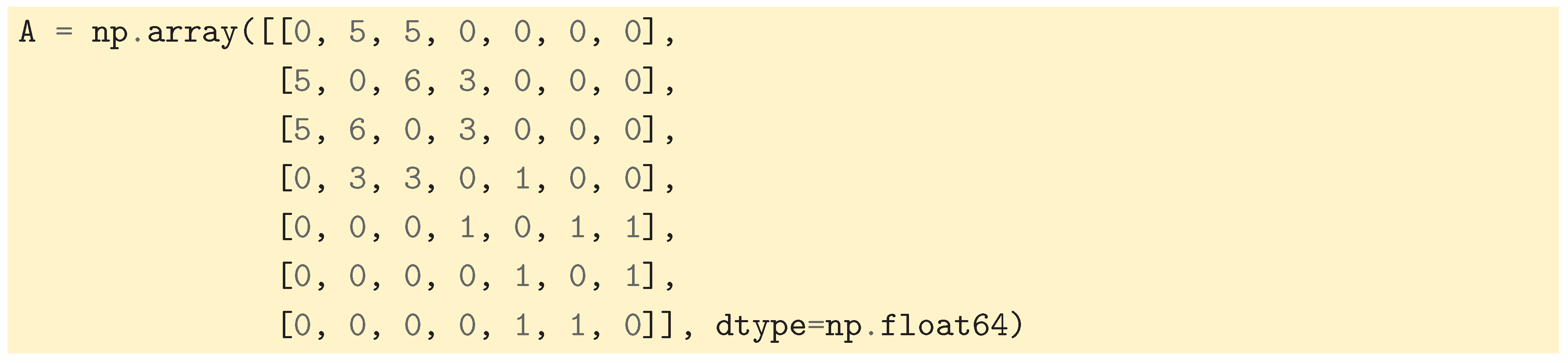
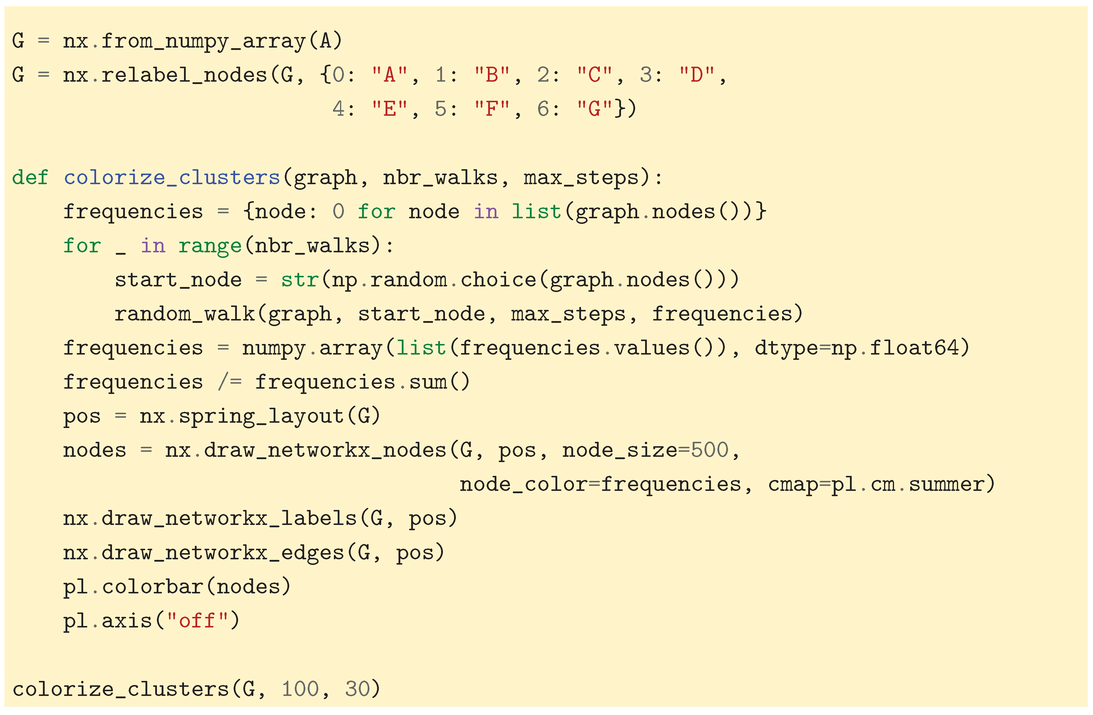
The previous ideas have given rise to a variety of clustering algorithms based on random walks on the graph, either by studying the transition matrix, or by repeatedly sampling the random walk, and observing how the structure of the graph unravels as the walk spends time in clusters (see [13] and [14]). To provide intuition for this important concept, we propose a simulation. This simulation demonstrates how simply recording the visit frequency of the nodes can reveal the underlying cluster structure of the graph. We first define a function that performs (a certain number of steps of) a random walk:

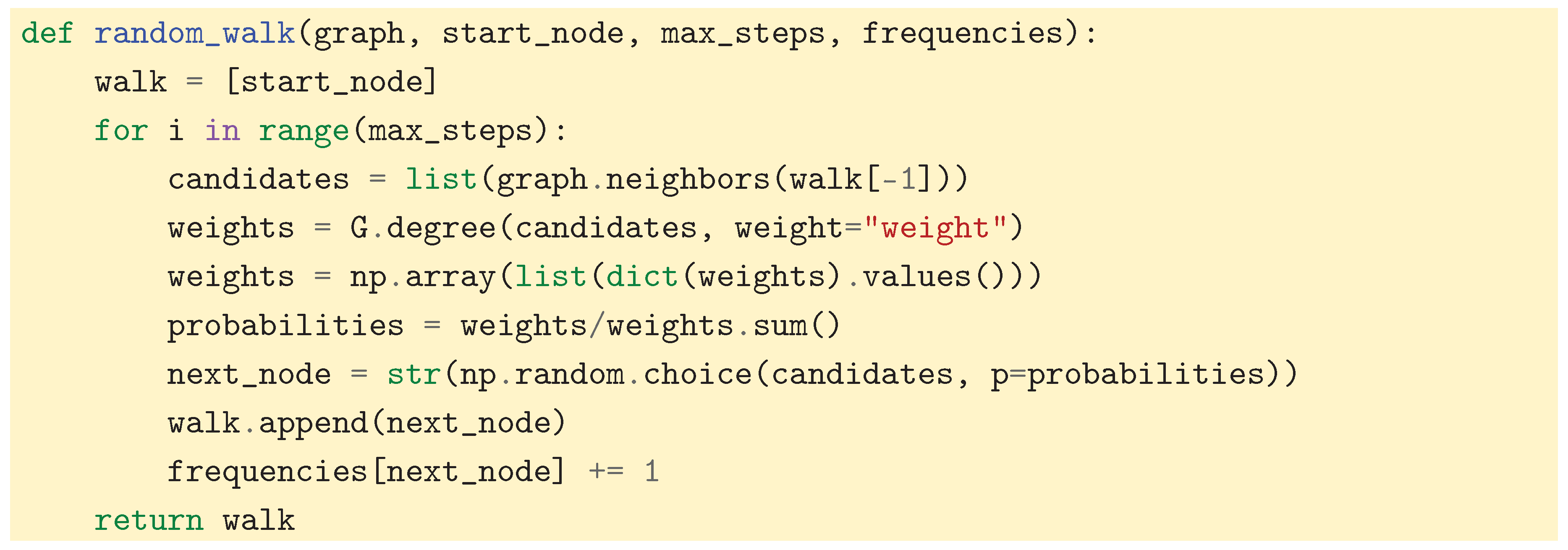
In the simulation, the transition probabilities must be recomputed at each time step. For efficiency, one could instead compute the transition matrix once and for all and use it to improve computational performance. To capture the clusters, we then start multiple random walks at random start nodes and record all the visit frequencies. Note that we use the weighted graph defined in Figure 13 together with the weighted random walk Laplacian to facilitate the demonstration.

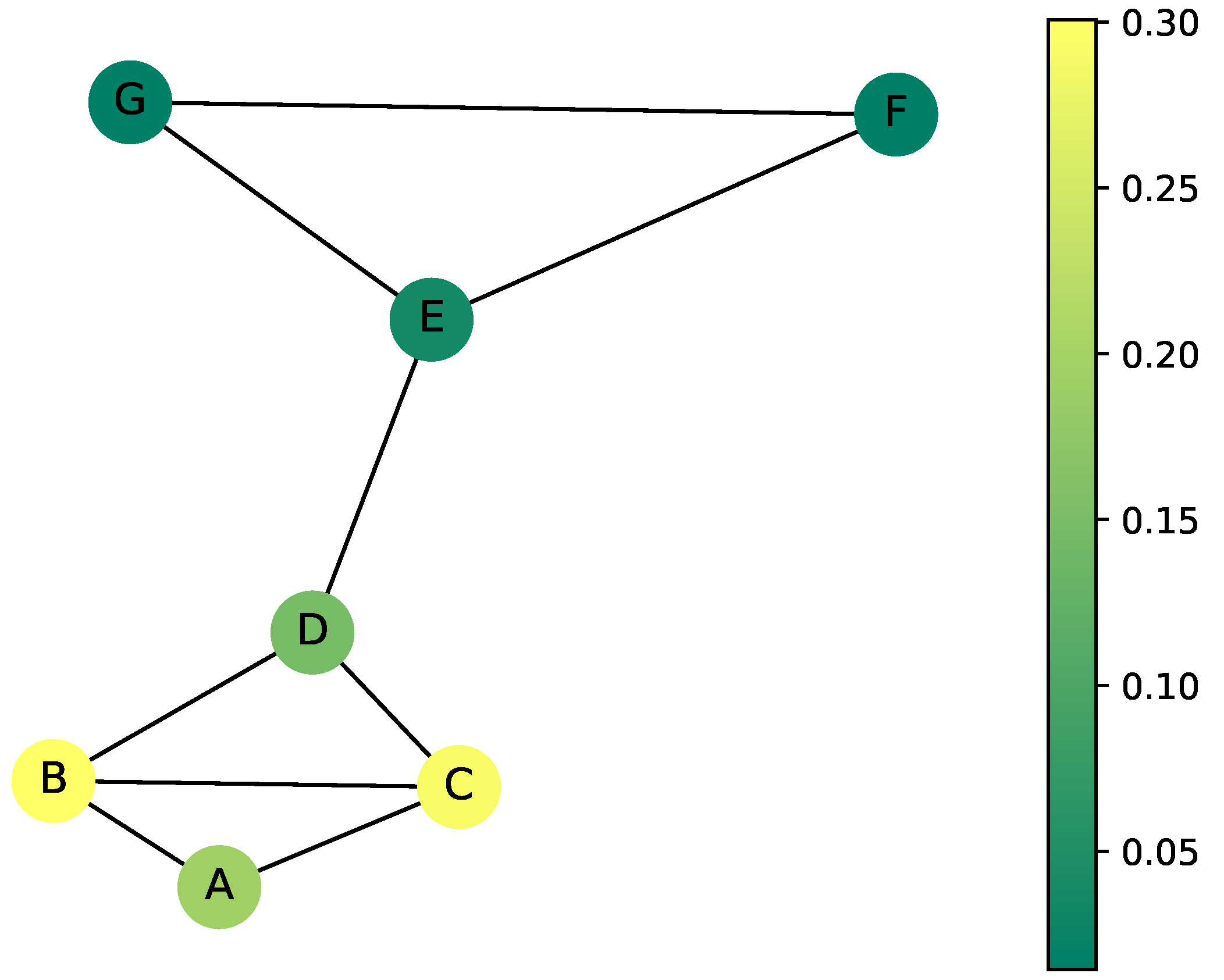
Figure 15. This simulation highlights clusters by recording the visited nodes. The higher the color, the higher the number of times the node was visited. The difference in colors between the groups $\{G,F,E\}$ and $\{B,D,C,A\}$ is the first indicator of where the clusters are.

Figure 15. This simulation highlights clusters by recording the visited nodes. The higher the color, the higher the number of times the node was visited. The difference in colors between the groups $\{G,F,E\}$ and $\{B,D,C,A\}$ is the first indicator of where the clusters are.

Visit frequencies are just the first statistics that come to mind when trying to capture the clusters of the graph. Others are: return probabilities or expected time of return to a certain node, commuting times between two nodes, and also the escape probability from a ball which is related to metastability. Some of these statistics are related to the eigenvalues of the random walk Laplacian. In recent developments, diffusion distances have played an imported role and gave rise to a new method for clustering graphs known as diffusion maps (see [15] and [16]), of which we introduce just the main idea in the following. Starting at a node i and running a random walk on the graph for n steps, we obtain a distribution $P_{i,•}^n$, which indeed is the i-th row of the transition matrix P raised to the n-th power. If nodes i and j belong to the same cluster, then the probability distributions $P_{i,•}^n$ and $P_{j,•}^n$ should be similar, as distributions. The diffusion distance between two nodes i and j is then defined as:

$$D_n{(i,j)}^2=\sum _k{\displaystyle \frac{{(P_{i,k}^n-P_{j,k}^n)}^2}{{\pi }_k}},$$

where $\pi$ denotes the stationary distribution (equilibrium distribution) of the random walk, defined by $\pi =\pi P$ as mentioned previously. Essentially, nodes are close with respect to the diffusion distance if the random walk exhibits similar mixing behavior when starting from them. It is different from the natural distance on the graph, which measures how many steps there are between two nodes. Diffusion distance is global in nature as it measures the similarity with which these two points explore the whole graph. Also, the number of steps n plays an important role: the larger the number of steps is, the more global the cluster structure. Therefore, diffusion maps are also able to discover cluster structures at different scales, see [17]. Also, it turns out that the diffusion distance can be directly computed from the eigenvalues and eigenvectors of $P^n$, or the graph Laplacian alternatively. Readers interested into probabilistic approaches to clustering are invited to look at [18] and [19], Chapter 9].

8. Application to RNA-seq Data

Several active natural science research areas employ graphs. For example, bioinformaticians search for gene regulatory networks by trying to reconstruct the graph of the true relationships between genes. To accomplish that, we can examine the transcriptome in certain conditions of interest, and search for gene modules by spectral clustering.

This section assumes basic knowledge of bioinformatics, such as knowledge of what RNA-seq data is. In the following, we demonstrate the theory discussed in previous sections by analyzing bulk RNA-seq data from [20]. This dataset is composed of several breast cancer cell lines (MCF7, T47D, MDA-MB-231, Hs578T) and a cell line of human foreskin fibroblasts (HFF). All cell cultures were first measured, then treated with chemotherapeutic agents to induce senescence (a dormant, non-proliferative cell state). Lastly, after treatment, repopulating cells (cells that escaped the dormant state) were measured. This resulted in a complex dataset, with several possible conditions concerning both molecular subtype and treatment.

Analyzing such complex data poses unique challenges in interpretation and visualization. For example, RNA-seq data has much larger dimensions than previously presented data in this work, and is also more noisy. Another matter is that regulation is not straightforward. The relationship between two related genes, as detectable in RNA-seq, may or may not be linear. And yet an other issue can be that the signal in RNA-seq data is not deterministic of the underlying regulatory relationship. To illustrate this latter point, let us say that the expression of two genes shows a strong correlation. This can mean that one regulates the other, or, that a third gene regulating both at the same time. While this list of challenges is not exhaustive, it aims to highlight some of the differences between mathematical theory and practical application. With our application example, we aim to underline the importance for both natural scientists to understand complex mathematical methods, and mathematicians to understand practical application. This mutual understanding is necessary for better scientific research.

8.1. Methods

We use bulk RNA-seq data composed of five cell lines (MCF7, T47D, MDA-MB-231, Hs578T, and HFF) and three treatment conditions (control, senescent, and repopulated) [20]. We first preprocess the raw count matrix as described by Bajtai and colleagues [20], then obtain a similarity matrix by computing the pairwise distance correlation between each possible gene pairs. We set the main diagonal to zero, so as to not consider self-relationships. Then, we compute the random-walk normalized graph Laplacian, and its eigendecomposition. We determine the number of gene clusters, k, by taking the elbow of the spectrum, and employ k-means clustering with $k+1$ clusters in the space spanned by the first k eigenvectors aside from the trivial solution corresponding to the zero eigenvalue. We compute $k+1$ clusters to allow for genes that do not belong in any active functional modules to cluster separately. This concludes the spectral clustering step. We then visualize the data and interpret the results, as laid out below.

8.2. Data Visualization and Interpretation

First, we explored the data using Principal Component Analysis (PCA) to obtain a general impression of inherent groups. While data can be clustered after PCA, here, we only employ the technique for visualization. Our paper does not make it a point to thoroughly contrast PCA-based clustering with spectral clustering, but briefly, PCA is designed for data that lie on vector spaces, not manifolds, and therefore often fails to capture non-linear trends; spectral clustering, however, is not constrained by this linearity assumption. In Figure 16 we see roughly three groups split by molecular subtypes. Three of the cell lines, MDA-MB-231, Hs578T, and HFF appear to be more closely related. This is due to their shared biological state: they are mesenchymal types. In contrast, cell lines T47D and MCF7 represent luminal phenotypes. Notably, T47D and MCF7 do not form visibly related clusters despite their shared luminal classification. This is due to a key difference in the mutation status of the P53 gene between the two cell lines. Overall, the five cell lines organize into three main groups, which presents a challenge when the goal is to characterize the cell lines themselves.

Regarding treatment conditions, while there seems to be a difference between control, senescent, and repopulated cells, it is not as marked as the separation between the three main molecular subtypes. All in all, Figure 16 tells us that there are clusters and sub-clusters in our data.

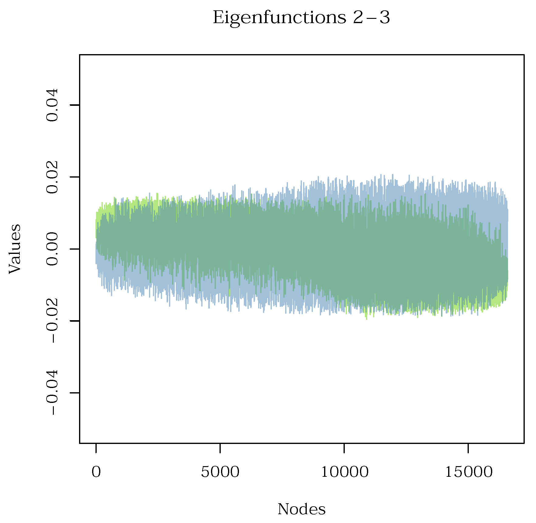
Let us start exploring the potential gene groups that characterize cellular phenotypes. One helpful plot discussed previously is a line-graph of the eigenfunctions. However, this plot is impractical for a large dataset such as ours, as demonstrated by Figure 17.

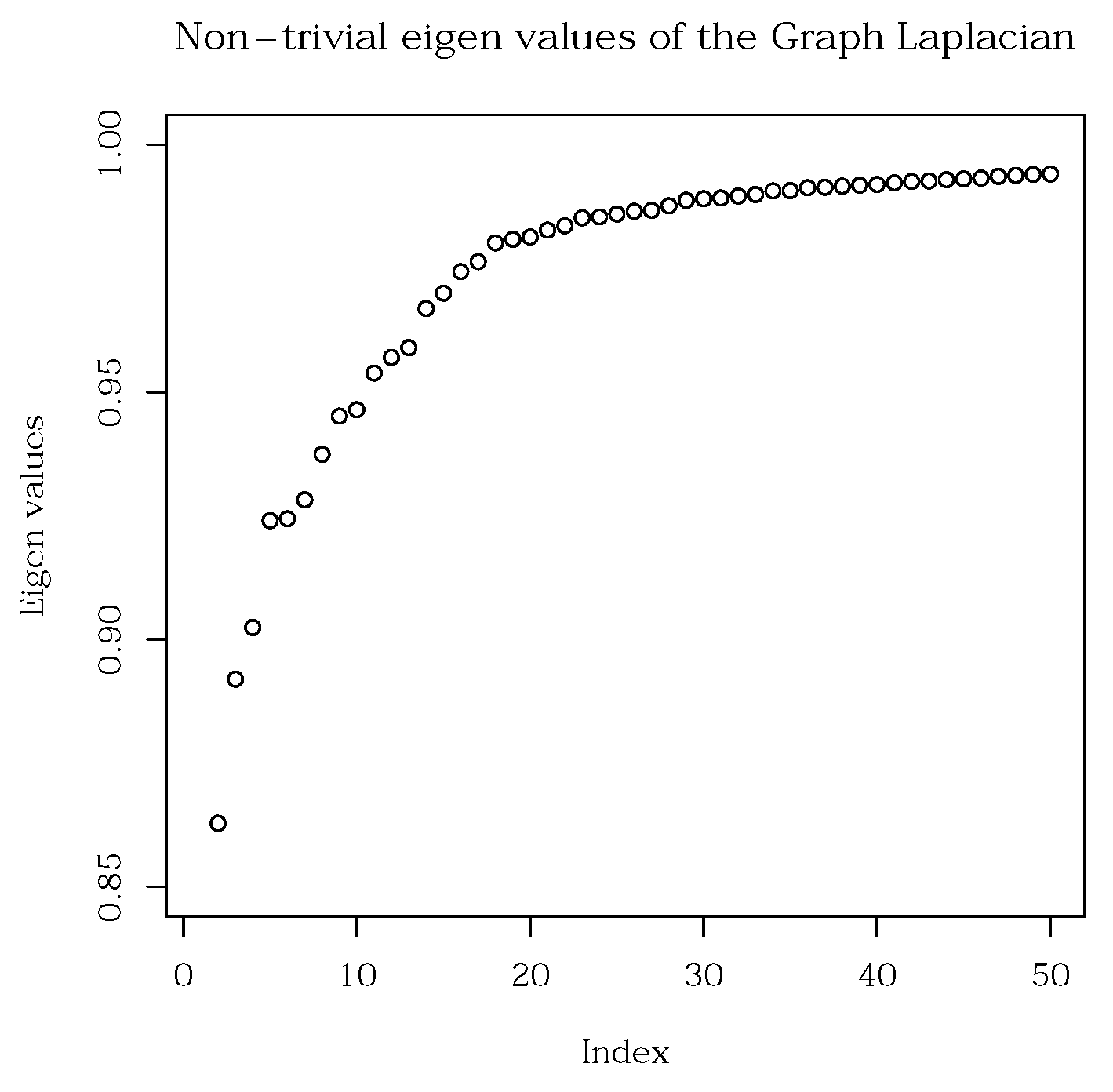
Therefore, we summarize the data by alternative means. Firstly, we need to infer the number of clusters present in the data. To do so, we can use the the spectrum as depicted by Figure 18. We first order the eigenvalues of the graph Laplacian (its spectrum) in an ascending order. We then locate the elbow, which determines the number of clusters, k, inherently present in the data. In our present analysis, we find 17 plausible gene clusters. We note here, that theory tells us to employ the spectral gap for this purpose. However, in real data, the connectivity of the graph is increased compared to concise, small examples. This causes the spectrum to be smooth, and the spectral gap no longer be pronounced enough to be easily located.

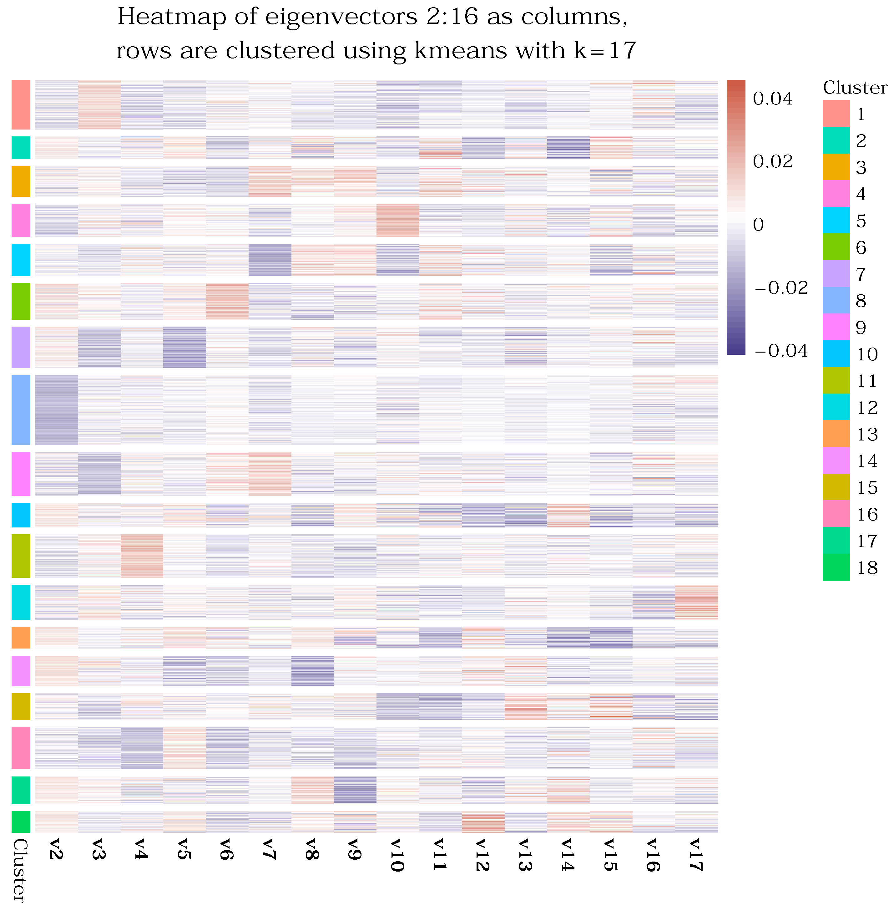
We then employ k-means clustering with $k+1=18$ clusters (to account for a cluster of genes that are not related to the cell conditions, such as house-keeping genes) on the eigenspace spanned by eigenvectors 2 through 17. The results can be neatly visualized using a heatmap, as shown in Figure 19. This heatmap depicts eigenvectors as columns, and maps their components to a color scale, effectively visualizing the eigenvectors of a large dataset. This format allows for easy and quick comprehension of the same information that would be obscured by multiple, superimposed line-graphs as in Figure 17. An added benefit is that the clusters can easily be marked to enrich the plot with even more information. The intensity of the color hue within a cluster directly indicates the strength of that cluster’s association with the corresponding eigenvector.

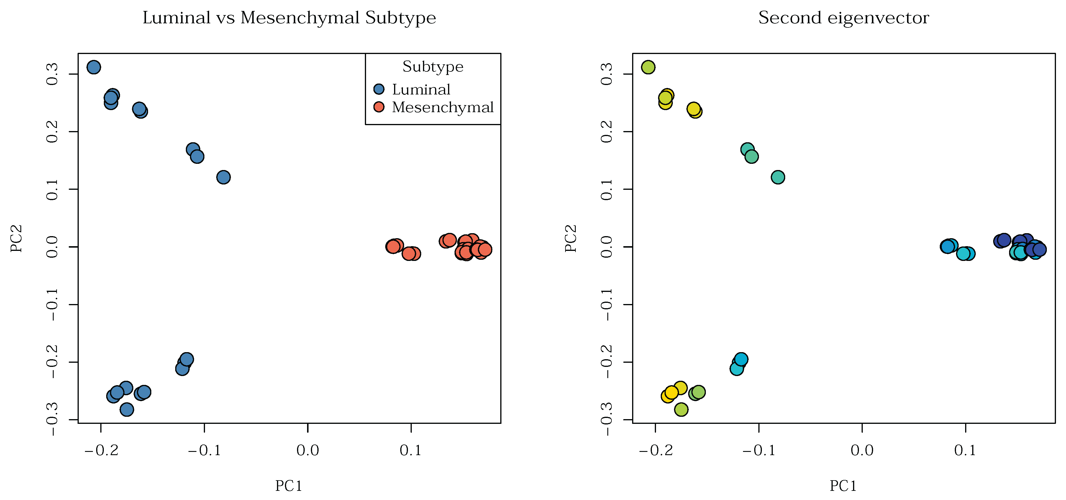
After obtaining gene clusters, usually referred to as gene modules in bioinformatics, we perform enrichment analysis using ToppGene [21]. We discuss results for cluster 8. This cluster, based on Figure 19, could be largely determined by the second eigenvector, $v_2$. Table 1 displays a relevant subset of the enrichment results, the most significant enrichment in coexpressed sets. These sets mark differences between luminal and mesenchymal cells. Based on this, and knowing, that the second eigenvector $v_2$ is associated with this gene group, $v_2$ should logically more-or-less mark luminal and mesenchymal celltypes.

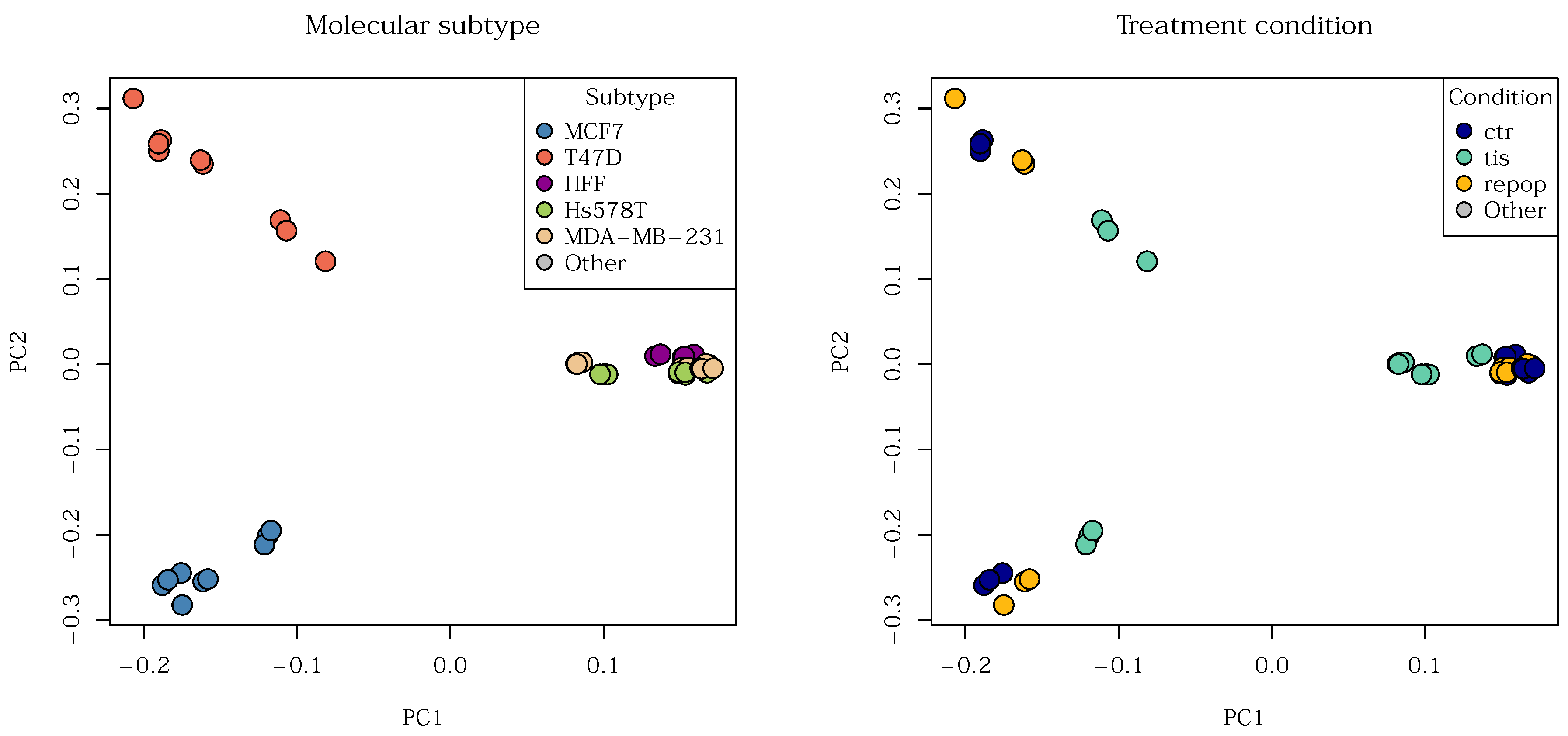
The problem is that $v_2$ is defined in the gene dimension, not the sample dimension. We can mitigate this through transforming the counts by the eigenfunction, meaning, through multiplying the transpose of the count matrix by the second eigenvector of the Laplacian. The resulting vector’s length matches the number of samples, and its components are linear combinations of gene expression. This vector can be used to create a color gradient for the samples, which we can overlay onto our PCA scatterplot. Figure 20 displays the luminal versus mesenchymal subtypes (left), as well as the gradient obtained from the second eigenvector (right): he two visualizations indeed align.

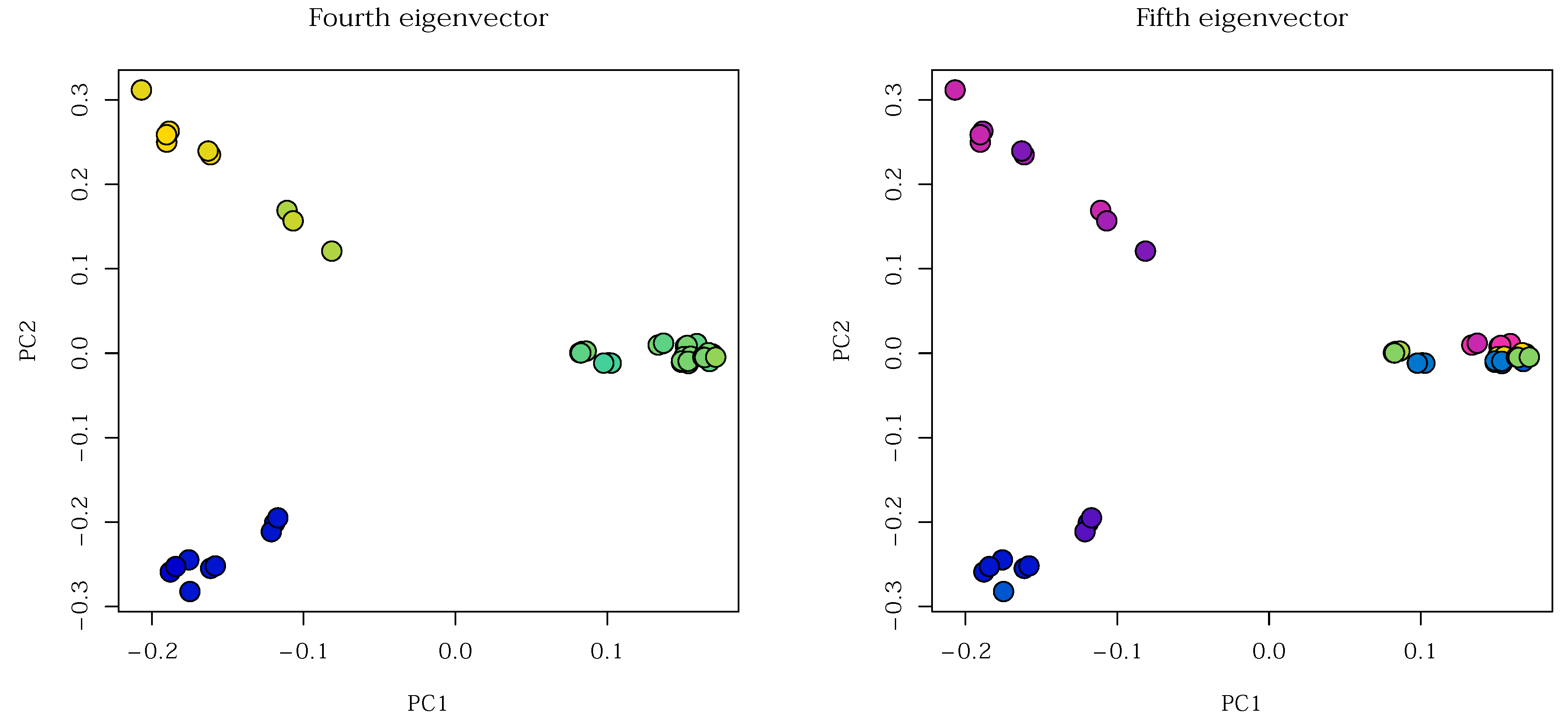
Other eigenfunctions reflect other structures in the data, and can be more granular. For example, the fourth eigenvector appears to differentiate the three main molecular subtypes, while the fifth eigenvector the five cell lines (Figure 21). This demonstrates the ability of spectral clustering to pick up on structures at different scales, and indicates its advantage over linear methods like PCA. Specifically, performing k-means on the first two principal components would likely yield three sensible clusters, but would not identify the cell types. Furthermore, k-means on the first two principal components would likely struggle to differentiate luminal and mesenchymal cells or to resolve differences in treatment conditions.

8.3. Advantages of Spectral Clustering

As the present analysis demonstrates, spectral clustering offers several key advantages:

• It detects both large-scale trends (e.g., luminal and mesenchymal subtypes) and highly nuanced differences (e.g., individual molecular subtypes) in a single run through spectral clustering.
• Particularly in the context of gene-regulatory networks, its modular nature provides flexibility in similarity metric selection and allows for the incorporation of different weights in the adjacency matrix. This flexibility is crucial because gene-to-gene relationships follow various patterns (linear or non-linear), and ideally, we would like to capture most of them.
• Spectral graph theory is an anchor point between three very different fields of mathematics, each approaching the data in its uniquely useful way. The graph interpretation provides a structure for intuitive understanding and organization of gene regulatory relationships. The linear algebraic interpretation enables matrix operations, which are very useful for efficient computation. Finally, the probabilistic point of view offers methods based on random walks, which allow for the modeling of uncertainty and the inference of transitions between biological states.

9. Concluding Remarks

In this article, we explicate spectral graph theory by grounding its core mathematical concepts in intuitive examples. Our paper covers multiple fields, namely, graph theory, linear algebra, and probability theory, demonstrating how spectral graph theory links together these diverse fields of mathematics. We connected the continuous Laplacian operator of calculus to its discrete counterpart on a graph, showing how the resulting eigenvalues and eigenvectors offer a robust framework for revealing hidden structure within complex datasets.

Our practical application to RNA-seq data demonstrated the utility of the technique in real-life data, providing examples of useful visualizations for studying hidden structures within such large and complex datasets. We showed that spectral clustering is capable of identifying both broad trends and nuanced molecular subtypes.

In our concluding remarks, we emphasize that the intersection of sophisticated mathematics and knowledge of natural sciences is necessary for strong and sound scientific research. Therefore, we highly recommend that natural scientists strive for a deeper understanding of mathematics, and mathematicians for a deeper understanding of applications. We hope that our work encourages fruitful interdisciplinary interactions.

References

- Ovall, J.S. The Laplacian and Mean and Extreme Values. The American Mathematical Monthly 2016, 123, 287–291. [Google Scholar] [CrossRef]
- Takane, M.; Bernal-González, S.; Mauro-Moreno, J.; García-López, G.; De-Miguel, F.F. Directed graph theory for the analysis of biological regulatory networks. Frontiers in Applied Mathematics and Statistics 2025, 11. [Google Scholar] [CrossRef]
- Lecca, P.; Lombardi, G.; Latorre, R.; Sorio, C. How the latent geometry of a biological network provides information on its dynamics: the case of the gene network of chronic myeloid leukaemia. Frontiers in Cell and Developmental Biology 2023, 11. [Google Scholar] [CrossRef] [PubMed]
- Luecken, M.D.; Theis, F.J. Current best practices in single-cell RNA-seq analysis: a tutorial. Molecular Systems Biology 2019, 15. [Google Scholar] [CrossRef]
- Chung, F. Spectral Graph Theory; Conference Board of Mathematical Sciences, American Mathematical Society, 1997. [Google Scholar]
- von Luxburg, U. A tutorial on spectral clustering. Stat. Comput. 2007, 17, 395–416. [Google Scholar] [CrossRef]
- Kłopotek, M.A.; Wierzchoń, S.T.; Starosta, B.; Czerski, D.; Borkowski, P. A Method for Handling Negative Similarities in Explainable Graph Spectral Clustering of Text Documents – Extended Version. arXiv 2025, arXiv:cs.CL/2504.12360. [Google Scholar]
- Kunegis, J.; Schmidt, S.; Lommatzsch, A. The Graph Laplacian for Networks with Negatively Weighted Edges; DAI-Labor TU Berlin.
- Demmel, J. Graph Partitioning. University of California at Berkeley CS267 lecture notes.
- Kac, M. Can One Hear the Shape of a Drum? The American Mathematical Monthly 1966, 73, 1–23. [Google Scholar] [PubMed]
- Lloyd, S. Least squares quantization in PCM. IEEE Transactions on Information Theory 1982, 28, 129–137. [Google Scholar] [CrossRef]
- Ng, A.Y.; Jordan, M.I.; Weiss, Y. On spectral clustering: analysis and an algorithm. In Proceedings of the Proceedings of the 15th International Conference on Neural Information Processing Systems: Natural and Synthetic, Cambridge, MA, USA, 2001; NIPS’01, pp. 849–856. [Google Scholar]
- Rüdrich, S. Random Walk Approaches to Clustering Directed Networks. Dissertation, Freie Universität Berlin, 2020. [Google Scholar]
- Avrachenkov, K.; Chamie, M.E.; Neglia, G. Graph clustering based on mixing time of random walks. In Proceedings of the 2014 IEEE International Conference on Communications (ICC), 2014. [Google Scholar] [CrossRef]
- Coifman, R.R.; Lafon, S. Diffusion maps. Applied and Computational Harmonic Analysis 2006, 21, 5–30, Special Issue: Diffusion Maps and Wavelets. [Google Scholar] [CrossRef] [PubMed]
- Coifman, R.R.; Lafon, S.; Lee, A.B.; Maggioni, M.; Nadler, B.; Warner, F.; Zucker, S.W. Geometric diffusions as a tool for harmonic analysis and structure definition of data: Diffusion maps. Proceedings of the National Academy of Sciences 2005, 102, 7426–7431. [Google Scholar] [CrossRef] [PubMed]
- Coifman, R.R.; Lafon, S.; Lee, A.B.; Maggioni, M.; Nadler, B.; Warner, F.; Zucker, S.W. Geometric diffusions as a tool for harmonic analysis and structure definition of data: Multiscale methods. Proceedings of the National Academy of Sciences 2005, 102, 7432–7437. [Google Scholar] [CrossRef] [PubMed]
- Blanchard, P.; Volchenkov, D. Random Walks and Diffusions on Graphs and Databases: An Introduction; Springer Series in Synergetics; Springer Berlin Heidelberg, 2011. [Google Scholar]
- Ghojogh, B. Elements of Dimensionality Reduction and Manifold Learning; Springer: Cham, 2023. [Google Scholar]
- Bajtai, E.; Kiss, C.; Bakos, É.; Langó, T.; Lovrics, A.; Schád, É.; Tisza, V.; Hegedus, K.; Fürjes, P.; Szabó, Z.; et al. Therapy-induced senescence is a transient drug resistance mechanism in breast cancer. Molecular Cancer 2025, 24, 128. [Google Scholar] [CrossRef] [PubMed]
- Chen, J.; Bardes, E.E.; Aronow, B.J.; Jegga, A.G. ToppGene Suite for gene list enrichment analysis and candidate gene prioritization. Nucleic acids research 2009, 37, W305–W311. [Google Scholar] [CrossRef] [PubMed]