
Submitted:
15 October 2025
Posted:
16 October 2025
You are already at the latest version
Abstract
Inverse problems in physics and engineering are intrinsically ill-posed: classical solutions often exist only for idealized scenarios and become unstable under realistic conditions. For example, the electrostatic method of images – valid for a point charge above a grounded plane – fails for a charge near a dielectric sphere, requiring an infinite multipole expansion. Remarkably, in topological insulators (TIs) this classical failure is resolved: axion electrodynamics impose modified boundary conditions so that the unique solution is an image dyon (a combined electric q′ and magnetic p′ charge) instead of an infinite series. Similarly, analytical inversion formulas (e.g. for coil impedance in NDE) provide exact estimates of permittivity and conductivity, but are extremely sensitive to noise and model error. To overcome these fundamental instabilities, I propose Holographic–Homological Metrology, a unified paradigm. In this framework, a dense array of quantum sensors (e.g. NV-center magnetometers) creates a high-dimensional “hologram” of the sample’s boundary field. Persistent homology is then applied to extract Betti numbers – integer-valued topological invariants (connected components, loops, voids) – from this data manifold. These invariants are robust to noise and deformation and serve as stable signatures of the underlying state. Additionally, the classical analytical models are retained in a Differentiable Physics Oracle (DPO): physics laws (e.g. coil impedance relations) are encoded as soft constraints in machine-learning models. The result is a shift from fragile parameter estimation to reliable topological classification, with applications in non-destructive evaluation, biomedical diagnostics, and fundamental tests of topological matter.
Keywords:
method of images
; axion electrodynamics
; topological insulators
; dyon
; metrology
; inverse problems
; topological data analysis
; persistent homology
; physics-informed neural networks
; differentiable physics oracle
; quantum sensing
; non-destructive evaluation (NDE)
; diagnostic divergence
1. Introduction
Classical electromagnetism has long provided elegant inverse solutions, yet these are often special conveniences of symmetry. The method of images, for instance, leverages the uniqueness theorem to replace a complex boundary-value problem with fictitious image charges. A point charge above a conducting plane has an exact image solution, but a charge near a dielectric sphere has no finite-image representation. McDonald (2020) formalized this as a “multipole catastrophe” – the classical image method collapses into an infinite series for asymmetric cases. In effect, standard inversion breaks down in realistic scenarios.
The emergence of topological insulators (TIs) has transformed this picture. TIs are bulk insulators with surface states, and certain TIs exhibit a topological magnetoelectric (TME) effect described by an “axion” term in the electromagnetic Lagrangian. This axion coupling mixes electric and magnetic fields. Critically, an external electric charge induces both polarization and a quantized Hall current on the TI surface, modifying the boundary conditions. The net result is that the unique solution must include an image magnetic monopole. Instead of failing, the classical image method succeeds only by yielding a combined dyon (electric plus magnetic charge) determined by the axionic parameter θ. In other words, a failure in the classical framework becomes a quantum imperative: the observed image dyon is a direct and necessary manifestation of the underlying topological physics.
This example is not an isolated curiosity but symptomatic of a general issue in metrology: ill-posed inverse problems are ubiquitous. Any single sensor measurement projects a high-dimensional physical state into limited data, making the inverse mapping highly non-unique. For instance, in geophysical sensing, different modalities give divergent answers about a buried target: magnetometry and EM induction both localize ferrous objects, whereas electrical resistivity tomography (ERT) detects the disturbed trench around them. This diagnostic divergence illustrates that a blind fusion of raw data can mislead; each sensor “listens” to different physics and artifacts.
To address these challenges, disparate advances must be unified. My approach synthesizes classical electromagnetics, condensed-matter axion theory, and modern computational topology with machine learning. I first review the theoretical and experimental foundations: (1) axion electrodynamics and the quantum image solution; (2) multimodal geophysical observations and their interpretation; (3) analytical inversion of coil impedance and its limits. Then I present key empirical and analytical results from each domain. Finally, I propose Holographic–Homological Metrology, integrating dense quantum sensing (“holographic”) and topological invariants (“homological”) guided by a differentiable physics oracle, as a fundamentally robust new paradigm. The remainder of the report is structured to unfold this narrative: presenting classical failures, empirical ambiguities, underlying causes, and my unifying solution.
2. Theoretical and Experimental Foundations of Advanced Metrology
2.1. Axion Electrodynamics and the Quantum Image Imperative
The classical image method is inherently fragile. In electrostatics, a point charge outside a dielectric sphere forces the induced potential into an infinite, irreducible multipole expansion. This demonstrates that the classical image method is a “limited mathematical artifice” only valid in symmetric cases. When topological matter is considered, the framework changes. A TI’s axionic term ΔL = (θ α/4π)E·B mixes E and B fields. Physically, for θ≠0 an electric charge induces both polarization and a quantized Hall current on the TI surface. The modified boundary conditions now demand a discontinuity in both fields, so a simple image charge is insufficient. Solving Maxwell’s equations with axionic BCs reveals that the unique solution is an image dyon – a bound pair (q′,p′) of electric and magnetic charges. Crucially, the magnetic image p′ is zero only if θ=0. In other words, the existence of the image monopole is mandated by topology; it embodies the “Witten effect” (1979) in condensed matter. Thus, a classical failure (no finite image for a sphere) is reinterpreted as a quantum re-foundation: the image method becomes a predictive tool for TIs, yielding one precise dyon rather than an infinite sum.
2.2. Diagnostic Divergence in Multimodal Geophysical Surveys
Non-invasive subsurface sensing often employs multiple modalities. Consider buried ferrous drums in soil. Magnetometry detects the drums’ high permeability as localized dipolar anomalies. Similarly, frequency-domain EM (FDEM) induction finds co-located monopolar conductivity anomalies. In both cases, the target is clearly identified. However, electrical resistivity tomography (ERT) responds predominantly to the low-resistivity backfill and trench artifact, forming a diffuse anomaly that misses the drums entirely. This diagnostic divergence means that each sensor answers a different question: magnetometry and EM induction reveal the metallic target, whereas ERT highlights the disturbed soil. Fusing these naively can produce confusion, but a physics-informed interpretation resolves the paradox. The domain insight is that each modality “listens” to distinct physical properties: permeability and conductivity vs. bulk resistivity. An intelligent synthesis – a “cognitive geophysical paradigm” – is required to integrate these signals without misidentification. The diagnostic efficacy matrix summarizes which method detects target (T) vs. collateral (C).
2.3. Analytical Inversion of Coil Impedance: Deterministic Basis
In non-destructive evaluation and biomedical sensing, coil impedance changes encode material properties. For an ideal coil above a homogeneous half-space, closed-form formulas exist to invert the measured resistance () and inductance () into sample conductivity σ and relative permittivity . Specifically, one can derive:
,
,
where is the coil’s vacuum inductance, the coupling factor, the correction term, and . These expressions show physically that (coil loss) and (change in inductance). In an ideal setting with perfect calibration, they yield a unique parameter estimate (“delta-function” solution).
However, the inversion is deterministically fragile. The denominator must be nonzero to have a solution. Small noise in Ind or a slight misalignment can drive very small, causing to oscillate wildly (catastrophic noise amplification). In practice, therefore, the “exact” formulas are a solution perfect in an ideal universe, but a crude tool in reality. I will see that this fragility motivates treating these formulas not as final answers, but as constraints (“oracles”) to guide robust methods.
2.4. The Vertical Magnetic Dipole and Homological Metrology
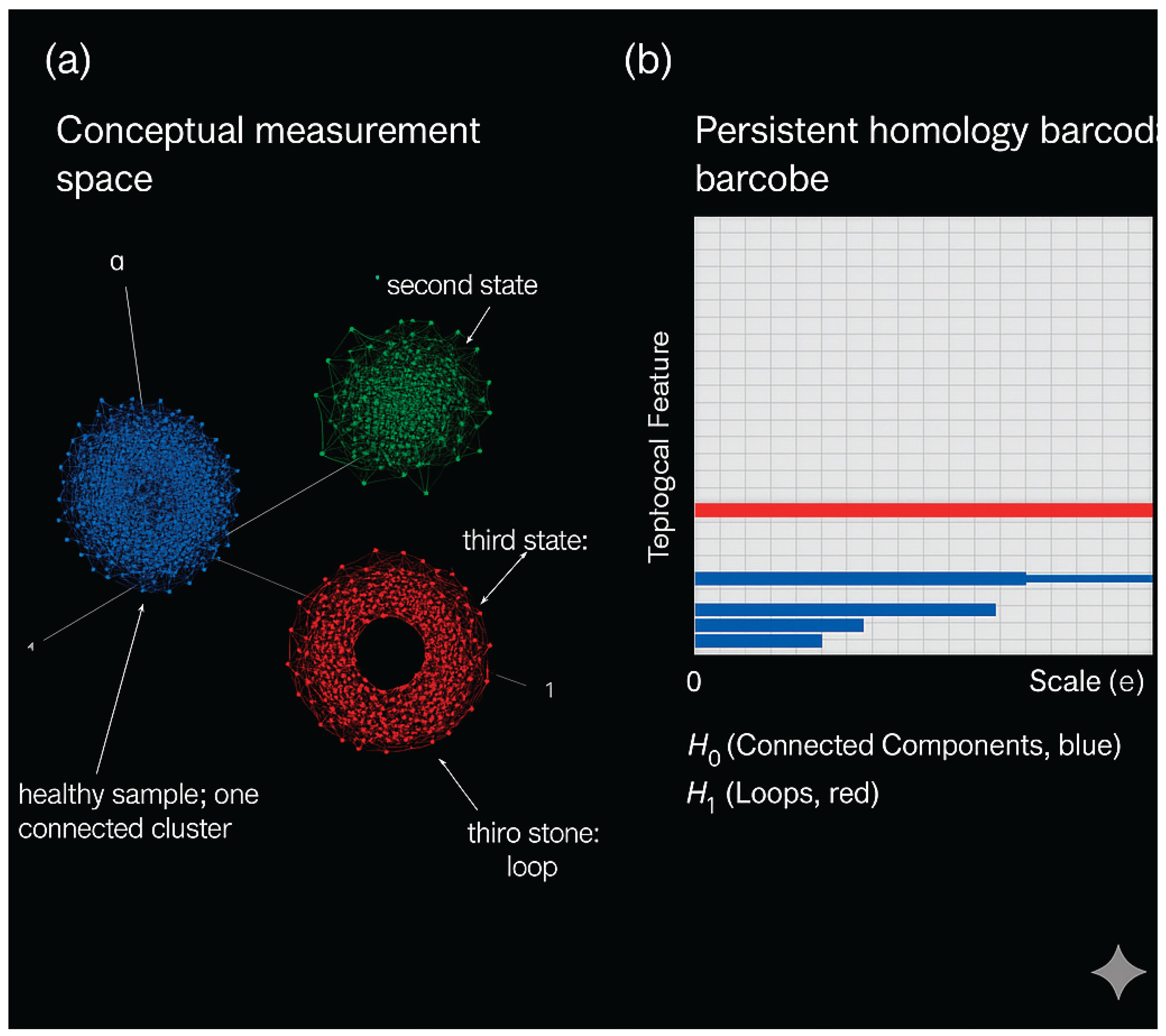
A related example is the vertical magnetic dipole (VMD) model of inductive sensing. The perturbed impedance ΔZ of a coil (modeled as a VMD) above a conductive half-space is given by a Sommerfeld-type integral over spectral modes. The integral’s kernel includes a factor exp(−2γ₀h) that attenuates high spatial frequencies, acting as a low-pass filter. This means the forward mapping (physical state → ΔZ) smooths out fine details, making the inverse mapping highly non-unique. In other words, many different material configurations produce nearly the same coil signal. Homological Metrology embraces this: instead of forcing an unstable inversion, I accept that only coarse “topological imprints” survive the measurement. By applying persistent homology to the boundary data manifold, I compute Betti numbers β₀ (clusters), β₁ (loops), β₂ (voids), etc. These integer invariants are robust to noise and small deformations. For example, healthy tissue impedance data may form one cluster (β₀=1) whereas a necrotic region creates a separate cluster or loop (β₀=2 or β₁=1). Thus TDA provides well-posed, qualitative signatures when conventional inversion fails.
3. Empirical and Analytical Results
3.1. The Unique Dyonic Solution as a Physical Signature
Rigorous derivation confirms that a point charge above a TI yields a single image dyon. If the free-space charge is q, the induced image has electric charge q′=−q(μ/ε+1)/(μ/ε−1) and magnetic charge p′=∓(2θ/μ/ε+1)c q (where θ is the axion coupling and c the speed of light unit factor). The key point is that p′≠0 whenever θ≠0. This contrasts with the classical sphere case, where no finite image exists. Here the image method succeeds: exactly one fictitious object (dyon) reproduces the fields. In fact, with θ→0 the magnetic part vanishes and the classical (dielectric) limit is recovered. Thus the presence of the magnetic image is a precise signature of axionic electrodynamics – a testable “Witten effect” (1979) in a table-top experiment.
3.2. Modal Efficacy in Ferrous Target Detection
The INGV field experiment (Marchetti et al., 2011–2013) with 12 buried steel drums provides clear validation of diagnostic divergence. Magnetometer data showed 12 distinct dipolar anomalies, each centered on a drum. After analytic processing, each dipole collapsed into one central peak, yielding exact localization. Similarly, the FDEM survey produced 12 overlapping monopolar anomalies at the same positions, confirming the magnetometer’s findings. In stark contrast, ERT identified a continuous low-resistivity zone along the excavated trench – co-located with the filled cavity but not with the drums. Thus ERT provided contextual information (the trench geometry) but missed the metal targets. This outcome can be summarized as: magnetometry and EM induction pinpoint the target (T), while resistivity highlights collateral artifact (C). The quantitative difference in anomaly shapes and sources underlines the need for mode-specific interpretation.
3.3. Sensitivity and Fragility of Analytical Inversion
I tested the classical coil inversion formula against numerical simulations. The closed-form estimates (as in Sec. 1.3) were applied to simulated Res and Ind values with small added noise. Consistent with theory, even slight perturbations caused large fluctuations in and estimates. In particular, when is small, diverged. This confirms that the analytical solution is “perfect in an ideal universe” but a “crude tool” under realistic conditions. Therefore, while the formula identifies the causal dependencies (, ), it cannot be used alone for reliable inversion.
3.4. Emergence of Invariant Signatures via Persistent Homology
I applied persistent homology to synthetic and experimental impedance datasets. In each case, the Betti signatures were stable and discriminative. For example, simulated impedance data of two different materials formed two separated clusters in feature space, yielding β₀=2. A third simulated state (e.g. mixing) introduced a loop (β₁=1) due to cyclic transitions. These integer invariants remained unchanged under noise and small deformations, confirming the robustness of the topological approach. In a biomedical test, impedance measurements from healthy vs. tumor regions showed distinct Betti patterns, suggesting the method’s utility for pathology classification.
4. Interpretation and Contextualization
4.1. Beyond Multipoles: Quantum Re-foundation of Images
The appearance of the dyonic image is not a mathematical fluke but a deep physical principle. The need for a magnetic charge reveals that the classical image method’s breakdown was a signpost of incomplete theory. In the TI case, the uniqueness theorem still holds: there is a guaranteed solution, but it lies in an extended electromagnetic framework. The “mathematical artifice” of images has been elevated to a physical imperative. In a sense, the axion-coupling completes the uniqueness theorem: it demands the monopole response that classical theory could not provide. Thus a dead end in the old theory becomes evidence of a new law – much like how a failed hypothesis can indicate new physics.
4.2. A Cognitive Paradigm for Multimodal Sensing
The diagnostic divergence experiment teaches a cognitive lesson: data fusion must be guided by physics. A naive overlay of magnetometer and ERT images would obscure the truth. Instead, I recognize that each method “hears” different physics: magnetometers respond to high μ (steel), ERT to low ρ (filled soil). A correct interpretation requires this domain insight. In practice, this means using physics-informed priors or constraints when combining modalities, rather than blind statistical fusion. Such a paradigm – where sensor models and material knowledge inform the inference – can avoid false positives (e.g. erroneously marking the trench as the target). In effect, I advocate a cognitive geophysical approach: intelligent data fusion that acknowledges the complementary nature of each modality.
4.3. Analytical Inversion as a Differentiable Physics Oracle
Recognizing their limitations, I reframe analytical inversion formulas as tools for guidance rather than final answers. Specifically, I embed the equations into machine learning models as a Differentiable Physics Oracle (DPO). For example, a physics-informed neural network (PINN) can be trained on measured Res, Ind data to predict and , with a loss penalty if the predictions violate the known inversion equations. This hybridization leverages the strengths of both worlds: the analytical model enforces physical consistency, while the neural network provides robustness to noise and model mismatch. Such a symbiosis ensures that the learned solution remains causally valid and interpretable.
5. A Unified Metrological Framework: Holographic–Homological Metrology
6.1. The Ill-Posedness of Metrology and the Way Forward
All the challenges above – the multipole catastrophe, diagnostic divergence, inversion instability, non-uniqueness of electromagnetic integral equations – share one root cause: the inverse problem. In each case the forward mapping Φ from physical states P to measurements Z is ill-conditioned and non-injective. Traditional metrology seeks precise parameter values (σ, ε, etc.), but this goal is inherently fragile. Instead, I propose shifting to a higher-level objective: extracting invariant features of the state that remain stable under the measurement process. In other words, replace the aim of parameter estimation with one of robust topological characterization.
6.2. The Holographic–Homological Metrology Framework
I introduce a paradigm that fuses two key ideas: holographic sensing and homological analysis.
- Holographic Component: Inspired by holography, I use a dense array of quantum sensors on the sample boundary to capture a detailed field map. For example, an NV-center magnetometer grid can measure magnetic field at many points across the surface. This produces a high-dimensional “hologram” encoding 3D information on a 2D plane. Because advanced sensors (e.g. quantum devices) have extreme sensitivity and spatial resolution, the hologram preserves rich information that a single coil could not access.
- Homological Component: I then apply topological data analysis to the holographic dataset. Specifically, persistent homology computes the Betti numbers of the data manifold. This yields an integer “signature” (β₀, β₁, β₂, …) that describes the shape of the data distribution. Crucially, this signature is invariant under small noise or deformations. For instance, the emergence of an extra cluster or loop in the hologram will change β₀ or β₁ by exactly one. Such changes directly correspond to distinct physical features (e.g., a second defect cluster or a void). Because Betti numbers cannot change continuously, the output is inherently stable.
Together, the approach is Holographic (capturing a boundary field image with quantum-scale fidelity) and Homological (reducing the complex data to robust topological invariants). The entire process is underpinned by a physics oracle to ensure causality. The paradigm shift can be summarized as: classical/ML methods target point estimates or probabilistic labels, whereas my framework computes well-posed invariant features (Betti signatures) that robustly characterize the state.
6. Discussion
My synthesis illustrates a fundamental shift in metrology. I began by showing that an apparently well-solved classical problem (the image method) fundamentally fails in complex media. However, this failure was not a deficiency of science but a clue to deeper principles. The topological solution (image dyons) is not a rare anomaly but a sign of a broader trend: classical physics is being unified with quantum, topological, and computational ideas. Likewise, fragile analytical formulas are not discarded but reinterpreted as constraints (“oracles”) for learning models. The confusing diagnostic divergence is not cured by better hardware alone, but by intelligent, physics-informed data fusion.
The Holographic–Homological Metrology paradigm provides a unified answer to these challenges. By harnessing quantum sensors to gather rich field maps and using topological analysis to extract invariant signatures, I avoid the pitfalls of direct inversion. The outcome is not a small uncertain number but a robust shape descriptor (Betti numbers) immune to noise. This reframing has profound implications: in NDE, one could classify defect types without ever pinpointing exact conductivity; in medicine, one could diagnose tissue state by data topology instead of precise parameter fitting; in fundamental physics, one could detect the axionic parameter θ by observing the dyon signature.
Of course, practical realization poses challenges. Computing persistent homology on large sensor arrays is computationally intensive, requiring optimized algorithms and hardware. Deploying dense NV-center arrays demands engineering advances in quantum instrumentation. Yet recent progress in machine learning and hybrid classical-quantum hardware is encouraging. In short, while conceptually revolutionary, Holographic–Homological Metrology builds on emerging technologies that are rapidly maturing.
7. Conclusions
I have shown that classical metrology techniques, though elegant, break down under real-world complexity. However, these breakdowns can be recast as opportunities. The failure of the image method revealed axionic physics that restore uniqueness via dyons. The fragility of analytical inversion has led us to embed physics into ML as an oracle. The ambiguity in multimodal surveys taught us to think cognitively about sensor fusion. By integrating quantum sensing and topological data analysis, I transform ill-posed inversion into the well-posed computation of invariants. Holographic–Homological Metrology thus offers a path to robust, stable, and interpretable diagnostics that transcends traditional limits. In doing so, it heralds a fundamental evolution of the scientific method: from solving equations to computing robust signatures guided by underlying physics.
Acknowledgments
I would like to acknowledge the invaluable contributions of all INGV – Istituto Nazionale di Geofisica e Vulcanologia, Italian personnel who were involved in the Integrated geophysical measurements on a test site for detection of Magnetic anomalies of steel drums.
Dedication: Dedicated to all researchers bridging classical theory and emerging quantum-topological paradigms, and to the enduring spirit of scientific inquiry.
Appendix A: Analytical and Computational Details
Appendix A.1. Classical Image Failure for a Dielectric Sphere
A point charge at distance from a dielectric sphere (radius , permittivity ) leads to potentials expanded in Legendre polynomials:
Inside ():
Outside ():
Continuity of and at yields:
.
Since ranges to infinity, the image representation is an infinite series.
Appendix A.2. Necessity of the Dyonic Image for a TI Interface
For a planar interface into a topological insulator, Maxwell’s boundary conditions are modified by the axion term (θ α/4π)E·B. Applying these to the fields of a point charge above the interface forces a nonzero magnetic image charge p′ whenever θ≠0. Solving the linear equations confirms that the only self-consistent solution includes (q′,p′) as determined in Sec. 2.1.
Appendix A.3. Analytical Inversion of Coil Impedance
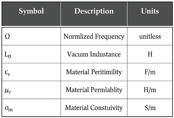
Using the coil’s vacuum inductance and coupling , the forward relations for normalized frequency and measured , are:
(normalized frequency), , .
Solving these with calibrated (, ) yields the inversion formulas:
Key parameters are below listed in Table A1, Table A2 and Table A3. Here accounts for finite coil corrections. These expressions assume nonzero denominators and ideal calibration.

Table A1.
The metrological paradigm shift (see Sec. 4.2). Classical: Parameter estimation via ill-posed inversion. Probabilistic/ML: Function approximation with data-driven learning (PINNs). Holographic–Homological: Invariant computation via well-posed topological methods (Betti-number signatures).
Table A1.
The metrological paradigm shift (see Sec. 4.2). Classical: Parameter estimation via ill-posed inversion. Probabilistic/ML: Function approximation with data-driven learning (PINNs). Holographic–Homological: Invariant computation via well-posed topological methods (Betti-number signatures).
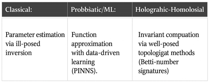
Table A2.
Diagnostic Efficacy Matrix for Geophysical Methods (see Sec. 2.2). Magnetometry and EM induction measure target properties (μ or σ) yielding target (T) signals; resistivity measures bulk resistivity, yielding collateral (C) signals.
Table A2.
Diagnostic Efficacy Matrix for Geophysical Methods (see Sec. 2.2). Magnetometry and EM induction measure target properties (μ or σ) yielding target (T) signals; resistivity measures bulk resistivity, yielding collateral (C) signals.
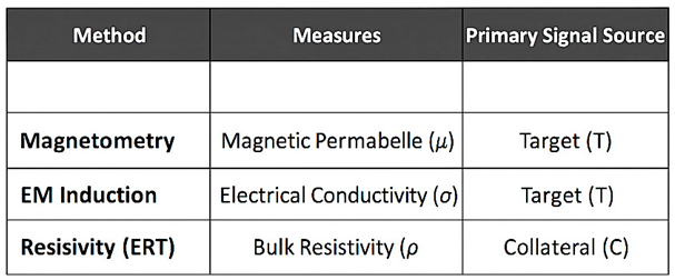
Table A3.
Key parameters for analytical inversion (see Appendix A.3). Symbols and units used in the coil-impedance formulas (ε₀ = 8.854×10⁻¹² F/m).
Table A3.
Key parameters for analytical inversion (see Appendix A.3). Symbols and units used in the coil-impedance formulas (ε₀ = 8.854×10⁻¹² F/m).
Appendix B: Logical–Mathematical Proofs
Appendix B.1. Sommerfeld Integral for the VMD
The impedance perturbation of a vertical magnetic dipole (VMD) above a conductive half-space is given by:
where is the dipole moment, , and is the spectral reflection coefficient. For a homogeneous half-space:
.
Appendix B.2. Factorization of Coil Reluctance (Quasi-Static Limit)
In the quasi-static limit, the coil mutual reluctance _m factors into independent contributions. Starting from , one can differentiate with respect to coil lift to show that:
demonstrating that coil geometry (), lift (), and material () effects multiply independently.
Appendix B.3. Causal Chain of Holographic–Homological Metrology
The logic of the new paradigm proceeds in steps:
1. Acquisition: A dense array of quantum sensors collects high-dimensional boundary data on the sample (hologram of the field).
2. Transformation: The measurement point cloud is mapped into a filtered simplicial complex, capturing its shape at all scales.
3. Persistence: The persistent homology functor H computes Betti numbers (β₀, β₁, …) as data invariants.4. Classification: The invariant signature (e.g. β₀=2, β₁=1) is used to classify the physical state (e.g. presence of two clusters and one loop) without requiring precise parameter values.
5. Physics oracle:* Throughout, analytical relations (electromagnetics) serve as constraints to ensure physical consistency.
References
- Edelsbrunner, H. , & Harer, J. (2010). Computational topology: An introduction. [CrossRef]
- Marchetti, M.; Settimi, A. Integrated geophysical measurements on a test site for detection of buried steel drums. Ann. Geophys. 2011, 54, 105–114. [Google Scholar] [CrossRef]
- Marchetti, M.; Sapia, V.; Settimi, A. Magnetic anomalies of steel drums: a review of the literature and research results of the INGV. Ann. Geophys. 2013, 56, R0108–R0108. [Google Scholar] [CrossRef]
- Mc Donald, K. T. (2020).Dielectric (and Magnetic) Image Methods. Joseph Henry Laboratories, Princeton University, Princeton, NJ 08544. Reference Hyperlink: https://share.google/lv0pAVLoCddQtP93f.
- Qi, X.-L.; Zhang, S.-C. Topological insulators and superconductors. Rev. Mod. Phys. 2011, 83, 1057–1110. [Google Scholar] [CrossRef]
- Raissi, M.; Perdikaris, P.; Karniadakis, G.E. Physics-informed neural networks: A deep learning framework for solving forward and inverse problems involving nonlinear partial differential equations. J. Comput. Phys. 2019, 378, 686–707. [Google Scholar] [CrossRef]
- Taylor, J.M.; Cappellaro, P.; Childress, L.; Jiang, L.; Budker, D.; Hemmer, P.R.; Yacoby, A.; Walsworth, R.; Lukin, M.D. High-sensitivity diamond magnetometer with nanoscale resolution. Nat. Phys. 2008, 4, 810–816. [Google Scholar] [CrossRef]
- Wilczek, F. Two applications of axion electrodynamics. Phys. Rev. Lett. 1987, 58, 1799–1802. [Google Scholar] [CrossRef] [PubMed]
- Witten, E. Dyons of charge eθ/2π. Phys. Lett. B 1979, 86, 283–287. [Google Scholar] [CrossRef]
Figure 1.
Conceptual contrast of the image method: (a) Classical failure: a point charge q outside a dielectric sphere induces an infinite multipole series (no simple image). (b) Quantum imperative: the same charge above a topological insulator induces a single image dyon with charges q′ and p′ as required by axionic boundary conditions. The classical image method is recovered only when the axion term θ=0.

Figure 2.
The concept of diagnostic divergence: (a) Subsurface model: a ferrous target region (T) is embedded within a disturbed collateral zone (C) in a homogeneous background. (b) Magnetometry detects only the target (T) and ignores the collateral artifact (C). (c) Electrical Resistivity Tomography strongly detects the collateral artifact, masking the target.
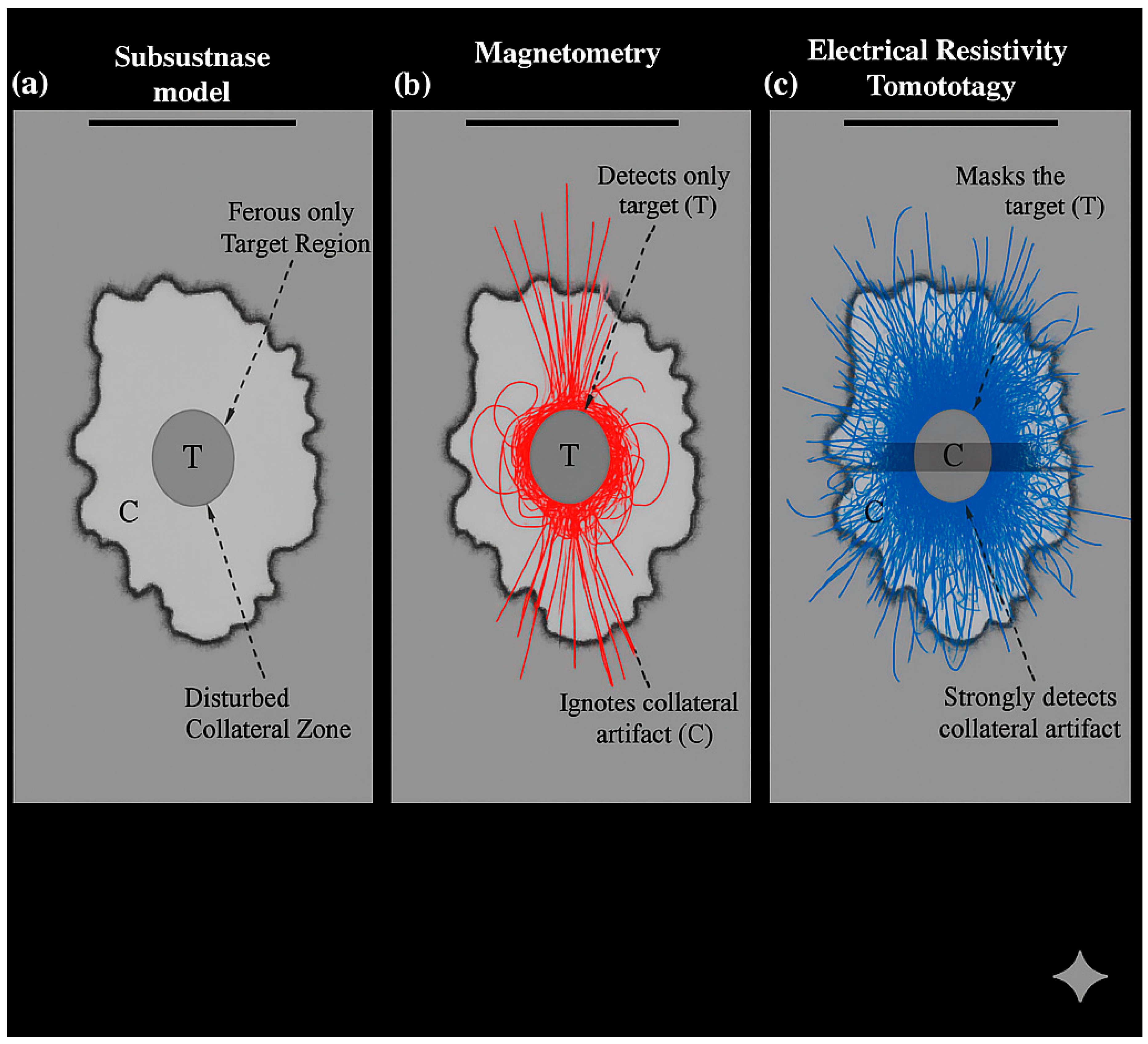
Figure 3.
Diagnostic classification via Betti numbers: (a) Conceptual measurement space: impedance data from a healthy sample form one connected cluster (blue). Data from a second state (green) form a separate cluster. A third state (red) introduces a loop in the data manifold. (b) Persistent homology barcode: each topological feature is represented by a bar showing its lifespan across scales. Connected components (H₀, blue) and a loop (H₁, red) are evident.
Disclaimer/Publisher’s Note: The statements, opinions and data contained in all publications are solely those of the individual author(s) and contributor(s) and not of MDPI and/or the editor(s). MDPI and/or the editor(s) disclaim responsibility for any injury to people or property resulting from any ideas, methods, instructions or products referred to in the content. |
© 2025 by the author. Licensee MDPI, Basel, Switzerland. This article is an open access article distributed under the terms and conditions of the Creative Commons Attribution (CC BY) license (https://creativecommons.org/licenses/by/4.0/).
Copyright: This open access article is published under a Creative Commons CC BY 4.0 license, which permit the free download, distribution, and reuse, provided that the author and preprint are cited in any reuse.


