
Submitted:
07 October 2025
Posted:
08 October 2025
You are already at the latest version
Abstract
Hydraulic conductivity estimation in fractured and clay-rich sedimentary rocks is often challenged by geological heterogeneity and disturbances from drilling operations. This study investigates the applicability of borehole geophysical logging, focusing on spontaneous potential (SP) and single-point resistance (SPR), to establish reliable correlations with hydraulic conductivity in sedimentary formations of Taiwan’s mountainous regions. Conventional approaches based on Archie’s law and formation factors were found to be unreliable due to inaccuracies in pore-water resistivity caused by drilling mud contamination and lithologic complexity. To overcome these issues, a two-stage SP-based screening method was developed to refine datasets by differentiating lithologic intervals and filtering heterogeneous or noise-affected samples. Regression models derived from these screened datasets demonstrated that SPR exhibited the strongest predictive performance, while SP filtering significantly enhanced correlation accuracy. Among the developed models, one provided practical predictions with broader coverage, whereas the more refined model achieved higher precision with fewer data points. The results highlight the advantages of integrating SP screening with resistivity logging to create a cost-effective and systematic approach for estimating hydraulic conductivity in complex geological settings, thereby offering valuable support for groundwater resource evaluation and engineering applications.
Keywords:
hydraulic conductivity
; borehole geophysical logging
; spontaneous potential
; single-point resistance
; sedimentary formations
1. Introduction
A less time-consuming and an inexpensive means for obtaining in-situ hydraulic conductivity profile data along a borehole has been seeking to not only benefit engineering practice, but to clarify the hydrogeological complexity of subsurface formations [1]. In response to this demand, various theoretical methods have been developed over time to obtain such parameter data. Currently, these methods can be mainly classified into four categories: numerical, analytical, empirical formulas, and geophysical methods. A detailed comparison associated with these methods have been reported by Hsu [2]. Although these methods can achieve the originally intended objectives, none of them are flawless in terms of accuracy, reliability, and generalization. Therefore, each method has its limitations in application, which also means that there are still gaps in the development of methods [2,3]. Among these four types of methods, geophysical techniques, compared to the others, can obtain higher-resolution data through exploration equipment. The constructed hydraulic parameter estimation models can better capture hydrogeological heterogeneity [1]. Therefore, this study aims to seek improvements in the class of approaches.
Most geophysical methods are primarily based on establishing the relationship between resistivity and hydraulic conductivity [1,4,5,6,7,8,9,10,11,12,13,14]. This resistivity parameter is primarily derived from the formation factor, as defined by Archie [15]. However, according to the theory of Archie’s law, the formation material must be primarily sandy for a strong correlation between resistivity and hydraulic conductivity to exist, which limits its applicability [1,8,10,12,13,14,16]. To address the complexities of geological formations (e.g., formations dominated by clay or shale), modified versions of Archie’s law have been developed to improve the correlation between resistivity and hydraulic conductivity [17]. Additionally, such relationships were originally developed for alluvial formations, while applications in consolidated bedrock formations, particularly in mountainous regions, remain limited. This is because consolidated rocks often contain fractures and exhibit far more geological complexity than unconsolidated alluvial strata, leading to stagnation in related research.
However, in a recent study, Hsu et al. [1] collected a large amount of borehole electrical logging and hydraulic testing data from mountainous sites in Taiwan to investigate electrical–hydraulic conductivity relations in fractured rock formations. The study found that, in addition to the high geological complexity of the mountain rock strata, the formations also contain a significant amount of clay. Therefore, the application of Archie’s law must be handled with greater caution. To improve the correlation between resistivity and hydraulic conductivity, the researchers proposed two data filtering methods: a natural gamma-ray threshold-based grouping method and a modified Archie’s law grouping method. These methods aimed to eliminate clay-rich samples to better align with the geological assumptions of Archie’s law, thereby obtaining a more reliable electrical–hydraulic conductivity relationship. As a result, mathematical models were successfully developed to estimate hydraulic conductivity from formation factors for sandstone, schist, and slate. However, it is important to note that the data used to build these models was significantly reduced to a few data points due to the filtering processes, which means the reliability of the models requires careful consideration.
Based on previous studies, one possible reason for the poor correlation between the formation factor and hydraulic conductivity is the low quality of formation factor computations. The formation factor is determined by both the resistivity of a fully water-saturated formation and the resistivity of the water saturating the pores. If the water quality of the pore water is affected by drilling mud, then the measured pore water resistivity cannot accurately represent the actual resistivity of the pore water. Consequently, the formation factor calculated using this value and the measured formation resistivity will inevitably contain errors. Another possible situation is when the formation resistivity is influenced by clay content. According to Archie’s law, in such cases, the formation factor is unlikely to correlate well with hydraulic conductivity. A third scenario occurs when both the formation resistivity and the pore water resistivity are inaccurate, resulting in even poorer performance when combined to compute the formation factor.
Therefore, a total of 124 datasets from boreholes in Taiwan’s mountainous sedimentary rock regions (mainly sandstone and shale) were collected, combining double-packer test results with borehole geophysical logging data, including the spontaneous potential (SP), short normal resistivity (SNR), long normal resistivity (LNR), single-point resistance (SPR), and fluid resistivity (FR) measurements. The research scope encompasses five major tasks: assembling drilling and logging datasets; evaluating the influence of drilling mud on fluid resistivity; examining correlations between formation factor, formation resistivity, and hydraulic conductivity; applying a clustering technique based on SP signals to minimize shale and clay effects; and establishing predictive models and a practical workflow for hydraulic conductivity profiling along boreholes. Through this framework, the study aims to enhance the reliability of hydrogeological characterization in complex sedimentary environments while improving the applicability of electrical well-logging techniques for groundwater and engineering assessments.
2. Study Area and Data Preparation
In 2010, the Geological Survey and Mining Management Agency of Taiwan launched a twelve-year program aimed at exploring groundwater resources in the island’s mountainous regions [18]. The primary objective of this initiative is to assess the potential of utilizing groundwater extracted from fractured rock formations as an alternative water source during periods of drought. To evaluate the feasibility of this concept, hydrogeological data from regolith–bedrock aquifers across Taiwan’s mountain areas were systematically collected and analyzed through a series of field investigations. A total of 88 boreholes were drilled, each reaching a depth of 100 meters. The lithologies of the drilling boreholes cover diverse types, including quartz sandstone, sandstone, silty sandstone, sandstone interbedded with shale, shale, sandy shale, alternating layers of sandstone and shale, siltstone, mudstone, argillaceous siltstone, volcanic agglomerate, andesite, phyllite, marble, schist, slate, gneiss, quartzite, metasandstone, argillite, and argillite interbedded with sandstone. Each borehole underwent seven types of in-situ hydrogeological tests, including fluid conductivity logging, electrical well logging, groundwater velocity measurement, temperature profiling, borehole imaging, pumping tests, and double-packer hydraulic testing. Although the dataset is rich, this study focuses only on samples from sedimentary rocks. Considering the statistical requirement for a sufficient number of samples, only sandstone and shale samples were collected and analyzed. Ultimately, only 42 out of 88 boreholes were utilized in this study. Figure 1 illustrates the spatial distribution of the used boreholes and other boreholes investigated under this program between 2010 and 2021.
To develop a model for estimating the hydraulic conductivity of mountainous formations along boreholes, this study utilized selected datasets from the aforementioned hydrogeological investigations. The analysis primarily focused on data obtained from electrical well logging—specifically, SP, SNR, LNR, and SPR—as well as fluid conductivity logging and double-packer hydraulic tests. For the double-packer hydraulic test in each borehole, data samples were extracted from segments tested using the double packers, which were conducted at 1.5-meter intervals, resulting in a total of 124 test samples. Additionally, the electrical well logging and fluid conductivity logging provided high-resolution data with a sampling interval of one centimeter, aligning with the study’s objective of capturing detailed subsurface variations. To ensure the quality of the geophysical data, core logs and borehole imaging were used to verify whether the recorded geophysical responses corresponded with the actual lithological characteristics. The collected data serve as the foundation for correlating electrical geophysical parameters with hydraulic conductivity. Through the application of statistical methods, these correlations can potentially be used to develop robust predictive models for estimating the hydraulic properties in sedimentary rock formations.
3. Methods
To develop a cost-effective method for generating hydraulic conductivity profiles along boreholes, this study aims to investigate the relationship between the electrical resistivity and hydraulic conductivity, utilizing formation and fluid resistivity data acquired from standard electrical well-logging techniques during drilling operations. The overall implementation process for developing the hydraulic conductivity estimation method is summarized in the flowchart presented in Figure 2. This study is structured into five major stages: (1) gathering drilling logs, double-packer hydraulic test results, and borehole geophysical logging data, including spontaneous potential (SP), long normal resistivity (LNR), short normal resistivity (SNR), point resistivity (SPR), and fluid resistivity (FR) measurements.; (2) assessing the impact of drilling mud on fluid resistivity measurements across multiple boreholes to ensure the reliability of formation water resistivity data.; (3) conducting analyses to (a) evaluate the relationship between formation factor and hydraulic conductivity, and (b) investigate the correlation between formation resistivity and hydraulic conductivity.; (4) applying a novel clustering technique based on SP data to eliminate samples influenced by shale characteristics and clay-rich materials, ensuring that a reliable electrical–hydraulic conductivity relationship can be derived; and (5) developing a comprehensive workflow and predictive models for estimating hydraulic conductivity in sedimentary rock formations using processed borehole geophysical data. The following section provides a step-by-step explanation of the methods used in this study.
3.1. Data Processing and Investigation of the Influence of Drilling Mud on Water Resistivity Data
The analyzed data collected in this study were primarily derived from in-situ downhole geophysical investigations. Given the inherent variability of field measurement environments and conditions, the recorded data may contain anomalies. Once such anomalies were identified, it was generally not feasible to remeasure or correct the data. Therefore, this study first reviewed the original signal values and cross-references them with core imagery to filter out abnormal data. For data exhibiting clear anomalies, those data were excluded to ensure the reliability of subsequent analyses. Additionally, the study attempted to classify the patterns of these anomalies along the vertical profile and inferred their possible causes. This effort supported the development of more accurate models for estimating hydraulic conductivity in rock formations. Insights gained from this data processing approach could also inform the formulation of operational guidelines for downhole geophysical logging, thereby enhancing the quality of acquired data samples.
In addition, among the five types of borehole logging signals collected, fluid conductivity values were used to derive the resistivity of the pore water (i.e., the reciprocal of fluid conductivity). By integrating this value with formation resistivity, the formation factor (F) can be calculated and further correlated with hydraulic conductivity. However, as noted in the literature review section, the resistivity of pore water can be affected by drilling mud, resulting in inaccurate estimates of the formation factor F, and thus weakening its relationship with hydraulic conductivity. To address this, this study investigated the fluid conductivity values in each borehole. Generally, more turbid groundwater corresponds to higher fluid conductivity (and thus lower resistivity). When formation water was contaminated by drilling mud, turbidity increased. The initial investigation evaluated whether the average fluid conductivity values across the borehole exhibited any anomalies. Subsequently, the variation of fluid resistivity with depth in each borehole was examined. Suppose a trend of decreasing resistivity with depth was observed. In that case, it may indicate that formation water has been increasingly influenced by drilling mud, with fine particles settling and degrading water quality at greater depths, thereby increasing fluid conductivity and lowering water resistivity.
By inspecting the data from each borehole and counting the number of boreholes that exhibit such resistivity distribution patterns, the extent of drilling mud influence on the dataset collected in this study can be assessed. Finally, an analysis was conducted to determine whether the inclusion of mud-affected samples impacts the establishment of the relationship between formation factor and hydraulic conductivity.
3.2. Correlation Analysis
Correlation analysis was used to assess the strength and direction of a relationship between two or more variables. Variables involved in the analysis include the hydraulic conductivity and various geophysical signals (SP, LNR, SNR, SPR, FR, and F). Each geophysical signal data correlated with hydraulic conductivity data to explore various relationships, which can be beneficial for developing a reliable hydraulic conductivity estimation model. Hydraulic conductivity data were primarily derived from double-packer hydraulic tests conducted at 1.5 m intervals, whereas geophysical signals were obtained from borehole logging measurements with a spatial resolution of 1 cm. Given that each double-packer test represents a 1.5 m interval, approximately 150 geophysical data points were available per section. To ensure comparability between the datasets, the 150 geophysical measurements within each interval were averaged to yield a representative signal value, which was then used in further analyses.
To investigate the connections between geophysical signals and hydraulic conductivity, a series of bivariate correlation analyses was conducted. Both Pearson’s correlation (a parametric statistical method) and Spearman’s rank-order correlation (a non-parametric approach) were applied to evaluate the degree of association between each geophysical parameter and the hydraulic conductivity values. Prior to these analyses, the normality of each geophysical dataset was assessed using the Shapiro-Wilk test to determine the appropriate correlation technique. When the dataset met the normality assumption, Pearson’s correlation coefficient was used to quantify the relationship; otherwise, Spearman’s correlation coefficient was adopted. After calculating the correlation values, the results were interpreted based on Cohen’s criteria [19], which categorize the strength of the correlation as follows:
where S indicates the strength of the association, and r refers to the calculated correlation coefficient from either method. All statistical analyses were executed using SPSS, a commercial statistical software.
3.3. Data Clustering Using SP Logs
The purpose of data clustering was to ensure that the hydraulic conductivity values of the double-packer test intervals could be effectively correlated with the averaged resistivity values. The simplest way to perform clustering is by classifying samples according to a single lithology. However, in this study, the lithology of the tested packer intervals was determined by geologists’ interpretations, in which the dominant lithology within each interval was designated as representative, while minor lithological components were neglected. When such unaccounted lithologies do exist within a double-packer test interval, they may significantly affect the relationship between resistivity data and hydraulic conductivity, particularly in complex geological environments (e.g., Taiwan’s mountainous regions). This could prevent the establishment of reliable relationships between resistivity and hydraulic conductivity. To address this issue, this study proposes the use of SP signals to avoid the subjectivity of geological interpretations in defining the dominant lithology of each test interval. By utilizing scientific signal data, variations in lithology within each double-packer interval can be more accurately captured, enabling the selection of reliable sample datasets for constructing robust resistivity–hydraulic conductivity correlations. The theoretical basis for adopting SP as a screening tool is described below.
The SP signals are measured by the electrical logging tool as the potential difference between a fixed surface electrode and formation electrodes. Since sodium ions in formation water diffuse from zones of high concentration to those of low concentration, when the salinity of the formation water is higher than that of the drilling mud, sodium ions migrate from the high-salinity formation water to the low-salinity drilling fluid, thereby generating spontaneous potential variations. The curve of SP variations with depth is referred to as the SP log, which provides insights into lithology and permeability. Because shales generally have low permeability, ion exchange due to mud infiltration (filtration) is limited, leading to minimal potential changes. Thus, SP logs typically display a straight line in shale intervals, known as the shale baseline. In contrast, sandstones are more permeable, and ion exchange induced by mud infiltration is more pronounced, resulting in significant potential differences. Generally, when the formation water salinity is greater than the mud salinity, sandstone layers exhibit more negative potentials compared to shale, causing the SP curve to shift to the left (toward more negative potentials). Therefore, based on the characteristic behavior of SP signals, variations in SP values can be used to determine dominant lithology within boreholes or to identify vertical lithological changes within specific intervals. This approach serves as an alternative to lithological classification solely based on core records for data clustering.
Based on the above-mentioned theoretical foundation, SP possesses the potential to reflect ion exchange processes between groundwater and drilling mud, enabling lithological classification. Accordingly, this study developed a two-stage data screening method to categorize sample groups for exploring the relationship between rock mass hydraulic conductivity and various resistivity parameters (SNR, LNR, and SPR). In the first stage, the average SP value of each 1.5 m double-packer test interval was used as the representative value. Preliminary grouping was performed in increments of 100 mV, and correlation analyses were conducted for groups containing more than 10 samples. Additionally, two separate groups (SP < 0 and SP > 0) were tested by performing the same correlation task. By examining these correlation results, SP intervals showing strong relationships were identified, and the grouping of SP intervals is subsequently refined to achieve optimal outcomes. In the second stage, the screened data were further refined based on the amplitude of SP variation (ΔSP), defined as the difference between the maximum and minimum SP values within the test interval. This is because SP variation is closely related to lithological heterogeneity within the tested interval. For instance, a large ΔSP indicates significant lithological changes within the 1.5 m double-packer interval, which may adversely affect the establishment of resistivity–hydraulic conductivity relationships. Finally, the outcomes of both stages were integrated to identify the most effective sample datasets.
In summary, by developing this SP-based data screening methodology, the study provides a scientific approach to overcoming the limitations of subjective lithological classification and improving the robustness of modeling hydraulic conductivity from geophysical resistivity signals.
3.4. Establishing the Relationship Between Resistivity Signals and Hydraulic Conductivity
By integrating the screening results from Section 3.3, the optimal resistivity signal (estimation factor) among the three tested signals and the corresponding SP-based sample screening interval were identified. Regression analysis was then applied to establish a predictive model relating the selected resistivity signal to hydraulic conductivity. The goodness of fit of each developed model was evaluated using the coefficient of determination (R²) between the hydraulic conductivity and the estimation factor. A higher R² indicates stronger explanatory power of the model for data variability, thus reflecting better model performance. Once the regression model was established, statistical methods were employed to verify its reliability.
To ensure the robustness of the regression models, two statistical evaluations were performed: (1) verification of regression assumptions for residuals—normality (Kolmogorov-Smirnov test), homoscedasticity (Spearman rank correlation), and independence (Durbin-Watson statistic); and (2) examination of model significance using the F-test and corresponding p-values. The optimal regression model for predicting rock mass hydraulic conductivity was then identified from these results.
4. Results and Discussion
4.1. Data Processing Result
To ensure that the estimation model established in this study was built on a solid data foundation, a quality check was first conducted on 124 sets of double-packer hydraulic test data collected from 42 boreholes, together with five types of downhole geophysical logging data (SP, LNR, SNR, SPR, FR) corresponding to the tested intervals. According to the inspection results, certain boreholes exhibited abnormal signal values in the geophysical logging data within intervals corresponding to the double-packer hydraulic tests. Table 1 summarizes the patterns of abnormal signal values, which mainly include negative values, zeros, −9999, −999, 1200, or values far exceeding the expected range of the signal. Ultimately, 10 abnormal samples (approximately 8% of the dataset) were excluded. Notably, most of these abnormal samples corresponded to the shallowest test intervals near the ground surface, suggesting that particular caution is required when using logging data from shallow depths in future studies.
In addition, the fluid resistivity profiles with depth were examined across the boreholes. Two distinct distribution patterns were observed: (1) FR values that decrease markedly with borehole depth (e.g., borehole 104W01, Figure 3(a)), and (2) FR values that remain essentially constant regardless of depth (e.g., borehole 103W02, Figure 3(b)). Among the 39 boreholes with usable data, 25 showed a decreasing trend in FR values with depth, accounting for approximately 64% of the dataset. This decreasing trend is interpreted as a result of particle settling in the drilling mud, which increases water turbidity with depth, thereby elevating fluid conductivity and reducing resistivity. In Figure 3, the red-marked symbols denote the test intervals of the double-packer hydraulic tests. To establish the correlation between formation factor and hydraulic conductivity, three parameters are required: formation resistivity, pore water resistivity, and the hydraulic conductivity of the tested interval. Theoretically, pore water resistivity is not strongly dependent on depth (Figure 3(b)). However, when borehole water is influenced by mixing between drilling mud and formation pore water, the resulting profile resembles that in Figure 3(a). Consequently, the measured fluid resistivity may deviate from the true formation pore water resistivity, which introduces discrepancies in the calculation of the formation factor and weakens the correlation with hydraulic conductivity. Section 4.2 presents the comparison results of this issue (as shown in Table 3).
4.2. Correlation Analysis for Various Well Logging Signals with Hydraulic Conductivity
Correlation analysis, as outlined in Section 3.2, was applied to evaluate the relationships between individual borehole logging signals and hydraulic conductivity. The objective was to identify logging parameters that can reflect rock mass permeability as potential predictors for subsequent estimation models, and to assess the influence of mud-affected pore-water resistivity on the correlation between formation factors and hydraulic conductivity (K). For lithology-specific analysis, differences among sedimentary rocks, sandstones, and shales were examined. In addition, the correlations of original resistivity logs (SNR, LNR, SPR) were compared with those of derived formation factors (FS, FL, FP) that combine fluid resistivity (FR) with each resistivity log. All correlation interpretations followed Cohen’s [19] classification of bivariate correlation coefficients. The results are summarized as follows:
(a) Spontaneous Potential (SP):
Correlations between SP and K were consistently very weak across all sedimentary rock samples and lithologic groups (Table 2), indicating limited potential as a predictive factor.
(b)Resistivity Logs (SNR, LNR, SPR):
SNR, LNR, and SPR exhibited moderate positive correlations with K (Table 2). Among them, SPR demonstrated the strongest association, followed by SNR, while LNR showed the weakest. The differences are attributed to varying sensitivities of the resistivity signals to fracture structures. Despite this variation, all three resistivity logs demonstrated potential as predictive factors.
(c) Fluid Resistivity (FR):
FR maintained a consistent moderate positive correlation with K across lithologies (Table 2). However, the correlation was weaker than that of the original resistivity logs, suggesting limited predictive value.
(d) Formation Factors (FS, FL, FP):
As shown in Table 3, correlations between K and formation factors were considerably lower than those obtained with the original resistivity logs. This decline is interpreted as a result of FR measurements reflecting mixed drilling fluid and formation water, rather than the true pore-water resistivity assumed in Archie’s law. Consequently, formation factors failed to establish strong relationships with K.
Overall, original resistivity logs (SNR, LNR, SPR) exhibited the strongest potential as predictive variables for hydraulic conductivity, whereas FR may still serve as a supporting parameter for data screening.
4.3. Data Clustering Results
The SP signal was utilized to overcome the subjectivity of geologists in determining the dominant lithology within double-packer test intervals. By employing objective geophysical data, lithological variations across intervals can be more accurately identified, allowing for the selection of reliable samples to construct robust resistivity–hydraulic conductivity relationships. Examination of sandstone and shale samples (Figure 4) reveals that most SP values fall within the range of 0–300 mV, with sandstones exhibiting a wider range. Notably, only one shale sample recorded a negative SP, consistent with theoretical expectations that sandstones tend to exhibit more negative potentials, whereas shales are relatively positive. However, some sandstone SP values exceeded those of shale, indicating the potential of SP signals to distinguish samples more effectively than lithologic classifications made by geologists, thereby allowing for more objective data grouping.
Because SP reflects ion-exchange processes between groundwater and drilling mud, such a signal offers potential for lithologic classification. A two-stage filtering strategy was therefore applied to investigate how resistivity signals respond to hydraulic conductivity under different sample subsets, forming the basis for predictive modeling of rock mass permeability.
Stage 1: Grouping by SP intervals
For each 1.5 m double-packer interval, the average SP value was adopted as the representative interval signal. Samples were initially grouped into 100 mV intervals centered on SP = 0 mV. Correlations between potential predictive factors (SNR, LNR, and SPR) and K were evaluated across different voltage ranges. As summarized in Table 4, the [-100 mV, 0], [0, 100 mV], and [100 mV, 200 mV] groups revealed that SPR had the strongest correlations with K, reflecting its higher sensitivity to fractures. Among the three ranges, [-100 mV, 0] yielded the strongest correlation (r = 0.879), followed by [0, 100 mV] (r = 0.583), and [100, 200 mV] (r = 0.316). All filtered groups demonstrated stronger correlations than the unfiltered dataset, highlighting the importance of SP-based screening. Additional grouping using SP < 0 and SP > 0 samples did not further improve correlations. Optimization of both sample size and correlation strength identified the range of [-100 mV, 60 mV] as optimal, yielding 25 samples with a correlation of r = 0.858, substantially higher than that of the unfiltered dataset.
Stage 2: Filtering by SP variation (ΔSP)
Regression analysis of SPR–K for the Stage 1 filtered dataset produced a power-law fit with R² = 0.716, considered reliable for engineering applications. To further enhance predictive accuracy, the variation of SP (ΔSP), defined as the difference between maximum and minimum SP values within each test interval, was used as an advanced filtering criterion. Table 5 presents correlations under five ΔSP ranges: [5 mV, maximum], [5 mV, 30 mV], [5 mV, 20 mV], [5 mV, 15 mV], and [5 mV, 10 mV]. Excluding samples with ΔSP < 5 mV increased R² to 0.856. Further restricting the ΔSP upper bound to [5 mV, 30 mV] yielded an R² of 0.866, and progressively narrowing the ΔSP upper bound further enhanced R², reaching 0.946 for the range of [5 mV, 10 mV].
Two conclusions arise from these results. First, larger ΔSP values indicate more substantial lithologic heterogeneity within test intervals, which negatively impacts the establishment of reliable relationships between resistivity and hydraulic conductivity. Accordingly, smaller ΔSP ranges produced better correlations. Second, contrary to theoretical expectations, excluding samples with ΔSP < 5 mV improved model performance. The influence of drilling additives explains this outcome: when drilling mud properties reduce ion-exchange contrasts with formation water, SP variations diminish, leading to ΔSP values < 5 mV that poorly represent lithologic differences. These samples, therefore, introduce noise and degrade model accuracy.
The analysis demonstrates that SP-based filtering is essential for improving the correlation between resistivity logs and hydraulic conductivity. Stage 1 filtering by SP interval reduces lithologic subjectivity, while Stage 2 filtering by ΔSP effectively eliminates noisy samples influenced by drilling mud or heterogeneous lithology. Although sample size decreases, the resulting dataset exhibits clearer signal–property relationships, thereby enhancing the reliability of permeability prediction models.
4.4. Establishment of Hydraulic Conductivity Estimation Models
Based on the two-stage filtering of SP signal data described in Section 4.3, two predictive models (S1 and S2) for estimating hydraulic conductivity (K) using single-point resistance (SPR) signals were constructed. The first model (S1) was established by filtering data according to the SP intervals, with the optimal range identified as [-100 mV, 60 mV], yielding 25 samples. Regression analysis between SPR and K (Figure 5) indicated that the best-fit regression equation follows a power-law function (Equation 2), with a coefficient of determination (R²) of 0.7156. Model S1 thus represents an approach that maximizes sample size.
The second model (S2) was developed using the same Stage 1 dataset but refined through an additional filtering criterion based on SP variation (ΔSP). Samples with ΔSP within [5 mV, 10 mV] were retained, resulting in six samples. Regression analysis between SPR and K (Figure 6) also yielded a power-law relationship (Equation 2), with a markedly higher coefficient of determination (R² = 0.9456). The Model S2, therefore, reflects an approach that emphasizes optimal predictive performance.
A comparison between the two models reveals distinct trade-offs. Model S1 relies on average SP values from double-packer intervals, which eliminates reliance on lithologic interpretations by geologists and enables rapid sample screening. However, the influence of groundwater chemistry and lithologic heterogeneity within test intervals results in lower predictive accuracy. In contrast, Model S2 isolates samples minimally affected by drilling mud or lithologic heterogeneity, thereby achieving substantially higher precision.
Although the coefficient of determination (R²) provides a preliminary measure of model performance, additional statistical tests were applied to ensure the reliability of the results. Model validity was further assessed using the F-test for overall regression significance, along with residual diagnostics for independence (Durbin–Watson test), normality (Kolmogorov–Smirnov test), and homoscedasticity (Spearman’s rank correlation).
For Model S1 (Table 6), the F-test confirmed statistical significance of the predictor variable, indicating predictive capability. Residual independence was verified as the Durbin–Watson statistic (D = 2.010) exceeded the upper limit (DL = 1.210) for n = 25 and k = 1. Normality was confirmed with a K–S test (p = 0.8938, p> 0.005), and homoscedasticity was supported by a Spearman correlation (p = 0.942, p> 0.005). These results indicate that Model S1 meets all statistical assumptions, confirming its predictive validity.
For Model S2 (Table 6), the F-test again confirmed statistical significance. The Durbin–Watson statistic (D = 1.210) exceeded the upper limit (DL = 1.142) under n = 6 and k = 1, indicating residual independence. Normality was confirmed with a K–S test (p = 0.852, p> 0.005), while homoscedasticity was supported by a Spearman correlation (p = 0.787, p> 0.005). Thus, Model S2 also satisfies all statistical assumptions, supporting its reliability in predicting hydraulic conductivity.
5. Conclusions
The present investigation highlights the feasibility of utilizing borehole geophysical logging, with particular emphasis on spontaneous potential (SP) and single-point resistance (SPR) measurements, for estimating hydraulic conductivity in geologically complex sedimentary rock environments of Taiwan’s mountainous regions. By addressing the limitations of Archie’s law in clay-rich formations and mitigating the influence of drilling mud on pore-water resistivity, this study establishes a more reliable framework for electrical–hydraulic conductivity relationships. The significant findings can be summarized as follows:
- Formation factor limitations: Estimation models derived from formation factors showed poor correlation with hydraulic conductivity, largely due to inaccuracies in pore-water resistivity caused by drilling mud contamination and lithologic complexity.
- Resistivity log performance: Direct resistivity measurements, particularly SPR, exhibited stronger and more consistent correlations with hydraulic conductivity compared with other geophysical signals.
- SP-based screening effectiveness: A two-stage filtering method using SP signals enhanced data quality by objectively distinguishing lithologies and eliminating samples influenced by drilling mud or lithologic heterogeneity.
- Predictive model development: Two regression models were established. Model S1, based on SP grouping, offered moderate predictive capability with larger sample coverage, while Model S2, incorporating ΔSP filtering, achieved superior precision with a smaller dataset.
- Engineering implications: The proposed methodology provides a cost-effective workflow for deriving hydraulic conductivity in fractured sedimentary formations, supporting groundwater resource evaluations and engineering applications in regions where conventional approaches are unreliable.
Future applications of this workflow should focus on expanding the dataset to include additional lithologies and incorporating complementary geophysical techniques to further enhance model robustness and generalization.
Author Contributions
S.-M.H. developed the conceptualization, processed data, and wrote the manuscript; Z.-J.Y. worked on the correlation studies and data clustering; J.-R.L. worked on well logging data preparation. All authors have read and agreed to the published version of the manuscript.
Acknowledgments
This work was supported by the National Science and Technology Council of Taiwan [NSTC 112-2116-M-019-003 -]. Additionally, the authors express their gratitude to Geological Survey and Mining Management Agency, Ministry of Economic Affairs (MOEA) of Taiwan, for offering hydrogeological investigation data used in this study.
Conflicts of Interest
The authors declare that they have no known competing financial interests or personal relationships that could have appeared to influence the work reported in this paper.
References
- Hsu, S.M.; Liu, G.Y.; Dong, M.C.; Liao, Y.F.; Li, J.S. Investigating Formation Factor–Hydraulic Conductivity Relations in Complex Geologic Environments: A Case Study in Taiwan. Water. 2023, 15(20), 3621. [CrossRef]
- Hsu, S.M. Quantifying hydraulic properties of fractured rock masses along a borehole using composite geological indices: A case study in the mid- and upper-Choshuei river basin in central Taiwan. Eng. Geol. 2021, 284. [CrossRef]
- Shahbazi, A.; Saeidi, A.; Chesnaux, R. A review of existing methods used to evaluate the hydraulic conductivity of a fractured rock mass. Eng. Geol. 2020, 265. [CrossRef]
- Jones, P.H.; Buford, T.B. Electric logging applied to ground-water exploration. Geophysics. 1951, 16(1), 115-139.
- Meidav, T. An electrical resistivity survey for ground water. Geophysics. 1960, 25(5), 1077-1093.
- Page, L.M. The use of the geoelectric method for investigating geologic and hydrologic conditions in Santa Clara County, California. Journal of Hydrology. 1969, 7(2), 167-177.
- Urish, D.W. Electrical resistivity-hydraulic conductivity relationships in glacial outwash aquifers. Water Resources Research. 1981, 17(5), 1401-1408.
- Huntley, D. Relations between permeability and electrical resistivity in granular aquifers. Groundwater. 1986, 24(4), 466-474.
- Slater, L.; Lesmes, D.P. Electrical--hydraulic relationships observed for unconsolidated sediments. Water resources research. 2002, 38(10), 31-1.
- Khalil, M.A.; Ramalho, E.C.; Monteiro Santos, F.A. Using resistivity logs to estimate hydraulic conductivity of a Nubian sandstone aquifer in southern Egypt. Near Surface Geophysics. 2011, 9(4), 349–356. [CrossRef]
- Khalil, M.A.; Santos, F.A.M. Hydraulic conductivity estimation from resistivity logs: a case study in Nubian sandstone aquifer. Arabian Journal of Geosciences. 2013, 6, 205-212.
- Kaleris, V.K.; Ziogas, A.I. Estimating hydraulic conductivity profiles using borehole resistivity logs. Procedia Environmental Sciences. 2015, 25, 135-141.
- Asfahani, J. Porosity and hydraulic conductivity estimation of the basaltic aquifer in Southern Syria by using nuclear and electrical well logging techniques. Acta Geophysica. 2017, 65, 765-775.
- Kaleris, V.K.; Ziogas, A.I. Using electrical resistivity logs and short duration pumping tests to estimate hydraulic conductivity profiles. Journal of Hydrology. 2020, 590, 125277. [CrossRef]
- Archie, G.E. The electrical resistivity log as an aid in determining some reservoir characteristics. Transactions of the AIME. 1942, 146(1), 54-62.
- Shen, B.; Wu, D.; Wang, Z. A new method for permeability estimation from conventional well logs in glutenite reservoirs. Journal of Geophysics and Engineering. 2017, 14(5), 1268-1274. [CrossRef]
- Waxman, M.H.; Smits, L.J.M. Electrical conductivities in oil-bearing shaly sands. Society of Petroleum Engineers Journal. 1968, 8(2), 107-122.
- Geological Survey and Mining Management Agency of Taiwan. Ground-Water Resources Investigation Program for Mountainous Region of Central Taiwan (1/4). Ministry of Economic Affairs: Taipei, Taiwan. 2010.
- Cohen, J.; Cohen, P.; West, S.G.; Aiken, L.S. Applied Multiple Regression/Correlation Analysis for the Behavioral Sciences. Routledge, Abingdon, UK. 2013.
Figure 1.
The study area and locations of investigated boreholes.
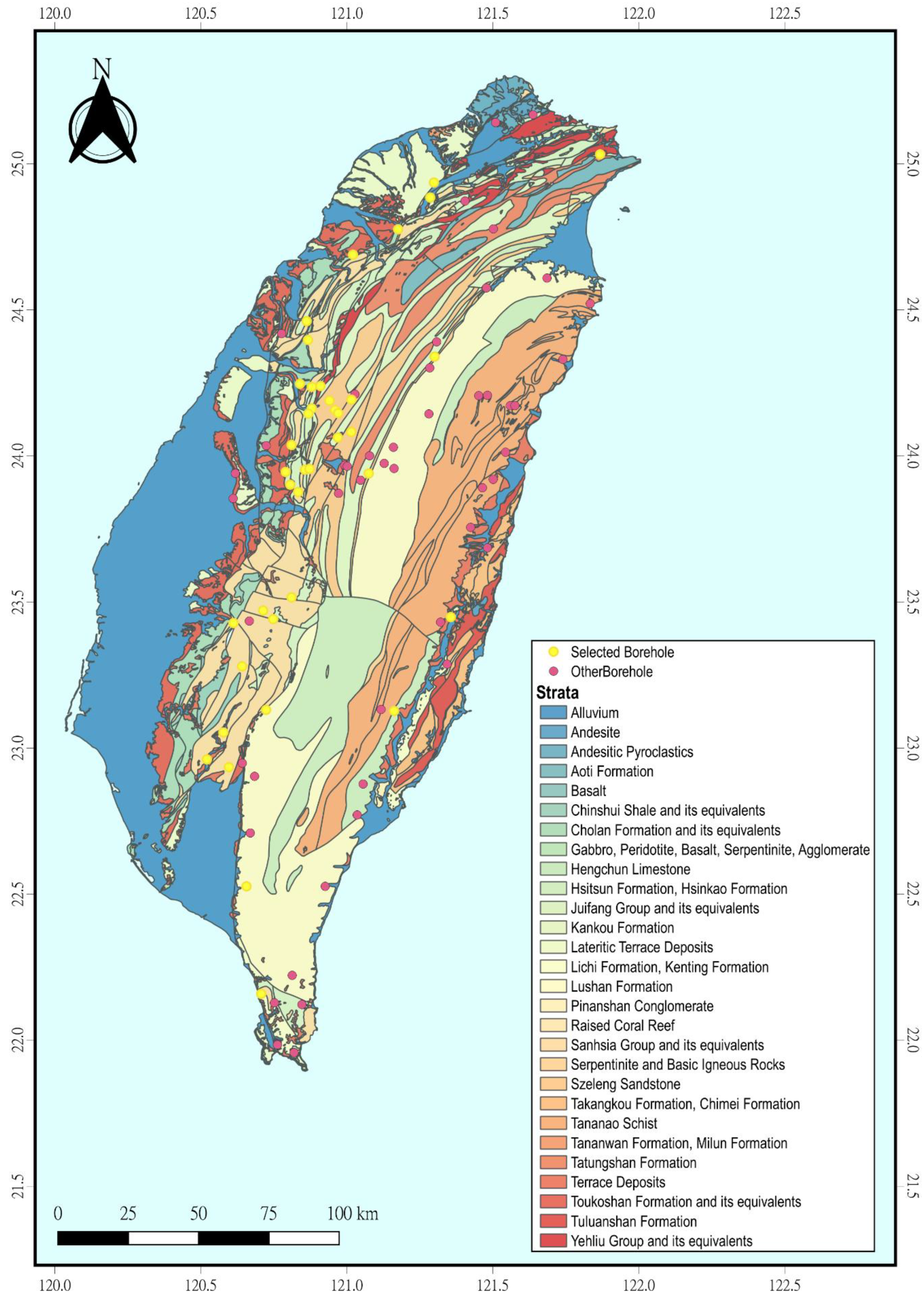
Figure 2.
Flowchart for investigating electrical-hydraulic conductivity relationships.
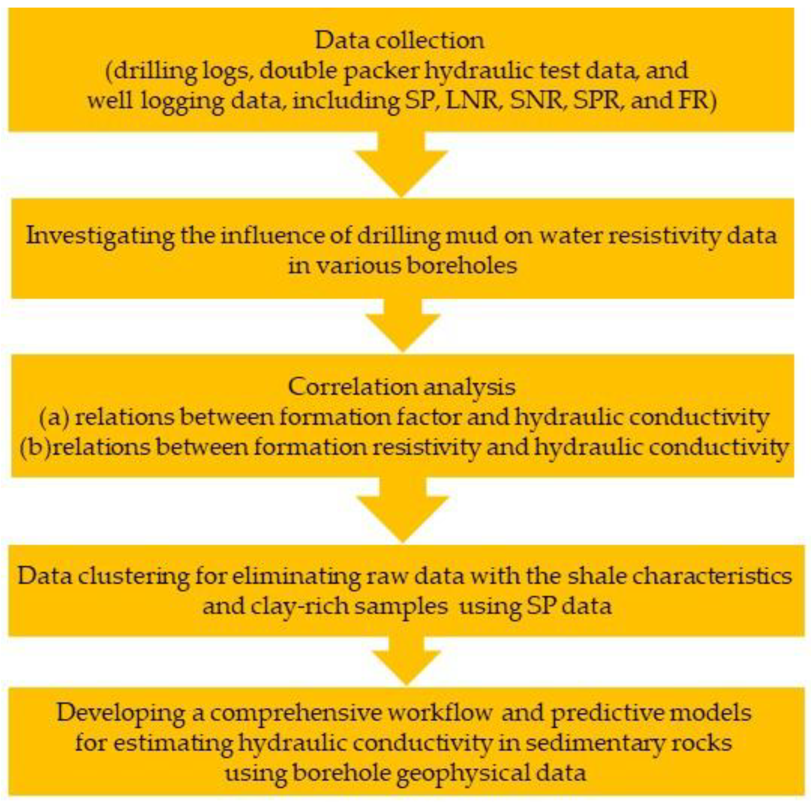
Figure 3.
The fluid resistivity profiles with two distinct distribution patterns. (a) decreasing profile with depth. (b) constant profile with depth.
Figure 3.
The fluid resistivity profiles with two distinct distribution patterns. (a) decreasing profile with depth. (b) constant profile with depth.
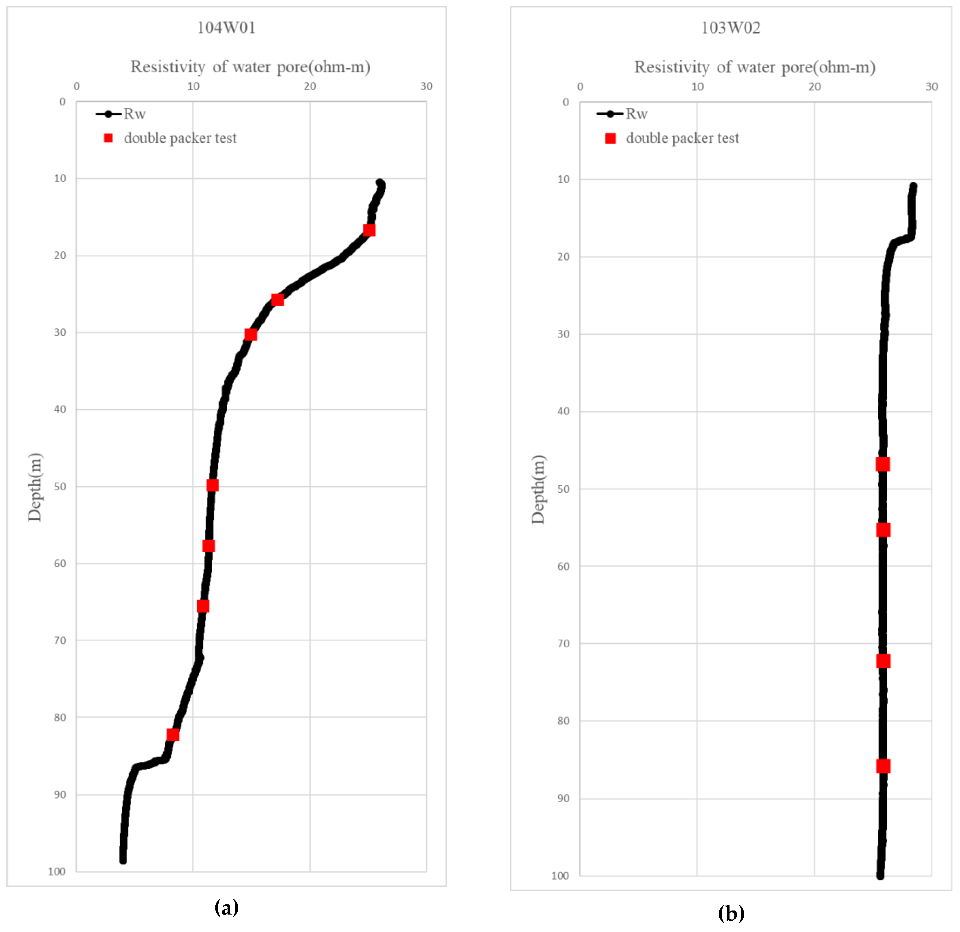
Figure 4.
Histogram of SP for two lithologies (sandstone and shale, respectively).
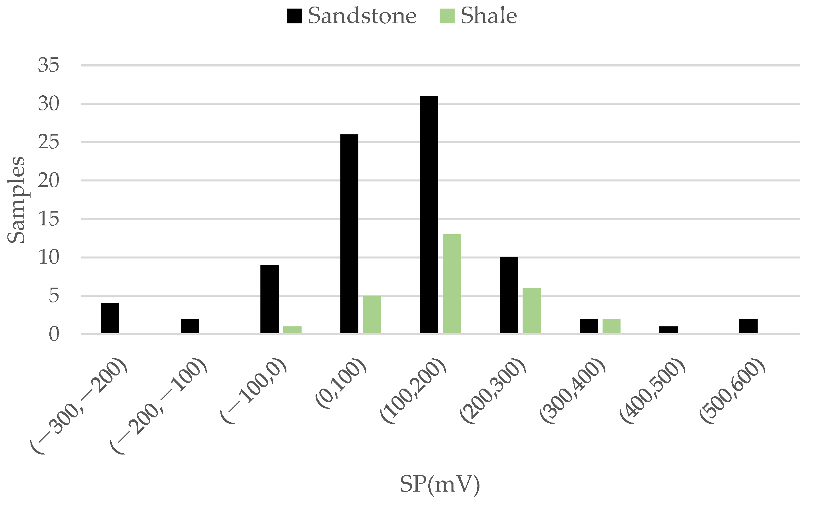
Figure 5.
Regression analysis outcome for Model S1.
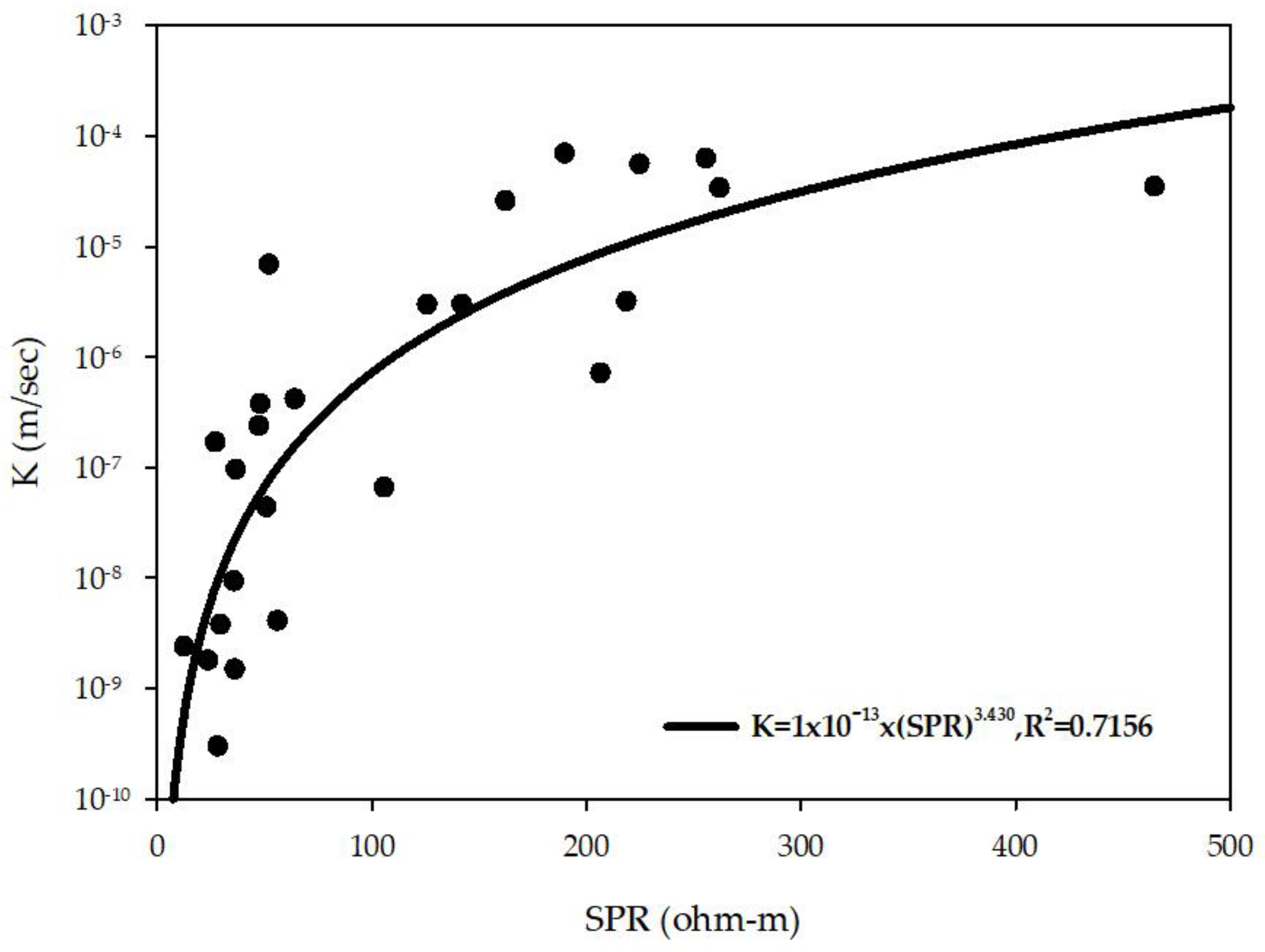
Figure 6.
Regression analysis outcome for Model S2.
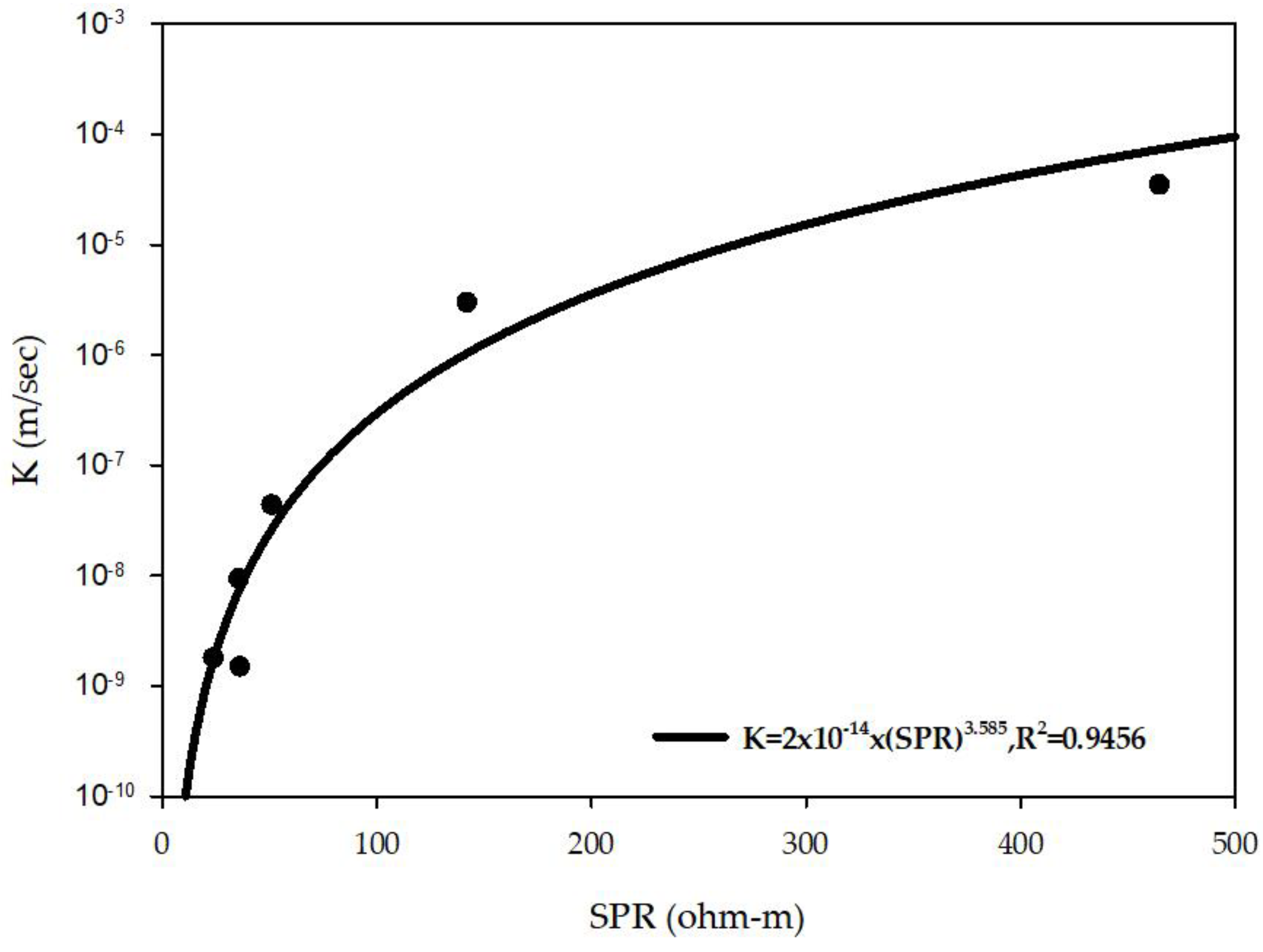

Table 1.
Types of anomalies in various well-logging signals.
| Type of signals | Abnormal patterns |
| SP | −99999, −999, 5062 |
| SNR | Negative value, 12000, 0 |
| LNR | Negative value, 12000, 0 |
| SPR | Negative value, 12000, 0 |
| FR | Negative value, 0, 657 |
Table 2.
Correlation coefficient (r) between geophysical signals and K for sandstone, shale, and sedimentary rocks.
Table 2.
Correlation coefficient (r) between geophysical signals and K for sandstone, shale, and sedimentary rocks.
| Sandstone | Shale | Sedimentary Rocks | |
| Samples | 87 | 27 | 114 |
| SNR | 0.45 | 0.525 | 0.489 |
| LNR | 0.37 | 0.453 | 0.427 |
| SPR | 0.458 | 0.482 | 0.48 |
| SP | −0.119 | 0.022 | −0.077 |
| FR | 0.310 | 0.288 | 0.331 |
Table 3.
Correlation coefficients (r) between resistivity signals/formation factor and K in sedimentary rocks dataset.
Table 3.
Correlation coefficients (r) between resistivity signals/formation factor and K in sedimentary rocks dataset.
| Resistivity | r | Formation factor | r |
| SNR | 0.45 | FS (SNR/FR) | 0.164 |
| LNR | 0.37 | FL(LNR/FR) | 0.079 |
| SPR | 0.458 | FP(SPR/FR) | 0.13 |
Table 4.
Correlation coefficient (r) between various resistivity signals and K in sedimentary rocks under different filtering intervals of SP values.
Table 4.
Correlation coefficient (r) between various resistivity signals and K in sedimentary rocks under different filtering intervals of SP values.
| Selected interval of SP values | Unfiltered | < 0 | > 0 | (−100,0) | (0,100) | (100,200) | (0,60) | (−100,60) |
| Sample quantity |
114 | 16 | 98 | 10 | 31 | 44 | 15 | 25 |
| r(SNR) | 0.489 | 0.547 | 0.482 | 0.503 | 0.583 | 0.263 | 0.75 | 0.714 |
| r(LNR) | 0.427 | 0.200 | 0.462 | 0.115 | 0.607 | 0.248 | 0.639 | 0.518 |
| r(SPR) | 0.480 | 0.656 | 0.476 | 0.879 | 0.583 | 0.316 | 0.804 | 0.858 |
Table 5.
Coefficient of determination (R²) between SPR and K under different filtering intervals of ΔSP values.
Table 5.
Coefficient of determination (R²) between SPR and K under different filtering intervals of ΔSP values.
| ΔSP (mv) | R2 | Sample quantity |
| N.A. | 0.7156 | 25 |
| > 5 | 0.8559 | 15 |
| (5,30) | 0.8664 | 13 |
| (5,20) | 0.8600 | 12 |
| (5,15) | 0.8908 | 9 |
| (5,10) | 0.9456 | 6 |
Table 6.
Evaluation results for S1 and S2 models.
| Models |
Independence (D–W statistic) |
Normality (K-S Statistic/P–values) |
Constant of Variance (Spearman/P–values) |
F test statistic | |
| F ratio | P–values | ||||
| S1 | 2.010 | 0.894 | 0.942 | 58.098 | <0.0001 |
| S2 | 1.210 | 0.852 | 0.787 | 65.094 | 0.001 |
Disclaimer/Publisher’s Note: The statements, opinions and data contained in all publications are solely those of the individual author(s) and contributor(s) and not of MDPI and/or the editor(s). MDPI and/or the editor(s) disclaim responsibility for any injury to people or property resulting from any ideas, methods, instructions or products referred to in the content. |
© 2025 by the authors. Licensee MDPI, Basel, Switzerland. This article is an open access article distributed under the terms and conditions of the Creative Commons Attribution (CC BY) license (http://creativecommons.org/licenses/by/4.0/).
Copyright: This open access article is published under a Creative Commons CC BY 4.0 license, which permit the free download, distribution, and reuse, provided that the author and preprint are cited in any reuse.


