Submitted:
06 October 2025
Posted:
08 October 2025
You are already at the latest version
Abstract
Motivated by recent efforts in simulating nonequilibrium scenarios of the Dicke model in quantum-gas cavity QED, we investigate direct probing of the normal-to-superradiant quantum phase transition via quantum Fisher information (QFI). This transition represents a paradigmatic example of spontaneous symmetry breaking in quantum optics, where the system’s continuous U(1) symmetry is broken in the superradiant phase. At zero temperature, we derive analytical expressions for the QFI in the limit where the atomic transition frequency—scaled by the cavity frequency—tends to infinity. Furthermore, we analyze the impact of finite temperature on the QFI in both the thermodynamic limit and the regime of a finite but large number of atoms. All results demonstrate that the QFI exhibits a singularity as the coupling crosses the critical point—a clear signature of quantum criticality associated with spontaneous symmetry breaking. The divergent behavior of the QFI across the quantum phase transition directly relates to measuring dynamic susceptibilities using experimentally accessible Bragg spectroscopy tools and resources.
Keywords:
Dicke model
; quantum Fisher information
; quantum phase transition
; superradiant phase
; Bragg spectroscopy
; symmetry breaking
1. Introduction
Light–matter interactions are the cornerstone of quantum information processing and quantum state engineering—a theme underscored in numerous reviews [1,2,3,4]. Quantum-gas cavity QED (cavity-QED) [5,6] now leads the way in unraveling and controlling such interactions. Unlike conventional quantum optics, cavity-QED is defined by two defining features [5,6]: repeated light-atom coupling to the *same* atomic ensemble, and the backaction of atoms on the light field—both of which govern the collective dynamics. Consequently, cavity-QED hosts exotic nonclassical phenomena—making it an ideal platform for quantum metrology [7,8]. Moreover, its nondestructive probing via cavity leakage photons positions cavity-QED as a unique system for exploring non-equilibrium many-body phases, yielding insights inaccessible in traditional condensed-matter physics [9].
Within this research thread, simulating nonequilibrium Dicke model scenarios in cavity-QED has emerged as a focal topic [5,6]. The Dicke model exhibits a rich symmetry structure, with a normal phase preserving the U(1) symmetry and a superradiant phase where this symmetry is spontaneously broken. A landmark theoretical proposal [13] put forward realizing an open Dicke model via cavity-assisted Raman transitions, aiming to characterize the associated superradiant phase transition. Building on this concept [13], experiments with Bose-Einstein condensates (BECs) coupled to high-finesse cavities linked self-organization to the Dicke model—and observed the phase transition [14,15,16,17,18]. Yet, directly measuring quantum phases across the critical point in experiments remains a persistent challenge. Theoretical works [19,20,21,22] proposed using entanglement as a quantifier for quantum phase transitions, via density matrix tomography. For few-atom optical lattices, protocols leveraging atomic physics tools—single-site manipulation and readout—measure entanglement entropy and state purity by replicating the quantum system. However, a key limitation is their exponential resource scaling, which restricts these approaches to small system sizes.
In this work, we propose a method to characterize the Dicke model’s quantum phase transition (QPT) in cavity-QED—specifically across the critical point—using experimentally accessible tools. Our approach leverages the quantum Fisher information (QFI), a quantity directly connectable to dynamic susceptibility measurements via Bragg spectroscopy (a technique with experimental reach). Importantly, the QFI serves as a sensitive probe of symmetry breaking phenomena, as it captures the system’s sensitivity to parameter variations near critical points where symmetries are spontaneously broken. At zero temperature, we derive analytical QFI expressions in the limit where the atomic transition frequency (scaled by the cavity frequency) tends to infinity. We additionally analyze finite-temperature QFI effects in both the thermodynamic limit and for large but finite atom numbers. All results show a singularity in the QFI as coupling increases across the critical point—a distinct signature of quantum criticality. This divergent QFI behavior during the phase transition directly relates to measuring dynamic susceptibilities with Bragg spectroscopy, bridging theoretical predictions to experimental practice.
This paper is structured as follows. In Section 2, we introduce the model system—where the self-organization phase transition corresponds to a subradiant quantum phase transition involving spontaneous symmetry breaking. In Section 3, we show how the QFI serves as an efficient probe for dynamic Dicke superradiance in a BEC coupled to an optical cavity. Finally, in Section 4, we discuss experimental accessibility of the described phenomena and conclude with a summary of our work.
2. Model Hamiltonian and Quantum Fisher Information
We study a BEC of N atoms (mass m) confined in a cavity of length L [14,15,16,17,18]. Their internal motion couples to a cavity mode (operator , frequency ). We describe the bosonic matter-wave field () using a two-mode momentum expansion [19]: specifically, . Using the Schwinger representation, we define spin components: and . The resulting effective Hamiltonian maps to a Dicke-like model, as detailed in Ref. [19]:
In this Hamiltonian, are the Pauli matrices for the two-mode bosonic field (Schwinger representation), and () denotes the cavity annihilation (creation) operator. The recoil frequency is . The tunable detuning combines the atom-pump detuning , which we tune via the pump laser frequency . The coupling strength is controlled by the transverse driving amplitude —here, is the transverse driving Rabi frequency, the single-photon Rabi frequency at the cavity antinode, and the atom-pump detuning ( = atomic resonance frequency). Note that the last term in Eq. (1) is small () and often negligible in cavity QED.
The Dicke-like Hamiltonian (Eq. 1) describes the interplay between N two-level atoms and a single bosonic mode, building on Dicke’s seminal work [10]. This model is known to host a quantum phase transition (QPT) from the normal to superradiant phase as atom-field coupling strengthens [11,12,19]. Specifically, for coupling strength , the system remains in the normal phase; for , it transitions to the superradiant phase.
Here, we use quantum Fisher information (QFI) to characterize this normal-to-superradiant QPT in the Eq. (1) Hamiltonian—a direct probe for symmetry-breaking phenomena. The QFI, denoted , quantifies the distinguishability between a density matrix and its unitary transform —induced by a Hermitian operator with small phase . For a pure state , QFI is given by [23,24,25,26,27,28]:
For a mixed state in thermal equilibrium, the QFI is expressed as [23,24,25,26,27,28]:
where represents the occupation probability in the energy eigenbasis , with Z being the partition function.
The key idea behind the utility of QFI to detect the quantum phase transition can be explained as follows: when one adiabatically drives the system across the critical point, a divergent Fisher information is expected to occur [29]. This effectiveness stems from the closing of the energy gap above the ground state during continuous quantum phase transitions in the thermodynamic limit. Consider the ground state of a Hamiltonian . The impact of a vanishing energy gap on the quantum Fisher information, as given by Eq. (2), becomes evident from the expression:
Clearly, as the energy gap above the ground state narrows in the denominator, the quantum Fisher information soars. This property potentially enables arbitrarily high precision in measuring phase transitions in the thermodynamic limit. In the subsequent sections, we will explore the quantum phase transitions of the Hamiltonian described by Eq. (1) by calculating the QFI using Eqs. (2) and (3).
It’s worth noting that while Ref. [29] also employed QFI as an indicator of the superradiant quantum phase transition, our current work differs in several key aspects: (i) The light-matter coupling inherent in our practical experimental setup is complex, whereas the one examined in Ref. [29] is real. This necessitates a distinct approach to analyzing the Hamiltonian at finite temperatures, as reflected in Eq. (12). (ii) We obtain analytical expressions for the QFI at zero temperature, rather than relying solely on numerical solutions, which were not provided in Ref. [29]. Thus, our study, in conjunction with Ref. [29], offers a comprehensive framework for using the QFI to probe the symmetry-breaking quantum phase transition of the Dicke-like Hamiltonian.
3. Probing Quantum Phase Transition of Hamiltonian (1) via QFI
3.1. QFI at Zero Temperature
In this section, we utilize the Quantum Fisher Information (QFI) given in Eq. (2) to explore the quantum phase transition occurring at zero temperature, specifically within the limit where . For clarity, let’s denote the eigenstates of as and the eigenstates of as .
To commence our investigation, we calculate the QFI linked to the normal phase of the Hamiltonian (1) in the range of . We employ a strategy that involves seeking a unitary Schrieffer-Wolff transformation [30]. This transformation, given by , decouples the two spin subspaces (namely, and ) in the transformed Hamiltonian . As a result, we derive the effective low-energy form of the Hamiltonian (1) in its normal phase:
The eigenvalues and eigenstates of this effective Hamiltonian can be determined analytically. The eigenvalues of the Hamiltonian (5) are given by:
where . The corresponding eigenstates, related to Eq. (6), can be represented as . Here, is the squeezing operator, with as the squeezing parameter.
Note that the eigenvalues in Eq. (6) are real only when the atom-field coupling y is less than or equal to the critical value , and they vanish precisely at this critical point. For the parameter range where , we can substitute the derived and the corresponding eigenstates into Eq. (2). This allows us to obtain the analytical expression for Quantum Fisher Information (QFI), given by:
From Eq. (7), it is evident that QFI diverges as y approaches , indicating a quantum phase transition. Importantly, Eq. (2) is not applicable for .
Moving on, we explore the QFI associated with the superradiant phase of the model Hamiltonian (1) for . In this phase, the number of photons within the cavity field becomes proportional to N. To capture the essential low-energy physics, we apply a similarity transformation to the Hamiltonian (1). Here, is the displacement operator, and represents a rotation transformation [19,30]. By choosing and , we obtain the effective low-energy form of the Hamiltonian (1) in the superradiant phase:
where , , and . Equation (8) bears structural similarity to the original Hamiltonian (1), but with rescaled parameters and . This allows us to routinely derive the eigenstates of Eq. (8) as , with . The corresponding eigenvalue is given by:
For the standard parameters where , , and , the eigenvalue expressed in Eq. (9) corresponds to that of the Hamiltonian (8) in the superradiant phase. This eigenvalue is real only if y surpasses the critical value . Based on Eq. (2), we can derive the analytical expression for Quantum Fisher Information (QFI) in the super-radiant phase as follows:
It’s worth noting that in the regime where , the advanced corrections in Eqs. (5) and (8) become negligible [30]. Consequently, from Eq. (5) and from Eq. (8) emerge as the precise low-energy effective Hamiltonians for the normal phase () and the superradiant phase () respectively. This implies that Equations (7) and (10) precisely represent the QFI of the Hamiltonian (1) in its respective phases.
Leveraging Equations (7) and (10), we can devise a method to detect the quantum phase transition inherent in the Hamiltonian (1). Let’s explore some pivotal characteristics of this transition and its relationship to QFI as defined in Eq. (2). Firstly, the rescaled cavity photon count, denoted as , serves as an order parameter. It remains zero when and becomes finite, with a value of , when . Secondly, the rescaled ground state energy, computed as , demonstrates continuity at the critical point . However, a discontinuity arises in its second derivative, highlighting the second-order nature of the quantum phase transition. Thirdly, as we approach the critical point, the excitation energies in both phases vanish, proportional to and as indicated by Eqs. (6) and (9). Consequently, the QFI (2) diverges in a manner proportional to , aligning with the findings of Eqs. (7) and (10). This divergence is a hallmark of critical behavior associated with symmetry breaking, where the system’s response to external perturbations becomes singular. In Figure 1 (a) and (b), we illustrate the outcomes for QFI and its first derivative based on Equations (7) and (10). The red solid curves prominently showcase the divergence of QFI at the critical point , a direct consequence of the narrowing energy gap above the ground state as expressed in Eq. (4). In contrast, both QFI and its first derivative rapidly diminish to zero when y moves away from . This trend can be understood through Eq. (2). When the system is not in the vicinity of the quantum phase transition’s critical point, it becomes highly resistant to external perturbations represented by . As a result, approaches unity, indicating a negligible QFI according to Eq. (2). Finally, it’s worth mentioning that the QFI depicted in Figure 1 (a) and its first derivative in Figure 1 (b) can be empirically determined by analyzing the squared Hellinger distance between probability distributions, as outlined in Ref. [28].
3.2. The QFI at Finite Temperatures
In Section 3.1, we analytically derived the QFI for the Hamiltonian (1) at zero temperature, as seen in Eqs. (7) and (10). Now, in this Section 3.2, our intention is to explore the influence of finite temperature on the QFI, utilizing Eq. (3), particularly in the thermodynamic limit where N and V tend to infinity while maintaining a constant atom density .
Drawing from the work presented in Ref. [19], we adopt the Holstein-Primakoff transformation, specifically, and , to recast the atomic freedoms in terms of the bosonic operator . Through this lens, the Hamiltonian (1) can be reframed as:
This reformulated Hamiltonian (11) elegantly describes the dynamics between two intertwined harmonic oscillators, denoted by the operators and respectively.
Shifting our focus to the system’s normal phase, we introduce the position and momentum operators defined as and . Through this lens, Hamiltonian (11) transforms into:
Here, corresponds to and equals . In contrast to the original Dicke-model Hamiltonian explored in Ref. [29], which emphasized the coupling of coordinates with coordinates, Eq. (12) showcases a coupling between coordinates and momenta (evident in the penultimate term of Eq. (12)). This distinction necessitates a fresh approach in analyzing the Hamiltonian, distinct from the methodologies employed in Ref. [29].
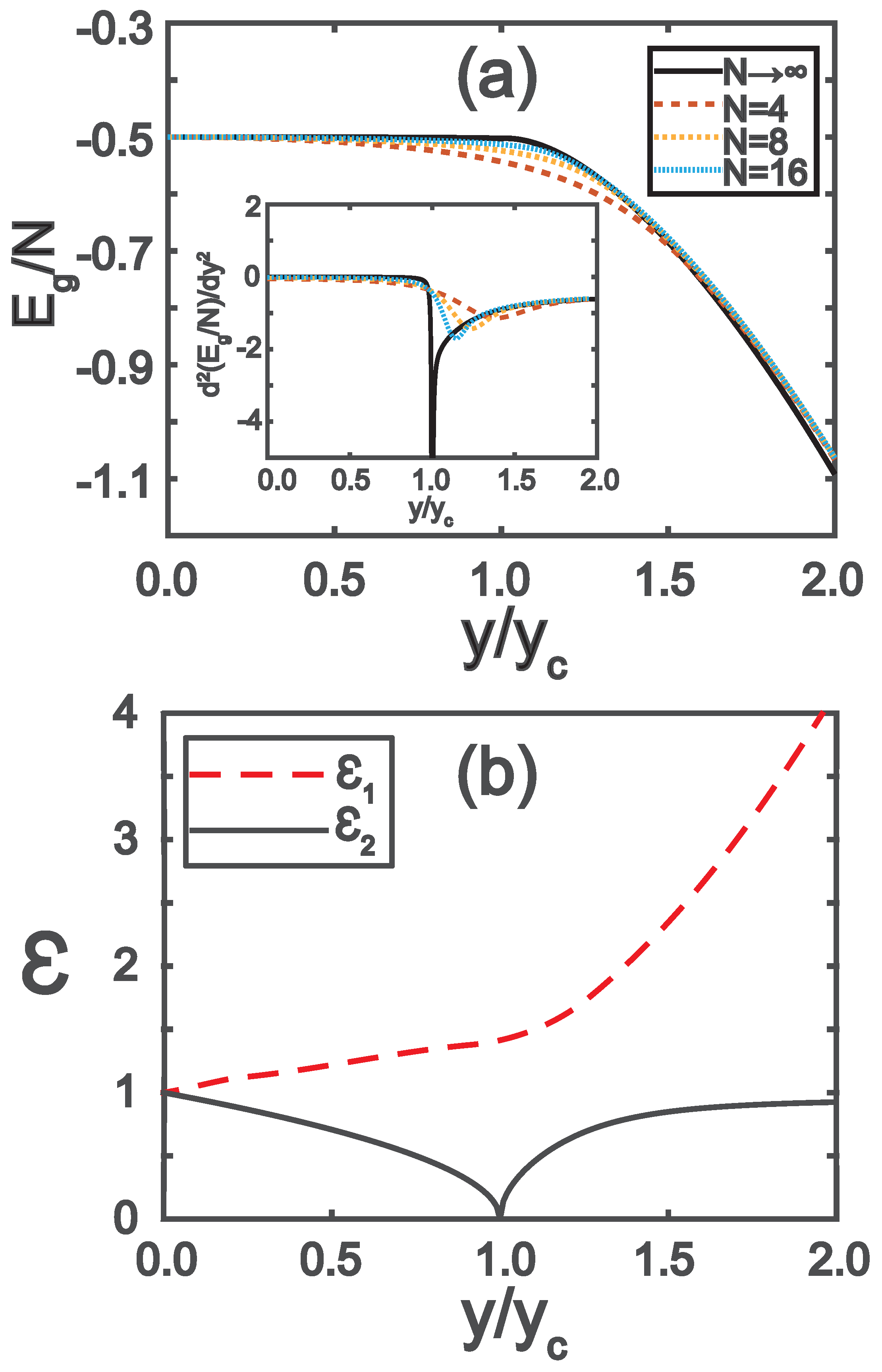
In order to compute the QFI based on Eq. (3) in relation to the normal phase, obtaining the density matrix of from Eq. (3) in the energy basis is crucial. We achieve this by following a three-step process: (i) Firstly, we decouple the two harmonic oscillators in Hamiltonian (12) using Bogoliubov’s transformations. The excitation energies () are determined as . With this knowledge, we can plot the ground state energy and excitation energies, represented by solid black curves in Figure 2 (a) and (b) respectively. It’s worth noting that the ground state energy remains continuous across the critical point, whereas the second derivative of the ground state energy diverges, serving as an indicator of the superradiant quantum phase transition. (ii) Secondly, we obtain the reduced density matrix of the atoms in spatial coordinates as follows:
where , , , , and . (iii) Finally, we derive the eigenvalues of the population corresponding to the energy eigenstate in Eq. (3) as .
Subsequently, one can calculate the squeezing parameter of the atoms, given by . The detailed variances are expressed as:
Consequently, the squeezing parameter is:
depicted by the solid black curves in Figure 1 (c). As anticipated, diverges at the critical point of the quantum phase transition.
Now we are ready to calculate the QFI associated with the normal phase. If we choose as the phase-shift generator, we can obtain the corresponding QFI as follows
For a different choice , we can obtain the corresponding QFI . Obviously, it is better to choose as the phase-shift generator due to , and the corresponding QFI is given by Eq. (16), which has been plotted into the solid black curves in Figure 1 (a) and (b). As is expected, QFI is divergent across the critical point of the quantum phase transition.
We proceed to compute the Quantum Fisher Information (QFI) in the superradiant phase. In this phase, considering the population inversion that occurs across a multitude of atoms, one can decompose the operators and from Hamiltonian (11) as follows:
Here, and represent the mean-field components, while and denote the quantum fluctuations for each subsystem. For clarity, we’ll adopt the notation and , noting that both choices of shifts yield consistent results. There exist a pair of real values for and that eliminate the linear terms in the Hamiltonian (11) within the displaced phase space. These values are determined by:
The trivial solution, where , corresponds to the normal phase. For the non-trivial case where and , a physically meaningful solution arises:
This solution exists within the range if and only if y exceeds , defined as . By approximating the Hamiltonian (11) to the second order and substituting Eq. (19) into it, we obtain the effective Hamiltonian in the superradiant phase at finite temperature:
where the coefficients and ground state energy are defined as follows: , , , , and
Utilizing Eq. (21), we have plotted the ground state energy and its second derivative, depicted as solid black curves in Figure 2 (a). As shown in the inset of Figure 2 (a), the second derivative of the ground state energy diverges at the critical point of , as expected.
Similar to the treatment in the normal phase, we typically introduce operators and , where and . Then, by defining and , we rewrite Hamiltonian (20) as follows:
Equation (22) has the same structure as Eq. (12) with the rescaled frequencies and coupling coefficient, , and . Therefore, by employing the same procedure used to derive , we find the eigenvalues of the density operator as , where , and with , and . We proceed to calculate the analytical expression of the squeezing parameter in the superradiant phase at the finite temperature
which is routine to be plotted into Figure 1 (c). Again, the squeezing parameter is divergent as as a signature of the superradiant quantum phase transition.
Lastly, we compute the Quantum Fisher Information (QFI) of atoms in the superradiant phase at finite temperature. Choosing as the phase-shift generator yields the corresponding QFI:
3.3. Probing Quantum Phase Transition of a Quantum-Gas Cavity QED by Quantum Fisher Information
In Section 3.1 and Section 3.2, we analytically derived the quantum Fisher information (QFI) for the Hamiltonian in Eq. (1)—at zero temperature [Eqs. (7), (10)] and finite temperature in the thermodynamic limit [Eqs. (16), (24)]. In Section 3.3, we extend this to finite atom numbers by numerically computing QFI via Eq. (3) and analyzing its use for detecting quantum phase transitions (QPTs) in quantum-gas cavity QED.
To compute QFI numerically, we first find the eigenvalues and eigenvectors of the density operator . Using the method of Ref. [29], we solve for the ground state of the finite-N Hamiltonian (Eq. 1), where N is the cutoff photon number. We minimize Eq. (1) to obtain , then trace out the bosonic field to get the atomic density operator: . With , we compute its eigenvalues/eigenvectors for and substitute into Eq. (3). We plot QFI (Figure 1(a,b)) and ground-state energy (Figure 2(a)) from these numerics.
Utilizing the data presented in Figure 1 and Figure 2, we are poised to devise a methodology for detecting quantum phase transitions in the Hamiltonian of Eq. (1) through QFI. Let’s highlight some key aspects of the quantum phase transition and QFI as defined in Eq. (2). Firstly, the rescaled cavity photon number, denoted as , serves as an order parameter. It vanishes for and becomes finite with for . This order parameter directly reflects the symmetry breaking. Secondly, the rescaled ground state energy approaches a limit as , indicating continuity at the critical point , as illustrated in Figure 2(a). However, the second derivative of the ground state energy exhibits a discontinuity, as evidenced by the inset curves of Figure 2(a), revealing the second-order nature of the quantum phase transition. Thirdly, in proximity to the critical point, as demonstrated in Eqs. (7) and (10), the excitation energies in both the normal and superradiant phases tend to zero, proportional to as shown in Figure 2(b). Consequently, the QFI in Eq. (2) is expected to diverge as , which is corroborated by Eqs. (7) and (10).
Figure 1(a) is the heart of our QPT detection: it shows QFI for the Eq. (1) Hamiltonian. Solid red/black curves are thermodynamic-limit (, fixed) analytical QFI for zero/finite temperature; dashed curves are numerical QFI for finite N. As N grows, numerical QFI converges to the thermodynamic limit—matching our analytics. Most critically, both approaches show QFI **diverging at **—unambiguous proof of the superradiant quantum phase transition.
4. Discussion and Conclusions
The emphasis and purpose of this work is to design a protocol using QFI to characterize the symmetry-breaking quantum phase transition (QPT) of the Dicke model in cavity QED—specifically across its critical point—relying on experimentally accessible tools. Validating this physics requires experimentally implementing cavity QED, which hinges on tightly controlled light-matter interactions [1,2,3,4]. A prototypical setup uses a Bose-Einstein condensate (BEC) in an optical cavity, where effective atom-field coupling is tuned by varying pump laser intensity over time. Notably, while this cold-atom approach has unique benefits, our results extend to quantum well waveguide implementations, where light-matter interaction can be activated in less than a light cycle [31].
Our methodology to characterize the Dicke model’s quantum phase transition (QPT) in cavity QED across the critical point leverages quantum Fisher information (QFI) measurements. Experimentally, QFI—at zero and finite temperatures—can be extracted via dynamic susceptibility measurements using Bragg spectroscopy, a technique established in cold-atom and condensed-matter systems [27]. Alternatively, QFI and its first derivative can be extracted by extrapolating polynomial fits to the squared Hellinger distance between probability distributions, as proposed in Ref. [28].
With these experimental pathways in place, the phenomena we study should be accessible with current capabilities. We restrict our analysis to the Schrieffer-Wolff transformation (valid for at zero temperature) and the Holstein-Primakoff approximation (thermodynamic limit, finite temperature). For regimes beyond these approximations, the functional path integral method is reliable but lies outside our scope [12].
In summary, we use the QFI to characterize the symmetry-breaking quantum phase transition in the cavity-QED Dicke model across the critical point. At zero temperature, we derive analytical QFI expressions for the limit where the atomic transition frequency (scaled by the cavity frequency) tends to infinity. We also analyze finite-temperature QFI effects in the thermodynamic limit and for large but finite atom numbers. Consistently, we find a QFI singularity as coupling crosses the critical point—a distinct signature of quantum criticality. This divergent QFI behavior correlates directly with dynamic susceptibility measurements via Bragg spectroscopy—an accessible experimental tool.
Author Contributions
Conceptualization, Z.L.; Investigation, L.Z.; Methodology, L.Z. and Z.L.; soft- ware, Q.W.; writing—original draft preparation, L.Z.; writing—review and editing, Z.L.; supervision, Z.L.; All authors have read and agreed to the published version of the manuscript.
Funding
This work was supported by the National Natural Science Foundation of China (Grants No. 12574301) and the Zhejiang Provincial Natural Science Foundation (Grant No. LZ25A040004).
Data Availability Statement
Data is contained within the article.
Acknowledgments
We thank Guangri Jin and Ying Hu for stimulating discussions and helpful assistance, as well as Professor Yanhong Xiao for her insightful guidance.
Conflicts of Interest
The authors declare no conflicts of interest.
References
- Hammerer, K.; Sørensen, A.S.; Polzik, E.S. Quantum interface between light and atomic ensembles. Rev. Mod. Phys. 2010, 82, 1041. [CrossRef]
- Forn-Díaz, P.; Lamata, L.; Rico, E.; Kono, J.; Solano, E. Ultrastrong coupling regimes of light-matter interaction. Rev. Mod. Phys. 2019, 91, 025005. [CrossRef]
- Frisk Kockum, A.; Miranowicz, A.; De Liberato, S.; Savasta, S.; Nori, F. Ultrastrong coupling between light and matter. Nat. Rev. Phys. 2019, 1, 19. [CrossRef]
- Liu, J.; Liu, M.; Ying, Z.J.; Luo, H.G. Fundamental Models in the Light–Matter Interaction: Quantum Phase Transitions and the Polaron Picture. Adv. Quantum Technol. 2021, 4, 2000139. [CrossRef]
- Ritsch, H.; Domokos, P.; Brennecke, F.; Esslinger, T. Cold atoms in cavity-generated dynamical optical potentials. Rev. Mod. Phys. 2013, 85, 553. [CrossRef]
- Mivehvar, F.; Piazza, F.; Donner, T.; Ritsch, H. Cavity QED with quantum gases: new paradigms in many-body physics. Adv. Phys. 2021, 70, 1. [CrossRef]
- Pezzè, L.; Smerzi, A.; Oberthaler, M.K.; Schmied, R.; Treutlein, P. Quantum metrology with nonclassical states of atomic ensembles. Rev. Mod. Phys. 2018, 90, 035005. [CrossRef]
- Polino, E.; Valeri, M.; Spagnolo, N.; Sciarrino, F. Photonic quantum metrology. AVS Quantum Sci. 2020, 2, 024703. [CrossRef]
- Gross, C.; Bloch, I. Quantum simulations with ultracold atoms in optical lattices. Science 2017, 357, 995. [CrossRef]
- Dicke, R.H. Coherence in Spontaneous Radiation Processes. Phys. Rev. 1954, 93, 99. [CrossRef]
- Hepp, K.; Lieb, E.H. On the superradiant phase transition for molecules in a quantized radiation field: the dicke maser model. Ann. Phys. 1973, 76, 360. [CrossRef]
- Wang, Y.K.; Hioe, F.T. Phase Transition in the Dicke Model of Superradiance. Phys. Rev. A 1973, 7, 831. [CrossRef]
- Dimer, F.; Estienne, B.; Parkins, A.S.; Carmichael, H.J. Proposed realization of the Dicke-model quantum phase transition in an optical cavity QED system. Phys. Rev. A 2007, 75, 013804. [CrossRef]
- Baumann, K.; Guerlin, C.; Brennecke, F.; Esslinger, T. Dicke quantum phase transition with a superfluid gas in an optical cavity. Nature(London) 2010, 464, 1301. [CrossRef]
- Baumann, K.; Mottl, R.; Brennecke, F.; Esslinger, T. Exploring Symmetry Breaking at the Dicke Quantum Phase Transition. Phys. Rev. Lett. 2011, 107, 140402. [CrossRef]
- Baden, M.P.; Arnold, K.J.; Grimsmo, A.L.; Parkins, S.; Barrett, M.D. Realization of the Dicke Model Using Cavity-Assisted Raman Transitions. Phys. Rev. Lett. 2014, 113, 020408. [CrossRef]
- Kongkhambut, P.; Keßler, H.; Skulte, J.; Mathey, L.; Cosme, J.G.; Hemmerich, A. Realization of a Periodically Driven Open Three-Level Dicke Model. Phys. Rev. Lett. 2021, 127, 253601. [CrossRef]
- Skulte, J.; Kongkhambut, P.; Rao, S.; Mathey, L.; Keßler, H.; Hemmerich, A.; Cosme, J.G. Condensate Formation in a Dark State of a Driven Atom-Cavity System. Phys. Rev. Lett. 2023, 130, 163603. [CrossRef]
- Nagy, D.; Kónya, G.; Szirmai, G.; Domokos, P. Dicke-Model Phase Transition in the Quantum Motion of a Bose-Einstein Condensate in an Optical Cavity. Phys. Rev. Lett. 2010, 104, 130401. [CrossRef]
- Lambert, N.; Emary, C.; Brandes, T. Entanglement and the Phase Transition in Single-Mode Superradiance. Phys. Rev. Lett. 2004, 92, 073602. [CrossRef]
- Emary, C.; Brandes, T. Quantum Chaos Triggered by Precursors of a Quantum Phase Transition: The Dicke Model. Phys. Rev. Lett. 2003, 90, 044101. [CrossRef]
- Emary, C.; Brandes, T. Chaos and the quantum phase transition in the Dicke model. Phys. Rev. E 2003, 67, 066203. [CrossRef]
- Braunstein, S.L.; Caves, C.M. Statistical distance and the geometry of quantum states. Phys. Rev. Lett. 1994, 72, 3439. [CrossRef]
- Pezzé, L.; Smerzi, A. Entanglement, Nonlinear Dynamics, and the Heisenberg Limit. Phys. Rev. Lett. 2009, 102, 100401. [CrossRef]
- Genoni, M.G.; Olivares, S.; Paris, M.G.A. Optical Phase Estimation in the Presence of Phase Diffusion. Phys. Rev. Lett. 2011, 106, 153603. [CrossRef]
- Ma, J.; Huang, Y.x.; Wang, X.; Sun, C.P. Quantum Fisher information of the Greenberger-Horne-Zeilinger state in decoherence channels. Phys. Rev. A 2011, 84, 022302. [CrossRef]
- Hauke, P.; Heyl, M.; Tagliacozzo, L.; Zoller, P. Measuring multipartite entanglement through dynamic susceptibilities. Nat. Phys. 2016, 12, 778. [CrossRef]
- Strobel, H.; Muessel, W.; Linnemann, D.; Zibold, T.; Hume, D.B.; Pezzè, L.; Smerzi, A.; Oberthaler, M.K. Fisher information and entanglement of non-Gaussian spin states. Science 2014, 345, 424. [CrossRef]
- Wang, T.L.; Wu, L.N.; Yang, W.; Jin, G.R.; Lambert, N.; Nori, F. Quantum Fisher information as a signature of the superradiant quantum phase transition. New J. Phys. 2014, 16, 063039. [CrossRef]
- Hwang, M.J.; Puebla, R.; Plenio, M.B. Quantum Phase Transition and Universal Dynamics in the Rabi Model. Phys. Rev. Lett. 2015, 115, 180404. [CrossRef]
- Günter, G.; Anappara, A.A.; Hees, J.; Sell, A.; Biasiol, G.; Sorba, L.; De Liberato, S.; Ciuti, C.; Tredicucci, A.; Leitenstorfer, A.; et al. Sub-cycle switch-on of ultrastrong light–matter interaction. Nature(London) 2009, 458, 178. [CrossRef]
Figure 1.
(a) Scaled quantum Fisher information plotted against the coupling coefficient y. (b) The scaled quantum Fisher information’s first derivative graphed as a function of the coupling coefficient y. (c) Illustration of the spin squeezing parameter for the atoms versus the coupling strength y. Solid lines represent the analytical results of the QFI obtained in the thermodynamic limit, while dashed lines depict numerical outcomes for a finite number of atoms, specifically , 8, 12, and 20. The parameters used are and .
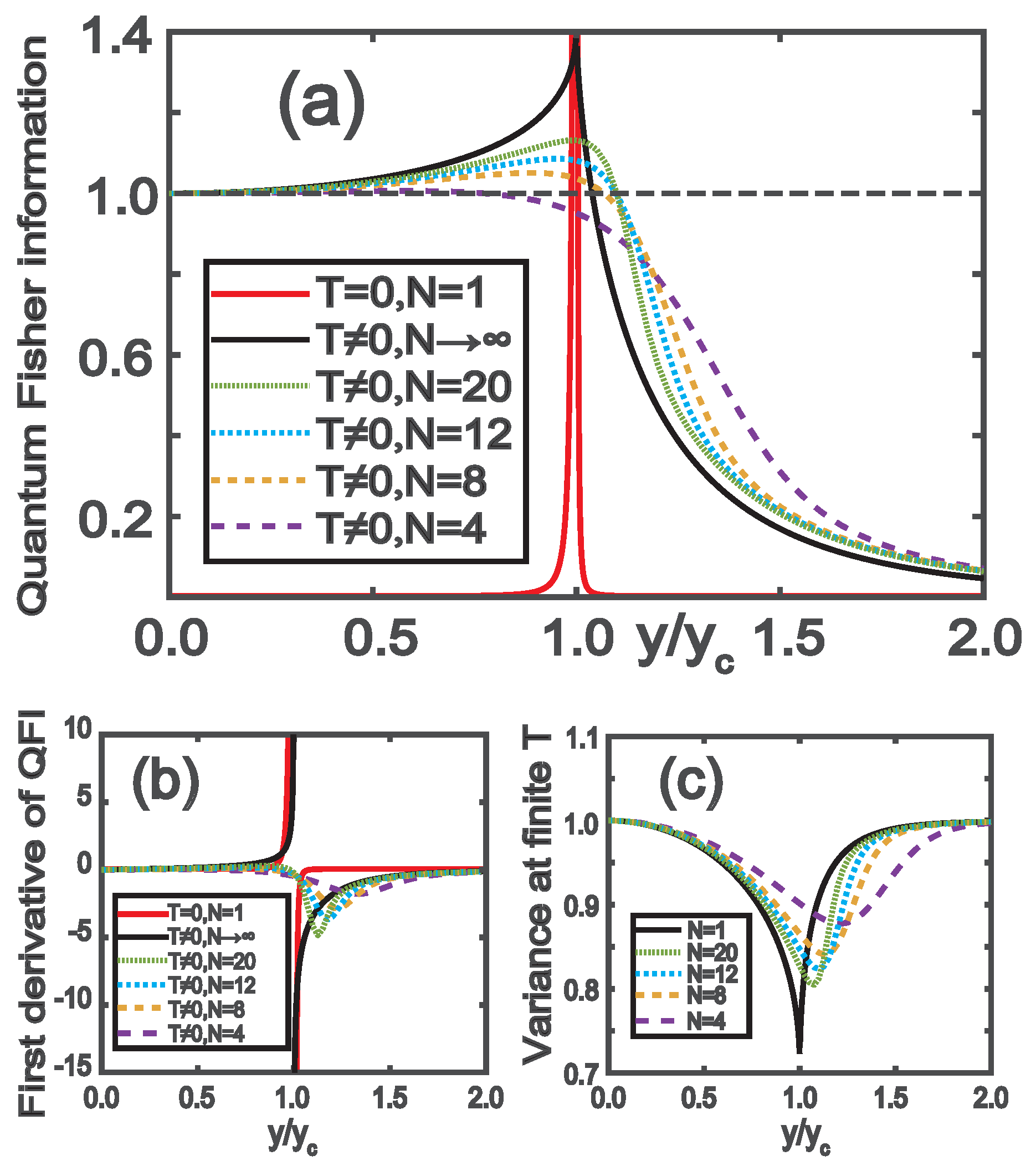
Figure 2.
(a) Ground state energy of Hamiltonian(Eq. (11)) and its second derivative of as a function of the coupling coefficient y. Solid lines: analytical results in the thermodynamic limit(i.e., ). Dashed lines: numerical results for a finite number of the atoms , 8, 16 . (b) Eigenergies of the upper and lower polariton excitations on the Hamiltonian as a function of the coupling coefficient y in the thermodynamic limit. Parameters are chosen as and .
Disclaimer/Publisher’s Note: The statements, opinions and data contained in all publications are solely those of the individual author(s) and contributor(s) and not of MDPI and/or the editor(s). MDPI and/or the editor(s) disclaim responsibility for any injury to people or property resulting from any ideas, methods, instructions or products referred to in the content. |
© 2025 by the authors. Licensee MDPI, Basel, Switzerland. This article is an open access article distributed under the terms and conditions of the Creative Commons Attribution (CC BY) license (http://creativecommons.org/licenses/by/4.0/).
Copyright: This open access article is published under a Creative Commons CC BY 4.0 license, which permit the free download, distribution, and reuse, provided that the author and preprint are cited in any reuse.


