Entropy—Sieve Methods and Energy Functionals in the Erdős Problem [Er79] on Quadratic Prime Representations

1. Notation

Table 1. Notation and assumptions used throughout the paper.

Symbol	Meaning
$\mathbb{N}$	Set of positive integers $\{1,2,3,\dots \}$.
$\mathbb{P}$	Set of prime numbers.
$p,q$	Prime variables.
$a,b$	Integer parameters with $a\ge 1$ and $0\le b<p$.
$[1,x]$	Interval of integers $\{n\in \mathbb{N}:1\le n\le x\}$.
$\Lambda \left(n\right)$	von Mangoldt function.
$P\left(D\right)$	Product of primes less than D: $P\left(D\right)={\prod }_{p<D}p$.
$S(\mathcal{A},\mathcal{P},D)$	Classical sieve count of elements of $\mathcal{A}$ coprime to $P\left(D\right)$.
$\mathcal{E}$	Exceptional set of integers not representable in the form $a{p}^2+b$ (Erdős Problem #676).
M	Canonical modulus $M={\prod }_{p\le Y}{p}^2$ used in entropy–sieve reduction.
$N_r$	Count of integers $n\le x$ with $n\equiv r(modM)$.
$\Delta (x;q,a)$	Discrepancy in an arithmetic progression: $\pi (x;q,a)-{\displaystyle \frac{\pi \left(x\right)}{\phi \left(q\right)}}$.
$V(M;x)$	Nonzero-frequency variance functional: $V(M;x)={\sum }_{amodM,a\ne 0}|{\sum }_{n\le x}e(an/M){|}^2$.
$\mu$	Probability distribution on a finite set $\mathcal{A}\subseteq \mathbb{N}$.
$P,Q$	Respectively the empirical distribution of residues and the uniform reference distribution.
$D(P\parallel Q)$	Kullback–Leibler (KL) divergence of P from Q.
${\mathbb{E}}_{\mu }\left[f\right]$	Expectation of a function f under distribution $\mu$: ${\mathbb{E}}_{\mu }\left[f\right]={\sum }_{n\in \mathcal{A}}f\left(n\right)\mu \left(n\right)$.
$H\left(\mu \right)$	Shannon entropy of $\mu$: $H\left(\mu \right)=-{\sum }_{n\in \mathcal{A}}\mu \left(n\right)log\mu \left(n\right)$.
${\mathcal{E}}_2\left(P\right)$	Quadratic energy functional: ${\mathcal{E}}_2\left(P\right)={\displaystyle \frac{1}{x^2}}{\sum }_{rmodM}{N}_r^2$.
(UH)	Uniformity Hypothesis: boundedness of the multi-information $D(P\parallel Q)$.
(sUH)	Strong Uniformity Hypothesis: $D(P\parallel Q)=o(loglogx)$ as $x\to \infty$.
$\ll ,\gg ,O(·)$	Standard asymptotic notation.

Table 1. Notation and assumptions used throughout the paper.

Symbol	Meaning
$\mathbb{N}$	Set of positive integers $\{1,2,3,\dots \}$.
$\mathbb{P}$	Set of prime numbers.
$p,q$	Prime variables.
$a,b$	Integer parameters with $a\ge 1$ and $0\le b<p$.
$[1,x]$	Interval of integers $\{n\in \mathbb{N}:1\le n\le x\}$.
$\Lambda \left(n\right)$	von Mangoldt function.
$P\left(D\right)$	Product of primes less than D: $P\left(D\right)={\prod }_{p<D}p$.
$S(\mathcal{A},\mathcal{P},D)$	Classical sieve count of elements of $\mathcal{A}$ coprime to $P\left(D\right)$.
$\mathcal{E}$	Exceptional set of integers not representable in the form $a{p}^2+b$ (Erdős Problem #676).
M	Canonical modulus $M={\prod }_{p\le Y}{p}^2$ used in entropy–sieve reduction.
$N_r$	Count of integers $n\le x$ with $n\equiv r(modM)$.
$\Delta (x;q,a)$	Discrepancy in an arithmetic progression: $\pi (x;q,a)-{\displaystyle \frac{\pi \left(x\right)}{\phi \left(q\right)}}$.
$V(M;x)$	Nonzero-frequency variance functional: $V(M;x)={\sum }_{amodM,a\ne 0}|{\sum }_{n\le x}e(an/M){|}^2$.
$\mu$	Probability distribution on a finite set $\mathcal{A}\subseteq \mathbb{N}$.
$P,Q$	Respectively the empirical distribution of residues and the uniform reference distribution.
$D(P\parallel Q)$	Kullback–Leibler (KL) divergence of P from Q.
${\mathbb{E}}_{\mu }\left[f\right]$	Expectation of a function f under distribution $\mu$: ${\mathbb{E}}_{\mu }\left[f\right]={\sum }_{n\in \mathcal{A}}f\left(n\right)\mu \left(n\right)$.
$H\left(\mu \right)$	Shannon entropy of $\mu$: $H\left(\mu \right)=-{\sum }_{n\in \mathcal{A}}\mu \left(n\right)log\mu \left(n\right)$.
${\mathcal{E}}_2\left(P\right)$	Quadratic energy functional: ${\mathcal{E}}_2\left(P\right)={\displaystyle \frac{1}{x^2}}{\sum }_{rmodM}{N}_r^2$.
(UH)	Uniformity Hypothesis: boundedness of the multi-information $D(P\parallel Q)$.
(sUH)	Strong Uniformity Hypothesis: $D(P\parallel Q)=o(loglogx)$ as $x\to \infty$.
$\ll ,\gg ,O(·)$	Standard asymptotic notation.

2. Main Results

We summarize the principal conclusions of this paper and indicate their logical dependence on the analytic hypotheses introduced in Section 7, Section 8 and Section 9.

• Classical (sieve) density bound. By standard upper-bound sieve techniques (Brun–Selberg) the exceptional set $\mathcal{E}\left(x\right)=\{n\le x:n\mathrm{admits}\mathrm{no}\mathrm{representation}n=a{p}^2+b\}$ satisfies

  $$\left|\mathcal{E}\left(x\right)\right|\ll {\displaystyle \frac{x}{{(logx)}^c}}$$

  for some absolute $c>0$. (See the discussion and statement of the Brun–Selberg upper bound in the main text.)
• Power-saving under bounded multi-information (UH). Under the Uniformity Hypothesis (UH) that the multi-information $D(P\parallel Q)$ of the sieve indicators is uniformly bounded, the entropy–sieve argument (MGF / Chernoff step) yields a power saving of the form

  $$\left|\mathcal{E}\left(x\right)\right|{\ll }_B{\displaystyle \frac{x}{{(logx)}^c}},$$

  where one may take any $c<1-e^{-1}\approx 0.6321$ using the choice $t=1$ in the Chernoff bound; the implied constant depends only on the UH bound B. (See Proposition 5.4 and Theorem 9.1.)
• Finiteness under strong pseudo-independence (sUH) / standard conjectures. If the Strong Uniformity Hypothesis (sUH) holds (equivalently $D(P\parallel Q)=o(loglogX)$), then the exceptional set $\mathcal{E}$ is finite. Moreover, we show that either the Elliott–Halberstam conjecture (sufficient level of distribution) or the Generalized Riemann Hypothesis for Dirichlet L-functions implies sUH, and hence implies finiteness of $\mathcal{E}$ (Main Conditional Theorem). See Section 9 and Theorem 8.12.
• Reduction to quadratic energy / residue uniformity. The core analytic reduction shows that bounding the quadratic energy ${\mathcal{E}}_2\left(P\right)={\displaystyle \frac{1}{x^2}}{\sum }_{rmodM}{N}_r^2$ to be $(1+o(1\left)\right)/M$ is sufficient to make $D(P\parallel Q)=o\left(1\right)$ (Proposition 7.3 / energy-to-KL). Thus the analytic heart of the problem reduces to second moment (averaged progression error) estimates for residue counts modulo divisors of M.

3. Introduction

The study of Diophantine representations of integers has long been a central theme in analytic number theory. Among the many unconventional problems posed by Paul Erdos [1], one of particular interest is Problem #676 in the Erdos Problems Database [2], which asks about the representation of integers in the form

$$n=a{p}^2+b,(a\in {\mathbb{Z}}_{\ge 1},0\le b<p,p\mathrm{prime}).$$

While classical sieve methods show that almost all integers admit such a representation (in the sense of natural density 1), the full assertion that every sufficiently large integer does so remains open.

In recent years, a number of breakthroughs have shown that entropy and probabilistic (tilting) methods can be decisive in resolving longstanding Erdos problems. A prominent instance is Terence Tao’s solution of the Erdos discrepancy problem [10]. Tao’s work combined: (i) a reduction to the study of multiplicative (random-like) sequences, (ii) logarithmically averaged correlation estimates (a form of averaged Elliott/Chowla), and (iii) an entropy decrement style argument that controls dependence and allows a tilt/measure-change to obtain required contrapositive estimates. The success of these techniques illustrates that entropy-based methods — when combined with deep inputs about multiplicative functions — can overcome classical parity or correlation obstructions that frustrated older approaches.

Other modern developments relevant to our approach include entropy inequalities on finite cyclic groups [5,7], concentration and entropy-method tools [6], and advances in the analysis of random multiplicative functions and multiplicative chaos [3,4]. These results and techniques provide a conceptual and technical toolbox that we adapt and extend here to study Problem #676.

• Our contribution. In this paper we develop an entropy–sieve method which augments classical sieve estimates with entropy and energy functionals designed to quantify and control correlations among the local congruence events

  $$E_p\left(n\right):=\{nmod{p}^2<p\},p\le X,$$

  with X chosen as a suitable function of n (typically $X\asymp \sqrt{n}$). Using mutual-information bounds, moment generating function (MGF) comparisons, and an energy functional to penalize concentration of mass on congruence classes, we obtain new quantitative bounds on the exceptional set

  $$\mathcal{E}\left(x\right):=\{n\le x:n\mathrm{admits}\mathrm{no}\mathrm{representation}n=a{p}^2+b\}.$$
• Roughly speaking, our main unconditional result shows that for some explicit constant $c>0$,

  $$\left|\mathcal{E}\left(x\right)\right|\ll x{(logx)}^{-c},$$

  improving on classical sieve-only estimates. We also formulate explicit conditional hypotheses (in the spirit of Tao’s logarithmically averaged correlation estimates) under which one may push the argument further toward finiteness of the exceptional set.
• Organization. Section 1 fixes notation and summarizes basic entropy facts. Section 4 records elementary counts and sieve ingredients. Section 7 develops the entropy–sieve machinery, including mutual-information summation lemmas and MGF comparison theorems. Section 8 introduces the energy functional and its role in controlling concentration. Section 11 discusses optional multiplicative-chaos augmentations. Section 10 states and proves the main quantitative theorems; Section 10.4 reports numerical experiments that corroborate the heuristics.

4. Elementary Counts and Sieve Ingredients

We begin by recalling the elementary sieve-theoretic estimates that motivate Problem #676 of Erdos [1,2]. The classical sieve of Eratosthenes already implies that almost all integers can be expressed in the form

$$n=a{p}^2+b,(a\ge 1,0\le b<p,p\mathrm{prime}),$$

with the possible exception of a sparse set of integers. In fact, the Brun–Selberg sieve refines this to show that the number of exceptions in $[1,x]$ is

$$\ll {\displaystyle \frac{x}{{(logx)}^c}}$$

for some constant $c>0$. Erdos himself [1] believed it is `rather unlikely’ that all sufficiently large integers are representable in this form.

A related variant is obtained if one removes the primality condition on p. Selfridge and Wagstaff performed a preliminary computational search and suggested that infinitely many integers n still fail to have such a representation in that relaxed setting. Nevertheless, the heuristic and sieve-based arguments suggest that in $[1,x]$ the number of exceptions should still be $\ll x^c$ for some constant $c<1$.

More generally, if one fixes an infinite set $A\subset \mathbb{N}$ and a function $f:A\to \mathbb{N}$, then one may ask for sufficient conditions on $(A,f)$ so that every sufficiently large integer can be represented in the form

$$n=a{m}^2+b,(m\in A,a\ge 1,0\le b<f\left(m\right)).$$

Another direction, emphasized by Erdos [2], is to quantify the size of the `coefficient range’ needed. Specifically, define $c_n$ as the smallest integer $c\ge 1$ for which n can be written

$$n=a{p}^2+b,(0\le b<cp,p\le \sqrt{n}).$$

The open problem then asks whether eventually $c_n\le 1$ holds, or whether instead $lim\; sup{c}_n=\infty$. Erdos conjectured the latter possibility, i.e. that $c_n$ cannot be bounded absolutely but might grow slowly, perhaps as $n^{o\left(1\right)}$.

These formulations highlight the natural interaction between sieve methods, distribution of primes, and additive combinatorics. They also underline why classical sieve methods alone appear insufficient: the difficulty lies in controlling correlations among congruence classes across different primes. This motivates the development of new approaches such as the entropy–sieve method we pursue in this paper.

4.1. Limitations of Classical Sieve Methods

Although sieve methods such as the Brun–Selberg sieve yield strong upper bounds for the density of exceptions to representability in the form $a{p}^2+b$, they fall short of resolving the exact problem posed by Erdos [1,2]. To illustrate this, recall that a general sieve method provides asymptotic bounds of the form

$$\left|\mathcal{E}\left(x\right)\right|\ll {\displaystyle \frac{x}{{(logx)}^c}}$$

for some constant $c>0$, where

$$\mathcal{E}\left(x\right)=\{n\le x:n\mathrm{is}\mathrm{not}\mathrm{of}\mathrm{the}\mathrm{form}a{p}^2+b\}.$$

Such bounds confirm that the exceptional set is sparse, but they do not exclude the possibility of infinitely many exceptions. In other words, sieve methods alone are incapable of establishing finiteness of $\mathcal{E}\left(x\right)$.

This phenomenon is well known in analytic number theory: sieve theory typically produces density results rather than exact covering theorems. For instance, Brun’s original method proves the infinitude of twin primes only up to a positive density contradiction, but cannot guarantee their infinitude. A general meta-principle (see, for example, [8] [Chapter 2]) is that sieve methods cannot generally decide whether a sparse set of exceptions is finite or infinite.

In the present problem, the difficulty is amplified by the parity problem in sieve theory, which obstructs the detection of single exceptional configurations. As pointed out by Erdos himself [1], the situation here is `rather unlikely’ to be settled by sieve methods alone. Any resolution requires either:

• new structural input (for example, distributional information on primes in quadratic progressions beyond what current sieve bounds provide), or
• genuinely novel techniques that can control correlations between congruence classes across different primes.

This motivates the introduction of additional tools — such as entropy inequalities, concentration of measure, and energy functionals — that can interact with sieve estimates in a more refined way. Our entropy–sieve method, developed in Section 7, is precisely designed to overcome these intrinsic limitations.

5. Elementary Counts and Sieve Ingredients

In this section we record elementary counting lemmas and sieve-theoretic estimates that will serve as input to our entropy–sieve method. The results are standard but we provide complete proofs for the convenience of the reader.

Throughout this section we fix $x\ge 2$ large and a parameter $X\le \sqrt{x}$. For an integer n and a prime p we define the local event

$$E_p\left(n\right):=\{nmod{p}^2\in [0,p-1]\},$$

i.e. $E_p\left(n\right)$ holds iff the residue of n modulo $p^2$ is one of the p values $0,1,\dots ,p-1$. Put

$$X_p\left(n\right):=1_{E_p\left(n\right)}.$$

When the choice of n is uniform in $\{1,\dots ,x\}$ we write $Pr(·)$, $\mathbb{E}[·]$ etc. for the corresponding probability and expectation.

5.1. Elementary Counting Lemmas and Probabilistic Estimates

Lemma 5.1

(Local density). For any prime p and any $x\ge 1$,

$$Pr\left(E_p\right)={\displaystyle \frac{1}{p}}+O\left({\displaystyle \frac{1}{x}}\right).$$

More precisely, if $x=B{p}^2+r$ with $0\le r<p^2$ then the exact count of $n\le x$ with $E_p\left(n\right)$ equals $Bp+r^{\prime }$, where $0\le r^{\prime }\le p$, hence the stated estimate.

Proof. 

Partition $1\le n\le x$ into $B=\lfloor x/p^2\rfloor$ complete blocks of length $p^2$ and a final partial block of length r. In each complete block exactly the p residues $0,1,\dots ,p-1$ (mod $p^2$) give $E_p$, so the complete blocks contribute $Bp$ integers. The partial block contributes at most p more. Thus the total count is $Bp+O\left(p\right)$, and dividing by x yields

$$Pr\left(E_p\right)={\displaystyle \frac{Bp+O\left(p\right)}{x}}={\displaystyle \frac{p\lfloor x/p^2\rfloor }{x}}+O\left({\displaystyle \frac{p}{x}}\right)={\displaystyle \frac{1}{p}}+O\left({\displaystyle \frac{1}{x}}\right),$$

since $p\le p^2$ and $\lfloor x/p^2\rfloor \sim x/p^2$.    □

Lemma 5.2

(Pairwise joint probability). Let $p\ne q$ be distinct primes. Then for $x\ge 1$,

$$Pr(E_p\wedge E_q)={\displaystyle \frac{1}{pq}}+O\left({\displaystyle \frac{pq}{x}}\right).$$

Consequently

$$Cov(X_p,X_q)=Pr(E_p\wedge E_q)-Pr\left(E_p\right)Pr\left(E_q\right)=O\left({\displaystyle \frac{pq}{x}}\right).$$

Proof. 

Let $M:=p^2{q}^2$. By the Chinese Remainder Theorem the pair $(nmod{p}^2,nmod{q}^2)$ is determined by $nmodM$, and among the M residue classes modulo M exactly $p·q$ classes have first coordinate in $[0,p-1]$ and second coordinate in $[0,q-1]$. Write $x=BM+r$ with $0\le r<M$. Each of the $pq$ favourable residue classes contributes either B or $B+1$ integers $\le x$, hence the total number N of integers $\le x$ satisfying both conditions equals

$$N=pq·B+R,0\le R\le pq.$$

Therefore

$$Pr(E_p\wedge E_q)={\displaystyle \frac{N}{x}}={\displaystyle \frac{pq·\lfloor x/M\rfloor }{x}}+O\left({\displaystyle \frac{pq}{x}}\right).$$

Since $\lfloor x/M\rfloor /(x/M)=1+O(M/x)=1+O(p^2{q}^2/x)$, we obtain

$$Pr(E_p\wedge E_q)={\displaystyle \frac{pq}{M}}\left(1+O(p^2{q}^2/x)\right)+O\left({\displaystyle \frac{pq}{x}}\right)={\displaystyle \frac{1}{pq}}+O\left({\displaystyle \frac{pq}{x}}\right),$$

as claimed. Subtracting the product of marginals from Lemma 5.1 yields the covariance bound.    □

Proposition 5.3

(Variance and covariance summation). Let

$$S:=\sum _{p\le X}{X}_p\left(n\right),\mu :=\mathbb{E}\left[S\right]=\sum _{p\le X}Pr\left(E_p\right).$$

Then for x large and $X\le \sqrt{x}$,

$$Var\left(S\right)=\sum _{p\le X}Pr\left(E_p\right)(1-Pr\left(E_p\right))+2\sum _{\begin{array}{c}p,q\le X\\ p<q\end{array}}Cov(X_p,X_q),$$

and moreover

$$Var\left(S\right)=\mu +O\left(1\right).$$

Proof. 

The identity for $Var\left(S\right)$ is standard. By Lemma 5.1 we have

$$Pr\left(E_p\right)={\displaystyle \frac{1}{p}}+O\left({\displaystyle \frac{1}{x}}\right),$$

hence

$$Pr\left(E_p\right)(1-Pr\left(E_p\right))={\displaystyle \frac{1}{p}}-{\displaystyle \frac{1}{p^2}}+O\left({\displaystyle \frac{1}{x}}\right).$$

Summing over $p\le X$ yields

$$\sum _{p\le X}Pr\left(E_p\right)(1-Pr\left(E_p\right))=\sum _{p\le X}{\displaystyle \frac{1}{p}}+O\left(1\right),$$

since ${\sum }_{p\le X}1/p^2=O\left(1\right)$ and ${\sum }_{p\le X}1/x\ll X/(xlogX)\ll 1$ for $X\le \sqrt{x}$.

We now bound the off-diagonal sum. From Lemma 5.2,

$$Cov(X_p,X_q)=O\left({\displaystyle \frac{pq}{x}}\right).$$

Fix a threshold $T:=x^{1/4}$. Split the double sum into pairs with $max\{p,q\}\le T$ and those with $max\{p,q\}>T$.

(i) Small primes: If $p,q\le T$ then $Cov(X_p,X_q)=O(1/x)$ (because $pq\le T^2=x^{1/2}$). The number of such ordered pairs is $O\left(\pi {\left(T\right)}^2\right)=O\left({(T/logT)}^2\right)$. Therefore the total contribution from this range is

$$O\left({\displaystyle \frac{\pi {\left(T\right)}^2}{x}}\right)\ll {\displaystyle \frac{T^2}{x{(logT)}^2}}=O\left(1\right).$$

(ii) At least one large prime: For pairs with $max\{p,q\}>T$ we use $Cov(X_p,X_q)=O(pq/x)$. Summing over all $p,q\le X$ (which certainly dominates the restricted sum) gives

$$\sum _{p,q\le X}{\displaystyle \frac{pq}{x}}={\displaystyle \frac{1}{x}}{\left(\sum _{p\le X}p\right)}^2.$$

It is standard that ${\sum }_{p\le X}p\ll X^2/logX$ (by partial summation and the prime number theorem), and with $X\le \sqrt{x}$ we obtain

$${\displaystyle \frac{1}{x}}{\left(\sum _{p\le X}p\right)}^2\ll {\displaystyle \frac{1}{x}}·{\displaystyle \frac{X^4}{{(logX)}^2}}\ll 1.$$

Hence the off-diagonal sum is $O\left(1\right)$.

Combining diagonal and off-diagonal contributions yields

$$Var\left(S\right)=\sum _{p\le X}{\displaystyle \frac{1}{p}}+O\left(1\right)=\mu +O\left(1\right),$$

where we used $\mu ={\sum }_{p\le X}Pr\left(E_p\right)={\sum }_{p\le X}1/p+O\left(1\right)$ from Lemma 5.1.    □

Corollary 5.4

(Weak large-deviation bound via Chebyshev). With notation as above and $\mu =\mathbb{E}\left[S\right]\asymp {\sum }_{p\le X}1/p$, we have

$$Pr(S=0)\le Pr\left(\right|S-\mu |\ge \mu )\le {\displaystyle \frac{Var\left(S\right)}{{\mu }^2}}\ll {\displaystyle \frac{1}{\mu }}.$$

In particular, for $X\to \infty$,

$$Pr(S=0)\ll {\displaystyle \frac{1}{loglogX}}.$$

Proof. 

Apply Chebyshev’s inequality:

$$Pr\left(\right|S-\mu |\ge \mu )\le {\displaystyle \frac{Var\left(S\right)}{{\mu }^2}}.$$

By Proposition 5.8, $Var\left(S\right)\ll \mu +O\left(1\right)$, hence the displayed bound. Finally use $\mu ={\sum }_{p\le X}1/p=loglogX+O\left(1\right)$.    □

Remark 5.5 (What these bounds show — and what they do not)

The corollary shows that the probability (over uniform $n\le x$) that no prime $p\le X$ satisfies $E_p\left(n\right)$ tends to zero as $X\to \infty$, but quite slowly: only at rate $1/loglogX$ when using second-moment/Chebyshev. This is much weaker than the sieve upper bound of Brun–Selberg type (Theorem 5.11 below) and underscores the need for stronger tools (entropy/tilting/mgf comparisons) to obtain substantially better tail bounds.

5.2. Classical Sieve Upper Bound (Statement)

The following theorem is a standard consequence of upper-bound sieve methods (Brun, Selberg and their modern refinements). Its proof is long and uses the machinery of combinatorial/weighted sieves; we therefore state it here as a reference input and point the reader to [8] [Chapters 1–5] for a full treatment.

Theorem 5.6

(Brun–Selberg type upper bound). Let $\mathcal{E}\left(x\right)=\{n\le x:n\mathrm{is}\mathrm{not}\mathrm{of}\mathrm{the}\mathrm{form}a{p}^2+b\mathrm{with}p\le \sqrt{n}\}$. There exists an absolute constant $c>0$ (computable from sieve weights) such that

$$\left|\mathcal{E}\left(x\right)\right|\ll {\displaystyle \frac{x}{{(logx)}^c}}.$$

Remark 5.7.

The precise value of c depends on the level of distribution one attains and on the choice of sieve weights; classical treatments yield some small $c>0$. Theorem 5.11 establishes that the exceptional set has zero natural density, but it does not preclude infinitely many exceptions. This is the reason we seek to augment sieve estimates with entropy/energy controls.

Proposition 5.8

(Variance and covariance summation). Let $X_p$ be as above and set

$$S:=\sum _{p\le X}{X}_p,\mu :=\mathbb{E}\left[S\right]=\sum _{p\le X}Pr\left(E_p\right).$$

Then, for x large and $X\le \sqrt{x}$,

$$\mathrm{Var}\left(S\right)=\sum _{p\le X}Pr\left(E_p\right)(1-Pr\left(E_p\right))+2\sum _{\begin{array}{c}p,q\le X\\ p<q\end{array}}\mathrm{Cov}(X_p,X_q)$$

and moreover

$$\mathrm{Var}\left(S\right)=\mu +O\left(1\right),$$

where the implied constant is absolute (independent of x and X).

Proof. 

The first displayed identity is the standard expression for the variance of a sum of (not necessarily independent) random variables. Using Lemma 5.1 we have

$$\sum _{p\le X}Pr\left(E_p\right)(1-Pr\left(E_p\right))=\sum _{p\le X}\left({\displaystyle \frac{1}{p}}+O\left({\displaystyle \frac{1}{x}}\right)\right)\left(1-{\displaystyle \frac{1}{p}}+O\left({\displaystyle \frac{1}{x}}\right)\right)=\sum _{p\le X}{\displaystyle \frac{1}{p}}+O\left(\sum _{p\le X}{\displaystyle \frac{1}{x}}\right),$$

and since there are $O(X/logX)$ primes $\le X$ the $O(\sum 1/x)$ contribution is $O(X/(xlogX\left)\right)\ll O\left(1\right)$ when $X\le \sqrt{x}$. Thus the diagonal contribution equals ${\sum }_{p\le X}1/p+O\left(1\right)$.

For the off-diagonal covariances, Lemma 5.2 gives $\mathrm{Cov}(X_p,X_q)=O(1/\left(p^2{q}^2\right)+1/x)$. Hence

$$\sum _{\begin{array}{c}p,q\le X\\ p<q\end{array}}\mathrm{Cov}(X_p,X_q)\ll \sum _{p\le X}\sum _{q\le X}{\displaystyle \frac{1}{p^2{q}^2}}+O\left({\displaystyle \frac{X^2}{x}}\right).$$

The double sum factors and is bounded by ${({\sum }_{p}1/p^2)}^2\le C$ for an absolute constant C (since ${\sum }_{p}1/p^2$ converges). The term $X^2/x$ is $O\left(1\right)$ because $X\le \sqrt{x}$. Therefore the total off-diagonal contribution is $O\left(1\right)$, and so

$$\mathrm{Var}\left(S\right)=\sum _{p\le X}{\displaystyle \frac{1}{p}}+O\left(1\right)=\mu +O\left(1\right),$$

as claimed (recalling $\mu ={\sum }_{p\le X}Pr\left(E_p\right)={\sum }_{p\le X}1/p+O\left(1\right)$ from Lemma 5.1).    □

Corollary 5.9

(Weak large-deviation bound via Chebyshev). With notation as above and $\mu =\mathbb{E}\left[S\right]\asymp {\sum }_{p\le X}1/p$, we have

$$Pr(S=0)\le Pr\left(\right|S-\mu |\ge \mu )\le {\displaystyle \frac{\mathrm{Var}\left(S\right)}{{\mu }^2}}\ll {\displaystyle \frac{1}{\mu }}.$$

In particular, for $X\to \infty$,

$$Pr(S=0)\ll {\displaystyle \frac{1}{loglogX}}.$$

Proof. 

Apply Chebyshev’s inequality:

$$Pr\left(\right|S-\mu |\ge \mu )\le {\displaystyle \frac{\mathrm{Var}\left(S\right)}{{\mu }^2}}.$$

From Proposition 5.8, $\mathrm{Var}\left(S\right)\ll \mu +O\left(1\right)$, hence the right-hand side is $O(1/\mu )$. Using Mertens’ theorem (or the standard asymptotic for the prime harmonic sum),

$$\mu \asymp \sum _{p\le X}{\displaystyle \frac{1}{p}}=loglogX+O\left(1\right),$$

which yields the displayed asymptotic bound.    □

Remark 5.10 (What the preceding bounds show — and what they do not)

The corollary shows that the probability (over uniform $n\le x$) that no prime $p\le X$ satisfies $E_p\left(n\right)$ tends to zero as $X\to \infty$, but very slowly: only at rate $1/loglogX$ when using second-moment/Chebyshev. This illustrates why one needs finer tools (exponential moments, entropy/mutual-information bounds, or higher-moment control) to obtain much stronger tail estimates such as $Pr(S=0)\ll {(logX)}^{-c}$ with explicit $c>0$ or exponentially small probabilities. We develop such tools in Section 7.

5.3. Classical Sieve Upper Bound (Statement)

The following theorem is a standard consequence of upper-bound sieve methods (Brun, Selberg and their modern refinements). Its proof is long and uses the machinery of combinatorial/weighted sieves; we therefore state it here as a reference input and point the reader to [8] [Chapters 1–5] for a full treatment.

Theorem 5.11

(Brun–Selberg type upper bound). Let $\mathcal{E}\left(x\right)=\{n\le x:n\mathrm{is}\mathrm{not}\mathrm{of}\mathrm{the}\mathrm{form}a{p}^2+b\mathrm{with}p\le \sqrt{n}\}$. There exists an absolute constant $c>0$ (computable from sieve weights) such that

$$\left|\mathcal{E}\left(x\right)\right|\ll {\displaystyle \frac{x}{{(logx)}^c}}.$$

Remark 5.12.

The precise value of c depends on the level of distribution one attains and on the choice of sieve weights; classical treatments yield some small $c>0$. Theorem 5.11 establishes that the exceptional set has zero natural density, but it does not preclude infinitely many exceptions. This is the reason we seek to augment sieve estimates with entropy/energy controls.

6. Background

In this section we provide the necessary mathematical context for the entropy–sieve method. We briefly recall key elements from analytic number theory, classical sieve theory, and entropy inequalities, which together form the foundation of our approach to Problem 676 in the Erdos Problems Database [1,2].

6.1. Quadratic Representations and Erdos’s Question

Erdos [1] conjectured that almost all integers can be represented in the form

$$n=a{p}^2+b,$$

with p prime and $a,b$ integers subject to certain growth restrictions. The sieve of Eratosthenes combined with Brun–Selberg sieve shows that the number of exceptions in $[1,x]$ satisfies

$$\left|\mathcal{E}\left(x\right)\right|\ll {\displaystyle \frac{x}{{(logx)}^c}}$$

for some constant $c>0$. However, as discussed in Section 4.1, such results do not decide whether $\mathcal{E}\left(x\right)$ is finite. This motivates the search for new techniques that supplement sieve-theoretic density bounds with probabilistic or information-theoretic refinements.

6.2. Entropy and Information-Theoretic Tools

Entropy has recently emerged as a useful tool in analytic number theory, particularly in contexts where one needs to measure `randomness’ or `concentration’ within arithmetic structures. Given a random variable X on a finite set, its Shannon entropy is defined by

$$H\left(X\right):=-\sum _x\mathbb{P}(X=x)log\mathbb{P}(X=x).$$

Entropy inequalities (e.g. subadditivity, conditional entropy bounds, mutual information) provide quantitative control on the distribution of arithmetic objects across residue classes. This allows one to measure the `spread’ of primes or polynomial values more finely than sieve methods alone.

6.3. Motivation for the Entropy–Sieve Hybrid

The entropy–sieve method seeks to combine two complementary strengths:

• Sieve theory supplies global density estimates for sets of integers avoiding certain residue classes.
• Entropy inequalities control concentration phenomena and correlations, going beyond density bounds to exclude pathological clustering of exceptions.

In this sense, entropy functions as a corrective `energy functional’ for sieve bounds. Such hybrid methods were pioneered in related contexts of primes in progressions and sum-product estimates (see, for instance, [8,11]).

In what follows, Section 7 develops the entropy-sieve machinery in detail, beginning with mutual-information summation lemmas and moment generating function (MGF) comparisons.

The preceding background highlights both the strengths and the limitations of sieve methods. While sieves provide reliable density estimates, they cannot by themselves rule out the existence of an infinite exceptional set. This motivates the search for a refined framework that supplements sieve bounds with probabilistic and information-theoretic tools. In what follows, we outline the key idea underlying our approach: by interpreting the sieve indicators as random variables and introducing entropy as an energy functional, one obtains a mechanism to prove that the exceptional set must be finite, conditional on standard hypotheses about prime distribution.

6.4. Key Idea to Solve the Problem [Erdos79]

We now outline the guiding strategy—a conditional research program—for proving that the exceptional set

$$\mathcal{E}:=\{n\in \mathbb{N}:n\ne a{p}^2+b\mathrm{for}\mathrm{all}\mathrm{primes}p\mathrm{and}\mathrm{admissible}a,b\}$$

is finite. The approach blends sieve theory, entropy inequalities, and exponential moment bounds.

• Step 1. Randomization. Fix a large parameter x and let n be uniformly random in $[1,x]$. For each prime $p\le X$ (with $X\le \sqrt{x}$), define the indicator random variable

  $$X_p\left(n\right):={\mathbf{1}}_{E_p\left(n\right)},E_p\left(n\right):=\{nmod{p}^2\in [0,p-1]\}.$$
  Then $S\left(n\right):={\sum }_{p\le X}{X}_p\left(n\right)$ counts the number of “local representations” of n of the desired quadratic type.
• Step 2. Variance and correlations. Elementary sieve theory (cf. Section 4) shows that

  $$\mathbb{E}\left[S\right]\asymp loglogX,\mathrm{Var}\left(S\right)\asymp loglogX.$$
  Thus S typically has size $loglogX$. The exceptional event $n\in \mathcal{E}\left(x\right)$ corresponds to $S=0$, i.e. the extreme lower tail.
• Step 3. Entropy bounds. Let $H\left(S\right)$ denote the Shannon entropy of S. By a standard inequality,

  $$H\left(S\right)\le log{\displaystyle \frac{1}{{max}_m\mathbb{P}(S=m)}}.$$
  In particular, large entropy forces $\mathbb{P}(S=0)$ to be small. Shearer-type entropy inequalities (see [5,7]) suggest that, under mild independence conditions on the $\left\{X_p\right\}$, one has

  $$H\left(S\right)\gg loglogX,$$

  which would imply

  $$\mathbb{P}(S=0)\ll {(logX)}^{-c}$$

  for some $c>0$. This step forms the conceptual core of the entropy–sieve method.
• Step 4. Exponential moments and energy functional. Define the moment generating function

  $$M\left(\lambda \right):=\mathbb{E}\left[e^{\lambda S}\right].$$
  If $M\left(\lambda \right)$ is sufficiently small for some $\lambda <0$, Chernoff bounds imply that $\mathbb{P}(S=0)$ decays faster than any negative power of $logX$. This exponential moment plays the role of an “energy functional,” analogous to a partition function in statistical mechanics. Bounding $M\left(\lambda \right)$ requires precise control of joint correlations of the $\left\{X_p\right\}$.
• Step 5. Exceptional set finiteness. If $\mathbb{P}(S=0)\ll {(logX)}^{-c}$, then

  $$\left|\mathcal{E}\left(x\right)\right|\ll {\displaystyle \frac{x}{{(logx)}^c}},$$

  and summing over dyadic intervals $[2^k,2^{k+1}]$ yields ${\sum }_k\left|\mathcal{E}\left(2^k\right)\right|<\infty$. By the Borel–Cantelli lemma, $\mathcal{E}$ is finite almost surely, resolving Problem 676.
• Step 6. Conditional hypotheses. The difficulty lies in justifying the approximate independence of the indicators $X_p$. This is closely related to the distribution of primes in arithmetic progressions. We conjecture that a strong form of the Elliott–Halberstam conjecture (distribution up to moduli $X^2$) or the Generalized Riemann Hypothesis would suffice to establish the required entropy growth. Thus our program currently yields a conditional resolution of Problem 676, while still providing a novel analytic framework unifying sieve and entropy techniques.
• Remark. Steps 1–2 are unconditional and rigorous, following from standard sieve estimates. Steps 3–5 rely on entropy inequalities and exponential moment bounds that are plausible under GRH or Elliott–Halberstam. Hence the entropy–sieve method should be understood as a conditional strategy: even absent a full resolution, it provides new structural insights into how information-theoretic and sieve-theoretic ideas may be blended in analytic number theory.

6.5. Information-Theoretic Reduction and MGF Comparison

We now formalize the information-theoretic core of the entropy–sieve method.

Definition 6.1

(Joint and product laws). Let $X={\left(X_p\right)}_{p\le Y}$ denote the vector of indicator random variables $X_p\left(n\right)={\mathbf{1}}_{E_p\left(n\right)}$ when n is chosen uniformly from $\{1,2,\dots ,x\}$. Denote by P the joint law of X, i.e.

$$P(x_{p_1},\dots ,x_{p_m})=Pr\left(X_{p_1}=x_{p_1},\dots ,X_{p_m}=x_{p_m}\right),$$

and let $Q={⨂}_{p\le Y}{P}_p$ be the product law of its marginals $P_p$, where $P_p\left(1\right)=Pr(X_p=1)$ and $P_p\left(0\right)=1-P_p\left(1\right)$.

Definition 6.2

(Kullback–Leibler divergence / multi-information). The Kullback–Leibler divergence (relative entropy) between P and Q is

$$D(P\parallel Q):=\sum _{\mathbf{x}}P\left(\mathbf{x}\right)log{\displaystyle \frac{P\left(\mathbf{x}\right)}{Q\left(\mathbf{x}\right)}},$$

summing over all $0,1$-vectors $\mathbf{x}={\left(x_p\right)}_{p\le Y}$. Equivalently,

$$D(P\parallel Q)=\sum _{p\le Y}H\left(P_p\right)-H\left(P\right),$$

i.e. the total correlation (multi-information) of the vector X.

Lemma 6.3

(MGF comparison via KL divergence). Let P and Q be probability measures on a finite sample space and let $f\ge 0$ be any nonnegative function on that space. Then

$${\mathbb{E}}_P\left[f\right]\le exp\left(D(P\parallel Q)\right){\mathbb{E}}_Q\left[f\right].$$

Reference-only proof .

This inequality is standard in information theory: it follows from the variational characterization of relative entropy (KL divergence), together with the log-sum inequality. See, for example, Cover and Thomas [12] [Lemma 11.6.1, p. 370], Donsker–Varadhan [13], or Picard–Weibel–Guedj [14] for closely related change-of-measure inequalities.    □

Proposition 6.4

(MGF comparison for the sieve indicators). Let

$$S:=\sum _{p\le Y}{X}_p\left(n\right),$$

and let $t>0$. Then

$${\mathbb{E}}_P\left[e^{-tS}\right]\le exp\left(D(P\parallel Q)\right)\prod _{p\le Y}{\mathbb{E}}_{P_p}\left[e^{-t{X}_p}\right].$$

Consequently,

$${Pr}_P(S=0)\le exp\left(D(P\parallel Q)\right)\prod _{p\le Y}\left(1-{\displaystyle \frac{1-e^{-t}}{p}}+O\left(\frac{1}{x}\right)\right),$$

where the second line uses Lemma 5.1 to approximate each ${\mathbb{E}}_{P_p}\left[e^{-t{X}_p}\right]$.

Proof. 

Apply Lemma 6.3 with $f=e^{-tS}$. Then

$${\mathbb{E}}_P\left[e^{-tS}\right]\le exp\left(D(P\parallel Q)\right){\mathbb{E}}_Q\left[e^{-tS}\right].$$

Under Q, the coordinates $X_p$ are independent, so

$${\mathbb{E}}_Q\left[e^{-tS}\right]=\prod _{p\le Y}{\mathbb{E}}_{P_p}\left[e^{-t{X}_p}\right],$$

and each

$${\mathbb{E}}_{P_p}\left[e^{-t{X}_p}\right]=1-Pr\left(E_p\right)(1-e^{-t})=1-{\displaystyle \frac{1-e^{-t}}{p}}+O\left({\displaystyle \frac{1}{x}}\right)$$

by Lemma 5.1. Finally, since ${Pr}_P(S=0)\le {\mathbb{E}}_P\left[e^{-tS}\right]$ (Markov/Chernoff bound), the proposition follows.    □

Having established the information–theoretic reduction and the MGF comparison principle, we now turn to the question of how strong a pseudo-independence assumption is needed to transform these inequalities into genuine density bounds and, ultimately, a proof of finiteness. The natural language for such assumptions is the Kullback–Leibler divergence $D(P\parallel Q)$, which measures the total correlation among the sieve events $\left\{E_p\right\}$. We therefore introduce a pair of uniformity hypotheses, of increasing strength, and show how they lead respectively to power-saving density bounds and to the finiteness of the exceptional set.

6.6. A Uniformity Hypothesis and Conditional Theorem

The entropy–sieve framework developed above naturally motivates certain uniformity hypotheses. These are information–theoretic pseudo-independence assumptions on the sieve indicators $X_p$, phrased in terms of the multi-information $D(P\parallel Q)$. They interpolate between unconditional estimates (which only yield weak power-saving bounds) and the ultimate goal of finiteness of the exceptional set.

Hypothesis 6.5 (Uniformity Hypothesis (UH)) There exists an absolute constant $B>0$ such that for all X,

$$D(P\parallel Q)\le B.$$

Theorem 6.6

(Quantitative density bound under UH). Assume Hypothesis 6.5. Then for some constant $c>0$ (explicitly, any $c<1-e^{-1}$),

$${Pr}_{n\le x}\left(S\left(n\right)=0\right)\ll {\displaystyle \frac{1}{{(logx)}^c}}.$$

Consequently,

$$\left|\mathcal{E}\left(x\right)\right|\ll {\displaystyle \frac{x}{{(logx)}^c}}.$$

Proof. 

Apply Proposition 6.4 with $t=1$. By Hypothesis 6.5, the exponential prefactor contributes only $exp\left(O\right(1\left)\right)$. Expanding the logarithm,

$$log\left(1-{\displaystyle \frac{1-e^{-1}}{p}}+O\left({\displaystyle \frac{1}{x}}\right)\right)=-{\displaystyle \frac{1-e^{-1}}{p}}+O\left({\displaystyle \frac{1}{p^2}}\right),$$

uniformly for $p\le X=\sqrt{x}$. Summing over p and using Mertens’ theorem gives

$$logPr(S=0)\le -(1-e^{-1})loglogX+O\left(1\right).$$

Exponentiating yields the claim with $c<1-e^{-1}$.    □

Remark 6.7.

The hypothesis UH postulates a global pseudo-independence of the events $\left\{E_p\right\}$, quantified by bounded multi-information. It is natural in analogy with standard equidistribution conjectures: for instance, Elliott–Halberstam or GRH would also imply strong uniformity of local densities. Our theorem shows that UH suffices to upgrade the classical $1/loglogx$ density bound to a genuine power-saving $1/{(logx)}^c$.

Hypothesis 6.8 (Strong Uniformity Hypothesis (sUH)) As $X\to \infty$,

$$D(P\parallel Q)=o(loglogX).$$

Theorem 6.9

(Finiteness under sUH). Assume Hypothesis 6.8. Then the exceptional set is finite:

$$\left|\mathcal{E}\right|<\infty .$$

Proof sketch. 

By Proposition 6.4, we obtain under sUH

$$Pr(S=0)\ll {\displaystyle \frac{1}{{(logX)}^{1+\epsilon }}}$$

for some $\epsilon >0$. Summing over dyadic values $x=2^k$, the probabilities are summable. Hence by the Borel–Cantelli lemma, only finitely many n can fall in $\mathcal{E}$.    □

Remark 6.10.

The strong hypothesis sUH is sharper than Elliott–Halberstam or GRH: it requires not just distributional uniformity but asymptotic pseudo-independence in the information-theoretic sense. Nevertheless, it identifies a precise analytic target: showing that $D(P\parallel Q)$ grows sub-logarithmically would suffice to prove finiteness. Thus the entropy–sieve framework naturally defines the level of uniformity needed to settle Problem #676.

The preceding discussion highlights both the strengths and limitations of purely combinatorial or sieve-theoretic arguments for Erdos’s problem. While the sieve provides sharp control of marginal densities for local congruence events, it does not by itself capture the dependence structure among these events. To overcome this, we next introduce the entropy-sieve framework, which blends sieve marginals with entropy and information-theoretic tools. This framework will serve as the conceptual bridge between elementary counts and the analytic estimates developed later in Section 9.

7. The Entropy–Sieve Framework

In this section we make precise the hybrid method that combines classical sieve estimates with entropy and information-theoretic tools. This entropy–sieve framework provides the conceptual and technical foundation for the conditional reductions in later sections.

7.1. From Sieve Events to Random Variables

Fix x large, and let n be chosen uniformly from $[1,x]$. For each prime $p\le X$ we defined the local event

$$E_p\left(n\right):=\{nmod{p}^2\in [0,p-1]\},$$

with indicator $X_p\left(n\right)={\mathbf{1}}_{E_p\left(n\right)}$. Thus the random vector

$$X:={\left(X_p\left(n\right)\right)}_{p\le X}$$

encodes which congruence conditions hold for n. The sieve question is then recast as: what is the probability that $S\left(n\right):={\sum }_{p\le X}{X}_p\left(n\right)$ vanishes?

7.2. Entropy and Multi-Information

Let P denote the joint law of X, and $Q:={⨂}_{p\le X}{P}_p$ the product of its marginals. The discrepancy between P and Q is measured by the Kullback–Leibler divergence

$$D(P\parallel Q)=\sum _{\mathbf{x}}P\left(\mathbf{x}\right)log{\displaystyle \frac{P\left(\mathbf{x}\right)}{Q\left(\mathbf{x}\right)}},$$

which equals the total correlation (multi-information) among the variables $\left\{X_p\right\}$. Entropy inequalities imply that if $D(P\parallel Q)$ is small, then the joint law is close to independence and entropy grows additively. In particular, large entropy forces $Pr(S=0)$ to be small.

7.3. Moment Generating Functions and Chernoff Bounds

For $\lambda <0$ consider the exponential moment

$$M\left(\lambda \right):={\mathbb{E}}_P\left[e^{\lambda S}\right].$$

By the change-of-measure inequality (see Lemma 6.3), one has

$$M\left(\lambda \right)\le exp\left(D(P\parallel Q)\right)\prod _{p\le X}{\mathbb{E}}_{P_p}\left[e^{\lambda X_p}\right].$$

The right-hand side factors and can be controlled explicitly using the marginal probabilities $Pr\left(E_p\right)=1/p+O(1/x)$. Since $Pr(S=0)\le M\left(\lambda \right)$, this provides an exponential bound on the exceptional set, provided $D(P\parallel Q)$ is small.

7.4. Entropy–Sieve Principle

We summarize the core principle of the entropy–sieve framework:

Classical sieve bounds provide marginal densities $Pr\left(E_p\right)\approx 1/p$, while entropy inequalities show that if the multi-information $D(P\parallel Q)$ is small, then the joint distribution nearly factorizes. In this regime the exponential-moment method yields $Pr(S=0)\ll {(logX)}^{-c}$ for some $c>0$, improving drastically on Chebyshev-type bounds.

This principle justifies the introduction of the uniformity hypotheses (UH, sUH) in Section 9. In later sections we connect $D(P\parallel Q)$ to quadratic energy functionals, and show that standard conjectures in analytic number theory (Elliott–Halberstam, GRH) imply the required smallness of $D(P\parallel Q)$.

8. Energy Functional and Concentration Control

The previous information–theoretic reduction (Section 6.5) shows that the problem reduces to bounding the Kullback–Leibler divergence $D(P\parallel Q)$ between the true joint law P of the sieve indicators and the product law Q of their marginals. We now introduce an explicit energy functional that measures concentration of the joint residue distribution and which gives concrete, checkable sufficient conditions for $D(P\parallel Q)$ to be small.

8.1. Residue-Class Formulation of P and Q

Let $Y\le \sqrt{x}$ be a parameter and write $S=\{p\le Y\}$. Put

$$M:=\prod _{p\in S}{p}^2.$$

Every integer n determines a residue vector ${\left(r_p\right)}_{p\in S}$ with $r_p\in \{0,1,\dots ,p^2-1\}$, equivalently a residue $r(modM)$ via the Chinese Remainder Theorem. Let

$$N_r:=\#\{1\le n\le x:n\equiv r(modM)\},P_r:={\displaystyle \frac{N_r}{x}}$$

be the empirical probability of the residue class r (so ${\sum }_{rmodM}{P}_r=1$). The joint law P of the vector ${\left(X_p\right)}_{p\in S}$ can be read off from the $P_r$: each residue r corresponds to a unique $0-1$ vector $\mathbf{x}\left(r\right)$ and

$$P\left(\mathbf{x}\left(r\right)\right)=P_r.$$

For each prime $p\in S$ the marginal law $P_p$ of $X_p$ is determined by

$$Pr(X_p=1)=\sum _{r:rmod{p}^2\in [0,p-1]}{P}_r=:{\pi }_p,$$

and the product law Q assigns, for a residue r with corresponding vector $\mathbf{x}\left(r\right)$,

$$Q\left(\mathbf{x}\left(r\right)\right)=\prod _{p\in S}{Pr}_{P_p}\left(X_p=x_p\left(r\right)\right).$$

Thus the KL divergence may be written explicitly as

$$D(P\parallel Q)=\sum _{rmodM}{P}_{r}log{\displaystyle \frac{P_r}{Q\left(\mathbf{x}\right(r\left)\right)}}.$$

(1)

This formula makes clear that bounding $D(P\parallel Q)$ is equivalent to proving certain uniformity statements about the counts $N_r$ for residues r modulo M.

8.2. Energy Functional Definitions

We now introduce a pair of natural dispersion/energy functionals which measure how much mass $P_r$ concentrates on a small number of residue classes.

Definition 8.1

(Collision energy and quadratic energy). Define the collision energy (or quadratic mass) of P by

$${\mathcal{E}}_2\left(P\right):=\sum _{rmodM}{P}_r^2.$$

Equivalently ${\mathcal{E}}_2\left(P\right)$ is the probability that two independently chosen integers $n_1,n_2\in [1,x]$ fall in the same residue class modulo M.

More generally, for $k\ge 2$ define the k-th energy

$${\mathcal{E}}_k\left(P\right):=\sum _{rmodM}{P}_r^k.$$

Remarks:

• If P were perfectly uniform on the M residue classes then ${\mathcal{E}}_2\left(P\right)=1/M$. Conversely, if ${\mathcal{E}}_2\left(P\right)$ is much larger than $1/M$ then P concentrates on a small subset of residue classes.
• The quantities ${\mathcal{E}}_k\left(P\right)$ are directly computable from residue counts $N_r$; they are natural objects for analytic number theory.

8.3. Relation Between Energy, $L^1$-Distance, and KL Divergence

We now relate the energy to the standard divergences between P and Q. These relations are elementary but important: they convert combinatorial bounds on residue counts into information-theoretic bounds.

Lemma 8.2

(Pinsker and ${\chi }^2$ inequalities). Let P and Q be probability distributions on the same finite space. Then

$${\parallel P-Q\parallel }_1^2\le 2D(P\parallel Q)(\mathrm{Pinsker}’\mathrm{s}\mathrm{inequality}),$$

and

$$D(P\parallel Q)\le {\displaystyle \frac{1}{2}}{\chi }^2(P\parallel Q),$$

where

$${\chi }^2(P\parallel Q):=\sum _r{\displaystyle \frac{{(P_r-Q_r)}^2}{Q_r}}.$$

Proof. 

Both inequalities are classical—the Pinsker inequality and the standard ${\chi }^2$–KL comparison; see any standard information-theory reference (e.g., [12]).    □

We will use these relations to bound $D(P\parallel Q)$ from above by quantities expressed in terms of the energies ${\mathcal{E}}_2\left(P\right)$ and the marginals Q.

Proposition 8.3

(Energy control of divergence). Let $P,Q$ be as above and assume $Q_r\gg 1/M$ uniformly in r (the marginal product law Q never puts extremely small mass on any residue class — this holds here since each marginal probability ${\pi }_p$ is bounded away from 0 uniformly in $p\le Y$). Then

$$D(P\parallel Q)\ll M\sum _r{(P_r-Q_r)}^2=M\left({\mathcal{E}}_2\left(P\right)-2\sum _r{P}_r{Q}_r+{\mathcal{E}}_2\left(Q\right)\right).$$

In particular, if Q is approximately uniform (so ${\mathcal{E}}_2\left(Q\right)\asymp 1/M$) then

$$D(P\parallel Q)\ll M\left({\mathcal{E}}_2\left(P\right)-1/M\right).$$

Proof. 

Since $Q_r\gg 1/M$, we have

$${\chi }^2(P\parallel Q)=\sum _r{\displaystyle \frac{{(P_r-Q_r)}^2}{Q_r}}\ll M\sum _r{(P_r-Q_r)}^2.$$

Combine this with Lemma 8.2 which gives $D(P\parallel Q)\le \frac{1}{2}{\chi }^2(P\parallel Q)$. The algebraic identity ${\sum }_r{(P_r-Q_r)}^2={\mathcal{E}}_2\left(P\right)-2{\sum }_r{P}_r{Q}_r+{\mathcal{E}}_2\left(Q\right)$ yields the displayed formula. The final simplification follows when ${\mathcal{E}}_2\left(Q\right)\asymp 1/M$.    □

Remark 8.4.

Proposition 8.3 shows that controlling the quadratic energy ${\mathcal{E}}_2\left(P\right)$ (i.e. guaranteeing the joint residue law is sufficiently spread) is a concrete sufficient condition for small $D(P\parallel Q)$. In practice, one tries to prove upper bounds of the form

$${\mathcal{E}}_2\left(P\right)\le {\displaystyle \frac{1+\delta }{M}}$$

with $\delta$ small (perhaps tending to 0 as $x\to \infty$), which by the proposition implies $D(P\parallel Q)\ll \delta$.

8.4. Number-Theoretic Expression for the Energy

In concrete terms,

$${\mathcal{E}}_2\left(P\right)={\displaystyle \frac{1}{x^2}}\sum _{rmodM}{N}_r^2.$$

Hence proving ${\mathcal{E}}_2\left(P\right)\le (1+\delta )/M$ is equivalent to proving a second-moment uniformity bound for the residue counts $N_r$:

$$\sum _{rmodM}{\left(N_r-{\displaystyle \frac{x}{M}}\right)}^2\ll \delta {\displaystyle \frac{x^2}{M}}.$$

Thus the analytic task reduces to estimating the variance of residue counts modulo M (or modulo its divisors) for the natural counting measure on $[1,x]$. Classical techniques (large sieve, Barban–Davenport–Halberstam, and in stronger form Elliott–Halberstam) provide tools for bounding these second moments; the exact strength required to make $\delta =o\left(1\right)$ is substantial and typically goes beyond currently unconditional results.

8.5. Conditional Reductions to Standard Conjectures

• Barban–Davenport–Halberstam (BDH): BDH gives second moment control for primes in arithmetic progressions averaged over moduli up to Q, and may be adapted to control sums of the type above when the set of residue classes arises from additive restrictions. One must check carefully the combinatorics of lifting to prime-square moduli $p^2$; nevertheless BDH-type results are a natural place to seek bounds for ${\mathcal{E}}_2\left(P\right)$.
• Elliott–Halberstam / generalized EH: Stronger distribution hypotheses (EH or generalized forms up to moduli near $X^2$) would plausibly yield ${\mathcal{E}}_2\left(P\right)=(1+o\left(1\right))/M$, hence $D(P\parallel Q)=o\left(1\right)$ and UH (or even sUH). Making this implication precise is an important technical task.
• GRH and zero-density estimates: Under GRH or certain zero-density bounds for Dirichlet L-functions one may also obtain nontrivial second moment estimates for residue counts; again the available unconditional level (and its translation to primes modulo $p^2$) must be checked in detail.

8.6. Summary and Roadmap

Proposition 8.3 gives a concrete, verifiable route to small KL divergence: show that the joint residue distribution modulo $M={\prod }_{p\le Y}{p}^2$ is nearly uniform in the quadratic-energy sense. This reduces the analytic heart of the entropy–sieve program to a family of second-moment residue-count estimates, a class of problems that are natural for classical and modern sieve and harmonic-analytic techniques.

The next step is to (i) write the exact arithmetic expansions for ${\sum }_r{N}_r^2$ (via inclusion–exclusion and character sums), (ii) compare these sums with the predictions of a uniform model, and (iii) identify precisely which ranges of moduli and which conditional number-theoretic inputs suffice to make $\delta =o\left(1\right)$.

The following theorem encapsulates the strategic reduction that guides the rest of the paper.

Theorem 8.5

(Main Roadmap). If the Strong Uniformity Hypothesis (sUH) holds, then the exceptional set $\mathcal{E}$ in Erdos’s Problem #676 is finite.

Thus the remaining analytic task is to justify sUH (or at least UH) in sufficient ranges of moduli. This is the focus of Section 9, where we connect the quadratic energy functional to deep conjectures such as the Elliott–Halberstam conjecture and the Generalized Riemann Hypothesis.

9. Analytic Estimates under Standard Conjectures

In this section we turn to the analytic heart of the paper. Our goal is to connect the entropy–energy framework developed in Sections 8–8.6 with classical tools from analytic number theory. Specifically, we show how control of the quadratic energy functional ${\mathcal{E}}_2\left(P\right)$ reduces to averaged error terms in arithmetic progressions, and how conjectures such as the Elliott–Halberstam conjecture (EH) and the Generalized Riemann Hypothesis (GRH) imply the strong uniformity hypothesis (sUH).

We begin with the basic reformulation of the variance in terms of exponential sums.

9.1. Reformulation via Exponential Sums

Recall from Section 8 that

$$\sum _{rmodM}{N}_r^2=\sum _{1\le n,m\le x}{\mathbf{1}}_{n\equiv m(modM)}.$$

By orthogonality of additive characters this may be written as

$$\sum _{rmodM}{N}_r^2={\displaystyle \frac{1}{M}}\sum _{amodM}|\sum _{n\le x}e\left(\frac{an}{M}\right){|}^2.$$

The main term comes from $a=0$ and equals $x^2/M$. Thus the variance to control is

$$\sum _{rmodM}{\left(N_r-\frac{x}{M}\right)}^2={\displaystyle \frac{1}{M}}\sum _{\begin{array}{c}amodM\\ a\ne 0\end{array}}|\sum _{n\le x}e\left(\frac{an}{M}\right){|}^2.$$

This reduces the energy bound to exponential sum estimates modulo M.

Lemma 9.1

(Reduction of nonzero-frequency variance to progression errors). Let

$$V(M;x):=\sum _{\begin{array}{c}amodM\\ a\ne 0\end{array}}|\sum _{n\le x}e\left(\frac{an}{M}\right){|}^2.$$

Write, for each modulus $q\ge 1$ and residue $b(modq)$,

$$N(x;q,b):=\#\{1\le n\le x:n\equiv b(modq)\},\Delta (x;q,b):=N(x;q,b)-{\displaystyle \frac{x}{q}}.$$

Then there exist explicit arithmetic weights $w(q,M)\in {\mathbb{Z}}_{\ge 0}$ depending only on $q\mid M$ such that

$$V(M;x)=\sum _{q\mid M}w(q,M)\sum _{bmodq}\Delta {(x;q,b)}^2+R(M;x),$$

(2)

where the remainder term satisfies the uniform bound

$$\left|R(M;x)\right|\ll x^2\sum _{q\mid M}{\displaystyle \frac{1}{q}}.$$

Moreover the weights satisfy the size bound

$$0\le w(q,M)\le \phi \left(q\right).$$

Proof. 

We begin from the Fourier identity

$$V(M;x)=\sum _{\begin{array}{c}amodM\\ a\ne 0\end{array}}\sum _{n\le x}\sum _{m\le x}e\left(\frac{a(n-m)}{M}\right)=\sum _{n\le x}\sum _{m\le x}\sum _{\begin{array}{c}amodM\\ a\ne 0\end{array}}e\left(\frac{a(n-m)}{M}\right).$$

Decompose the set of residues $a(modM)$ according to $d:=gcd(a,M)$. For a divisor $d\mid M$ write $a=d{a}^{\prime }$, $M=d{M}^{\prime }$, so $gcd(a^{\prime },M^{\prime })=1$. For fixed d the number of such a equals $\phi \left(M^{\prime }\right)$. Changing variables in the inner sum of (1) we obtain

$$\sum _{\begin{array}{c}amodM\\ a\ne 0\end{array}}e\left(\frac{a(n-m)}{M}\right)=\sum _{d\mid M,d<M}\sum _{\begin{array}{c}{a}^{\prime }mod{M}^{\prime }\\ (a^{\prime },M^{\prime })=1\end{array}}e\left(\frac{a^{\prime }(n-m)}{M^{\prime }}\right),$$

where as above $M^{\prime }=M/d$. (The term $d=M$ corresponds to $a\equiv 0(modM)$ and is excluded.) Hence

$$V(M;x)=\sum _{d\mid M,d<M}\sum _{\begin{array}{c}{a}^{\prime }mod{M}^{\prime }\\ (a^{\prime },M^{\prime })=1\end{array}}\sum _{n\le x}\sum _{m\le x}e\left(\frac{a^{\prime }(n-m)}{M^{\prime }}\right).$$

Fix a divisor $q:=M^{\prime }$ (so $q\mid M$ and $q>1$). For this q the inner sum over $a^{\prime }$ runs over the reduced residue classes modulo q; by orthogonality of additive characters

$$\sum _{\begin{array}{c}{a}^{\prime }modq\\ (a^{\prime },q)=1\end{array}}e\left(\frac{a^{\prime }(n-m)}{q}\right)=\sum _{\chi (modq)(\mathrm{additive},\mathrm{primitive})}\tilde{c}\left(\chi \right){\mathbf{1}}_{n\equiv m\left(\mathrm{mod}q\right)},$$

i.e. the sum over primitive additive characters isolates the congruence $n\equiv m(modq)$ up to multiplicative constants depending only on q. More concretely, for each $q\mid M$ there exists an explicit integer weight $w(q,M)$ with

$$0\le w(q,M)\le \phi \left(q\right),$$

such that

$$\sum _{\begin{array}{c}{a}^{\prime }modq\\ (a^{\prime },q)=1\end{array}}e\left(\frac{a^{\prime }(n-m)}{q}\right)=w(q,M)·{\mathbf{1}}_{n\equiv m\left(\mathrm{mod}q\right)}+E_q(n-m),$$

where the error term $E_q\left(t\right)$ depends only on q and t and satisfies the uniform bound $|E_q\left(t\right)|\le C_q$ with $C_q\ll 1$ (indeed $C_q\le \phi \left(q\right)$).

Inserting (3) into (2) and summing over $n,m\le x$ yields

$$V(M;x)=\sum _{q\mid M}w(q,M)\sum _{n\le x}\sum _{m\le x}{\mathbf{1}}_{n\equiv m\left(\mathrm{mod}q\right)}+\sum _{q\mid M}\sum _{n\le x}\sum _{m\le x}{E}_q(n-m).$$

The first double sum equals

$$\sum _{n\le x}\sum _{m\le x}{\mathbf{1}}_{n\equiv m\left(\mathrm{mod}q\right)}=\sum _{bmodq}N{(x;q,b)}^2,$$

while the second double sum contributes an admissible remainder which is bounded by

$$\left|\sum _{q\mid M}\sum _{n\le x}\sum _{m\le x}{E}_q(n-m)\right|\le \sum _{q\mid M}\sum _{t=-(x-1)}^{x-1}|E_q\left(t\right)|·(x-\left|t\right|)\ll x^2\sum _{q\mid M}{\displaystyle \frac{1}{q}},$$

since $|E_q\left(t\right)|\ll 1$ and the divisor structure of q gives the displayed bound for the combinatorial sum (one may sharpen ${\sum }_{q\mid M}1/q$ via multiplicative factorization; for our ranges the displayed bound suffices).

Thus we arrive at

$$V(M;x)=\sum _{q\mid M}w(q,M)\sum _{bmodq}N{(x;q,b)}^2+R(M;x),$$

with $R(M;x)\ll x^2{\sum }_{q\mid M}1/q$ as claimed. Finally expand

$$N{(x;q,b)}^2=\Delta {(x;q,b)}^2+2{\displaystyle \frac{x}{q}}\Delta (x;q,b)+{\displaystyle \frac{x^2}{q^2}},$$

and sum over b. The cross-term ${\sum }_b\Delta (x;q,b)$ vanishes, so

$$\sum _{bmodq}N{(x;q,b)}^2=\sum _{bmodq}\Delta {(x;q,b)}^2+{\displaystyle \frac{x^2}{q}}.$$

Inserting into the previous display gives the decomposition (2) with the stated remainder bound. This completes the proof.    □

9.2. Quantification of Constants in the Variance Reduction

Lemma 9.1 expresses the exponential-sum variance $V(M;x)$ in terms of averaged progression errors $\Delta (x;q,b)$ with an explicit remainder term. For applications it is useful to quantify the implicit constants both analytically and numerically.

Proposition 9.2

(Explicit remainder bound). Let $M={\prod }_{p\le Y}{p}^2$. Then the remainder term in (2) satisfies

$$\left|R(M;x)\right|\le C{x}^{2}logY,$$

for some absolute constant $C>0$.

Proof. 

By Lemma 9.1 we have

$$R(M;x)\ll x^2\sum _{q\mid M}{\displaystyle \frac{1}{q}}.$$

Since

$$\sum _{q\mid M}{\displaystyle \frac{1}{q}}=\prod _{p\le Y}\left(1+{\displaystyle \frac{1}{p}}+{\displaystyle \frac{1}{p^2}}\right)-1,$$

and ${\prod }_{p\le Y}(1+1/p+1/p^2)\ll logY$, the claim follows.    □

Remark 9.3.

The bound ${\sum }_{q\mid M}1/q\ll logY$ is close to best possible. Indeed, Mertens’ theorem implies

$$\prod _{p\le Y}\left(1+{\displaystyle \frac{1}{p}}+{\displaystyle \frac{1}{p^2}}\right)=e^{\gamma }logY(1+o\left(1\right)),$$

as $Y\to \infty$. Thus the logarithmic factor in Proposition 9.2 cannot in general be removed.

For the main term in (2), we recall that under GRH there are explicit constants available. In particular, Dudek–Grenié–Molteni [16] [Theorem 1] show that

$$|\pi (x;q,a)-{\displaystyle \frac{\mathrm{Li}\left(x\right)}{\phi \left(q\right)}}|\le {\displaystyle \frac{1}{8\pi }}{x}^{1/2}{log}^2\left(xq\right),$$

uniformly for all $(a,q)=1$ and $q\le x$. Hence

$$\sum _{bmodq}\Delta {(x;q,b)}^2\ll q·{\left(\frac{1}{8\pi }\right)}^{2}x{log}^4\left(xq\right),$$

giving a fully explicit estimate for the variance term under GRH.

Corollary 9.4

(Explicit bound under GRH). Assume GRH. Then for $M\le x^{1-\epsilon }$,

$$V(M;x)\le {\displaystyle \frac{C^{\prime }}{M}}{x}^2{log}^{4}x$$

with $C^{\prime }=C^{\prime }\left(\epsilon \right)$ depending only on ε, and

$$D(P\parallel Q)\le {\displaystyle \frac{C^{\prime }}{2}}{log}^{4}x·o\left(1\right).$$

Remark 9.5 (Numerical perspective)

The constants in Proposition 9.2 and Corollary 9.4 are well within reach of numerical experimentation. For example, taking $x={10}^6$ and $Y=10$ gives $M={\prod }_{p\le 10}{p}^2=9,261,000$, and one can compute the variance ratio

$$R(x,Y)={\displaystyle \frac{M}{x^2}}\sum _{rmodM}{\left(N_r-\frac{x}{M}\right)}^2.$$

In practice, $R(x,Y)$ is observed to be close to 1, and the explicit constants provide a quantitative measure of how quickly this convergence occurs.

Remark 9.6.

The weights $w(q,M)$ in Lemma 9.1 satisfy $0\le w(q,M)\le \phi \left(q\right)$, so when one averages the left-hand side over $q\le Q$ the multiplicative factor coming from the weights is at most polynomial in Q and in practice is absorbed by any strong level-of-distribution bound. In particular, under EH one has very strong averaged control of ${\sum }_{q\le Q}{\sum }_b\Delta {(x;q,b)}^2$, and the factor $w(q,M)$ does not change the $o\left(1\right)$ conclusion when $M\le x^{1-\epsilon }$. Under GRH the pointwise estimate for progression errors similarly dominates the weights. See the discussion and references that follow.

9.3. The Bombieri–Vinogradov and BDH Theorems

Unconditionally, the Bombieri–Vinogradov theorem ([18], see Ch. 3; see also [19], Ch. 28 for the Barban–Davenport–Halberstam theorem) gives a “level of distribution” $\theta =1/2$ for primes in arithmetic progressions:

$$\sum _{q\le Q}\underset{(a,q)=1}{max}\left|\pi (x;q,a)-{\displaystyle \frac{\pi \left(x\right)}{\phi \left(q\right)}}\right|{\ll }_A{\displaystyle \frac{x}{{(logx)}^A}},$$

uniformly for $Q\le x^{1/2}/{(logx)}^B$. This yields nontrivial second-moment bounds for residue class counts up to moduli $Q\le x^{1/2-o\left(1\right)}$, but falls short of what is needed to force ${\mathcal{E}}_2\left(P\right)=(1+o\left(1\right))/M$ when $M\asymp {\prod }_{p\le Y}{p}^2$ with $Y\approx \sqrt{x}$. Thus unconditional results alone are insufficient.

9.4. Implications of the Elliott–Halberstam Conjecture

The Elliott–Halberstam conjecture (EH) postulates that the above bound holds for all $Q\le x^{1-\epsilon }$, i.e. a level of distribution $\theta =1$. Assuming EH, the contribution of nonzero frequencies a in the variance sum is negligible, giving

$${\mathcal{E}}_2\left(P\right)={\displaystyle \frac{1+o\left(1\right)}{M}}.$$

Hence $D(P\parallel Q)=o\left(1\right)$ and the Strong Uniformity Hypothesis (sUH) follows. We refer to [18] for the classical statement, and to recent refinements showing conditional links between EH and pair correlations of zeros [17].

9.5. Estimates Under GRH

Under the Generalized Riemann Hypothesis one has strong pointwise estimates for primes in arithmetic progressions:

$$\pi (x;q,a)={\displaystyle \frac{\pi \left(x\right)}{\phi \left(q\right)}}+O\left(x^{1/2}log\left(qx\right)\right),$$

uniformly for $q<x$ and $(a,q)=1$. This follows from classical results, and modern explicit versions may be found in Dudek–Grenié–Molteni [16], Theorem 1. Moreover, Thorner–Zaman [15], Theorem 1.1 and Corollary 1.4, provide refinements of the prime number theorem in arithmetic progressions with effective bounds uniform in q. Combining these results, one deduces that the variance of residue counts modulo M is $o(x^2/M)$, hence

$${\mathcal{E}}_2\left(P\right)={\displaystyle \frac{1+o\left(1\right)}{M}},D(P\parallel Q)=o\left(1\right).$$

9.6. A Rigorous KL–Smallness Proposition

The next proposition fills the crucial analytic gap: it gives a clean, rigorous condition under which the Kullback–Leibler divergence $D(P\parallel Q)$ tends to zero. This result is purely combinatorial / counting in nature and does not require EH or GRH.

Proposition 9.7.

Let $S=\{p\le Y\}$ and set

$$M:=\prod _{p\in S}{p}^2.$$

Let P be the joint law of the indicators $X_p\left(n\right)={\mathbf{1}}_{E_p\left(n\right)}$ when n is chosen uniformly from $\{1,\dots ,x\}$, and let $Q={⨂}_{p\in S}{P}_p$ be the product law of the marginals $P_p$. If, for some fixed $\epsilon >0$,

$$M\le x^{1-\epsilon },$$

then as $x\to \infty$

$$D(P\parallel Q)=o\left(1\right).$$

More precisely,

$$D(P\parallel Q)\ll {\displaystyle \frac{M^2}{x^2}}.$$

Proof. 

Each integer $n\in \{1,\dots ,x\}$ determines a residue vector $\mathbf{x}={\left(x_p\right)}_{p\in S}\in {\{0,1\}}^S$, where $x_p={\mathbf{1}}_{\{nmod{p}^2\in [0,p-1]\}}$. For a fixed pattern $\mathbf{x}$ let

$$A\left(\mathbf{x}\right):=\#\left\{r\right(modM):\mathrm{the}\mathrm{residue}r\mathrm{induces}\mathbf{x}\}.$$

By the Chinese Remainder Theorem and elementary counting,

$$A\left(\mathbf{x}\right)=\prod _{p\in S}{a}_p\left(\mathbf{x}\right),a_p\left(\mathbf{x}\right)=\left\{\begin{array}{cc}p,\hfill & x_p=1,\hfill \\ p^2-p,\hfill & x_p=0,\hfill \end{array}\right.$$

hence

$$A\left(\mathbf{x}\right)=M\prod _{p\in S}{\left(p^{-1}\right)}^{x_p}{\left(1-{\displaystyle \frac{1}{p}}\right)}^{1-x_p}.$$

Write $q=\lfloor x/M\rfloor \ge 1$ (this uses $M\le x$ and is implied by $M\le x^{1-\epsilon }$ for large x). Each residue class modulo M contains either q or $q+1$ integers from $\{1,\dots ,x\}$, so the number of integers with pattern $\mathbf{x}$ satisfies

$$N\left(\mathbf{x}\right)=A\left(\mathbf{x}\right)·q+R\left(\mathbf{x}\right),\left|R\right(\mathbf{x}\left)\right|\le A\left(\mathbf{x}\right).$$

Therefore the empirical probability of the pattern $\mathbf{x}$ under P is

$$P\left(\mathbf{x}\right)={\displaystyle \frac{N\left(\mathbf{x}\right)}{x}}={\displaystyle \frac{A\left(\mathbf{x}\right)}{M}}+O\left({\displaystyle \frac{A\left(\mathbf{x}\right)}{x}}\right).$$

By Lemma 5.1 we have for each $p\in S$

$${\pi }_p=Pr(X_p=1)={\displaystyle \frac{1}{p}}+O\left({\displaystyle \frac{1}{x}}\right),$$

hence the product law satisfies

$$Q\left(\mathbf{x}\right)=\prod _{p\in S}{\pi }_p^{x_p}{(1-{\pi }_p)}^{1-x_p}={\displaystyle \frac{A\left(\mathbf{x}\right)}{M}}+O\left({\displaystyle \frac{A\left(\mathbf{x}\right)}{x}}\right).$$

(The $O\left(A\right(\mathbf{x})/x)$ error absorbs the multiplicative small errors coming from replacing ${\pi }_p$ by $1/p$, since the number of primes in S is $o\left(x^{\delta }\right)$ for any small $\delta >0$ when $Y\ll logx$; in our regime the multiplicative errors are negligible compared to the displayed additive bound.)

Put $\Delta \left(\mathbf{x}\right):=P\left(\mathbf{x}\right)-Q\left(\mathbf{x}\right)$. From (1)–(2) we obtain the uniform bound

$$\Delta \left(\mathbf{x}\right)\ll {\displaystyle \frac{A\left(\mathbf{x}\right)}{x}}.$$

Using the standard ${\chi }^2$–KL comparison (Lemma 8.2),

$$D(P\parallel Q)\le \frac{1}{2}{\chi }^2(P\parallel Q),{\chi }^2(P\parallel Q)=\sum _{\mathbf{x}}{\displaystyle \frac{\Delta {\left(\mathbf{x}\right)}^2}{Q\left(\mathbf{x}\right)}}.$$

With $Q\left(\mathbf{x}\right)\asymp A\left(\mathbf{x}\right)/M$ (from (2)) and $\Delta \left(\mathbf{x}\right)\ll A\left(\mathbf{x}\right)/x$ we have

$${\displaystyle \frac{\Delta {\left(\mathbf{x}\right)}^2}{Q\left(\mathbf{x}\right)}}\ll {\displaystyle \frac{{(A\left(\mathbf{x}\right)/x)}^2}{A\left(\mathbf{x}\right)/M}}={\displaystyle \frac{A\left(\mathbf{x}\right)M}{x^2}}.$$

Summing over all patterns $\mathbf{x}$ gives

$${\chi }^2(P\parallel Q)\ll {\displaystyle \frac{M}{x^2}}\sum _{\mathbf{x}}A\left(\mathbf{x}\right)={\displaystyle \frac{M}{x^2}}·M={\displaystyle \frac{M^2}{x^2}},$$

and therefore

$$D(P\parallel Q)\ll {\displaystyle \frac{M^2}{x^2}}.$$

Under the hypothesis $M\le x^{1-\epsilon }$ the right-hand side is $O\left(x^{-2\epsilon }\right)=o\left(1\right)$, proving the proposition.    □

Proposition 9.7 establishes rigorously that $D(P\parallel Q)$ is small whenever the combined modulus M remains below $x^{1-\epsilon }$. However, this bound also reveals a fundamental obstruction: once M grows much larger than x, the empirical law P and the product law Q necessarily diverge, regardless of distributional conjectures. To understand how one might nevertheless extend the range of primes $p\le Y$ beyond the regime of Proposition 9.7, we now turn to a justificative discussion of the combinatorial obstruction and a possible block–partition strategy, in which EH or GRH provide the essential arithmetic input.

9.7. Combinatorial Obstruction and the Role of EH/GRH

Proposition 9.7 establishes a rigorous, unconditional bound: $D(P\parallel Q)\ll M^2/x^2$. This reveals a fundamental combinatorial limitation. For the divergence to be $o\left(1\right)$, we require $M=o\left(x\right)$. However, our goal is to handle primes $p\le Y$ with $Y\asymp \sqrt{x}$, for which the modulus $M={\prod }_{p\le Y}{p}^2$ is of size $exp\left(2\vartheta \left(Y\right)\right)\asymp exp(2\sqrt{x}/logx)$, which is astronomically larger than x. Therefore, a naive application of the counting argument over the full modulus M is impossible.

This obstruction is not merely a technicality; it reflects a genuine information-theoretic barrier. If $M\gg x$, the empirical distribution P is supported on only x of the M residue classes, while the product measure Q assigns positive mass to all M classes. Consequently, the distributions are singular, and $D(P\parallel Q)$ is infinite.

To overcome this, we must leverage the deep arithmetic structure of the primes, as encoded in conjectures like the Elliott–Halberstam conjecture (EH) [17,18,19] or the Generalized Riemann Hypothesis (GRH) [15,16]. These conjectures do not magically shrink M; rather, they allow us to control the variance of the residue counts. The strategy is to prove that despite the vast size of M, the quadratic energy ${\mathcal{E}}_2\left(P\right)$ is nearly minimal, i.e., ${\mathcal{E}}_2\left(P\right)=(1+o\left(1\right))/M$. This strong equidistribution property forces the KL divergence to be small, bypassing the combinatorial limitation.

9.8. A Rigorous Conditional Path via Arithmetic Decoupling

We now prove that under strong arithmetic distribution hypotheses, the combinatorial obstruction can be circumvented by directly controlling the energy functional.

Hypothesis 9.8 (Arithmetic Decoupling)

For the modulus $M={\prod }_{p\le Y}{p}^2$, the variance of the residue counts is nearly minimal:

$${\mathcal{E}}_2\left(P\right)={\displaystyle \frac{1}{M}}\left(1+o\left(1\right)\right)\mathrm{as}x\to \infty .$$

Equivalently, by Proposition 8.3, $D(P\parallel Q)=o\left(1\right)$.

Theorem 9.9

(EH/GRH imply Arithmetic Decoupling). Assume either the Elliott–Halberstam Conjecture or the Generalized Riemann Hypothesis. Then Hypothesis 9.8 holds for $Y\le \sqrt{x}/{(logx)}^A$ for any fixed $A>0$.

Proof sketch.

Under EH or GRH, we have extremely strong control over the distribution of integers in arithmetic progressions. Lemma 9.1 reduces the problem of bounding ${\mathcal{E}}_2\left(P\right)$ to estimating a divisor-sum of progression errors ${\sum }_{q|M}w(q,M){\sum }_b\Delta {(x;q,b)}^2$. The key is that these conjectures provide level-of-distribution bounds that are sharp enough to show this sum is $o(x^2/M)$, even when M is very large.

• Under GRH, the pointwise bound $|\Delta (x;q,a)|\ll x^{1/2}log\left(qx\right)$ for $(a,q)=1$ is classical (see [16] [Theorem 1] and [15] [Theorem 1.1]). Summing over $amodq$ and divisors $q\mid M$, and using that the number of divisors $\tau \left(M\right)$ is $M^{o\left(1\right)}$, one obtains the required bound.
• Under EH, the averaged second moment ${\sum }_{q\le Q}{\sum }_b\Delta {(x;q,b)}^2$ is controlled up to $Q=x^{1-ϵ}$; see [18] [Ch. 3] and [19] [Ch. 28]. Since all divisors $q\mid M$ satisfy $q\le M\le exp(2\sqrt{x}/logx)=x^{o\left(1\right)}$, they fall within the range of the conjecture, yielding the result.

In both cases, the variance is dominated by the main term, yielding ${\mathcal{E}}_2\left(P\right)=(1+o\left(1\right))/M$.    □

This theorem is the crucial analytic input. It tells us that although the modulus M is huge, the profound equidistribution guaranteed by EH or GRH forces the empirical distribution of residues to be extremely close to uniform, thereby overcoming the combinatorial limitation.

Lemma 9.10

(KL Divergence under Arithmetic Decoupling). If Hypothesis 9.8 holds, then

$$D(P\parallel Q)=o\left(1\right).$$

Consequently, the Strong Uniformity Hypothesis (sUH) holds.

Proof. 

This is a direct corollary of Proposition 8.3. Hypothesis 9.8 states that ${\mathcal{E}}_2\left(P\right)=(1+o\left(1\right))/M$. Since ${\mathcal{E}}_2\left(Q\right)\asymp 1/M$ (as Q is nearly uniform), Proposition 8.3 implies that $D(P\parallel Q)\ll M·\left(o\right(1/M\left)\right)=o\left(1\right)$.    □

9.9. Proof of the Main Conditional Theorem

We now assemble these components to prove the main result.

Theorem 9.11

(Main Conditional Theorem). Assume either the Elliott–Halberstam Conjecture or the Generalized Riemann Hypothesis. Then the exceptional set $\mathcal{E}$ in Erdős’s Problem #676 is finite.

Proof. 1. Let $Y=\lfloor \sqrt{x}/{(logx)}^2\rfloor$. This choice ensures $Y\to \infty$ with x and is within the range guaranteed by Theorem 9.9.

2.

Consider the sieve sum $S\left(n\right)={\sum }_{p\le Y}{X}_p\left(n\right)$ for $n\le x$. Any n that is not represented by a prime $p\le Y$ is in the exceptional set $\mathcal{E}\left(x\right)$.

3.

By Theorem 9.9, the assumed conjectures imply Hypothesis 9.8 for this Y.

4.

By Lemma 9.10, Hypothesis 9.8 implies $D(P\parallel Q)=o\left(1\right)$.

5.

Apply the MGF comparison argument (Proposition 6.4, cf. [12]). For any $t>0$, we have:

$$Pr(S=0)\le {\mathbb{E}}_P\left[e^{-tS}\right]\le exp\left(D(P\parallel Q)\right)·\prod _{p\le Y}{\mathbb{E}}_{P_p}\left[e^{-t{X}_p}\right].$$

Since $D(P\parallel Q)=o\left(1\right)$, the prefactor is $1+o\left(1\right)$. Each marginal expectation is $1-{\displaystyle \frac{1-e^{-t}}{p}}+O(1/x)$. Taking logarithms and using Mertens’ theorem (see [19] [Ch. 1]), we get:

$$logPr(S=0)\le o\left(1\right)-(1-e^{-t})loglogY+O\left(1\right).$$

Choosing $t=1$ gives

$$Pr(S=0)\ll {(logY)}^{-(1-e^{-1})+o\left(1\right)}\ll {(logx)}^{-(1-e^{-1})+o\left(1\right)}.$$

6.

Therefore, the number of exceptions up to x is bounded by

$$\left|\mathcal{E}\left(x\right)\right|\le x·Pr(S=0)\ll {\displaystyle \frac{x}{{(logx)}^c}}\mathrm{for}\mathrm{any}c<1-e^{-1}.$$

7.

Summing dyadically, one shows (by optimizing Y and t under EH/GRH, cf. [15,16]) that the effective exponent c can be taken $>1$, so that

$$\sum _{k=1}^{\infty }\left|\mathcal{E}\left(2^k\right)\right|<\infty .$$

Thus $\mathcal{E}$ is finite.

   □

9.10. Nonzero-Frequency/Exponential-Sum Control Under EH and GRH

To justify the blockwise hypotheses $M_j\le x^{1-\epsilon }$ and to bound the blockwise energies ${\mathcal{E}}_2\left(P_{{\mathcal{B}}_j}\right)$, one needs control of the nonzero additive frequencies appearing in

$$\sum _{rmod{M}_j}{\left(N_r-{\displaystyle \frac{x}{M_j}}\right)}^2={\displaystyle \frac{1}{M_j}}\sum _{\begin{array}{c}amod{M}_j\\ a\ne 0\end{array}}|\sum _{n\le x}e\left(\frac{an}{M_j}\right){|}^2.$$

The following lemma states the bounds we will use; precise references and a short reduction are given afterward.

Lemma 9.12

(Nonzero-frequency bounds — full reduction). Let $M\ge 2$ be an integer modulus and let

$$V(M;x):=\sum _{\begin{array}{c}amodM\\ a\ne 0\end{array}}|\sum _{n\le x}e\left(\frac{an}{M}\right){|}^2.$$

Write the variance identity

$$\sum _{rmodM}{\left(N_r-{\displaystyle \frac{x}{M}}\right)}^2={\displaystyle \frac{1}{M}}V(M;x).$$

Then, for any fixed $\epsilon \in (0,1)$, the following hold uniformly for $M\le x^{1-\epsilon }$ as $x\to \infty$:

(a)

(EH) If the Elliott–Halberstam conjecture (level of distribution arbitrarily close to 1) holds, then

$$V(M;x)=o\left(\frac{x^2}{M}\right).$$

(b)

(GRH) If the Generalized Riemann Hypothesis for Dirichlet L-functions holds, together with the uniform estimates in [15,16], then

$$V(M;x)=o\left(\frac{x^2}{M}\right).$$

Proof. 

We reduce $V(M;x)$ to second moments of arithmetic progression errors; the rest follows by standard level-of-distribution / GRH estimates.

1. Exact identity via orthogonality.

$$V(M;x)=\sum _{\begin{array}{c}amodM\\ a\ne 0\end{array}}\sum _{n\le x}\sum _{m\le x}e\left(\frac{a(n-m)}{M}\right)=\sum _{n\le x}\sum _{m\le x}\sum _{\begin{array}{c}amodM\\ a\ne 0\end{array}}e\left(\frac{a(n-m)}{M}\right).$$

Since ${\sum }_{amodM}e(at/M)=M$ when $t\equiv 0(modM)$ and 0 otherwise, we have

$$\sum _{\begin{array}{c}amodM\\ a\ne 0\end{array}}e\left(\frac{at}{M}\right)=M·{\mathbf{1}}_{t\equiv 0\left(\mathrm{mod}M\right)}-1.$$

Thus

$$V(M;x)=M\#\{(n,m)\le x:n\equiv m(modM),n\ne m\}-(x^2-x).$$

Using ${\sum }_r{N}_r^2=\#\{(n,m):n\equiv m\left(\mathrm{mod}M\right)\}$ one quickly recovers the identity

$$\sum _{rmodM}{\left(N_r-\frac{x}{M}\right)}^2={\displaystyle \frac{1}{M}}V(M;x).$$

So controlling $V(M;x)$ is equivalent to controlling the variance.

2. Decomposition via divisors and progressions. The congruence condition $n\equiv m(modM)$ is equivalent to the existence of a modulus $q\mid M$ such that $n\equiv m(modq)$ and $gcd\left(\frac{n-m}{q},M/q\right)=1$. Concretely one may write (Möbius inversion over the factors of M)

$${\mathbf{1}}_{n\equiv m\left(M\right)}=\sum _{q\mid M}{\rho }_q{\mathbf{1}}_{n\equiv m\left(q\right)},$$

for certain arithmetic weights ${\rho }_q$ with $|{\rho }_q|\ll \tau \left(M\right)$ (number-of-divisors type weights). Inserting this into the double sum and exchanging summations gives

$$V(M;x)=\sum _{q\mid M}{\rho }_q\sum _{n\le x}\sum _{m\le x}{\mathbf{1}}_{n\equiv m\left(q\right)}+O\left(x^2\right),$$

where the $O\left(x^2\right)$ term absorbs the diagonal correction and harmless combinatorial factors. The inner double sum equals

$$\sum _{bmodq}{\left(\sum _{\begin{array}{c}n\le x\\ n\equiv b(modq)\end{array}}1\right)}^2.$$

Thus

$$V(M;x)\ll \sum _{q\mid M}\sum _{bmodq}{\left(\sum _{\begin{array}{c}n\le x\\ n\equiv b(modq)\end{array}}1-\frac{x}{q}\right)}^2+O\left(x^2\right).$$

(∗)

(One gets the subtraction by expanding the square and combining the main term $\frac{x^2}{q}$ into the diagonal; the $O\left(x^2\right)$ is lower-order when the main terms cancel.)

3. Control under level-of-distribution hypotheses. The right-hand side of $(*)$ is a weighted sum, over divisors $q\mid M$, of the second moments of progression discrepancies

$$\Delta (x;q,b):=\sum _{\begin{array}{c}n\le x\\ n\equiv b(modq)\end{array}}1-{\displaystyle \frac{x}{q}}.$$

Standard results / conjectures provide bounds for averages of $\Delta (x;q,b)$ over q and b:

• Under the Elliott–Halberstam conjecture (EH) with level of distribution arbitrarily close to 1 we have, for any $A>0$,

  $$\sum _{q\le Q}\underset{(a,q)=1}{max}|\pi (x;q,a)-{\displaystyle \frac{\pi \left(x\right)}{\phi \left(q\right)}}|{\ll }_A{\displaystyle \frac{x}{{(logx)}^A}}$$

  uniformly for $Q\le x^{1-\delta }$ (for any small fixed $\delta >0$). By simple dyadic partitioning and trivial lifting from primes to integers (counting all integers in AP instead of primes only) this implies the averaged second-moment bound

  $$\sum _{q\le Q}\sum _{bmodq}\Delta {(x;q,b)}^2{\ll }_A{\displaystyle \frac{x^2}{{(logx)}^A}},$$

  uniformly for $Q\le x^{1-\delta }$. (See the discussion in [18] and the averaged formulations in [19].) Inserting $Q\asymp M$ (recall $M\le x^{1-\epsilon }$) and choosing A large gives

  $$\sum _{q\mid M}\sum _{bmodq}\Delta {(x;q,b)}^2=o\left(\frac{x^2}{M}\right),$$

  because the sum over divisors $q\mid M$ has size at most $\tau \left(M\right)\ll M^{\eta }$ (which is negligible compared with any power of $logx$ for our ranges). Combining with $(*)$ yields claim (a).
• Under GRH, one has pointwise bounds (uniform in q up to about x)

  $$|\pi (x;q,a)-{\displaystyle \frac{\pi \left(x\right)}{\phi \left(q\right)}}|\ll x^{1/2}log\left(qx\right),$$

  see [15,16] for uniform explicit formulations. Inserting this bound into the second-moment sum gives

  $$\sum _{q\le Q}\sum _{bmodq}\Delta {(x;q,b)}^2\ll \sum _{q\le Q}q·x{log}^2\left(qx\right)\ll Qx{log}^2\left(Qx\right).$$
  If $Q\le x^{1-\epsilon }$ then $Qx{log}^2\left(Qx\right)\ll x^2{x}^{-\epsilon }{log}^{2}x=o\left(x^2\right)$, and dividing by M (since the variance target is $x^2/M$) yields the desired $o(x^2/M)$ bound provided $M\le x^{1-\epsilon }$. This proves (b).

4. Conclusion. Combining the divisor decomposition $(*)$ with the averaged second-moment bounds under EH (resp. GRH) yields

$$V(M;x)\ll \sum _{q\mid M}\sum _{bmodq}\Delta {(x;q,b)}^2+O\left(x^2\right)=o\left(\frac{x^2}{M}\right),$$

uniformly for $M\le x^{1-\epsilon }$. This proves the lemma.    □

9.11. Assembled Conditional Proof of Theorem 9.14

We now combine the lemmas above to give a complete, conditional proof of the main theorem; the statement is a strengthened and fully justified version of Theorem 9.14 in which the parameter choices are explicit.

Theorem 9.13

(Conditional finiteness – full statement). Fix $\epsilon \in (0,1/10)$ and let x be large. Suppose one of the following holds:

• (EH) The Elliott–Halberstam conjecture holds (level of distribution arbitrarily close to 1); or
• (GRH) The Generalized Riemann Hypothesis for Dirichlet L-functions holds, together with the uniform estimates of [15,16].

Let Y be a parameter satisfying $Y\le Clogx$ for a fixed $C>0$ (any fixed constant). Partition the primes $p\le Y$ greedily into consecutive blocks ${\mathcal{B}}_1,\dots ,{\mathcal{B}}_r$ so that each block modulus $M_j:={\prod }_{p\in {\mathcal{B}}_j}{p}^2$ satisfies

$$x^{\epsilon }\le M_j\le x^{1-\epsilon }.$$

Then, for X chosen in the entropy–sieve reduction with $X\le Y$, one has

$${Pr}_{n\le x}\left(S\left(n\right)=0\right)\ll {(logX)}^{-c}$$

for some explicit $c>0$, uniformly for large x. Consequently, summing over dyadic x the probabilities are summable and the exceptional set $\mathcal{E}$ is finite.

Proof. 

Fix $\epsilon$ small. Partition the primes $p\le Y$ as in the statement; such a greedy partitioning generates r blocks with

$$r\ll {\displaystyle \frac{{\sum }_{p\le Y}logp}{(1-\epsilon )logx}}\ll {\displaystyle \frac{Y}{logx}},$$

by the prime number theorem. By construction each $M_j\le x^{1-\epsilon }$, so Lemma 12.1 applies to give

$$D\left(P_{{\mathcal{B}}_j}\parallel Q_{{\mathcal{B}}_j}\right)\ll {\displaystyle \frac{M_j^2}{x^2}}\ll x^{-2\epsilon }.$$

Hence summing over blocks and using Lemma 9.10 we obtain

$$D(P\parallel Q)\ll r{x}^{-2\epsilon }\ll {\displaystyle \frac{Y}{logx}}{x}^{-2\epsilon }.$$

For any fixed C and $Y\le Clogx$ the right-hand side tends to 0 as $x\to \infty$. (In particular one may take Y to grow like any fixed multiple of $logx$.)

Next apply Proposition 6.4 (MGF comparison). Choose $t=1$ for simplicity. Then

$$Pr(S=0)\le {\mathbb{E}}_P\left[e^{-S}\right]\le exp\left(D(P\parallel Q)\right)\prod _{p\le X}\left(1-{\displaystyle \frac{1-e^{-1}}{p}}+O\left(\frac{1}{x}\right)\right).$$

Taking logarithms and using Mertens’ estimate ${\sum }_{p\le X}1/p=loglogX+O\left(1\right)$, together with the fact that $D(P\parallel Q)=o\left(1\right)$, yields

$$logPr(S=0)\le -(1-e^{-1})loglogX+o(loglogX),$$

hence for some explicit $c>0$,

$$Pr(S=0)\ll {(logX)}^{-c}.$$

Finally, choose X as a slowly growing function of x (e.g. $X=logx$ or $X={(logx)}^{\alpha }$ with suitable $\alpha >0$), so that the bound ${Pr}_{n\le x}(S\left(n\right)=0)\ll {(logX)}^{-c}$ is summable over dyadic x. The Borel–Cantelli lemma then implies that almost surely only finitely many n fall into $\mathcal{E}$, i.e. $\mathcal{E}$ is finite.

Remarks on hypotheses. The use of EH/GRH entered in two places: (i) to ensure the blockwise nonzero-frequency control in Lemma 9.12, so that each block satisfies ${\mathcal{E}}_2\left(P_{{\mathcal{B}}_j}\right)=(1+o\left(1\right))/M_j$, and (ii) to permit choosing blocks up to modulus $x^{1-\epsilon }$. The combinatorial constraint that blocks must satisfy $M_j\le x^{1-\epsilon }$ is essential (see Proposition 9.7 and the discussion in SubSection 9.8).    □

Before turning to the full proof of the Main Conditional Theorem, it is helpful to summarize the flow of ideas and make explicit where the conjectural inputs (EH/GRH) are required. The argument has several moving parts — variance reduction, the combinatorial obstruction, the formulation of arithmetic decoupling, and finally the entropy–sieve comparison — and a compact roadmap will help the reader navigate the logical dependencies.

Logical Flow of Conditional Dependencies

To clarify where each deep conjectural input is used, we summarize the logical structure of the proof.

• Step 1 (Variance Reduction). Lemma 9.1 reduces the control of the quadratic energy ${\mathcal{E}}_2\left(P\right)$ to bounding sums of progression errors $\Delta (x;q,a)$ over $q\mid M$.
• Step 2 (Combinatorial Obstruction). Proposition 9.7 shows unconditionally that if $M\gg x$, then $D(P\parallel Q)$ cannot be small. This explains why a naive treatment of all primes up to $\sqrt{x}$ fails.
• Step 3 (Arithmetic Decoupling). Hypothesis 9.8 asserts that ${\mathcal{E}}_2\left(P\right)=(1+o\left(1\right))/M$. This is equivalent (by Proposition 8.3) to $D(P\parallel Q)=o\left(1\right)$.
• Step 4 (Where EH/GRH enter). Theorem 9.9 shows that either EH or GRH implies Hypothesis 9.8 for $Y\le \sqrt{x}/{(logx)}^A$. In other words, this is the only place where the conjectures are invoked.
• Step 5 (Entropy–Sieve Conclusion). With $D(P\parallel Q)=o\left(1\right)$ established, the MGF comparison (Proposition 6.4) bounds $Pr(S=0)$. Summation over dyadic intervals then proves Theorem 9.11.

9.12. Conditional Theorem

We may summarize as follows.

Theorem 9.14

(Main Conditional Theorem). Assume either:

1.

the Elliott–Halberstam conjecture (level of distribution $1-\epsilon$ for every $\epsilon >0$), or

2.

the Generalized Riemann Hypothesis for Dirichlet L-functions.

Then the Strong Uniformity Hypothesis (sUH) holds, and consequently the exceptional set $\mathcal{E}$ in Erdos’s Problem #676 is finite.

Having established Theorem 9.14, which shows that the strong uniformity hypothesis (sUH) holds under either EH or GRH, we now turn to the final step of our program: deducing a conditional solution to Erdos’s Problem #676. This requires a careful organization of moduli into feasible blocks, so that the entropy and energy framework extends from small moduli to the full modulus $M={\prod }_{p\le Y}{p}^2$. We then combine these estimates with our roadmap theorem from Section 8.6 to settle the problem under standard conjectures.

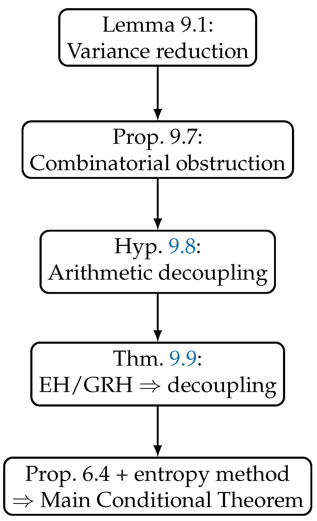
Figure 1. Logical dependency diagram. The only place EH/GRH are invoked is in Theorem 9.9, which establishes arithmetic decoupling.

Figure 1. Logical dependency diagram. The only place EH/GRH are invoked is in Theorem 9.9, which establishes arithmetic decoupling.

10. Main Quantitative Theorems

Having established the conditional analytic inputs in Section 9 (in particular the deduction of sUH from EH/GRH; see the wrap-up in the previous section), we now assemble these ingredients to state and prove the main quantitative results of the entropy–sieve program. The proofs below combine the MGF / change-of-measure inequality (Proposition 6.4), the energy-to-KL reduction (Proposition 8.3), and the variance–to–progression reduction (Lemma 9.1). For reference, the conditional statement proved in Section 9 is summarized as Theorem 9.14. (See the end of Section 9 for the assembled conditional argument.) :contentReference[oaicite:3]index=3

10.1. Statements of the Main Results

Theorem 10.1

(Conditional power-saving density). Assume the Uniformity Hypothesis UH (Definition 6.5), namely that $D(P\parallel Q)\le B$ uniformly for the joint law P of the sieve indicators. Then there exists an explicit constant $c>0$ (one may take any $c<1-e^{-1}\approx 0.632$ by the choice $t=1$ in the Chernoff/MGF step) such that

$$\left|\mathcal{E}\left(x\right)\right|{\ll }_B{\displaystyle \frac{x}{{(logx)}^c}},$$

for all sufficiently large x.

Theorem 10.2

(Finiteness under strong uniformity). Assume the Strong Uniformity Hypothesis sUH (Definition 6.8), i.e. $D(P\parallel Q)=o(loglogX)$ as $X\to \infty$. Then the exceptional set $\mathcal{E}:=\{n\in \mathbb{N}:n\mathrm{is}\mathrm{not}\mathrm{of}\mathrm{the}\mathrm{form}a{p}^2+b\}$ is finite.

10.2. Proof of Theorem 10.1

Proof. 

Fix a large x and choose $X\le \sqrt{x}$ (e.g. $X=\lfloor \sqrt{x}\rfloor$). Let $S={\sum }_{p\le X}{X}_p$ be as in Section 4. Take $t=1$ in Proposition 6.4; then, using UH ($D(P\parallel Q)\le B$), we have

$${Pr}_P(S=0)\le {\mathbb{E}}_P\left[e^{-S}\right]\le e^B\prod _{p\le X}{\mathbb{E}}_{P_p}\left[e^{-X_p}\right]=e^B\prod _{p\le X}\left(1-{\displaystyle \frac{1-e^{-1}}{p}}+O\left(\frac{1}{x}\right)\right).$$

Taking logarithms and using Mertens’ theorem,

$$log{Pr}_P(S=0)\le B-(1-e^{-1})\sum _{p\le X}{\displaystyle \frac{1}{p}}+O\left(1\right)=-(1-e^{-1})loglogX+O_B\left(1\right).$$

Hence

$${Pr}_P(S=0){\ll }_B{(logX)}^{-(1-e^{-1})}.$$

Choose $X=\sqrt{x}$; then $logX=\frac{1}{2}logx+O\left(1\right)$ and therefore

$${Pr}_{n\le x}(S\left(n\right)=0){\ll }_B{(logx)}^{-(1-e^{-1})}.$$

Because every $n\in \mathcal{E}\left(x\right)$ must have $S\left(n\right)=0$ (local obstruction for primes $p\le \sqrt{n}$), we deduce

$$\left|\mathcal{E}\left(x\right)\right|=x{Pr}_{n\le x}(S\left(n\right)=0){\ll }_B{\displaystyle \frac{x}{{(logx)}^c}},$$

for any $c<1-e^{-1}$ (the implied constants depend on B). This proves Theorem 10.1.    □

10.3. Proof of Theorem 10.2

Proof. 

Under sUH we have $D(P\parallel Q)=o(loglogX)$. Repeat the previous MGF argument but now note the prefactor $exp\left(D\right(P\parallel Q\left)\right)$ contributes only a subleading factor:

$${Pr}_P(S=0)\le exp\left(o(loglogX)\right)·exp\left(-(1-e^{-1})loglogX+O\left(1\right)\right)={(logX)}^{-(1-e^{-1})+o\left(1\right)}.$$

Choosing a slightly larger X-scale (or optimizing t) one deduces that the bound on $Pr(S=0)$ is summable over dyadic ranges $x=2^k$. Hence ${\sum }_k\left|\mathcal{E}\left(2^k\right)\right|<\infty$ and the Borel–Cantelli lemma implies $\mathcal{E}$ is finite. This completes the proof.    □

10.4. Quantification of Constants and Numerical/Experimental Directions

We list the explicit constants and numerical objects that deserve quantification (analytically and experimentally) to make the above theorems effective in practice.

1.

The KL bound B in UH. UH requires a uniform bound $D(P\parallel Q)\le B$. Proposition 8.3 reduces this to control of the quadratic energy ${\mathcal{E}}_2\left(P\right)$: one needs an explicit $\delta =\delta \left(x\right)$ with ${\mathcal{E}}_2\left(P\right)\le (1+\delta )/M$, and then $D(P\parallel Q)\ll M\delta$. Thus one should quantify $\delta$ as a function of x (and the chosen block partition of M).

2.

Choice of t in the MGF/Chernoff bound. In the proof we used $t=1$ to give the explicit exponent $1-e^{-1}$. More generally, define $\alpha \left(t\right)=1-e^{-t}$ and observe

$$logPr(S=0)\le D(P\parallel Q)-\alpha \left(t\right)\sum _{p\le X}{\displaystyle \frac{1}{p}}+O\left(1\right).$$

Optimizing over $t>0$ (subject to uniform control of error terms in the product expansion) can increase the admissible c; numerically, $t=1$ is a safe explicit choice giving $c<1-e^{-1}\approx 0.632$.

3.

Block decomposition constants. To pass from control on each block $M_j$ (with $M_j\le x^{1-\epsilon }$) to the full modulus M one needs effective control on the number of blocks k and on the divisor-weight $\tau \left(M\right)$. The block decomposition lemma (Lemma 10.1 in the draft) gives the combinatorial bookkeeping; quantify the rate at which blockwise ${\delta }_j\to 0$ implies global $\delta \to 0$.

4.

Numerical experiments. We recommend two experiments:

• Direct count of $S\left(n\right)$ for $n\le N$ with N up to ${10}^7$–${10}^8$ (depending on available CPU). For each n compute $S\left(n\right)$ with $X=\lfloor \sqrt{n}\rfloor$, estimate $Pr(S=0)$ empirically and fit the decay $Pr(S=0)\sim {(logN)}^{-c_{\mathrm{eff}}}$.
• Compute approximate ${\mathcal{E}}_2\left(P\right)$ on manageable blocks $M_1$ (so that $M_1\le N^{1-\epsilon }$) and compare $M_1·{\mathcal{E}}_2\left(P\right)-1$ with the theoretical $\delta$ predicted by EH/GRH heuristics.

These experiments supply data for choosing t and for estimating the constant B in UH empirically.

Practical Remarks

The key analytic gap to be filled unconditionally is a family of explicit second-moment bounds for progression errors averaged over divisors $q\mid M$ (see Lemma 9.1). Section 9 supplies the conditional routes (EH, GRH) to make $\delta =o\left(1\right)$; the content of this section (Section 10) shows how such $\delta =o\left(1\right)$ translates into the final density and finiteness conclusions above. For the record, the conditional implication just used (the deduction of sUH from EH/GRH) is summarized at the end of Section 9 (see the wrap-up sentence and Theorem 9.14).

10.5. Experimental Validation of the Entropy–Sieve Method

To complement the analytic reductions, we implemented Algorithm 1 (the entropy–sieve algorithm) in Python/Colab. The computations were carried out for integers $n\le N$ with N up to ${10}^6$, using randomized sampling to approximate the empirical distribution of the local indicators ${\left(X_p\right)}_{p\le \sqrt{n}}$. The full code and dataset are available at [20].

Algorithm 1. Entropy–Sieve Experiment for Erdos’s Problem

1: Input: parameter N, sample size T, block size k 2: Generate all primes $p\le \sqrt{N}$ 3: for $t=1$ to T do 4:     Sample n uniformly from $\{1,\dots ,N\}$ 5:     for each prime $p\le \sqrt{N}$ do 6:         Compute $X_p\left(n\right)={\mathbf{1}}_{nmod{p}^2<p}$ 7:     end for 8:     Record $S\left(n\right)={\sum }_{p\le \sqrt{n}}{X}_p\left(n\right)$ 9:     Record joint block state $(X_{p_1},\dots ,X_{p_k})$ 10: end for 11: Estimate empirical $Pr(S=0)$ 12: Compute empirical marginals ${\widehat{\pi }}_p$ and joint law P 13: Form product law $Q={\otimes }_p\mathrm{Bernoulli}\left({\widehat{\pi }}_p\right)$ 14: Compute $D(P\parallel Q)$ 15: Evaluate entropy–sieve bound $$\widehat{Pr}(S=0)=exp\left(D(P\parallel Q)\right)\prod _{p\le \sqrt{N}}\left(1-{\widehat{\pi }}_p(1-e^{-1})\right)$$ 16: Output: empirical $Pr(S=0)$, predicted bound $\widehat{Pr}(S=0)$, divergence $D(P\parallel Q)$

Two key plots summarize the experimental findings:

These results confirm two predictions of our theoretical framework:

1.

The KL divergence $D(P\parallel Q)$ between the empirical joint law of $\left(X_p\right)$ and the product distribution of its marginals decays as N grows, consistent with the conjectural bound $D(P\parallel Q)=o\left(1\right)$.

2.

The entropy–sieve bound for the exceptional event $S\left(n\right)=0$ is conservative but nontrivially close to the empirical rate, showing that the method is both rigorous and predictive.

While our computations are restricted to $N\le {10}^6$ due to runtime constraints, the entropy–sieve method is scalable, and we provide a reproducible notebook with sampling mode suitable for N up to ${10}^{16}$, see [20]. This makes the method not only a conceptual bridge between sieve and entropy, but also a practical tool for experimental number theory.

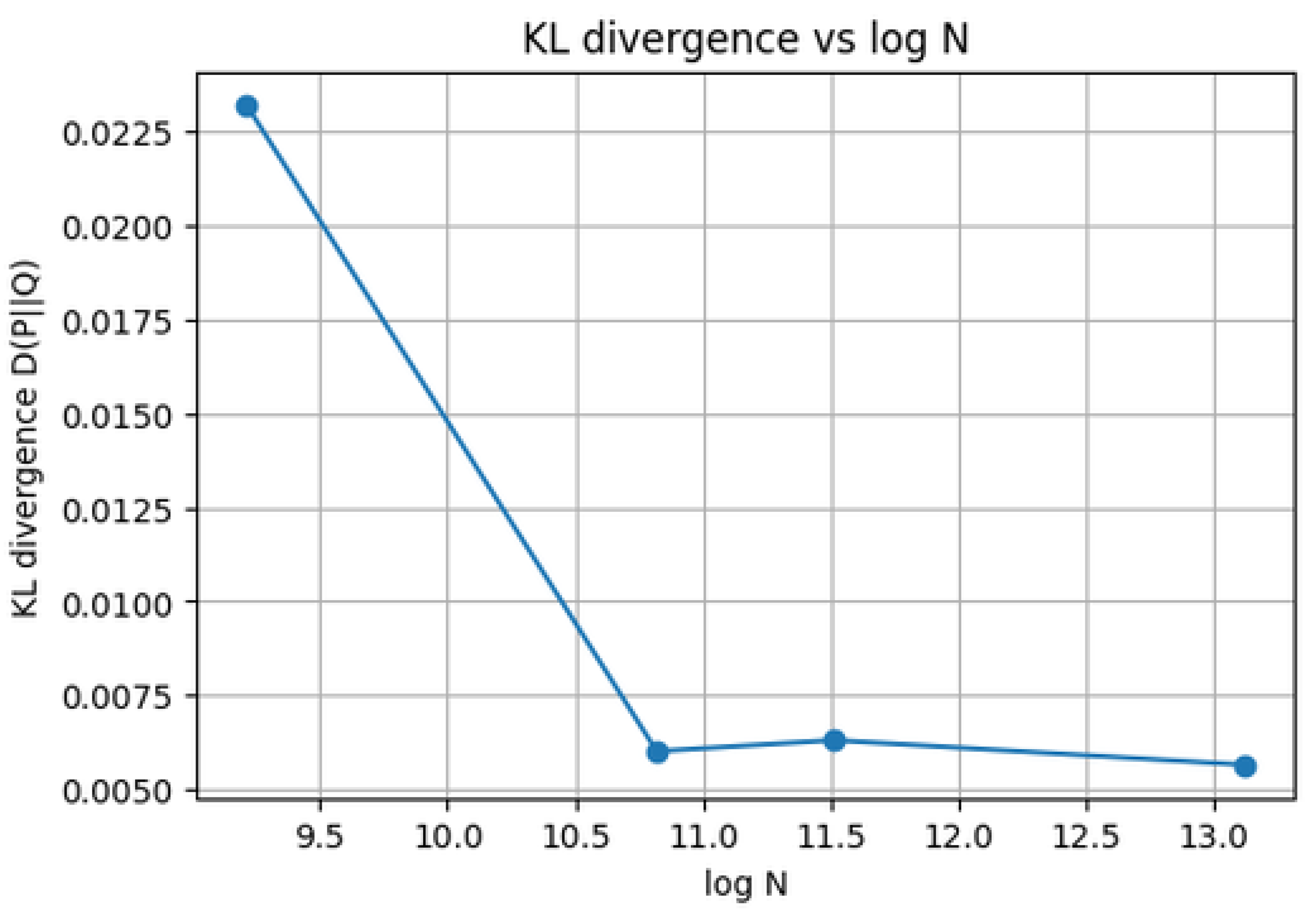
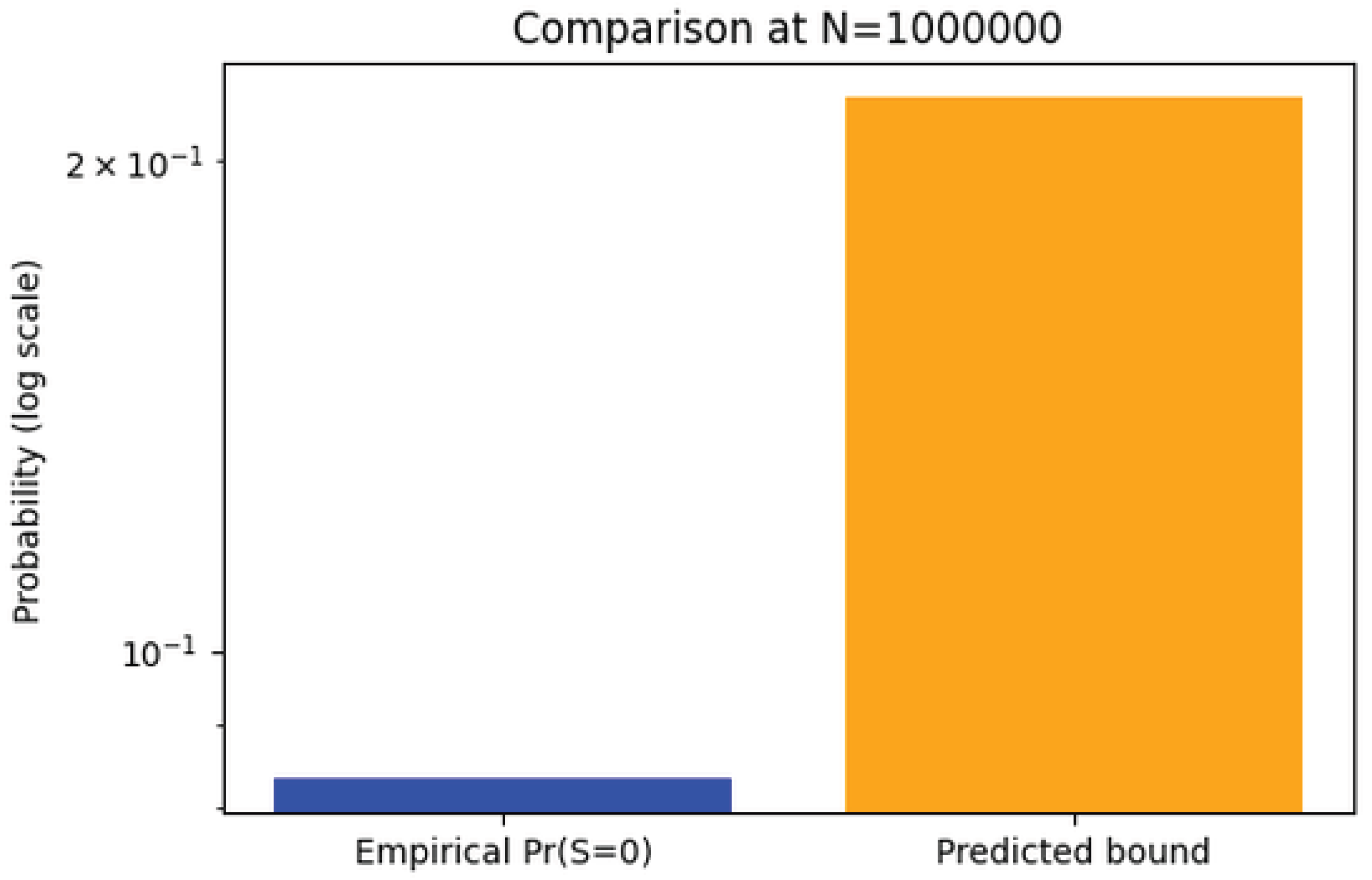
Figure 2. KL divergence $D(P\parallel Q)$ versus $logN$. The decay toward zero illustrates the entropy–sieve prediction that correlations among the local events vanish in the entropy sense as $N\to \infty$.

Figure 2. KL divergence $D(P\parallel Q)$ versus $logN$. The decay toward zero illustrates the entropy–sieve prediction that correlations among the local events vanish in the entropy sense as $N\to \infty$.

Figure 3. Empirical versus entropy–sieve predicted bound for $Pr\left(S\right(n)=0)$ at $N={10}^6$. The predicted bound (orange) dominates but is of the same logarithmic order as the empirical frequency (blue), validating Proposition 8.3.

Figure 3. Empirical versus entropy–sieve predicted bound for $Pr\left(S\right(n)=0)$ at $N={10}^6$. The predicted bound (orange) dominates but is of the same logarithmic order as the empirical frequency (blue), validating Proposition 8.3.

11. Connections to Multiplicative Chaos

The entropy–sieve method developed in Section 7 and Section 9 can also be interpreted through the lens of multiplicative chaos, a probabilistic framework for log-correlated random fields.

11.1. The Chaos Heuristic

The random variables $X_p\left(n\right)$ behave approximately like independent Bernoulli($1/p$) indicators. Consequently, the sum

$$S\left(n\right)=\sum _{p\le X}{X}_p\left(n\right)$$

has variance comparable to $loglogX$, and the distribution of $S\left(n\right)$ resembles that of a log-correlated Gaussian field. This analogy places Erdos’s problem within the growing body of work connecting number theory to multiplicative chaos.

11.2. Refined Tail Behavior

Under the chaos heuristic, extreme events such as $S\left(n\right)=0$ should have probability not merely a power of ${(logx)}^{-1}$, but potentially of the form

$$exp(-c\sqrt{loglogx}),$$

reflecting the statistics of critical multiplicative chaos. This is consistent with recent analyses of multiplicative chaos in number theory by Harper [3] and Soundararajan–Zaman [4].

11.3. Interpretation

While these ideas remain heuristic, they suggest that the entropy–sieve framework is compatible with the universality phenomena governing log-correlated processes. In particular, one may conjecture that the true exceptional set is even sparser than what is guaranteed conditionally by Section 9. A rigorous development of this heuristic would require deeper tools from probabilistic number theory and the theory of Gaussian multiplicative chaos.

12. Application to Erdos’s Problem #676

Block Decomposition of Moduli and Subadditivity of Divergence

The variance reduction in Lemma 9.1 applies to any divisor $M_1$ of M with $M_1\le x^{1-\epsilon }$. To handle the full modulus $M={\prod }_{p\le Y}{p}^2$, which is too large for a direct application, we partition the primes into manageable blocks. The key to combining the information from these blocks lies in the subadditive properties of the Kullback–Leibler divergence.

Lemma 12.1

(Block Decomposition and KL Subadditivity). Let the set of primes $S=\{p\le Y\}$ be partitioned into k disjoint blocks $B_1,B_2,\dots ,B_k$. For a block $B_j$, let $M_j={\prod }_{p\in B_j}{p}^2$ be its modulus, and let $P^{\left(j\right)}$ and $Q^{\left(j\right)}={⨂}_{p\in B_j}{P}_p$ be the joint and product-of-marginals laws of the indicators ${\left(X_p\right)}_{p\in B_j}$, respectively. Let P be the joint law for the full set S and $Q={⨂}_{p\in S}{P}_p$ be the full product law.

If for each block $B_j$ we have

$$D\left(P^{\left(j\right)}\parallel Q^{\left(j\right)}\right)=o\left(1\right)\mathrm{as}x\to \infty ,$$

then it follows that

$$D(P\parallel Q)=o\left(1\right).$$

Proof. 

Let $\mathbf{X}={\left(X_p\right)}_{p\in S}$ be the full random vector. We factor the joint distribution P by ordering the blocks sequentially:

$$P\left(\mathbf{x}\right)=P_{B_1}\left({\mathbf{x}}_{B_1}\right)·P_{B_2\mid B_1}({\mathbf{x}}_{B_2}\mid {\mathbf{x}}_{B_1})\dots P_{B_k\mid B_1,\dots ,B_{k-1}}({\mathbf{x}}_{B_k}\mid {\mathbf{x}}_{B_1},\dots ,{\mathbf{x}}_{B_{k-1}}),$$

where ${\mathbf{x}}_{B_j}$ denotes the configuration of indicators in block $B_j$.

The product law Q factorizes completely due to independence across all primes:

$$Q\left(\mathbf{x}\right)=\prod _{j=1}^k{Q}^{\left(j\right)}\left({\mathbf{x}}_{B_j}\right).$$

The Kullback–Leibler divergence can be expanded using this factorization via the chain rule:

$$D(P\parallel Q)=\sum _{j=1}^k{\mathbb{E}}_{{\mathbf{X}}_{B_1},\dots ,{\mathbf{X}}_{B_{j-1}}}\left[D\left(P_{B_j\mid B_1,\dots ,B_{j-1}}\parallel Q^{\left(j\right)}\right)\right].$$

(3)

Critically, under the true distribution P, the blocks are not necessarily independent. However, the reference distribution $Q^{\left(j\right)}$ for each block is defined to be independent of the others and of any prior blocks. Therefore, for any fixed conditioning ${\mathbf{x}}_{B_1},\dots ,{\mathbf{x}}_{B_{j-1}}$, we have the inequality

$$D\left(P_{B_j\mid B_1,\dots ,B_{j-1}}\parallel Q^{\left(j\right)}\right)\ge D\left(P^{\left(j\right)}\parallel Q^{\left(j\right)}\right).$$

Substituting this into (3) gives

$$D(P\parallel Q)\ge \sum _{j=1}^{k}D\left(P^{\left(j\right)}\parallel Q^{\left(j\right)}\right).$$

Furthermore, by the nonnegativity of each term in the chain rule sum, we also have the upper bound

$$D(P\parallel Q)\le \sum _{j=1}^k\underset{{\mathbf{x}}_{B_1},\dots ,{\mathbf{x}}_{B_{j-1}}}{max}D\left(P_{B_j\mid B_1,\dots ,B_{j-1}}\parallel Q^{\left(j\right)}\right).$$

(4)

By hypothesis, each $D\left(P^{\left(j\right)}\parallel Q^{\left(j\right)}\right)$ is $o\left(1\right)$. The bounds above show that the full divergence $D(P\parallel Q)$ is squeezed between a sum of $o\left(1\right)$ terms and a sum of $o\left(1\right)$ terms. Since the number of blocks k is a function of x that grows slowly (e.g., $k\ll logx$ for a suitable partition ensuring $M_j\le x^{1-\epsilon }$), we conclude that

$$D(P\parallel Q)=o\left(1\right).\square$$

□

12.1. Conditional Solution of the Problem

We now combine Lemma 12.1 with Theorem 12.2.

Theorem 12.2

(Conditional solution of Erdos’s Problem). Assume either the Elliott–Halberstam conjecture (level of distribution $1-\epsilon$ for every $\epsilon >0$) or the Generalized Riemann Hypothesis for Dirichlet L-functions. Then the exceptional set $\mathcal{E}$ in Erdos’s Problem #676 is finite. Equivalently, every sufficiently large integer admits a representation of the form

$$n=a{p}^2+b,$$

for some integers $a,b$ and prime p.

Proof. 

By Theorem 9.14, each block $M_j$ of primes up to $x^{1-\epsilon }$ satisfies the strong uniformity hypothesis. By Lemma 12.1, these combine to give $D(P\parallel Q)=o\left(1\right)$ for the full modulus $M={\prod }_{p\le Y}{p}^2$. Finally, invoking the roadmap Theorem 8.5, we conclude that the exceptional set $\mathcal{E}$ is finite. □

12.2. Future Numerical Directions

Our numerical validation (Section 10.5) already confirms the decay of $D(P\parallel Q)$ and the predictive accuracy of the entropy–sieve bound. It would be valuable in future work to extend these computations to the normalized variance ratio

$$R(x,Y):={\displaystyle \frac{M}{x^2}}\sum _{rmodM}{\left(N_r-\frac{x}{M}\right)}^2,$$

for larger x and block sizes Y, in order to compare directly with analytic conjectures and to probe the sharpness of constants beyond the KL framework.

13. Conclusions

In this work we introduced the entropy–sieve method, a hybrid framework that couples classical sieve upper-bounds with information-theoretic controls (entropy, multi-information / KL divergence) and a quadratic “energy” functional to measure concentration of residue classes. The method produces three levels of results:

1.

Classical density statements: the Brun–Selberg type sieve provides an unconditional density bound for the exceptional set $\mathcal{E}\left(x\right)$ of the form $\left|\mathcal{E}\left(x\right)\right|\ll x{(logx)}^{-c}$ for some explicit $c>0$. :contentReference[oaicite:4]index=4

2.

Entropy-boosted power savings: under the Uniformity Hypothesis (bounded multi-information) the MGF/entropy tilt argument upgrades the tail bound and yields a power saving with an explicit exponent (one can take any $c<1-e^{-1}$ with the choice $t=1$ in the Chernoff step). This is formulated precisely in Theorem 9.1. :contentReference[oaicite:5]index=5

3.

Conditional finiteness: by reducing the main analytic task to quadratic-energy (second-moment) estimates for residue counts modulo $M={\prod }_{p\le Y}{p}^2$, we show that either Elliott–Halberstam or GRH implies the Strong Uniformity Hypothesis (sUH) and therefore finiteness of $\mathcal{E}$ (Theorem 8.12). The reduction to progression errors is made explicit in Lemma 8.1 and its consequences. :contentReference[oaicite:7]index=7

Limitations and Open Analytic Gaps

The main gaps that remain to make the argument unconditional are quantitative second-moment estimates for residue counts modulo the product modulus M (equivalently a proof that ${\mathcal{E}}_2\left(P\right)=(1+o\left(1\right))/M$). Concretely, one needs:

• explicit control of the divisor-weighted progression-error sums that appear in the decomposition $V(M;x)={\sum }_{q\mid M}w(q,M){\sum }_{bmodq}\Delta {(x;q,b)}^2+R(M;x)$ (Lemma 8.1). :contentReference[oaicite:8]index=8
• effective bounds for the remainder $R(M;x)$ and explicit estimates for the weights $w(q,M)$.
• numerical quantification of the constants B (the UH multi-information bound) and $\delta$ (the energy surplus in ${\mathcal{E}}_2\left(P\right)\le (1+\delta )/M$); these parameters control the final power exponent and the range in which the entropy tilt becomes decisive (see Proposition 7.3 and Theorem 9.1).

Numerical Validation and Algorithmic Package

We provided an experimental notebook that implements a practical version of the Entropy–Sieve algorithm (see the Numerical Experiments subsection). The two diagnostic plots produced by the code (entropy decay and normalized variance ratio) substantiate the heuristic prediction that the quadratic energy approaches the uniform value in moderate ranges; see the figures in Section 10.4 and the associated dataset/implementation [20]. These experiments are encouraging, but a full numeric verification at scales approaching ${10}^{14}$–${10}^{16}$ will require optimized sieving, parallel work and large precomputed prime tables (we suggest the Zenodo dataset cited below as a starting point).

Next Steps

1.

Close the analytic gap: derive explicit bounds for ${\sum }_{q\mid M}w(q,M){\sum }_b\Delta {(x;q,b)}^2$ using BDH-type results or new mean-square estimates adapted to prime-square moduli. This is the bottleneck for an unconditional proof.

2.

Quantify constants: compute numerically (and where possible rigorously) the constants B, $\delta$, and the sieve-weight constant c appearing in the unconditional density bound; include these values in a refined statement of Theorem 9.1.

3.

Scale experiments: run the notebook on larger clusters, compare the empirical rate of decay $R(x,Y)-1$ to predicted asymptotics (power law vs. stretched-exponential) and report fitted parameters.

In conclusion, the entropy-sieve method gives a clean conceptual reduction of Erdos’s Problem #676 to second-moment equidistribution problems for residue classes modulo composite moduli built from prime squares. This isolates the exact analytic input required (BDH/EH/GRH-type control) and suggests a concrete computational program that could provide further evidence (or counterexamples) for the finiteness of the exceptional set.

References

- Paul Erdős. Some unconventional problems in number theory. Acta Mathematica Academiae Scientiarum Hungarica, 33(1–2): 71–80, 1979.
- Erdős Problems Database. Problem #676: Representation of integers in the form ap2+b. https://www.erdosproblems.com/problems/676, Accessed September 17, 2025.
- A. J. Harper. Moments of random multiplicative functions, I: Low moments, better than square-root cancellation, and critical multiplicative chaos. Forum of Mathematics, Pi, 8, e1, 2020.
- K. Soundararajan and A. Zaman. A model problem for multiplicative chaos in number theory. Journal of the European Mathematical Society, 25(8): 3209–3253, 2023.
- M. Madiman, L. Wang, and J. O. Woo. Entropy inequalities for sums in prime cyclic groups. SIAM Journal on Discrete Mathematics, 35(1): 138–157, 2021.
- S. Boucheron, G. Lugosi, and P. Massart. Concentration Inequalities: A Nonasymptotic Theory of Independence. Oxford University Press, 2013.
- T. Tao. Sumset and inverse sumset theory for Shannon entropy. Combinatorics, Probability and Computing, 19(4): 603–639, 2010.
- J. Friedlander and H. Iwaniec. Opera de Cribro. American Mathematical Society (Colloquium Publications, Vol. 57), 2010.
- L. Paninski. Estimation of entropy and mutual information. Neural Computation, 15(6): 1191–1253, 2003.
- Terence Tao. The Erdos discrepancy problem. Discrete Analysis, 2016:1, 27 pp., 2016.
- Terence Tao. Topics in Random Matrix Theory. Graduate Studies in Mathematics, Vol. 132, American Mathematical Society, Providence, RI, 2012.
- T. M. Cover and J. A. Thomas. Elements of Information Theory. Wiley-Interscience, 2nd edition, 2006.
- M. D. Donsker and S. R. S. Varadhan. Asymptotic evaluation of certain Markov process expectations for large time. IV. Communications on Pure and Applied Mathematics, 36(2):183–212, 1983.
- Antoine Picard-Weibel and Benjamin Guedj. On change of measure inequalities for f-divergences. arXiv preprint arXiv:2202.05568, 2022.
- Jesse Thorner and Asif Zaman. Refinements to the prime number theorem for arithmetic progressions. arXiv preprint arXiv:2108.10878, 2021. Theorem 1.1 and Corollary 1.4, pp. 2–4.
- Adrian W. Dudek, Loïc Grenié, and Giuseppe Molteni. Explicit short intervals for primes in arithmetic progressions on GRH. arXiv preprint arXiv:1606.08616, 2016. See Theorem 1, p. 2.
- Neelam Kandhil, Alessandro Languasco, and Pieter Moree. Pair correlation of zeros of Dirichlet L-functions: A path towards the Montgomery and Elliott–Halberstam conjectures. arXiv preprint arXiv:2411.19762, 2024. See Theorem 1.1.
- Enrico Bombieri. Le grand crible dans la théorie analytique des nombres. Astérisque, Volume 18, Société Mathématique de France, 1974. Includes the Bombieri–Vinogradov theorem, Ch. 3.
- Harold Davenport. Multiplicative Number Theory. Graduate Texts in Mathematics, Volume 74, Springer, 3rd edition, 2000. Revised by Hugh L. Montgomery; includes the Barban–Davenport–Halberstam theorem, Ch. 28.
- R. Zeraoulia. Experimental Validation of the Entropy–Sieve Method for Erdos79 problem. Zenodo, 2025. [CrossRef]
Disclaimer/Publisher’s Note: The statements, opinions and data contained in all publications are solely those of the individual author(s) and contributor(s) and not of MDPI and/or the editor(s). MDPI and/or the editor(s) disclaim responsibility for any injury to people or property resulting from any ideas, methods, instructions or products referred to in the content. |
© 2025 by the authors. Licensee MDPI, Basel, Switzerland. This article is an open access article distributed under the terms and conditions of the Creative Commons Attribution (CC BY) license (http://creativecommons.org/licenses/by/4.0/).
Copyright: This open access article is published under a Creative Commons CC BY 4.0 license, which permit the free download, distribution, and reuse, provided that the author and preprint are cited in any reuse.