Submitted:
02 September 2025
Posted:
03 September 2025
You are already at the latest version
Abstract
This study investigates the structural dynamics of consumer prices in Japan by analyzing monthly Consumer Price Index (CPI) data for ten major categories from January 1970 to December 2024. Each category's CPI is decomposed into trend, seasonal, and cyclical components using an integrated moving linear model approach that simultaneously performs seasonal adjustment and trend-cycle decomposition. Unlike conventional methods, this approach enables the concurrent estimation of trend and seasonal components while iteratively extracting cyclical fluctuations, without imposing restrictive probabilistic assumptions. The resulting components reveal time-varying features such as shifts in seasonality, changes in trend growth rates, and variations in cyclical amplitudes. By further examining interrelationships among categories, the analysis uncovers structural changes, divergence and convergence patterns, and evolving linkages with macroeconomic conditions. Beyond offering a comprehensive understanding of the Japanese CPI fluctuations, this study demonstrates a methodological framework that can be applied to other economies for analyzing long-term structural transformations and short-term dynamics. Our findings provide insights relevant to inflation monitoring, macroeconomic stability, and the broader literature on structural change and economic dynamics.
Keywords:
moving linear model approach
; economic time series
; components decomposition
; dynamic structure
; category’s CPI
1. Introduction
Understanding the structural dynamics of consumer prices is essential for assessing inflationary trends, identifying phases of business cycles, and formulating effective macroeconomic policies.1 In Japan, the Consumer Price Index (CPI) serves as a primary indicator for measuring price stability and guiding monetary policy decisions. However, aggregate CPI figures often conceal substantial heterogeneity across sectors, making it challenging to capture sector-specific price behaviors and their respective contributions to overall inflation (Blinder, 1982; Bryan and Cecchetti, 1993; Hale and Jorda, 2007).
This study addresses this issue by analyzing monthly CPI data for Japan disaggregated into ten major categories over the period from January 1970 to December 2024. While each category’s CPI exhibits complex behavior, it can broadly be modeled as comprising three primary components: a long-term trend, seasonal fluctuations, and cyclical variations (Harvey, 1990; Baxter and King, 1999). By decomposing each category’s CPI into these components, it becomes possible to extract and interpret the underlying patterns of variation more effectively.
To achieve this decomposition, we employ the integrated moving linear (ML) model approach developed by Kyo and Kitagawa (2023) and extended by Kyo et al. (2024). This unified framework enables simultaneous seasonal adjustment and trend-cycle decomposition, offering flexibility in modeling the components without imposing rigid assumptions on their probabilistic properties. Such flexibility enhances both the robustness and interpretability of the results, which is particularly important for long time series subject to structural changes (Stock and Watson, 2016).
The analysis proceeds in two stages. First, each category’s CPI time series is decomposed into its trend, seasonal, and cyclical components. Second, the statistical properties and variation patterns of each component are examined, followed by a comparative and integrative assessment across all categories to identify interrelationships and structural changes in the CPIs over the past five decades. Special attention is given to shifts in cyclical behavior, modifications in seasonal patterns, and long-term divergence or convergence among categories.
The findings of this study are expected to provide new insights into the mechanisms shaping CPI dynamics in Japan. From a policy perspective, they offer valuable implications for inflation monitoring, the design of monetary and fiscal measures, and the understanding of sector-specific drivers of both short- and long-term price movements. To the best of our knowledge, no other research exists with content similar to that of this study.
The remainder of the article is organized as follows. Section 2 outlines the study’s objectives and contributions. Section 3 introduces the employed methodology. Section 4 presents the results of the component decomposition for each category’s CPI time series and describes the additional analyses. Section 5 concludes the article.
2. Objectives and Contributions
The primary objective of this study is to uncover the structural characteristics and long-term changes in Japan’s consumer price system by decomposing and analyzing monthly CPI data for ten major categories over the period 1970–2024. Specifically, our study pursues the following objectives.
- Decompose each category’s CPI into trend, seasonal, and cyclical components using an integrated ML model approach.
- Characterize the temporal behavior of each component, including changes in the amplitude and persistence of cyclical variations, shifts in seasonal patterns, and gradual or abrupt changes in trend growth rates.
- Compare and synthesize the results across all categories to detect interrelationships and structural shifts in the consumer price system, including divergence/convergence among categories and sector-specific inflation patterns.
- Provide empirical evidence on the evolution of Japan’s inflation dynamics, highlighting sectoral contributions to aggregate CPI movements and their linkages with macroeconomic conditions.
This study makes several contributions to the related literature. First, it offers a long-term, high-frequency component analysis of CPI across ten categories, a perspective often overlooked in aggregate inflation research. Second, by applying the integrated ML model approach, it achieves more precise extraction of seasonal and cyclical components than conventional methods, thereby enhancing both interpretability and robustness. Third, its comparative framework across categories provides a nuanced understanding of structural changes in Japan’s price system, with implications for inflation monitoring, monetary policy, and sectoral economic analysis.
3. Methodology
This section outlines the methodology used to decompose the monthly time series data of Japan’s CPI for each of the ten categories into trend, seasonal, and cyclical components. The employed approach is the integrated ML model method of Kyo et al. (2024), developed on the basis of the ML model approach originally proposed by Kyo and Kitagawa (2023).
3.1. Basic Framework
Let denote the monthly time series for each category’s CPI. We consider the model
where N is the length of the time series. Additionally, and represent the trend and cyclical components, respectively. In Kyo and Kitagawa (2023), these components are treated more generally and referred to as the constrained component and the remaining component, respectively.
Furthermore, the trend is assumed to be smoothed over time. To ensure smoothness within each local time interval, it is represented using a linear model in time. For this purpose, we introduce an integer parameter k, which denotes the width of the time interval (WTI).
Specifically, for a time interval with , we adopt the linear model
where and are coefficients. The model in Eq. (2) is referred to as the local linear model, since and remain constant for a fixed n but can vary across different intervals.
The time points can be expressed as
where is the midpoint of the interval. Substituting this expression for t into Eq. (2) yields
where the values of for are independent of n and have an average of zero. Therefore, represents the average of over the interval.
Using Eq. (3), the model in Eq. (1) can be rewritten as
To reliably estimate the trend and cyclical components, the parameters , , for are treated as random variables, and a set of probabilistic constraints is imposed on them. In this way, the model can be expressed in state-space form, and the parameters can be estimated using the Kalman filter algorithm.
Once the estimates of the cyclical component are obtained, the corresponding trend estimates can be calculated as
In Kyo and Kitagawa (2023), this method for decomposing a time series into trend and cyclical components is referred to as the moving linear (ML) model approach. In this framework, the trend captures the smoothed, time-varying mean of the series, while the remaining short-term fluctuations are absorbed by the cyclical component. An important aspect of the ML approach is the estimation method for k (the WTI), the details of which are given in Kyo (2025).
A distinctive feature of the ML approach is that, aside from the assumption that the cyclical component is approximately mean-stationary in the long run, no strict assumptions are imposed on it. This flexibility enables the approach to be applied to a wide range of contexts.
The present study, however, aims to extract the seasonal component as a distinct element, accounting for seasonal fluctuations and performing seasonal adjustment. In such cases, the ML model approach cannot be applied directly. Therefore, we adopt an extended ML approach, as described below, which builds on the method proposed in Kyo et al. (2024) and extends the decomposition framework to explicitly incorporate the seasonal component.
3.2. Extended ML Approach for Seasonal Adjustment
Assuming that the time series contains, in addition to the trend and cyclical component , a seasonal component , we introduce the model
which can be considered as an extended form of the model in Eq. (1).
We focus on explaining the seasonal component below. In a time series, the seasonal component mainly consists of patterned variations that repeat every year. For monthly time series data, the period length p is typically set to 12. One characteristic of the seasonal component is that is approximately equal to , i.e.,
It follows that a sequence
arranged based on the time series of (), may exhibit high smoothness for appropriate integers j and m, and therefore behave similarly to a trend component.
Assuming that we have m years of monthly time series data, so that , the dataset can be divided into p subsets:
For a fixed j, the time series data in Eq. (6) can be regarded as a set of annual time series data, which can be represented as the sum of trend and cyclical components without the seasonal component. Accordingly, the model in Eq. (5) can be rewritten for these subsets as
If we define
then Eq. (7) can be expressed as
Based on the properties of the seasonal component, for a fixed j, can be treated as an extended trend, while can be regarded as the corresponding cyclical component within the ML model framework. Formally, Eq. (8) represents a trend-cyclical decomposition, and therefore the ML model approach can be applied to it.
3.3. Procedure for Component Decomposition
The time series can be decomposed into the trend , seasonal , and cyclical components through the following three-step procedure using the ML model approach.
Step 1: Extended Trend-Cyclical Decomposition. As shown in Eq. (9), for a fixed value of j, we regard and as the extended trend and cyclical components, respectively. We then decompose the annual time series into and . This decomposition is repeated p times, separately for . Using the decomposed results for with and , we can reconstruct a monthly time series as
Step 2: Seasonal Component Extraction. Based on the time series in Eq. (10), we construct the model
where and are regarded as the trend and seasonal components, respectively. The monthly time series is then decomposed into and using the ML model approach, and is taken as the final estimate of the seasonal component.
Note that a provisional estimate of the cyclical component has already been obtained in the previous step. However, since it was estimated separately for each j, it lacks consistency and needs to be re-estimated.
Step 3: Final Trend and Cyclical Decomposition. We first calculate the seasonally adjusted series
From the model in Eq. (5), the seasonally adjusted series can be represented as
and and are then decomposed into and using the ML model approach.
Consequently, the final estimates for the trend, seasonal, and cyclical components are , , and , respectively. As seen from this procedure, the seasonal and cyclical components are treated as remaining components in each step, highlighting the flexibility of the ML model approach. Inheriting the characteristics of the ML model, the Extended ML approach imposes minimal restrictions based on data distribution properties, making it widely applicable.
3.4. Estimating the Values of WTI for Each Step
In the second step of the component decomposition, the ML model approach is applied to the entire time series for each candidate value of , where is chosen appropriately according to the structure of the seasonal component. The value of k that maximizes the likelihood is then selected as its estimate. That is, the value of k can be estimated using the maximum likelihood method, as described in Kyo (2025).
It should be noted that if k exceeds a certain limit, part of the fluctuations in the cyclical component may be absorbed into the seasonal component, potentially disrupting the balance between the components. In such cases, it is advisable to review the estimation results and impose an appropriate restriction on k.
In the third step of the component decomposition, the decomposition is performed on the entire time series . Therefore, the value of k can also be estimated for using the same maximum likelihood method.
However, in the first step, the decomposition is applied to for and . Determining the value of k in this case is more challenging. Kyo et al. (2024) proposed a method that uses a common value of k across all . Under this method, the log-likelihood is evaluated for each j, and the average of these log-likelihoods is computed. The value of k is then chosen to maximize this average log-likelihood, yielding the estimate .
3.5. Advantages of the Approach
The extended ML model approach provides several benefits for CPI analysis as follows.
- Unified decomposition: Trend, seasonal, and cyclical components are estimated jointly within a coherent framework, avoiding potential distortions that may arise from sequential procedures.
- Flexibility: The method does not impose strict parametric assumptions on the cyclical component, allowing it to capture complex and time-varying cycle structures.
- Local adaptability: The WTI can be determined using the maximum likelihood method, and the resulting framework adapts to structural breaks and gradual changes in price dynamics.
- Computational efficiency: The state-space formulation combined with Kalman filtering enables scalable estimation for long monthly time series.
4. Results and Additional Analysis
In this section, we analyze monthly time series data for the major categories of Japan’s CPI. Each series is first decomposed into trend, seasonal, and cyclical components. We then examine the decomposed results to elucidate the characteristics of structural changes in Japan’s price system.
4.1. Data
The CPI in Japan is classified into ten major categories, as listed in Table 1.
The sample period spans January 1970 to December 2024, providing 660 monthly observations for each category. All data can be obtained from the Statistics Bureau of Japan (https://www.stat.go.jp/english/data/cpi/1581-z.html), with historical series linked to maintain continuity across changes in the CPI base year. The long time span allows us to capture both gradual structural changes and abrupt shifts associated with major macroeconomic events, such as the oil crises, financial bubbles, prolonged deflation, and the COVID-19 pandemic.
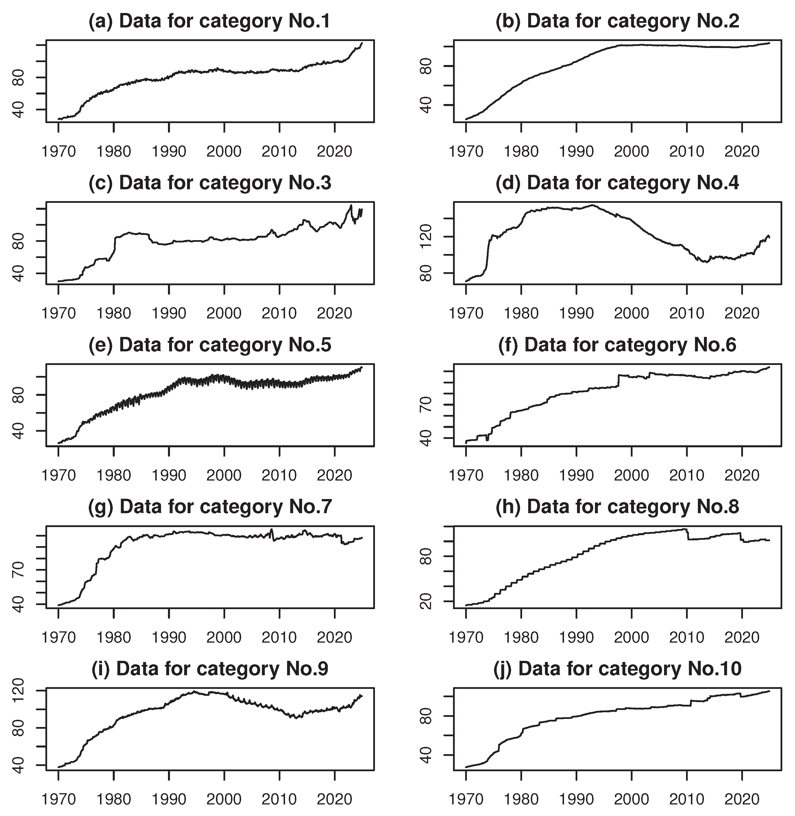
Line graphs of the CPI time series for each category are presented in Figure 5 of Appendix A. As shown in Figure 5, most categories exhibit sharp increases in the CPI during periods of rapid economic growth, followed by periods of stabilization.
4.2. Analysis of the Decomposition Results
Using the extended ML model approach described in Section 3.3, the monthly time series data for each CPI category were decomposed into trend, seasonal, and cyclical components. The results for each component are presented, followed by an analysis of the interrelationships among categories and the features of their behaviors.
4.2.1. Analysis of the Trend
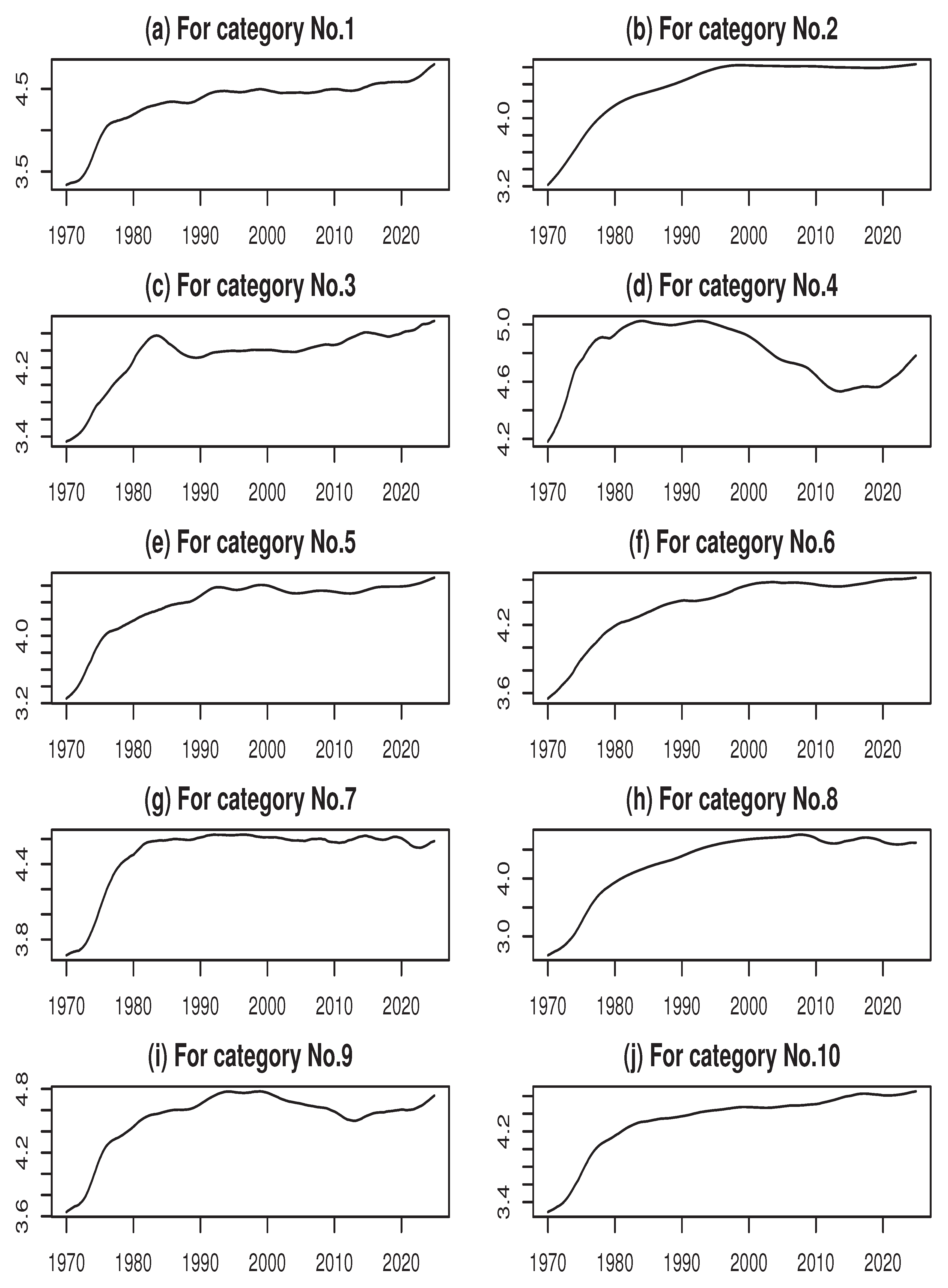
As a reference, the estimated trend components for each CPI category are shown in Figure 6 of Appendix B. These results illustrate the long-term fluctuations in each category’s CPI. A notable case is No. 4 (Furniture and Household Utensils), where the CPI peaked around the bursting of the bubble in 1992, declined until 2012, and has slightly increased in recent years. This trajectory reflects the decline in real estate prices following the bubble collapse.
To investigate trend fluctuations more closely, the differenced estimated trends are computed in Figure 1.
A common feature is evident: the differenced trends for nearly all categories peaked around late 1973, fell sharply, and then remained relatively stable. Some categories, however, exhibit distinctive movements. As for No. 3 (Fuel, Light, and Water Charges), the differenced trend showed a temporary plateau during the period of the early 1980s, likely due to rising demand associated with the housing boom. In No. 8 (Education), sharp declines appeared around 1999 and 2019, corresponding to the impacts of the domestic financial turmoil and the COVID-19 pandemic, respectively.2 Based on these trend patterns, the full sample period (January 1970 – December 2024) can be broadly divided into six phases.
-
Late High-Growth / Early Rising Phase (1970–1973):Gradual CPI increases driven by high growth and the 1971 shift to the floating exchange rate regime, followed by a sharp surge with the first oil shock in 1973.
-
Post Oil Shock Stabilization (1974–1985):After the steep 1974 rise, tighter policies and yen appreciation suppressed inflation and stabilized prices.3
-
Bubble Formation and Expansion (1986–1992):Yen depreciation after the Plaza Agreement and monetary easing fueled steady CPI increases during the economic boom.
-
Prolonged Deflation (1993–2012):Low growth and persistent price declines followed the bubble burst, with temporary spikes from the 1997 consumption tax hike.
-
Moderate Inflation (2013–2019):Yen depreciation and Abenomics policies lifted prices moderately, with temporary spikes from the 2014 and 2019 consumption tax hikes.
-
Global Inflation and Sharp Surge (2020–2024):An initial dip during early COVID-19 was followed by rapid increases, driven by soaring resource prices and yen depreciation after 2021.
To examine the similarity of trend fluctuations across categories, cluster analysis was applied to each phase. Ward’s method was used, with each variable standardized and centered within its period. The results are presented in Figure 2.
Our cluster analysis results as shown in Figure 2 provide interesting findings. First, overall, the similarities among the CPI categories are relatively low in Periods 2 and 4, which correspond to periods of significant structural change. Additionally, for each period, the relative similarities between certain CPI categories are as follows.
-
Period 1 (1970–1973):The strongest similarity between No. 3 (Fuel, Light, and Water Charges) and No. 10 (Miscellaneous) reflects their common dependence on imported resources and infrastructure costs. The pairing of No. 2 (Housing) and No. 4 (Furniture and Household Utensils) indicates the linkage between the housing market and durable consumer goods, driven by strong housing demand. The similarity between No. 7 (Transportation and Communication) and No. 9 (Culture and Recreation) corresponds to the simultaneous expansion of leisure and transport services during income growth.
-
Period 2 (1974–1985):The closest similarity between No. 1 (Food) and No. 2 (Housing) reflects stability in basic household expenditure categories. The pair No. 3 and No. 10 again shows a common pattern in resource-dependent costs. The similarity between No. 4 (Furniture) and No. 9 (Culture and Recreation) suggests a link between durable goods and leisure-related spending in the stable economic phase.
-
Period 3 (1986–1992):The cluster of No. 4 (Furniture), No. 5 (Clothing and Footwear), and No. 9 (Culture and Recreation) indicates synchronized price movements in durable goods, fashion, and leisure sectors, all benefiting from booming consumption. The similarity between No. 2 (Housing) and No. 7 (Transportation and Communication) reflects the simultaneous expansion of real estate prices and urban transport/communication infrastructure. The pairing of No. 8 (Education) and No. 10 (Miscellaneous) reflects rising demand for quality services during the expansion period.
-
Period 4 (1993–2012):The closest similarity between No. 5 (Clothing and Footwear) and No. 9 (Culture and Recreation) reflects intense price competition in these sectors. Equal similarities between No. 2 (Housing) and No. 10 (Miscellaneous), and between No. 3 (Fuel) and No. 7 (Transportation and Communication), suggest shared cost drivers. The similarity between No. 4 (Furniture) and No. 6 (Medical Care) may reflect changes in expenditure patterns under prolonged low-income growth.
-
Period 5 (2013–2019):The similarity between No. 3 (Fuel) and No. 10 (Miscellaneous) reflects the impact of yen depreciation on import prices. The pairing of No. 5 (Clothing and Footwear) and No. 9 (Culture and Recreation) indicates parallel demand increases in fashion and leisure sectors during economic recovery. No. 8 (Education) is closely linked to the No. 3 + No. 10 cluster, suggesting that education costs were also affected by import dependency and rising service costs.
-
Period 6 (2020–2024):The strongest similarity between No. 8 (Education) and No. 10 (Miscellaneous) reflects cost pass-through from rising wages and service expenses. The pairing of No. 4 (Furniture) and No. 5 (Clothing and Footwear) shows the shared impact of supply chain disruptions and rising import costs. The similarity between No. 1 (Food) and No. 2 (Housing) indicates that core household expenses became increasingly correlated, highlighting the pressure on living costs.
4.2.2. Analysis of the Seasonal Component
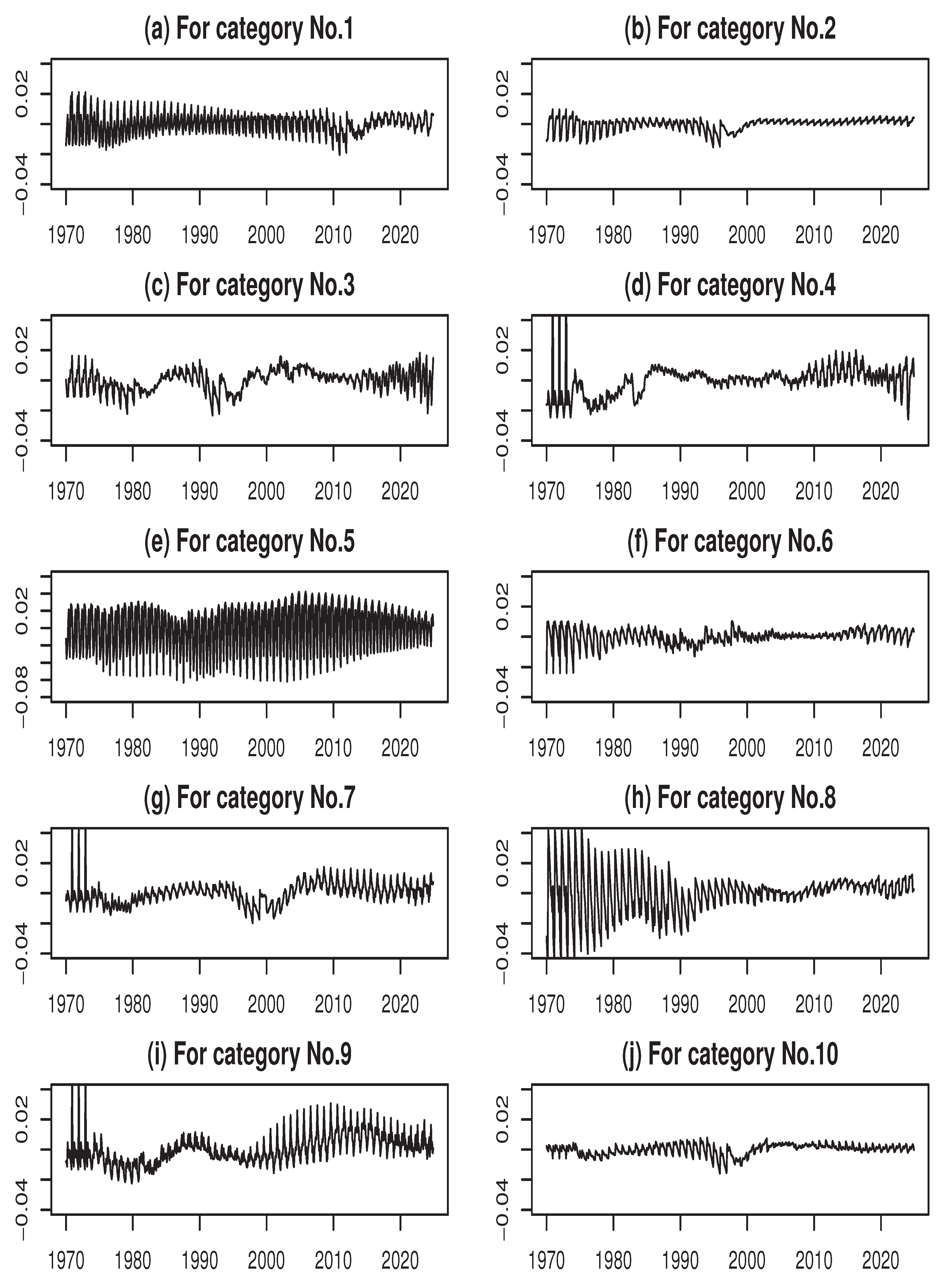
For reference, the estimated results of the seasonal components for each category are shown in Figure 7 of Appendix C. As is clearly observed in Figure 7, in category No. 5 (Clothing and Footwear), the seasonal fluctuations have become more pronounced along with the maturation of the economy, indicating the strong seasonality of product demand in this category.
Regarding the seasonal component, two types of variability can be identified. First, when viewed on a monthly basis, the variance of the twelve monthly values represents fluctuations around a mean of zero, which is referred to as amplitude variability. Second, the variability of the correlation coefficient between the twelve values in the current year and those in the twelve months of the previous year represents changes in the seasonal pattern, which is referred to as pattern variability. Figure 3 and Figure 4 show the amplitude variability and pattern variability for each category’s CPI.
From Figure 3, several observations can be made. First, as can also be observed in Figure 7, in many categories the amplitude variability of the seasonal component was extremely large during the period from 1970 to 1972. This is because the structure of the seasonal component underwent substantial changes around 1973. Therefore, Figure 3 has been constructed using data from May 1973 onward.
Next, in categories such as No. 2 (Housing), No. 3 (Fuel, Light, and Water Charges), and No. 10 (Miscellaneous), the amplitude variability increased during the early to mid-1990s. This can be interpreted as a reflection of the structural changes in the real estate industry following the collapse of the bubble economy. Furthermore, in categories such as No. 7 (Transportation and Communication) and No. 9 (Culture and Recreation), a rise in amplitude variability was observed somewhat later, from the late 1990s through around the end of the 2010s, likely due to the effects of informatization or digitalization in Japanese society.
Regarding pattern variability (Figure 4), values remain close to 1 at most points in time, indicating a generally high level of stability. Nevertheless, several noteworthy deviations can be observed. In No. 1 (Food), a sharp drop occurred in 2012, suggesting that the price fluctuation pattern for this category deviated significantly from the usual seasonal patterns. This decline may be attributed to exceptional external shocks or supply and market disruptions, such as the lingering effects of the Great East Japan Earthquake in 2011, sudden changes in international commodity prices, exchange rate fluctuations, or policy interventions.
In categories such as No. 2 (Housing), No. 3 (Fuel, Light, and Water Charges), No. 7 (Transportation and Communication), and No. 10 (Miscellaneous), the pattern variability dropped sharply during the late 1990s to around 2000, which may be linked to the impact of the Lehman shock. Furthermore, in categories such as No. 1 (Food), No. 2 (Housing), No. 7 (Transportation and Communication), No. 9 (Culture and Recreation), and No. 10 (Miscellaneous), little change in pattern variability is observed, whereas other categories exhibit more substantial variations. Finally, in categories such as No. 6 (Medical Care), No. 8 (Education), and No. 4 (Furniture and Household Utensils), a slight decline in pattern variability was observed just prior to the 2020s, likely attributable to the effects of the COVID-19 pandemic.
4.2.3. Analysis of the Cyclical Components
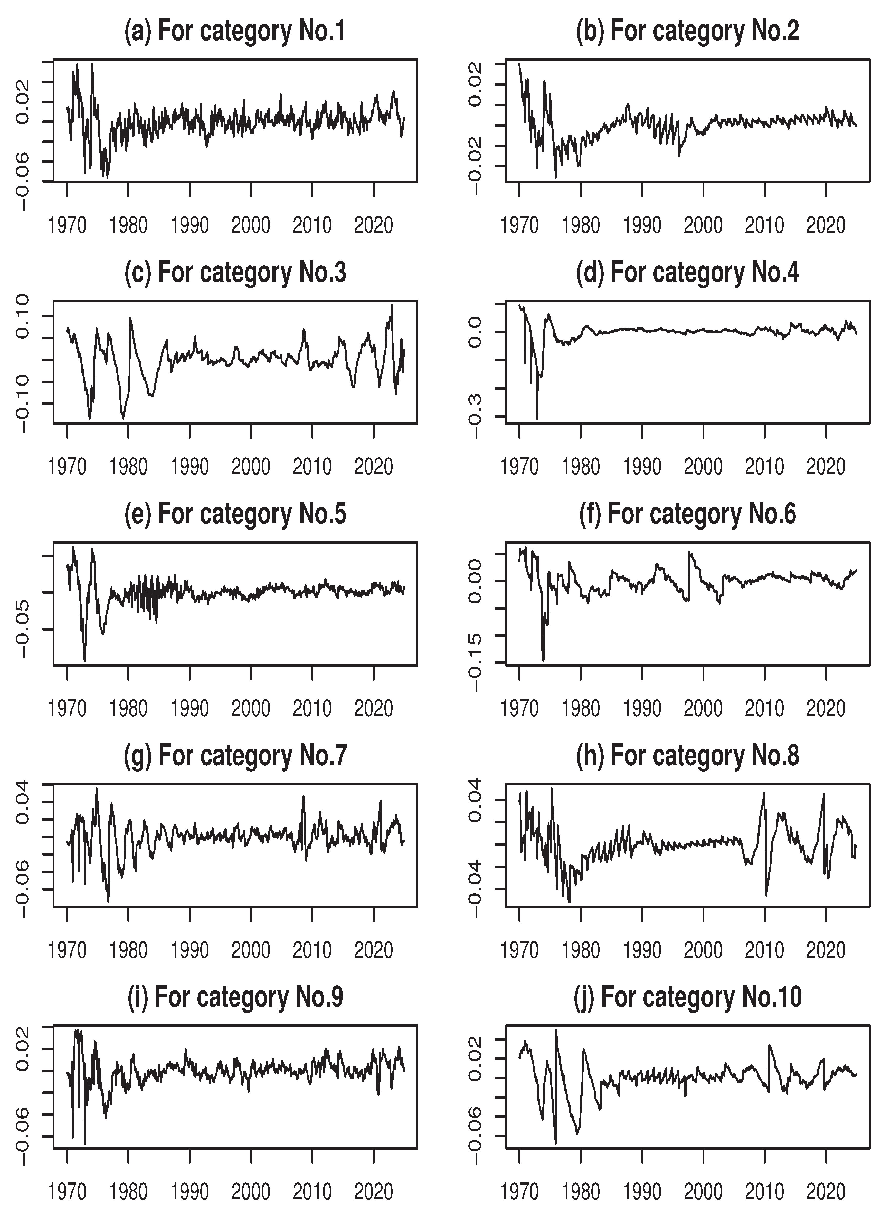
As a reference, the estimated cyclical components for each category are shown in Figure 8 of Appendix D. These results capture the short-term fluctuations in each time series.
To examine the similarities among these cyclical components, we calculated the correlation coefficients between them, as presented in Table 2.
From Table 2, it is evident that the correlations between cyclical components are generally lower than those observed for trend components, indicating that short-term fluctuations are less synchronized across categories. While most category pairs exhibit weak correlations (close to zero), several pairs display moderate positive relationships, exceeding 0.50 – for instance, No. 1 and No. 2 (0.59), No. 3 and No. 10 (0.59), No. 1 and No. 5 (0.51), and No. 2 and No. 5 (0.55). In addition, No. 1 and No. 9 (0.54) also demonstrate a relatively strong association.
4.2.4. Integrated Analysis of Trend, Seasonal, and Cyclical Components
This section provides an integrated comparison of the relationships among Japan’s CPI categories from the perspectives of long-term trends, seasonal fluctuations, and short-term cyclical components. The aim is to highlight how structural, seasonal, and transient factors differentially shape price dynamics across categories.
Firstly, the cluster analysis of trend components indicates that certain category pairs exhibit persistent similarities across multiple periods, reflecting shared structural drivers. For example, the recurring linkage between No. 3 (Fuel, Light, and Water Charges) and No. 10 (Miscellaneous) may be attributed to their common exposure to energy price fluctuations and import cost structures. Similarly, stable associations such as No. 1 (Food) with No. 2 (Housing), and No. 5 (Clothing and Footwear) with No. 9 (Culture and Recreation), point to enduring consumption patterns shaped by household budget allocations, demographic trends, and lifestyle factors. These repeated patterns suggest that trend-level relationships are underpinned by stable socio-economic structures, including energy dependency, long-term shifts in service demand, and durable consumption behavior.
Next, seasonal fluctuations reveal another layer of regularity. In several categories, such as No. 5 (Clothing and Footwear), the amplitude of seasonal variations increased over time, reflecting the strong seasonal demand for products. Across most categories, pattern variability remains high, indicating that seasonal patterns are generally stable, though deviations occur in response to external shocks – e.g., the sharp drop in pattern stability for No. 1 (Food) in 2012, likely due to the lingering effects of the Great East Japan Earthquake or sudden commodity price shifts. Thus, seasonal components capture recurring intra-annual patterns that are largely predictable, yet sensitive to extraordinary events or policy interventions.
Moreover, by contrast, the cyclical components show that short-term correlations among categories are generally weaker, with most pairs exhibiting values close to zero. This suggests the predominance of idiosyncratic or category-specific shocks, such as temporary supply disruptions, commodity price volatility, currency fluctuations, and seasonal demand variations. Nonetheless, a few pairs display moderate positive correlations (above 0.50) – for example, No. 1 (Food) with No. 2 (Housing), No. 3 (Fuel, Light, and Water Charges) with No. 10 (Miscellaneous), and No. 1 (Food) with No. 9 (Culture and Recreation) – indicating that shared short-term drivers, including seasonal events, weather conditions, and energy price shocks, can synchronize temporary movements across specific categories.
Finally, taken together, the integrated analysis reveals a hierarchical structure of price dynamics in Japan’s CPI. Trend components capture long-term structural relationships and enduring socio-economic linkages. Seasonal components reflect predictable intra-year fluctuations, which are largely stable but occasionally disrupted by extraordinary events. Cyclical components, in contrast, respond to temporary, category-specific shocks and exhibit weaker synchronization.
From a policy perspective, this layered understanding suggests that interventions for long-term price stability should target structural relationships among categories, while short-term stabilization policies should focus on mitigating the effects of transient shocks and seasonal extremes affecting specific expenditure groups. The integration of all three components underscores the need for differentiated approaches depending on the time horizon and type of fluctuation being addressed.
To make these contrasts more explicit, a comparative diagram juxtaposing trend-based clusters, seasonal amplitude and pattern variability, and cyclical correlations is included in the conclusion section, visually highlighting the dominance of structural factors in trends, the predictability of seasonal fluctuations, and the sporadic nature of short-term shocks.
5. Concluding Remarks
This study examined the structural dynamics of Japan’s CPI across ten major categories over the period from January 1970 to December 2024. By decomposing each category’s CPI into trend, seasonal, and cyclical components using the integrated ML model approach, we extracted detailed information about long-term structural changes, predictable seasonal patterns, and short-term fluctuations.
Based on the results of the component decomposition and additional analyses, the following key findings were obtained.
- Trend Components: Cluster analysis of trend components revealed persistent similarities among certain category pairs, reflecting stable structural drivers. Notably, No. 3 (Fuel, Light, and Water Charges) and No. 10 (Miscellaneous) exhibited repeated linkages, likely due to shared exposure to energy price movements and import costs. Similarly, pairs such as No. 1 (Food) with No. 2 (Housing) and No. 5 (Clothing and Footwear) with No. 9 (Culture and Recreation) reflected enduring household consumption patterns and lifestyle-driven expenditure behaviors. These results indicate that long-term price dynamics are strongly shaped by underlying socio-economic structures, energy dependencies, and demographic trends.
- Seasonal Components: The seasonal analysis indicated that most categories exhibit stable intra-annual patterns, with generally high amplitude and pattern stability. Exceptions occurred during periods of exceptional external shocks, such as the sharp drop in Food pattern stability in 2012, reflecting disruptions from natural disasters, commodity price shocks, or policy interventions. In categories such as Clothing and Footwear, seasonal amplitudes increased over time, highlighting growing sensitivity to economic maturation and cyclical consumer demand.
- Cyclical Components: In contrast to trend components, cyclical components displayed weaker correlations across categories, indicating that short-term movements are largely idiosyncratic or category-specific. Nonetheless, moderate correlations were observed for a few pairs, such as No. 1 (Food) with No. 2 (Housing) and No. 3 (Fuel, Light, and Water Charges) with No. 10 (Miscellaneous), reflecting shared short-term drivers, including seasonal demand, energy price fluctuations, and temporary supply shocks.
- Integrated Perspective: Taken together, these analyses suggest a hierarchical structure of CPI dynamics: trend components capture long-term structural relationships, seasonal components reflect predictable intra-year cycles with occasional disruption, and cyclical components respond to transient, often category-specific shocks. This integrated view clarifies the relative contributions of structural, seasonal, and transitory factors to overall price dynamics in Japan.
From a policy perspective, these findings suggest that measures aimed at long-term price stability should consider structural linkages among categories, such as energy dependency, demographic trends, and durable consumption behavior. In contrast, mitigating short-term volatility requires targeted interventions addressing transient shocks, seasonal extremes, or sudden commodity price fluctuations affecting specific categories. Moreover, the decomposition framework emphasizes the value of simultaneously analyzing trend, seasonal, and cyclical components to fully understand inflation dynamics and design effective macroeconomic policies.
For future research, this approach can be extended to other countries or regions to enable cross-national comparisons of CPI dynamics. Additionally, incorporating higher-frequency data or alternative disaggregations could provide further insights into intra-sectoral price behavior and the transmission of shocks across categories.
In conclusion, the integrated decomposition of Japan’s CPI over five decades reveals that long-term trends, seasonal patterns, and short-term cycles exhibit distinct yet interrelated behaviors. Recognizing these layered structures enhances both the understanding of inflationary processes and the formulation of effective economic policies. By disentangling structural, seasonal, and transitory influences, this study provides a comprehensive framework for analyzing consumer price dynamics and their socio-economic determinants. Building on these results, a future research goal is to apply the two-lag time-varying loading factor model proposed by Kyo and Noda (2025) to further analyze the mechanisms underlying CPI fluctuations.
Acknowledgments
This work was supported in part by a Grant-in-Aid for Scientific Research (C) (20K01639) from the Japan Society for the Promotion of Science.
Conflicts of Interest
The authors have no relevant financial or non-financial interests to disclose.
Appendix A. Figures for the Used Datasets
Figure A1.
Time series data by category
Appendix B. Figures for the Estimated Trends
Figure A2.
Trends in the time series by category
Appendix C. Figures for the Estimated Seasonal Components
Figure A3.
Seasonal components in the time series by category
Appendix D. Figures for the Estimated Cyclical Components
Figure A4.
Cyclical components in the time series by category
References
- Baxter, M. and King, R. G. (1999), “Measuring Business Cycles: Approximate Band-Pass Filters for Economic Time Series,” Review of Economics and Statistics, 81(4), pp. 575-593.
- Blinder, A. S. (1982), “The Anatomy of Double-Digit Inflation in the 1970s,” In: Hall, R. E. (ed.), Inflation: Causes and Effects, University of Chicago Press, pp. 261-287.
- Boskin, M. J., Dulberger, E. L., Gordon, R. J., Griliches, Z., and Jorgenson, D. W. (1998), “Consumer Prices, the Consumer Price Index, and the Cost of Living,” Journal of Economic Perspectives, 12(1), pp. 3-26.
- Bryan, M. F. and Cecchetti, S. G. (1993), “The Consumer Price Index as a Measure of Inflation,” NBER Working Paper, No. 4505.
- Hale, G. B. and Jorda, O. (2007), “Do Monetary Aggregates Help Forecast Inflation? FRBSF Economic Letter, No. 2007-10, pp. 1-3.
- Harvey, A. C. (1990), Forecasting, Structural Time Series Models and the Kalman Filter, Cambridge University Press.
- Ito, T. and Hoshi, T. (2020), The Japanese Economy, 2nd Edition, The MIT Press.
- Kyo, K. (2025), “Reinforcing Moving Linear Model Approach: Theoretical Assessment of Parameter Estimation and Outlier Detection,” Axioms, 14(7), 479. [CrossRef]
- Kyo, K. and Kitagawa, G. (2023), “A Moving Linear Model Approach for Extracting Cyclical Variation from Time Series Data,” Journal of Business Cycle Research, 19(3), pp. 373-397.
- Kyo, K. and Noda, H. (2025), “Analyzing Mechanisms of Business Fluctuations involving Time-Varying Structure in Japan: Methodological Proposition and Empirical Study,” Computational Economics. [CrossRef]
- Kyo, K., Noda, H., and Fang, F. (2024), “An Integrated Approach for Decomposing Time Series Data into Trend, Cycle and Seasonal Components,” Mathematical and Computer Modelling of Dynamical Systems, 30(1), pp. 792-813.
- Stock, J. H. and Watson, M. W. (2016), “Dynamic Factor Models, Factor-Augmented Vector Autoregressions, and Structural Vector Autoregressions in Macroeconomics,” In: Taylor, J. and Uhligpp, H. (eds.), Handbook of Macroeconomics, vol. 2, Elsevier, pp. 415-525.
| 1 | Boskin et al. (1998) state at the beginning of their article as follows: Accurately measuring prices and their rate of change, inflation, is central to almost every economic issue. There is virtually no other issue that is so endemic to every field of economics. |
| 2 | In Japan, several large financial institutions failed in 1997–1998, causing severe financial turmoil, with a heightened premium that Japanese banks had to pay in interbank transactions, and the damaged financial system put the Japanese economy into a deflation starting in 1998 (see Ito and Hoshi, 2020, Ch.6). |
| 3 | Because, from the mid-1970s to the mid-1980s, Japan experienced very stable economic growth though at lower levels than the rapid economic growth period, Ito and Hoshi (2020) refer to this period as “the moderate growth period” or “great moderation in Japan.” |
Figure 1.
Time series of differenced estimated trends by category
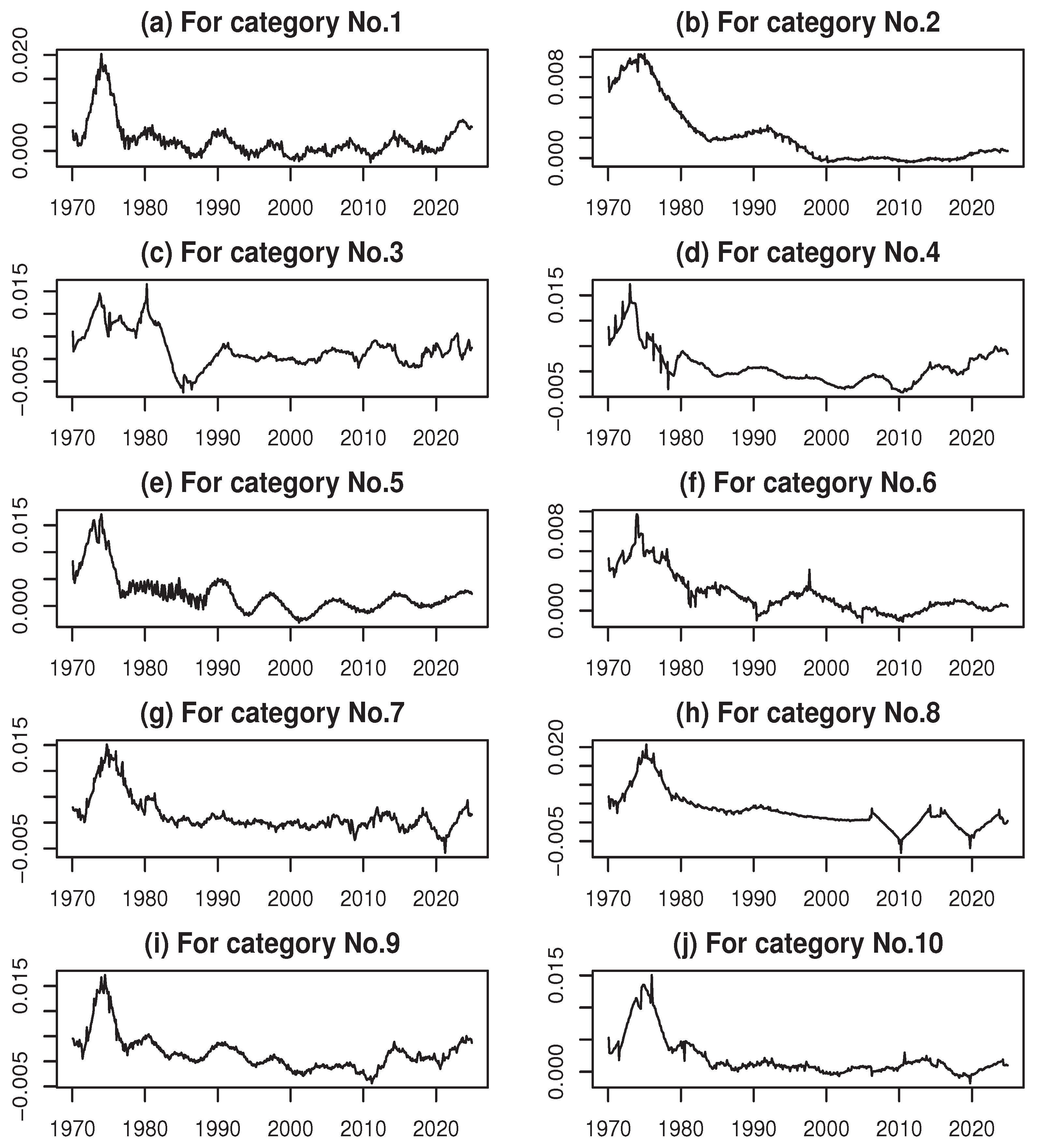
Figure 2.
Cluster analysis of ten category’s CPI by period
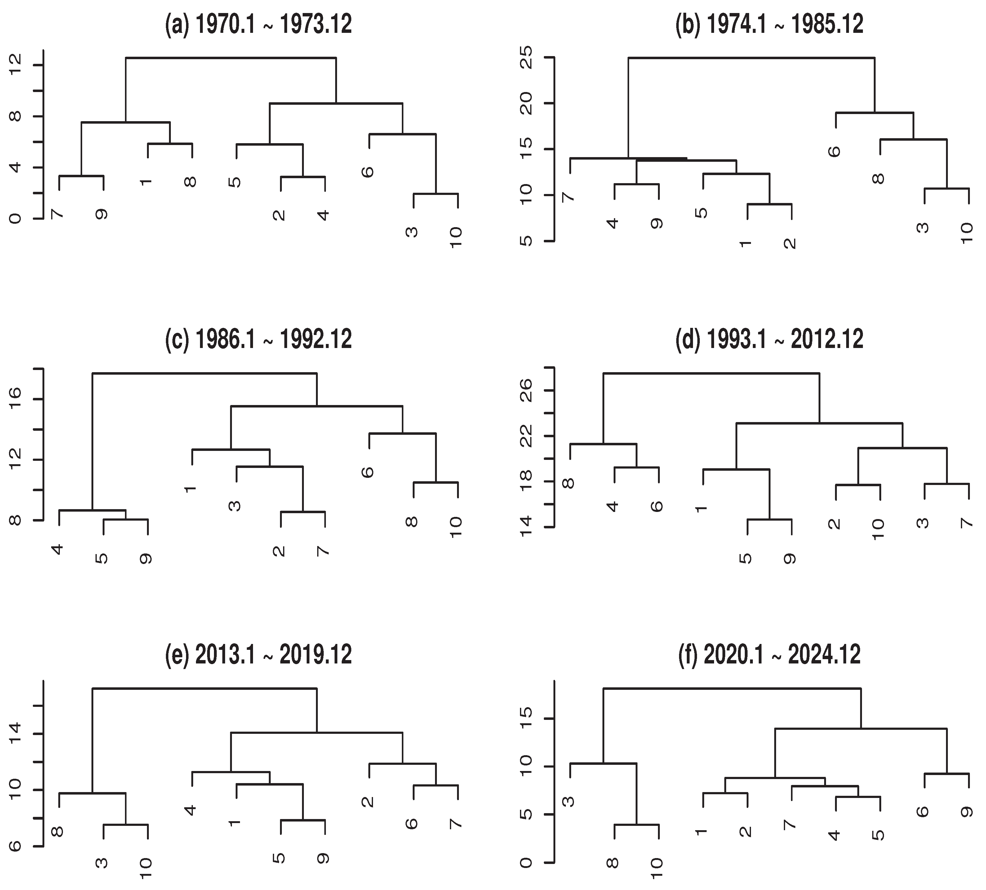
Figure 3.
Time series of amplitude variabilities in the seasonal components
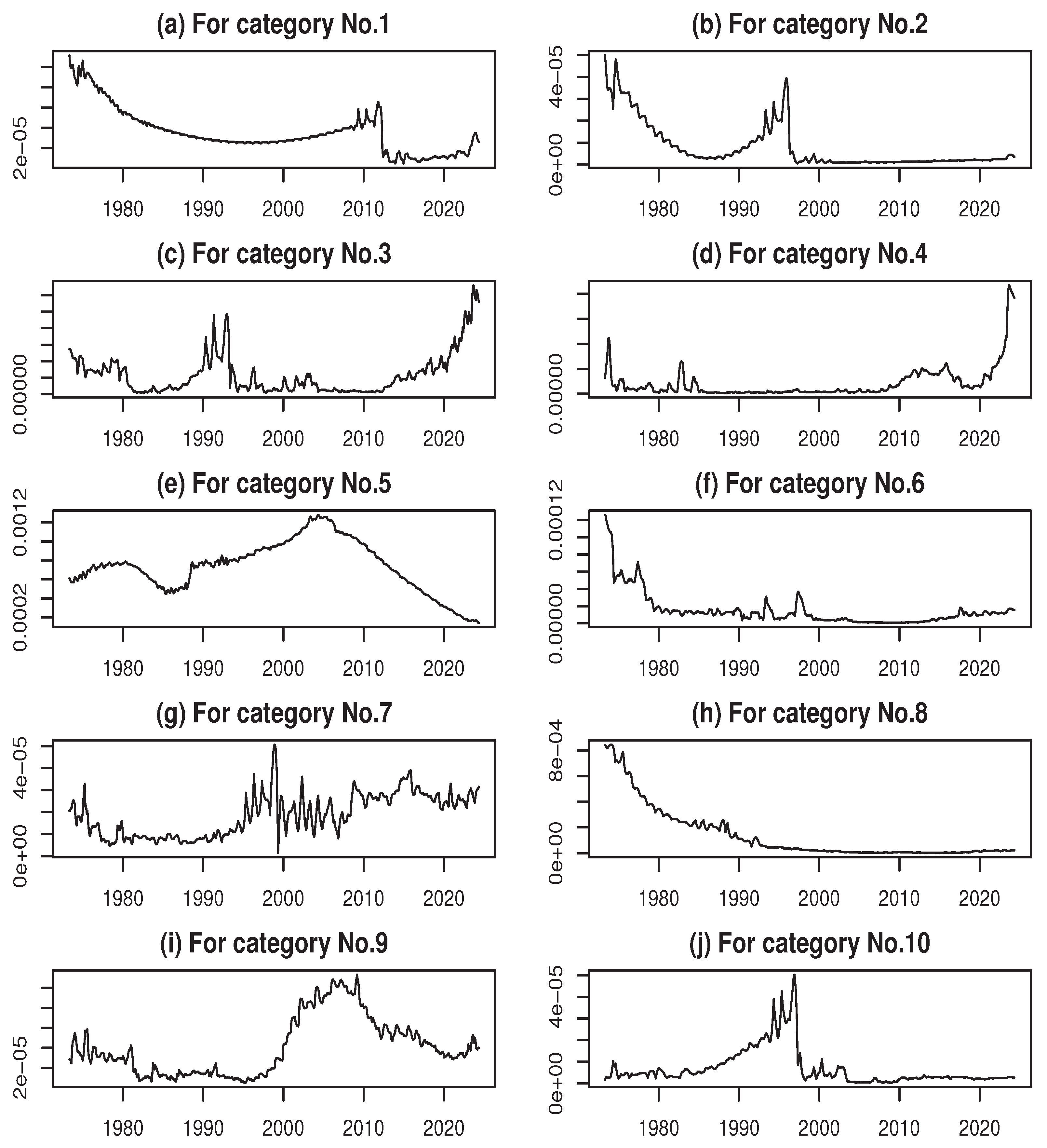
Figure 4.
Time series of pattern variabilities in the seasonal components
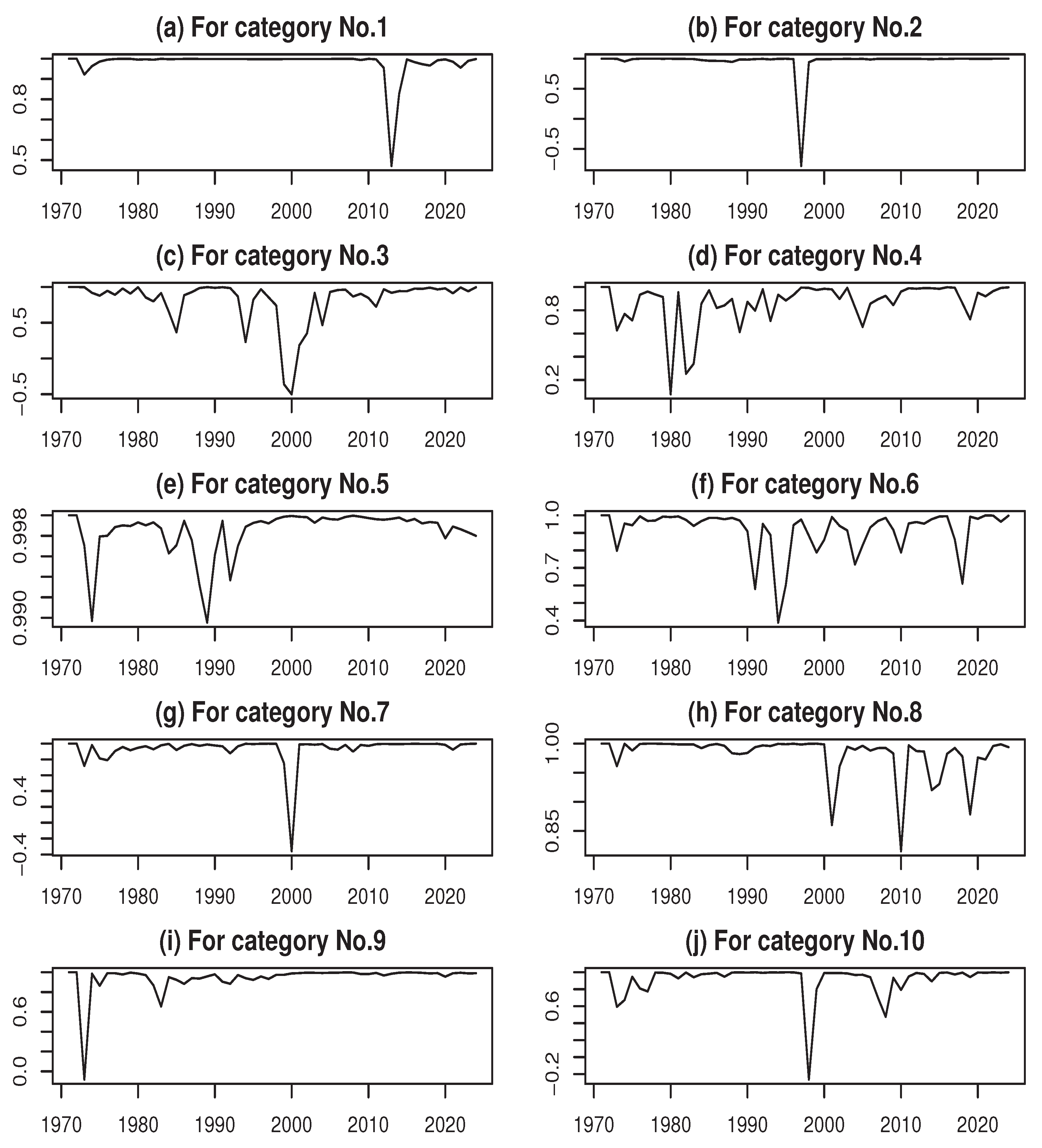

Table 1.
Major categories of the CPI in Japan
| No. | Category |
|---|---|
| 1 | Food |
| 2 | Housing |
| 3 | Fuel, Light, and Water Charges |
| 4 | Furniture and Household Utensils |
| 5 | Clothing and Footwear |
| 6 | Medical Care |
| 7 | Transportation and Communication |
| 8 | Education |
| 9 | Culture and Recreation |
| 10 | Miscellaneous |
Table 2.
Correlation coefficients between estimated cyclical components
| No.1 | No.2 | No.3 | No.4 | No.5 | No.6 | No.7 | No.8 | No.9 | No.10 | |
|---|---|---|---|---|---|---|---|---|---|---|
| No.1 | 1.00 | 0.59 | 0.18 | 0.36 | 0.51 | 0.06 | 0.45 | 0.23 | 0.54 | 0.36 |
| No.2 | 1.00 | 0.32 | 0.52 | 0.55 | 0.20 | 0.34 | 0.39 | 0.43 | 0.49 | |
| No.3 | 1.00 | 0.40 | 0.13 | 0.21 | 0.20 | 0.29 | 0.17 | 0.59 | ||
| No.4 | 1.00 | 0.48 | 0.12 | 0.26 | 0.15 | 0.36 | 0.36 | |||
| No.5 | 1.00 | -0.10 | 0.26 | 0.13 | 0.33 | 0.29 | ||||
| No.6 | 1.00 | 0.06 | 0.20 | 0.13 | 0.23 | |||||
| No.7 | 1.00 | 0.11 | 0.40 | 0.19 | ||||||
| No.8 | 1.00 | 0.29 | 0.31 | |||||||
| No.9 | 1.00 | 0.24 |
Disclaimer/Publisher’s Note: The statements, opinions and data contained in all publications are solely those of the individual author(s) and contributor(s) and not of MDPI and/or the editor(s). MDPI and/or the editor(s) disclaim responsibility for any injury to people or property resulting from any ideas, methods, instructions or products referred to in the content. |
© 2025 by the authors. Licensee MDPI, Basel, Switzerland. This article is an open access article distributed under the terms and conditions of the Creative Commons Attribution (CC BY) license (http://creativecommons.org/licenses/by/4.0/).
Copyright: This open access article is published under a Creative Commons CC BY 4.0 license, which permit the free download, distribution, and reuse, provided that the author and preprint are cited in any reuse.


