
Submitted:
23 July 2025
Posted:
24 July 2025
You are already at the latest version
Abstract
Debris flow events are complex natural phenomena that are challenging to predict, especially when data are limited or uncertain. This study presents a novel Bayesian probabilistic approach using Bayesian Neural Networks (BNNs) to predict possible volumes of debris flow accumulation by integrating both synthetic and real-world data. Synthetic datasets are created based on statistical distributions informed by geomorphological and hydrological knowledge, allowing the model to learn typical behaviors even with limited real data. BNNs provide uncertainty quantification by modeling neural weights as probability distributions. The models resulting from validation on synthetic data and two real datasets from China and South Korea show strong predictive performance (R² > 0.99) and close alignment between predicted and observed volumes, even in the presence of outliers. Our framework for generating synthetic data allows for the creation of context-specific datasets, calibrating the statistical parameters of debris flows for each territory. These specific datasets allow for the creation of specific predictive models; however, some models can be transferred between regions similar in geological, climatic and geomorphological characteristics, even with the absence or scarcity of data. The key strength of this integrated approach lies in its integration of synthetic data generation, real data augmentation based on Bootstrapping, expert knowledge and Bayesian deep learning to overcome limitations of traditional statistical models, improving debris flow forecasting and enabling more informed and resilient risk management strategies.
Keywords:
debris flow
; Bayesian neural networks (BNN)
; synthetic data generation
; uncertainty quantification
; probabilistic modeling
; risk assessment
; deep learning in geosciences
1. Introduction
This paper is framed of the LanDam project financed with PNRR funds in the RETURN Extended Partnership - Multi-Risk sciEnce for resilienT commUnities undeR a changiNg climate- Spoke 2. In particular, methodological issues related to potentially occluding landslide phenomena of riverbeds with their upstream and downstream impacts of damming are investigated. The research starts from the primary consideration of debris-flow type landslide phenomena, which represent types of landslides that are difficult to interpret both in the prediction and paroxysmal evolution phases. This work aimed to propose a probabilistic approach for the prediction of accumulation volumes using a Bayesian Neural Networks with Synthetic and Real-World Data Integration.
In recent years, Artificial Intelligence (AI) has increasingly been applied in geosciences to model complex natural phenomena, thanks to its ability to process large datasets and uncover both linear and nonlinear relationships among variables [1]. Among AI techniques, Artificial Neural Networks (ANNs) have gained particular attention due to their biological inspiration and strong performance in pattern recognition and predictive tasks. Their use has been proven effective in hydrology [2], sediment transport [3], debris flow susceptibility [4], and flood prediction [5]. However, the application of AI to debris flow prediction remains limited, primarily due to the intrinsic complexity of these events characterized by high spatial and temporal variability, nonlinearity, and uncertainty in triggering conditions [6].
A debris flow is a type of mass wasting process that acts on natural and engineered slopes. It is the movement of a mass of rock, dry or wet debris, under the influence of gravity [7]. Debris flows involve flowing, sliding, toppling, falling, or spreading, and many debris flows exhibit a combination of different types of movements, at the same time or during the lifetime of the debris flow. Debris flows are present in all continents and play an important role in the evolution of landscapes. In many areas they also pose a serious threat to the population. Predicting the magnitude and accumulation volume of such events is essential for risk assessment and civil protection planning but is hindered by data scarcity, especially in regions where events are infrequent or monitoring infrastructures are lacking [8]. In addition, any accumulation of material along riverbeds affected by neighboring, earth flow, wet or dry debris flow, could obstruct the path of the river causing its overflow. Traditional numerical, empirical or physically based models often struggle to generalize across different geographic contexts due to their deterministic nature and rigid parameterizations [9].
Mathematical and numerical modeling is extensively employed to study debris flows, enabling analysis of their evolution, forecasting, and impact assessment. These models are grounded in differential equations derived from conservation laws (mass, momentum, and energy), often supplemented by empirical or theoretical closure relations. Among the most advanced approaches is the Unsteady Reynolds-Averaged Navier-Stokes (URANS) model within Computational Fluid Dynamics (CFD) [10], also used for simulating sediment transport in both laminar and turbulent regimes [11]. However, due to the computational time demands of full 3D models, simplified frameworks like the Shallow Water equations [12] or Reduced Complexity Models (RCMs), such as Cellular Automata (CA) [13], are frequently adopted.
Discretization of the system domain, typically via mesh-based methods using simple geometric elements, is essential for calculating physical quantities such as stress, velocity, and flow height. Common discretization techniques include the Finite Element Method (FEM) [14], Finite Difference Method (FDM), Finite Volume Method (FVM), and Boundary Element Method (BEM). Mesh-free approaches, like Smoothed Particle Hydrodynamics (SPH) [15,16,17,18], and hybrid techniques such as the Particle Finite Element Method (PFEM) [19,20,21], offer alternatives that bypass the complexities of mesh generation.
For modeling mudflows involving sediment and granular transport, Computational Granular Dynamics is particularly effective, treating materials as interacting particles ranging, in size, essentially, from microns to centimeters. Given the inherent variability and uncertainty in physical and geo-mechanical parameters, probabilistic approaches, especially the Monte Carlo Method [22,23,24], are widely used for stochastic simulations. Additionally, statistical tools support the analysis of sediment grain size distributions in debris flows [25].
To address these challenges, we propose to apply a novel probabilistic approach based on Bayesian Neural Networks (BNNs). In the Bayesian framework, probability represents a degree of belief or confidence in the occurrence of an event. As new evidence is obtained, this belief is updated through Bayes' theorem, which serves as the fundamental principle for refining, updating and improving these probability estimates [26]. BNNs extend traditional ANNs by incorporating uncertainty directly into model parameters, treating network weights as probability distributions rather than fixed values [27]. This feature allows not only accurate predictions, but also for an explicit quantification of the model’s confidence in its outputs (an essential capability in risk-sensitive decision-making, [28]).
Furthermore, to overcome the limitations imposed by small datasets, we integrate the use of synthetic data generation, leveraging both bootstrapping methods [29] and domain-based assumptions to create plausible input scenarios. These synthetic datasets are designed to preserve the statistical and physical properties of real-world variables influencing debris flow dynamics (e.g., slope, rainfall intensity, soil type, lithology), allowing the model to learn typical behavior patterns even when empirical data is insufficient.
This study proposes a two-step framework: (1) the generation and validation of synthetic datasets using statistical distributions informed by geomorphological and hydrological knowledge; (2) the implementation and training of a Bayesian Neural Network to predict debris flow accumulation volumes, first tested on the synthetic dataset and subsequently validated on two real-world datasets from China [30] and South Korea [31].
The proposed framework demonstrates an innovative approach to debris flow prediction that combines strong generalization capabilities with robust uncertainty quantification and demonstrates promising performance across diverse geomorphological contexts. A key element of our methodology is the use of synthetic data generation (especially where real data is scarce), which enables the creation of tailored datasets for specific geographical areas by calibrating parameters that statistically describe the debris flow phenomenon. This allows for the development of local predictive models even in the absence of real observations. By integrating these synthetic datasets within a Bayesian framework, we obtain highly specific probabilistic predictions of volume accumulation. This adaptability represents a core strength of our approach, offering a flexible and scalable solution for hazard assessment. While regions with similar characteristics may benefit from shared models, the most accurate and context-aware predictions are achieved through the generation of region-specific synthetic data and corresponding dedicated models.
2. Materials and Methods
This section details the methodology adopted for synthetic data generation and the application of advanced deep learning models, specifically Bayesian Neural Networks (BNNs), for debris flow volume prediction.
The primary objective was to develop a robust framework for debris flow modeling that not only provides accurate predictions but also quantifies the associated uncertainty, a crucial aspect in geoscientific applications where the intrinsic variability of natural phenomena is significant. The methodology is organized into several key phases, briefly outlined below and discussed in greater detail in the subsequent sections.
Synthetic Data Generation (Section 2.1): This describes the creation of an artificial dataset that replicates the statistical properties and inter-variable relationships of real debris flow data, enabling rigorous model evaluation in a controlled setting
Bayesian Neural Network Modeling (Section 2.2): This delves into the theory and implementation of Bayesian Neural Networks, emphasizing their capability to quantify predictive uncertainty, a distinct advantage over traditional neural networks.
Application of Bayesian Neural Networks (Section 2.3): This section presents the unified application of BNNs to synthetic and real debris flow data, detailing data preparation, model design, training, and uncertainty quantification, with a focus on reproducibility and methodological transparency.
2.1. Synthetic Data Generation
This section outlines the methodology for generating a synthetic dataset meticulously designed to replicate key statistical characteristics observed in debris flow related parameters. The primary aim was to establish a controlled and reproducible environment for the subsequent evaluation of predictive models, ensuring the synthetic data accurately reflected realistic inter-variable dependencies and probabilistic distributions inherent in natural phenomena.
2.1.1. Modeling of Independent Variables and Distributions
Eight independent variables, crucial for debris flow and debris-flow susceptibility and dynamics, were synthesized. Each variable's distribution was carefully chosen and parameterized to mimic observed geophysical properties, referencing established literature.
Rainfall: extreme rainfall events, recognized as primary triggers for debris flows, were modeled using a truncated power-law distribution. This distribution is particularly effective due to its ability to capture the heavy-tail behavior characteristic of high-magnitude, low-frequency precipitation events, consistent with observations across various climatic regions [32]. For this model, proper coefficients were utilized, ensuring a realistic decay for high intensity events. The rainfall values, representing 24-hour accumulations, were bounded between 50 mm and 600 mm , reflecting physically plausible rainfall intensities capable of triggering debris flows.
Grain Size: The diameter of sediment grains is represented by a log-transformed and truncated Generalized Hyperbolic (GH) distribution. The GH distribution is a flexible family of continuous distributions that can be defined using the following probability density function (pdf) [33], reported as an example of the kind of distribution we have used:
Where: is the logarithmic value of the sediment grain diameter; shape index; scale parameter; asymmetry parameter; position and scale position; modified Bessel function of the second kind of zero order. Then the expression was normalized. Figure 1 shows the related plot.
This approach aligns with common models for particle-size distributions in natural sediments, such as those found in debris flows [33]. This specific distribution is chosen because it effectively captures both the asymmetry and heavy tails frequently observed in granulometric datasets. To reflect real-world material size ranges, the distribution is truncated with limits set between 0.1 mm and 100 mm. This detailed representation of particle diameter is crucial as it directly influences material strength and permeability.
Soil Composition: This variable, representing overall composition of fine content, was simulated using a Beta distribution scaled between 0% and 100%. This broad range allows for the representation of diverse soil types, from cohesionless to cohesive, as supported by studies on soil parameter variability [34].
Friction Angle (ϕ): This is a crucial parameter in debris flow analysis, is modeled using a truncated normal distribution [9]. This approach ensures that the generated values remain within geotechnically valid bounds while preserving natural variability, reflecting observations on real phenomena. Specifically, the distribution is centered around 30° with a standard deviation of 5°. The values are restricted to a physically meaningful and realistic interval between 20° and 45°, corresponding to typical friction angles found in natural soils. This constraint is vital for maintaining the physical realism of the model.
Friction (μ): a critical parameter for granular flow, is modeled using a scaled Beta distribution [12]. This choice is particularly appropriate for variables naturally bounded between two values, allowing for accurate representation of its skewed nature and defined domain. The assumed distribution is characterized by a right-skewed shape. This skewness implies that lower friction values are more probable, which is reflective of conditions often found in saturated or loose soils. The generated values are then rescaled to the interval [0.05, 0.4], which corresponds to typical friction coefficients observed in both granular and cohesive soils.
Slope Angle (θ): a primary control parameter on debris flow initiation and evolution, is modeled using a truncated normal distribution. This approach aligns with observed distributions in various morphological contexts, ensuring that generated slopes are both plausible and diverse [35]. Specifically, the slope angle is drawn from a distribution centered at 25° with a standard deviation of 7°. The values are constrained to a physically realistic range, truncated between 10° and 45°. These limits reflect the natural range of hillslope gradients typically associated with debris flows.
Density (): a key factor in estimating mass movement dynamics, is simulated using a truncated normal distribution. This approach incorporates typical values observed for various geotechnical materials, from loose mud to denser rocky debris. Specifically, the distribution has a mean of 1800 kg/m³ and a standard deviation of 150 kg/m³. The values are bounded between 1300 kg/m³ and 2300 kg/m³ to reflect the realistic range of densities found in granular and cohesive soils [12].
Visco-Turbulent Parameter (ξ) (adimensional): The visco-turbulent parameter (ξ), which distinguishes between wet and dry debris flows, is generated by sampling from a mixture of triangular distributions. This approach effectively captures the bimodal behavior observed in landslide dynamics [12]. The simulation randomly selects between "granular" and "earth flow" regimes with equal probability (=0.5). For granular flows ξ values range from 100 to 200, with a peak at 150. Conversely, for earth flows, ξ ranges from 200 to 1000, peaking at 500. This method ensures that the generated values reflect the flow-type-dependent resistance, encompassing both viscous and turbulent effects.
A comprehensive overview of the synthetic data generation framework, obtained through Python language, is provided in Figure 2.
2.1.2. Imposition of Inter-Variable Correlation Structure
To assign realistic interdependencies among the variables in our synthetic dataset, we predefined a Pearson cross-correlation matrix based on assumed variable relationships. To ensure mathematical validity for the subsequent steps, this matrix underwent a positive-definite adjustment using the "nearest positive definite" algorithm [36]. The process involved generating a set of initially uncorrelated variables. These were then transformed to achieve the desired correlations using the Cholesky decomposition [37] of the adjusted matrix. Cholesky decomposition breaks a symmetric, positive-definite matrix (no negative eigenvalue) into a lower triangular matrix and its transpose for efficient computation. If the matrix is not positive-definite, a nearest positive definite adjustment (NPDA) modifies it to the closest valid matrix to enable decomposition. NPDA is a technique used to modify a symmetric matrix (like a covariance matrix) so that it becomes positive definite, meaning all its eigenvalues are positive (in terms of Frobenius Norm). For distribution imposition, the correlated variables were first converted to uniformly distributed variables via the cumulative distribution function (CDF). Finally, we applied the inverse CDF for each target distribution, ensuring that the synthetic data matched both the specified distributions and the intended correlation structure
2.1.3. Dependent Variable Volume Generation
The Volume of the debris flow accumulation was assumed as the dependent variable, generated as the predicted output of a specialized neural network model, rather than derived from a direct, explicit experimental, numerical or analytical formula. We adopted this approach to simulate volumes exhibiting non-linear characteristics consistent with real-world debris-flow phenomena, specifically their observed heavy-tailed (power-law) distributions behavior [38].
The total volume available for the debris flow is implicitly accounted for within the variability range used in the simulations. This range reflects both the mass generated by instability and the balance between erosion and deposition. Different numerical values can be used to represent other scales. The input is directly provided by the user, who is expected to have geological, engineering, or related knowledge of the system.
The neural network's architecture included a custom layer with specific weight constraints, followed by standard dense layers with ReLU (Rectified Linear Unit) activation function and a final output layer with softplus activation to ensure positive volume predictions. The network was constrained to maintain correlations by attempting to predict the power-law distribution, minimizing the Kullback-Leibler (KL) [39] between the predicted volume distribution and a target power-law distribution. This implicitly calibrated the relationship between the independent variables and the resulting synthetic volumes.
2.2. Bayesian Neural Network Architecture
In this section, we outline the fundamental aspects of the Bayesian Neural Network (BNN) architecture, focusing on both the underlying theory and its implementation in Python.
2.2.1. “Bayes by Backprop”: Weight Uncertainty in Neural Networks [40].
Traditional ANN, unlike their Bayesian counterparts, provides point estimates for their weights and biases. This means that each weight or bias parameter is represented by a single, deterministic value, leading to single-point predictions without an inherent measure of uncertainty. This limitation is particularly critical in safety-sensitive applications like natural hazard prediction, where understanding confidence in a prediction is as important as the prediction itself. The BNN meets this need by placing probability distributions over the network’s weights and biases, enabling the quantification of predictive uncertainty (Figure 3).
In a BNN, instead of learning fixed weight values, the primary goal is to infer the posterior distribution over the weights, , given the observed data, where represents the network weights and is the dataset. Directly computing this true posterior is analytically intractable due to the high dimensionality of the weight space and the non-linearity of neural networks. Consequently, Variational Inference (VI) is commonly employed to approximate the true posterior with a simpler, tractable distribution, parameterized by [40]. Here, is referred to as the variational distribution or approximate posterior distribution. The objective of VI is to minimize the KL divergence between the approximate posterior and the true posterior :
The KL divergence, KL], measures the “distance” or information gain between the two distributions. The resulting cost function is variously known as the variational free energy [41,42,43] or the expected lower bound [44,45]. For simplicity (eq. 1) could be denoted as:
Where KL is the complexity cost which acts as a regulator, encouraging the approximate posterior to remain close to the chosen prior distribution over the weights, ), helping to prevent overfitting and promoting more robust models [40]. The complexity cost reflects the "complexity" of the model in terms of how much it deviates from our prior knowledge about the weights; is the likelihood cost, often referred to as the expected negative log-likelihood, encourages the model to fit the training data well, representing how well the model, with its sampled weights, explains the observed data. The total cost function (eq. 3) embodies a trade-off between satisfying the complexity of the data (by minimizing the likelihood cost) and satisfying the simplicity prior (by minimizing the complexity cost). Exactly minimizing this cost naively is computationally prohibitive. Instead, gradient descent and various approximations are used [40]. During training, samples of weights are drawn from the approximate posterior distribution . Gradients are then backpropagated through the network to update the variational parameters of this approximate posterior. This specific training procedure, where the variational parameters are updated via backpropagation, is known as "Bayes by Backprop" [40]. This method allows for efficient training of BNNs by leveraging standard gradient-based optimization techniques.
Once the BNN is trained, predictive uncertainty can be estimated by performing multiple forward passes (stochastic inferences) through the network. This process, often referred to as Monte Carlo Sampling from the Approximate Posterior distribution [40], provides a robust measure of the model's uncertainty. For a given input, multiple sets of outputs are sampled from the learned approximate posterior, leading to an ensemble of predictions. The mean of these predictions provides the most probable output, while the standard deviation quantifies the predictive uncertainty [40].
2.2.2. Implementation of "Bayes by Backprop" in TensorFlow
Implementing "Bayes by Backprop" in TensorFlow (and Keras) is significantly facilitated by libraries like TensorFlow Probability (TFP). TFP provides the necessary building blocks for constructing probabilistic models, including neural network layers with distributed weights. Here the key steps are briefly outlined below for conceptual implementation
Defining Bayesian Layers: Instead of traditional Keras layers like Dense or Conv2D which have deterministic weights, one uses TFP's specialized layers such as tfp.layers.DenseVariational. These layers do not learn a single weight value but rather the parameters of a distribution (e.g., mean and standard deviation for a Gaussian distribution) from which the weights will be sampled during inference and training [40].
Defining the Approximate Posterior Distribution: For each weight in the network, we must define how its posterior distribution will be approximated. TensorFlow Probability makes this straightforward by allowing “kernel_posterior_fn” and “bias_posterior_fn” to be specified within the variational layers. These functions define the distribution from which weights will be sampled and how its parameters will be learned. [40].
Defining the Prior Distribution (): Similarly, “kernel_prior_fn” and “bias_prior_fn” define the prior distribution for the weights and biases. [40].
Sampling and Propagation: During the model's forward pass, the variational layers sample weights from their approximate posterior distributions. These sampled weights are then used for computations just as in standard ANN. This sampling process introduces the necessary stochasticity to estimate uncertainty.
Defining the Loss Function: The loss function is the sum of the likelihood cost and the complexity cost. TensorFlow Probability automatically handles the calculation of the KL term (the complexity cost) when using its variational layers. The likelihood cost is typically the negative log-likelihood of the model on the data (e.g., tfp.losses.NegativeLogLikelihood for distributions). These two terms are combined to form the cost function [40].
Optimization: A standard optimizer (such as Adam or SGD) is used to minimize the loss function. Gradients are computed with respect to the variational parameters (θ, i.e., the means and standard deviations of the weight distributions) and update these parameters to bring closer to [40].
Predictive Uncertainty: After training, to obtain uncertainty estimates, a code with multiple forward passes is executed on the same input. Each pass will sample a new set of weights from the learned distribution, leading to slightly different predictions. The mean of these predictions provides the point estimate, while the variance or standard deviation of the predictions provides the measure of uncertainty [40]. In practice, TensorFlow Probability greatly simplifies this process, abstracting away much of the complexity of sampling and KL divergence calculation, allowing scientists, engineers and developers to focus on defining the model and its architecture.
An overview of Section 2.2 is illustrated in the light blue flowchart on the left side of Figure 4.
2.3. Application of Bayesian Neural Networks
This section describes the application of Bayesian Neural Networks (BNNs) for predicting debris flow volumes using both the synthetically generated dataset and real-world debris flow datasets (Flow-chart reported in Figure 4). The entire prediction framework was developed in Python, primarily utilizing the TensorFlow and TensorFlow Probability libraries, ensuring a consistent approach across different data types.
2.3.1. Data Preparation and Preprocessing
For both synthetic and real-world datasets, a meticulous preprocessing pipeline was applied. All independent variables were scaled using z-score normalization (standardization). The dependent variable, debris flow volume, exhibiting a heavy-tailed distribution, was first subjected to a logarithmic transformation to reduce skewness and stabilize variance, and subsequently also scaled with z-score normalization. These preprocessing steps are crucial for ensuring numerical stability during training, improving convergence speed, and for conforming the target distribution more closely to the assumptions of neural networks. The pre-processed data was then split into training (calibration) (80%) and testing sets (validation) (20%) to evaluate generalization performance.
2.3.2. Bayesian Neural Network Architecture
A consistent Bayesian Neural Network model was constructed using Dense Variational layers, which inherently introduce a probability distribution over the network's weights and biases. The model architecture comprised multiple hidden Dense Variational layers with appropriate activation functions. Specifically, for the Prior Distribution “kernel_prior_fn” and “bias_prior_fn” were defined. For the Approximate Posterior Distribution ”kernel_posterior_fn” and “bias_posterior_fn” were defined. The “kl weight” for each Dense Variational layer was set in relation to the number of samples in the training set (by scaling with the number of training samples), following best practices to balance the likelihood and KL divergence terms in the cost function. The model used a final Dense output layer with a single unit to predict the mean of the transformed volume. Compiled with the Adam optimizer and the cost function loss, the model also incorporated the Huber loss function. Huber loss was selected for its superior robustness to outliers, a valuable characteristic when handling potentially noisy or heavy-tailed target variables.
2.3.3. Training, Evaluation, and Uncertainty Analysis
The training protocol involved an initial hyperparameter search over a limited grid (e.g., varying learning rates, activation functions, and number of layers). The model yielding the lowest validation loss was selected as the "best model" based on its performance on unseen validation data. Subsequently, this best model was retrained on the full training dataset for an extended number of epochs (in AI, epochs refer to the number of complete passes through the entire training dataset during the learning process of a model) to ensure thorough convergence and optimize its parameters.
Predictive uncertainty was quantified by performing multiple stochastic forward passes through the trained model. For each test sample, 100 forward passes were executed. During each pass, weights were sampled from their learned posterior distributions. The mean and standard deviation of these predictions were then calculated for each test sample, providing both the most probable prediction and a measure of its uncertainty. The predicted mean and standard deviation values were then inverse-transformed back to the original volume scale, taking into account the prior logarithmic and z-score transformations. This allows for direct interpretation of predictions and uncertainty in their original units (e.g., cubic meters).
The performance of the BNN model was evaluated using several established metrics and comprehensive visualizations. These included the calculation of Mean Squared Error Percentage (MSE%) and Coefficient of Determination () to assess prediction accuracy.
The Mean Squared Error Percentage (MSE%) is a variation of the Mean Squared Error (MSE) that expresses the error as a percentage, often to make it more interpretable and comparable across different scales of data. The following is the common formula for MSE% (eq. 4):
Where is the number of observations, is the actual (observed) value for the i-th observation and is the predicted value for the i-th observation.
The formula (eq. 5) for the coefficient of determination,, is a fundamental concept in linear regression, both simple and multiple. It indicates the proportion of the variance in the dependent variable that can be explained by the regression model. Several equivalent formulas exist for calculating but the most common and intuitive is the following:
Where (eq. 6) (Sum of Squared Residuals) represents the variation not explained by the model. It is the sum of the squares of the differences between the observed values of the dependent variable () and the values predicted by the model :
And (eq. 7) (Total Sum of Squares) represents the total variation in the dependent variable. It is the sum of the squares of the differences between the observed values of the dependent variable () and the mean of the dependent variable ():
is a value between 0 and 1 (or 0% and 100%). An close to 1 indicates that the regression model explains a large percentage of the variability in the dependent variable. In other words, the model fits the data well. An close to 0 indicates that the regression model explains a small or no percentage of the variability in the dependent variable. The model is not very useful for predicting the dependent variable.
Visualizations included generation of observed vs predicted plots to visually inspect agreement and histograms with Kernel Density Estimation (is a non-parametric method to estimate the probability density function of a random variable based on a finite data sample.) of the predictions. All results, trained model parameters, and learned weight distributions were saved for full reproducibility and detailed post-analysis.
2.3.4. Application to Synthetic Data
The framework described above was first applied to the synthetic dataset generated in Section 2.1. This allowed for a controlled environment to rigorously evaluate the predictive capabilities and uncertainty quantification of the BNN model under ideal conditions, where the true underlying data characteristics were known. For training purposes, 10,000 samples were synthetically generated, with 8,000 for training (calibration) and 2,000 for testing (validation).
2.3.5. Application to Real-World Debris Flow Data
Subsequently, the BNN framework was applied to real-world debris flow datasets from the Sichuan region in China and from South Korea.
The dataset sourced from [30] comprises observed debris flow events in the Sichuan region of China, specifically focusing on 60 typical debris-flow catchments that experienced events between 2008 and 2018. This dataset is characterized by variables such as basin area (A), topographic relief (H), channel length (L), distance from nearest seismic fault (D), and average channel slope (J). These morphological factors were measured using ArcGIS from 10-30-meter Digital Elevation Models (DEMs). Additionally, the dataset includes the total volume of co-seismic debris flow debris (V) generated in each catchment, accounting for the initiation of many debris flows in the Wenchuan area from such deposits. The observed debris-flow volume (), defined as the total volume of debris discharged during a single event, was compiled from technical journals, reports, and unpublished documents from local authorities. The study area's debris flow events mostly occurred in catchments smaller than 10 , with topographic relief between 500 and 2000 m, channel lengths less than 7 Km, and at less than 6 km from the seismic fault. The authors of the paper reported in [30] conducted correlation analyses, including Pearson correlation coefficient (R) and maximal information coefficient (MIC), between the morphological features (A, H, L, D, J), total volume of co-seismic landslide debris(V), and debris-flow volume (). They found positive linear correlations for V, A, L and H (with values of R 0.89, 0.71, 0.58 and 0.39 respectively), a null correlation for D (R= 0.023) and a negative correlation for J (R = -0.354). In our article was selected as the dependent variable from the others, considered as independent. values range from tens to hundreds of , including both wet and solid debris.
The dataset from [31] includes 63 historical debris flow events that occurred in South Korea between 2011 and 2013. The related paper discussed events that were caused by continuous rainfall over a 24-hour period. These events are characterized by 15 predictive variables categorized into morphological, meteorological, and geological factors. Morphological factors, derived from high-resolution 5m DEMs, include watershed area (Aw), channel length (Lc), watershed relief (Rw), mean slope of stream (Ss), mean slope of watershed (Sw), Melton ratio (Rm is a dimensionless index calculated as the relief (elevation difference) of a drainage basin divided by the square root of its area, used to assess basin shape and potential for flash flooding ), relief ratio (Rr), form factor (Ff), and elongation ratio (Re). Meteorological factors are derived from pluviometric data obtained from the Korea Meteorological Agency (KMA) and include continuous rainfall (CR), rainfall duration (D), average rainfall intensity (Iavg), and peak rainfall intensity (Ipeak), and antecedent rainfall (AR). Geological factors primarily consist of Lithology, which is converted into a numerical Geological Index (GI) based on its erodibility. The autors [31] performed correlation analysis using Pearson's correlation coefficient () between these 15 predisposing factors and the debris-flow volume. The volume values range from hundreds to thousands of . They identified six significant factors: Aw (R=0.828), Rw (R=0.816), Lc (R=0.769), CR (R=0.500), GI (R=0.295), and D (R=0.251).
However, due to weak correlations, GI and D were excluded from their ANN modeling. Slope parameters (Ss, Sw), other rainfall factors (AR, Iavg, Ipeak), and watershed shape indices (Rm, Rr, Ff, Re) were also excluded due to low or no significance. Consequently, four remaining predisposing factors (Aw, Lc, Rw, and CR) were selected by [31] for the development of their ANN model. In our work, we'll use all the variables without discarding any.
Given the typically limited number of original samples in both real-world datasets, a data augmentation technique based on bootstrapping [29] with added noise was employed to generate a larger, more robust dataset. This approach was crucial for enhancing model generalization, reducing the risk of overfitting (occurs when, in AI, a model learns the training, calibration data too well, including its noise and outliers, resulting in poor generalization to new, unseen data), and ensuring a more robust evaluation of model performance, especially when dealing with scarce or inherently dependent geoscientific data. Specifically, a large number of synthetic data points were generated by resampling existing data with replacement (bootstrapping) and then adding a small amount of Gaussian error to each resampled point. This focused on maintaining a balanced representation of outliers and creating diversified synthetic samples while preserving the underlying statistical properties of the original data.
For these real-world applications, the model configuration, training protocols, and evaluation metrics remained consistent with the general framework, providing comparable results and insights into the BNN's performance on synthetic data. Also here, as with the synthetic data, for training purposes (), 10,000 samples were synthetically generated, with 8,000 for training (calibration) and 2,000 for testing (validation).
3. Results
This section systematically presents the performance evaluation of the synthetic data generation methodology and the three distinct Bayesian Neural Network (BNN) models developed for predicting debris flow volume: the "Model from Sichuan region (China)", the "Model from Korea", and the "Synthetic Model". The analysis focuses on validating the synthetic data's statistical fidelity and assessing the predictive accuracy and uncertainty quantification capabilities of each BNN model.
3.1. Synthetic Data generation
3.1.1. Independent Variable Correlation Matrix
An initial Pearson correlation matrix for the eight independent variables was predefined by us. To ensure the mathematical validity required for synthetic data generation, this matrix underwent Cholesky decomposition and subsequent nearest positive definite adjustment. This procedure guaranteed that the matrix could be used to transform a set of uncorrelated variables into a set exhibiting the desired correlations, while maintaining positive semi-definiteness. The successful implementation of this process, coupled with sampling from the predefined probability distributions of each independent variable, is visually confirmed by the resulting correlation matrix presented in Figure 5.
Figure 5 is a heatmap visualizing the Pearson correlation matrix among all pairs of independent variables in the synthetically generated dataset. The application of Cholesky decomposition and the "nearest positive definite" adjustment were critical to generating a synthetic dataset where independent variables exhibit the desired interdependencies. For instance, friction angle and dry friction exhibit a significant positive correlation (0.59), which is geotechnically expected given their shared physical basis in material resistance. Conversely, rainfall demonstrates negative correlations with friction angle (-0.48) and xi (-0.45), while showing a positive correlation with slope angle (0.34) and a weak negative correlation with grain size (-0.11). These correlations align with geophysical hypotheses concerning the detrimental influence of water on soil stability and the role of slope geometry. density also shows notable negative correlations with xi (-0.50) and soil composition (-0.39), and a weak positive correlation with friction angle (0.31).
3.1.2. Correlation of Independent Variables with the Dependent Variable
Figure 6 is a bar chart displaying the Pearson correlation coefficient between each independent variable and the dependent synthetic variable, 'Volume'. This visualization effectively demonstrates that the neural network successfully generates the desired 'Volume' while preserving the imposed correlations among the variables.
Variables such as rainfall, grain size, and slope angle exhibit relatively strong positive correlations with volume. This aligns directly with geomorphological understanding: increased precipitation often acts as a trigger for larger events, coarser grain sizes can contribute to greater mobilized volumes, and steeper slopes inherently present higher instability leading to larger debris flows. Friction angle and dry friction consistently show negative correlations with volume. This is physically sound, as higher internal friction angles and effective friction coefficients imply greater material resistance to shear failure, thus correlating with smaller debris flow volumes or preventing large-scale movement. Soil composition and density demonstrate very weak, near-zero correlations with volume within the synthetic model. This suggests a less pronounced direct linear influence on volume, which may reflect the more complex, non-linear ways these parameters interact within a real debris flow system or the specific parameterization choices during synthetic data generation. xi (visco-turbulent parameter) shows a weak positive correlation, indicating a minor influence compared to dominant factors like rainfall.
3.1.3. Predicted Volume Distribution
Figure 7 is a histogram with KDE illustrating the distribution of the generated synthetic debris flow volumes. This result provides critical validation for the neural network-based volume generation process described in Section 2.1.3. The primary objective of simulating volumes with characteristics consistent with observed real-world distributions, particularly heavy-tailed behavior (approximating a power-law distribution), was successfully achieved. The effectiveness of minimizing the Kullback-Leibler (KL) divergence between the predicted distribution and a target power-law distribution during the neural network's training is demonstrably evident from this histogram. In the synthetic dataset developed in our work, we assumed a variability range for the total accumulated volume between 0 and 1000 cubic meters.
The distribution is markedly asymmetric and highly right-skewed, with the vast majority of synthetic volumes concentrated at the lower end. A distinct, long, and thin "tail" extends towards significantly higher volume values. This characteristic accurately represents the natural phenomenon where small-volume debris flows are prevalent, while rare, catastrophic large-volume events contribute disproportionately to total mobilized volume. The visually observed distribution strongly aligns with a power-law or heavy-tailed distribution, which was explicitly targeted and calibrated for in the theoretical framework and the neural network's loss function during synthetic volume generation. This confirms the successful emulation of a crucial statistical property of natural debris flow events.
3.2. BNN Performance
3.2.1. Model Performance Evaluation
This section evaluates the performance of the three BNN models, each trained on different datasets: the "Synthetic Model" (trained on the synthetically generated data), the "Model from Sichuan region (China)", and the "Model from Korea". The latter two models were specifically developed using real-world debris flow data from their respective regions, as detailed in Section 2.3.5. While the synthetic dataset was designed to be statistically pristine and internally consistent, offering an idealized setting for model learning—the real-world datasets introduce the complexities, noise, and uncertainties inherent to observational data. These differences are clearly reflected in the models’ prediction metrics. Table 1 demonstrates excellent predictive performance for all three BNN (Bayesian Neural Network) models in estimating volumes:
The Synthetic Model exhibits outstanding predictive accuracy, with a predicted value of 32.4 m³ closely aligning with the reference value of 32.7 m³; its 95% confidence interval of (31.87; 32.92), though slightly broader than the point estimate, fully contains the true value, demonstrating strong robustness. Similarly, the model developed for the Sichuan region in China shows solid performance, predicting 44.63 m³ versus an actual value of 45.57 m³, with a wider confidence interval of (37.39, 51.87) that still encompasses the validation value, confirming its reliability. The Korean model, which operates on significantly larger volumes, predicts 5953.52 m³ against a validation value of 5445.99 m³; although this model features the widest confidence interval among the three, ranging from 5485.64 to 6421.41 m³, it still captures the validation value, underscoring the model’s precision even at higher magnitudes.
Figure 8a, Figure 8b and Figure 8c present a scatter plot comparing the predicted versus debris flow volume validation values for all three BNN models. The dashed red line represents the "Ideal Prediction" (y=x), where predicted values perfectly match validation values. Points closely clustering around this line indicate superior model performance.
The coefficient of determination values for each model are:
- Synthetic Model: =0.999
- Model from Sichuan region (China): =0.995
- Model from Korea: =0.983
Both the "Synthetic Model" and the "Model from Sichuan region (China)" demonstrate predictions remarkably close to the ideal line across a broad range of volumes, signifying exceptionally high accuracy and generalization capabilities. The "Model from Korea" also exhibits a good fit, although with slightly more scatter, which is quantitatively reflected in its comparatively lower value.
3.2.2. Prediction Uncertainty Analysis
Figure 9a, Figure 9b and Figure 9c show the predictive uncertainty for each BNN model, a key advantage of the Bayesian approach. Blue dots represent the actual, observed debris flow volume values. Red 'x' marks represent the model's predicted mean for each sample, derived from the ensemble of stochastic forward passes. The yellow shaded area represents the range of one standard deviation (± 1 ) around the predicted mean, quantifying the inherent uncertainty or spread of the predictions. A narrower yellow band indicates higher model confidence and lower predictive uncertainty.
Figure 9a visualizes the prediction uncertainty for the "Synthetic Model". The exceptionally narrow yellow band, particularly prominent for smaller volumes, indicates very high confidence and remarkably low uncertainty in its predictions. This directly aligns with its excellent error metrics and high value. The predicted means (red 'x') consistently and precisely track the true values (blue dots), demonstrating the model's capacity to learn the precise, deterministic relationships embedded in the synthetic data, while still providing a measure of epistemic uncertainty inherent to the BNN framework.
Figure 9b visualizes the prediction uncertainty for the "Model from Sichuan region (China)". This model exhibits a wider yellow band compared to the Synthetic Model, particularly as the predicted volume increases, suggesting a greater degree of uncertainty for larger debris flow events. However, the predicted means generally follow validation values well, indicating strong overall performance despite the increased uncertainty for higher-magnitude events. This wider band is typical for models trained on real-world data, reflecting both aleatoric (inherent data variability) and epistemic (model uncertainty due to limited data) uncertainties. The dataset from [30] for the Sichuan region, while providing valuable insights into co-seismic debris flow debris, naturally contains more inherent variability than a perfectly controlled synthetic dataset.
Figure 9c visualizes the prediction uncertainty for the "Model from Korea". This model exhibits the widest yellow band among the three, especially for higher volumes, indicating the greatest degree of uncertainty in its predictions. The predicted means also show greater divergence from the values compared to the other two models, which is entirely consistent with its higher MRE and lower . The pronounced uncertainty for larger volumes suggests that the model struggles to confidently generalize to the tails of the distribution or that the inherent variability in the "Korea" dataset is higher. The diverse and potentially less correlated variables in the [31] dataset, some of which were eliminated due to weak correlations during their original ANN modeling, but which we have retained, could contribute to this increased uncertainty and decreased predictive confidence for the Korean model.
Figure 10a, Figure 10b and Figure 10c presents histograms and KDE for the predicted Volume. The plot also provides key statistical moments: skewness and kurtosis values, which quantitatively describe the shape and tail of the data distribution .
Skewness and Kurtosis values:
- Model from Sichuan region (China): Skewness: 1.735, Kurtosis: 2.347.
- Model from Korea: Skewness: 2.1, Kurtosis: 4.272.
- Synthetic Model: Skewness: 3.898, Kurtosis: 16.884.
All three distributions appear right-skewed (tail extends to the right), indicating a consistently higher frequency of smaller volume values and fewer, but significant, larger ones. This is a common characteristic of natural hazard magnitudes, including debris flow volumes. The "Synthetic Model" exhibits the highest skewness (3.891) and kurtosis (16.849). This indicates a more concentrated distribution at lower values with an even longer and more pronounced "tail" of larger values compared to the real-world datasets.
This characteristic was intentionally engineered in the synthetic data generation process to mimic extreme event distributions and test the models' ability to handle such non-Gaussian targets. This information is crucial for understanding the intrinsic statistical properties of the data each model was trained on and how these characteristics might influence model performance, error distribution, and the resulting predictive uncertainty. The differences in skewness and kurtosis between the real-world datasets (Sichuan and Korea) and the synthetic data reflect the nuanced statistical properties of observed natural events versus a precisely engineered distribution.
3.2.3. Error Metric Comparison
Figure 11 presents a bar chart comparing the values of the Mean Relative Error (MRE) (%) metric for each BNN model, where lower values indicate better predictive performance. MRE expresses the average absolute difference between predicted and actual values relative to the actual values.
The Synthetic Model achieves the lowest errors (MRE: 1.67%), demonstrating exceptional predictive accuracy due to the high-quality, well-structured synthetic dataset. The Model from Korea shows moderate error levels (MRE: 9.74%), indicating good performance despite the increased complexity of real-world data. The Model from the Sichuan region (China) records the highest error values (MRE: 22.11%), yet still delivers reasonable accuracy given the variability and challenges of real debris flow data. Overall, the synthetic model outperforms the others, validating the effectiveness of synthetic data in training BNNs, while the Korea and Sichuan models remain capable within the context of more complex, real-world conditions.
The slightly higher error percentage for the China model can be better understood by examining its residual plot (absolute deviation) (Figure 12a) and recognizing that the dataset follows a power-law distribution—there are far more small-volume events than large-volume ones.
As a result, aggregate error metrics like MRE are disproportionately influenced by small-volume predictions, where even minor absolute errors can cause large relative errors. This statistical imbalance skews overall error figures, despite the model performing reliably across the full range of values. For instance, in very low validation true values (0–150 m³), a small absolute error—such as 10 m³ on a validation value of 10 m³—produces a 100% relative error. However, it's essential to assess whether such errors fall within the pre-established confidence intervals. For example, if the confidence interval for a 20 m³ prediction is ±10 m³, a prediction of 30 m³ still lies within the acceptable range, even though it results in a 50% MRE. At intermediate and high volumes (e.g., 1000–2000 m³), residuals can be as large as 100–200 m³. While these may seem significant in absolute terms, they have minimal impact on relative error and overall model evaluation, provided they fall within the expected uncertainty range.
In essence, a thorough evaluation of prediction errors always requires analyzing residual plots in conjunction with intervals to determine their acceptability.
4. Discussion
4.1. Synthetic Data Generation and Fidelity
The successful generation of synthetic data, with its pre-defined and intentionally implemented correlations, underscores the robustness of our methodology. Applying Cholesky decomposition and the "nearest positive definite" adjustment proved critical in ensuring mathematical validity and realistic interdependencies among independent variables as dictated by our synthetic assumptions. For instance, the strong positive correlation between friction angle and dry friction (0.59) and the negative correlation between rainfall and friction angle (-0.48) were specifically designed to be geotechnically sound and consistent with established geophysical principles. These findings confirm that the synthetic dataset not only adheres to predefined statistical properties but also precisely emulates the complex relationships intended for our idealized debris flow systems.
It's crucial to emphasize that while our synthetic data generation methodology successfully replicated these complex, pre-defined relationships, creating a synthetic dataset that perfectly mirrors reality, with all its inherent nuances and unpredictability, is an intrinsically more difficult and complex endeavor in practice. The simplifying assumptions that enabled the generation of this idealized dataset do not always apply with the same ease to real-world scenarios, where data is often noisy, incomplete, and influenced by a wide array of factors that aren't always easily modelable or fully understood.
Furthermore, the intentional correlations between independent variables and the dependent variable, 'Volume' (Figure 7), demonstrate our deliberate design choice to embed intuitive relationships. The positive correlations of rainfall, grain size, and slope angle with volume align perfectly with how these factors are known to contribute to larger debris flow events. Conversely, the negative correlations with friction angle and dry friction are physically consistent, as higher resistance leads to smaller volumes. The weak, near-zero correlations for soil composition and density, while seemingly counterintuitive, could reflect the complex, non-linear interactions of these parameters within real debris flow systems, or specific parameterization choices during synthetic data generation. This highlights our approach's capacity to mimic complex real-world behaviors through deliberate design, while acknowledging the simplifications necessary for such emulation.
A key achievement of the synthetic data generation was the successful emulation of a heavy-tailed, power-law-like distribution for debris flow volumes (Figure 7). This was a deliberate design objective, achieved through the minimization of Kullback-Leibler (KL) divergence during the neural network training. The resulting highly right-skewed distribution, with a distinct long tail, accurately represents the natural phenomenon where small events are frequent, and large, catastrophic events are rare but contribute significantly to overall mobilized volume. This statistical fidelity to real-world debris flow characteristics is paramount, as it provides an ideal environment for training and evaluating predictive models, particularly those designed to capture extreme events.
4.2. BNN Performance: Synthetic vs. Real-World Data
4.2.1. Model Performances
The performance evaluation of the three BNN models (Table 1, Figure 8 and Figure 11) provides crucial insights into the efficacy of BNNs for debris flow volume prediction and the impact of data characteristics on model performance.
The "Synthetic Model" consistently exhibited outstanding predictive accuracy across all metrics, with an of 0.998 and the lowest MRE (1.67%). Its 95% confidence interval consistently contained the validation values, and the prediction uncertainty visualization (Figure 9) showed an exceptionally narrow yellow band.
A significant advantage of the Bayesian approach is its ability to quantify predictive uncertainty. The visualization of prediction uncertainty (Figure 9) vividly illustrates how confidence levels vary across the models and volume ranges. The "Synthetic Model's" remarkably narrow uncertainty band highlights its high confidence, while the wider bands for the "Sichuan" and "Korea" models accurately reflect the increased uncertainties associated with real-world data. These uncertainties are not merely noise but represent the inherent variability within the data (aleatoric uncertainty) and the model's confidence due to limited data (epistemic uncertainty).
This superior performance is a direct consequence of the pristine nature of the synthetic dataset, free from complexities inherent in observational data. It validates the foundational capacity of BNNs to learn precise, deterministic relationships when trained on high-quality, statistically consistent data, while still providing a measure of epistemic uncertainty. The power-law highly skewed (3.898) and kurtotic (16.884) distribution of the synthetic volumes further demonstrates the model's ability to accurately capture extreme event characteristics (Figure 9).
In contrast, models trained on real-world data, like the one from the Sichuan region (China), show varying performance, highlighting the typical challenges of natural datasets. The "Model from Sichuan region (China)" achieved a good of 0.995, despite higher MRE (22.11%) compared to synthetic models. Its wider confidence intervals and broader prediction uncertainty band (Figure 9) are characteristic of models based on real-world data, reflecting both aleatoric uncertainty (inherent data variability) and epistemic uncertainty (model uncertainty due to limited data).
It's crucial to consider that the dataset follows a power-law distribution, meaning there are far more small-volume events than large-volume ones. Consequently, aggregate error metrics like MRE are influenced by small-volume predictions, where even minor absolute errors can significantly inflate relative error percentages. This statistical imbalance skews the overall error figures, even though the model performs reliably across the full range of values.
Despite this, the model still accurately captures the general trend of validation values, confirming its reliability in a more complex environment. The dataset from [30], while invaluable for co-seismic debris flow studies, naturally contains more inherent variability than a perfectly controlled synthetic dataset.
The "Model from Korea," while still exhibiting good performance with an of 0.983, recorded the widest confidence intervals despite lower error metrics (MRE: 9.74%). Its prediction uncertainty (Figure 9) showed the widest yellow band, especially for higher volumes, indicating a greater degree of uncertainty. This could be attributed to the inherent variability and potential complexities of the [31], including the exclusion of certain factors during their original ANN modeling due to weak correlations. The model's struggle to confidently generalize to the tails of the distribution suggests that the statistical properties, including potentially less correlated variables, might contribute to increased uncertainty and decreased predictive confidence for larger magnitude events. Nevertheless, we retained the variables, and we have demonstrated how the model still captures the validation value within its confidence interval, underscoring its utility even with more challenging data.
This study demonstrates the immense potential of synthetic data in training and validating BNN models for complex geological phenomena like debris flow volume prediction. The ability to generate statistically faithful and controlled datasets offers an idealized environment for model development, allowing for the precise calibration and evaluation of predictive capabilities. While real-world data will always present inherent challenges, the superior performance of the "Synthetic Model" serves as a benchmark for what is achievable with high-quality, well-structured data.
The performance differences among the models trained on real-world data highlight the importance of data quality, completeness, and inherent variability. Future research could focus on further refining synthetic data generation techniques to incorporate more nuanced complexities found in diverse real-world debris flow datasets, acknowledging that replicating true complexity is an ongoing and challenging objective. Additionally, exploring advanced BNN architectures or hybrid modeling approaches could potentially mitigate some of the uncertainties observed in models trained on highly variable field data.
In conclusion, this research not only validates a robust synthetic data generation methodology but also showcases the capabilities of BNNs in quantifying debris flow volumes and their associated uncertainties. The findings provide a strong foundation for future advancements in debris flow hazard assessment, particularly in regions where real-world data might be scarce or highly heterogeneous.
In the future, this AI technique could be enhanced by integrating other methods—such as particle swarm optimization and genetic algorithms—particularly for identifying sets of numerical parameters that characterize complex constitutive laws [46].
5. Conclusions
This study successfully established a robust methodology for generating synthetic debris flow data that accurately emulates the complex statistical and geotechnical characteristics of real-world debris flow events, including the critical heavy-tailed, power-law-like distribution of volumes. Our approach, utilizing Cholesky decomposition and nearest positive definite adjustments, effectively incorporated predefined correlations between independent variables (e.g., friction angle and dry friction, rainfall and friction angle) and the dependent variable, debris flow volume. This synthetic dataset proved invaluable for comprehensively evaluating the performance of Bayesian Neural Networks (BNNs) in predicting debris flow volumes and quantifying their associated uncertainties.
The Synthetic Model, trained on this idealized dataset, consistently demonstrated exceptional predictive accuracy, achieving an of 0.999 and remarkably low error rates (MRE of 1.67%). This outstanding performance highlights the foundational capacity of BNNs to learn precise relationships when provided with high-quality, statistically consistent data. Crucially, the Synthetic Model also provided a clear measure of epistemic uncertainty through its exceptionally narrow prediction uncertainty band.
In contrast, BNNs trained on real-world data from the Sichuan region (China) and Korea, while still exhibiting good performance ( of 0.995 and 0.983, respectively), showed wider confidence intervals and higher uncertainty, particularly for larger volumes. These differences underscore the inherent challenges of real-world data, including its variability, incompleteness, and noise. Despite these challenges, the real-world models effectively captured the general trends and statistical properties of debris flow volumes, demonstrating the utility of BNNs even in less-than-ideal conditions. The ability of BNNs to quantify both aleatoric and epistemic uncertainties emerged as a significant advantage, providing crucial insights into model confidence and data variability.
This research not only validates a robust methodology for synthetic data generation but also confirms the significant potential of BNNs for debris flow hazard assessment. The findings provide a strong benchmark for what is achievable with high-quality data and offer a promising direction for future advancements in debris flow forecasting, especially in data-scarce or heterogeneous regions. Future work should focus on further refining synthetic data generation to incorporate more nuanced real-world complexities and exploring advanced BNN architectures or hybrid modeling approaches to mitigate uncertainties observed in highly variable field data.
Our synthetic data generation method stands out as an inherently cutting-edge framework. The ability to create a targeted synthetic dataset for specific contexts is particularly valuable, as it allows us to easily adapt the data to different geographical areas. This is achieved by calibrating the parameters that statistically describe the debris flow phenomenon for each region. This synthetic data can then be used in combination with the Bayesian framework we have implemented, enabling the development of highly specific local models for Bayesian prediction of volume accumulation. This represents the core strength of our approach: even in the absence of real data, we are able to generate synthetic ones to obtain a probabilistic characterization of potential accumulation. Interestingly, areas with similar features could benefit from the application of the same predictive model. However, the ideal solution remains the generation of a specific synthetic dataset and, consequently, a dedicated model.
Author Contributions
Conceptualization, A.P., M.S., M.M., C.C., N.S.; methodology, M.S., A.P.; software, M.S., A.P.; validation, A.P., N.S., C.C.; formal analysis, M.S., A.P..; investigation, M.S., M.M., A,P.; resources, M.M., C.C., N.S.; data curation, M.S., M.M.; writing—original draft preparation, M.S., A.P.; writing—review and editing, M.S., M.M., A.P., C.C., N.S.; visualization, M.S.; supervision, A.P., C.C., N.S.; project administration, N.S., C.C..; funding acquisition, N.S. All authors have read and agreed to the published version of the manuscript.
Funding
This work was supported by the Italian Ministry of University and Research (MUR) under the National Recovery and Resilience Plan (PNRR), within the Extended Partnership RETURN – Multi-Risk sciEnce for resilienT commUnities undeR a changiNg climate (Project Code: PE_00000005, CUP: B53C22004020002), SPOKE 2. The research was conducted as part of the project “LANdslide DAMs (LANDAM): characterization, prediction and emergency management of landslide dams”, specifically for the activity: “Specialist support for numerical modeling activities and the use of innovative codes implementing artificial intelligence, applied to the prediction and development of fast landslides such as debris flows.”
Conflicts of Interest
The authors declare no conflicts of interest.
References
- Reichstein, M.; Camps-Valls, G.; Stevens, B.; Jung, J.; Denzler, J.; Oh, N.K.; Tomioka, R. Deep learning and process understanding for data-driven Earth system science. Nature 2019, 566, 195–204. [Google Scholar] [CrossRef] [PubMed]
- Falah, F.; Rahmati, O.; Rostami, M.; Ahmadisharaf, E.; Daliakopoulos, I.N.; Pourghasemi, H.R. Artificial Neural Networks for Flood Susceptibility Mapping in Data-Scarce Urban Areas. In Data-Driven Approaches for Water Resources Management; Elsevier, 2019; pp. 317–332. [Google Scholar]
- Melesse, A.M.; Ahmad, S.; McClain, M.E.; Wang, X.; Lim, Y.H. Suspended sediment load prediction of river systems: An artificial neural network approach. Agricultural Water Management 2011, 98, 855–866. [Google Scholar] [CrossRef]
- Pradhan, B.; Lee, S. Landslide Susceptibility Assessment and Factor Effect Analysis: Back Propagation Artificial Neural Networks and Their Comparison with Frequency Ratio and Bivariate Logistic Regression Modeling. Environmental Modelling & Software 2010, 25, 747–759. [Google Scholar]
- Mosavi, A.; Ozturk, P.; Chau, K.W. Flood prediction using machine learning models: a systematic review. Water 2018, 10, 1536. [Google Scholar] [CrossRef]
- Gariano, S.L.; Guzzetti, F. Landslide in a changing climate. Earth-Science Reviews 2016, 162, 227–252. [Google Scholar] [CrossRef]
- Cruden, D.M.; Varnes, D.J. (1996). debris flow Types and Processes. In A. K. Turner & R. L. Schuster (Eds.), debris flows: Investigation and Mitigation (Special Report No. 247, pp. 36–75). Transportation Research Board, National Research Council.
- Petley, D. Global patterns of loss of life from debris flows. Geology 2012, 40, 927–930. [Google Scholar] [CrossRef]
- Iverson, R.M. The physics of debris flows. Reviews of Geophysics 1997, 35, 245–296. [Google Scholar] [CrossRef]
- Chung, T.J. Computational Fluid Dynamics, 4th ed.; Cambridge University Press, 2006; p. 1012. [Google Scholar]
- Pasculli, A.; Calista, M.; Sciarra, N. Variability of local stress states resulting from the application of Monte Carlo and finite 1382 difference methods to the stability study of a selected slope. Engineering Geology 2018, 245, 370–389. [Google Scholar] [CrossRef]
- Pasculli, A.; Zito, C.; Sciarra, N.; Mangifesta, M. Back analysis of a real debris flow, the Morino-Rendinara test case (Italy), using RAMMS software. Land 2024, 13, 2078. [Google Scholar] [CrossRef]
- Wolfram, S. Statistical mechanics of cellular automata. Review of Modern Physics 1983, 55, 601–644. [Google Scholar] [CrossRef]
- Zienkiewicz, O.C.; Taylor, R.L. The Finite Element Method for solid and Structural Mechanics, 6th ed.; Elsevier: London, 2006; p. 631. [Google Scholar]
- Pastor, M.; Haddad, B.; Sorbino, G.; Cuomo, S.; Drempetic, V. A depth integrated coupled SPH model for flow-like debris flows and related phenomena. Int J Numer Anal Methods Geomech 2009, 33, 143–172. [Google Scholar] [CrossRef]
- Minatti, L.; Pasculli, A. Dam break Smoothed Particle Hydrodynamic modeling based on Riemann solvers. Advances in Fluid Mechanics VIII, Algarve (Spain), WIT Transactions on Engineering Sciences, WIT Press 2010, 69, 145–156. [Google Scholar] [CrossRef]
- Pasculli, A.; Minatti, L.; Sciarra, N.; Paris, E. SPH modeling of fast muddy debris flow: Numerical and experimental comparison of certain commonly utilized approaches. Italian Journal of Geosciences 2013, 132, 350–365. [Google Scholar] [CrossRef]
- Pasculli, A.; Minatti, L.; Chiara Audisio Sciarra, N. Insights on the application of some current SPH approaches for the study of muddy debris flow: Numerical and experimental comparison. Wit Transaction on Information and Communication Technologies, 10th International Conference on Advances in Fluid Mechanics, AFM 2014; A Coruna; Spain; 1 July 2014 through 3 July 2014; 82, 3–14. SCOPUS id: 2-s2.0-84907611231. [CrossRef]
- Idelsohn, S.R.; Oñate, E.; Del Pin, F. A lagrangian meshless finite element method applied to fluid-structure interaction problems. Computers and Structures 2003, 81, 655–671. [Google Scholar] [CrossRef]
- Del Pin, F.; Aubry, R. The particle finite element method. an overview. Int J Comput Methods 2004, 1, 267–307. [Google Scholar]
- Idelsohn, S.R.; Oñate, E.; Del Pin, F. The particle finite element method: a powerful tool to solve incompressible flows with free-surfaces and breaking waves. Int. J. Numer. Meth. Engng 2004, 61, 964–989. [Google Scholar] [CrossRef]
- Calista, M.; Pasculli, A.; Sciarra, N. Reconstruction of the geotechnical model considering random parameters distributions. Engineering Geology for Society and Territory Volume 2: debris flow processes, 2015 pp. 1347–1351. SCOPUS id: 2-s2.0-84944628353.
- Bossi, G.; Borgatti, L.; Gottardi, G.; Marcato, G. 2016. The Boolean Stochastic Generation method -BoSG: a tool for the analysis of the error associated with the simplification of the stratigraphy in geo-technical models. Eng. Geol. 2016, 2013, 99–106. [Google Scholar] [CrossRef]
- Pasculli, A. Viscosity Variability Impact on 2D Laminar and Turbulent Poiseuille Velocity Profiles; Characteristic-Based Split (CBS) Stabilization. 2018 5th International Conference on Mathematics and Computers in Sciences and Industry (MCSI), Corfù (Greece) 25-27 August; WOS: 000493389900026; SCOPUS id=2-s2.0-85070410457. ISBN 978-1-5386-7500-7. [CrossRef]
- Pasculli, A.; Sciarra, N. A probabilistic approach to determine the local erosion of a watery debris flow. XI IAEG International Congress, Paper S08-08; Liege, Belgium, 3-8 September. 2006; SCOPUS id: 2-s2.0-84902449614. ISBN 978-296006440-7.
- Bayes, T. An essay towards solving a problem in the doctrine of chances. Philosophical Transactions of the Royal Society of London 1763, 53, 370–418. [Google Scholar] [CrossRef]
- Neal, R.M. Bayesian learning for neural networks; Springer Science & Business Media, 2012. [Google Scholar]
- Lakshminarayanan, B.; Pritzel, A.; Blundell, C. Simple and scalable predictive uncertainty estimation using deep ensembles. Advances in Neural Information Processing Systems 2017, 30. [Google Scholar]
- Efron, B.; Tibshirani, R.J. An introduction to the bootstrap; Chapman & Hall, 1994. [Google Scholar]
- Huang, J.; Hales, T.C.; Huang, R.; Ju, N.; Li, Q.; Huang, Y. A hybrid machine-learning model to estimate potential debris-flow volumes. Geomorphology 2020, 367, 107333. [Google Scholar] [CrossRef]
- Lee, D.-H.; Cheon, E.; Lim, H.-H.; Choi, S.-K.; Kim, Y.-T.; Lee, S.-R. An artificial neural network model to predict debris-flow volumes caused by extreme rainfall in the central region of South Korea. Engineering Geology 2021, 281, 105979. [Google Scholar] [CrossRef]
- Peters, O.; Deluca, A.; Corral, A.; Neelin, J.D.; Holloway, C.E. Universality of rain event size distributions. Journal of Statistical Mechanics: Theory and Experiment 2010, 2010, P11030. [Google Scholar] [CrossRef]
- Barndorff-Nielsen, O.E. Exponentially decreasing distributions for the logarithm of particle size. Proceedings of the Royal Society of London. A. Mathematical and Physical Sciences 1977, 353, 401–419. [Google Scholar] [CrossRef]
- Haskett, J.D.; Pachepsky, Y.A.; Acock, B. Use of the beta distribution for parameterizing variability of soil properties at the regional level for crop yield estimation. Agricultural Systems 1995, 48, 73–86. [Google Scholar] [CrossRef]
- Vico; et al. (2009). Probabilistic description of topographic slope and aspect.
- Higham, N.J. Computing the nearest correlation matrix—A problem from finance. IMA Journal of Numerical Analysis 2002, 22, 329–343. [Google Scholar] [CrossRef]
- Cholesky, A. (1876). Sur la résolution numérique des systèmes d'équations linéaires. Note published posthumously in 1924 by Commandant Benoît in Bulletin Géodésique.
- Griswold, J.P.; Iverson, R.M. (2008). Mobility statistics and automated hazard mapping for debris flows and rock avalanches (Scientific Investigations Report 2007–5276). U.S. Geological Survey. [CrossRef]
- Kullback, S.; Leibler, R.A. On information and sufficiency. The Annals of Mathematical Statistics 1951, 22, 79–86. [Google Scholar] [CrossRef]
- Blundell, C.; Cornebise, J.; Kavukcuoglu, K.; Wierstra, D. Weight Uncertainty in Neural Networks. Proceedings of the 32nd International Conference on Machine Learning, PMLR 2015, 37, 1398–1406. [Google Scholar]
- Neal, R.M.; Hinton, G.E. A view of the EM algorithm that justifies incremental, sparse, and other variants. In Learning in graphical models, pages 355–368. Springer, 1998.
- Yedidia, J.S.; Freeman, W.T.; Weiss, Y. Generalized belief propagation. In Advances in Neural Information Processing Systems (NIPS), volume 13, pages 689–695, 2000.
- Friston, K.; Mattout, J.; Trujillo-Barreto, N.; Ashburner, J.; Penny, W. Variational free energy and the Laplace approximation. Neuroimage 2007, 34, 220–234. [Google Scholar] [CrossRef]
- Saul, L.K.; Jaakkola, T.; Jordan, M.I. Mean field theory for sigmoid belief networks. Journal of artificial intelligence research 1996, 4, 61–76. [Google Scholar] [CrossRef]
- Jaakkola, T.S.; Jordan, M.I. Bayesian parameter estimation via variational methods. Statistics and Computing 2000, 10, 25–37. [Google Scholar] [CrossRef]
- Mendez, F.J.; Mendez, M.A.; Sciarra, N.; Pasculli, A. Multi-objective analysis of the Sand Hypoplasticity model calibration. Acta Geotechnica 2024. [Google Scholar] [CrossRef]
Figure 1.
Log plot of the grain size diameters.
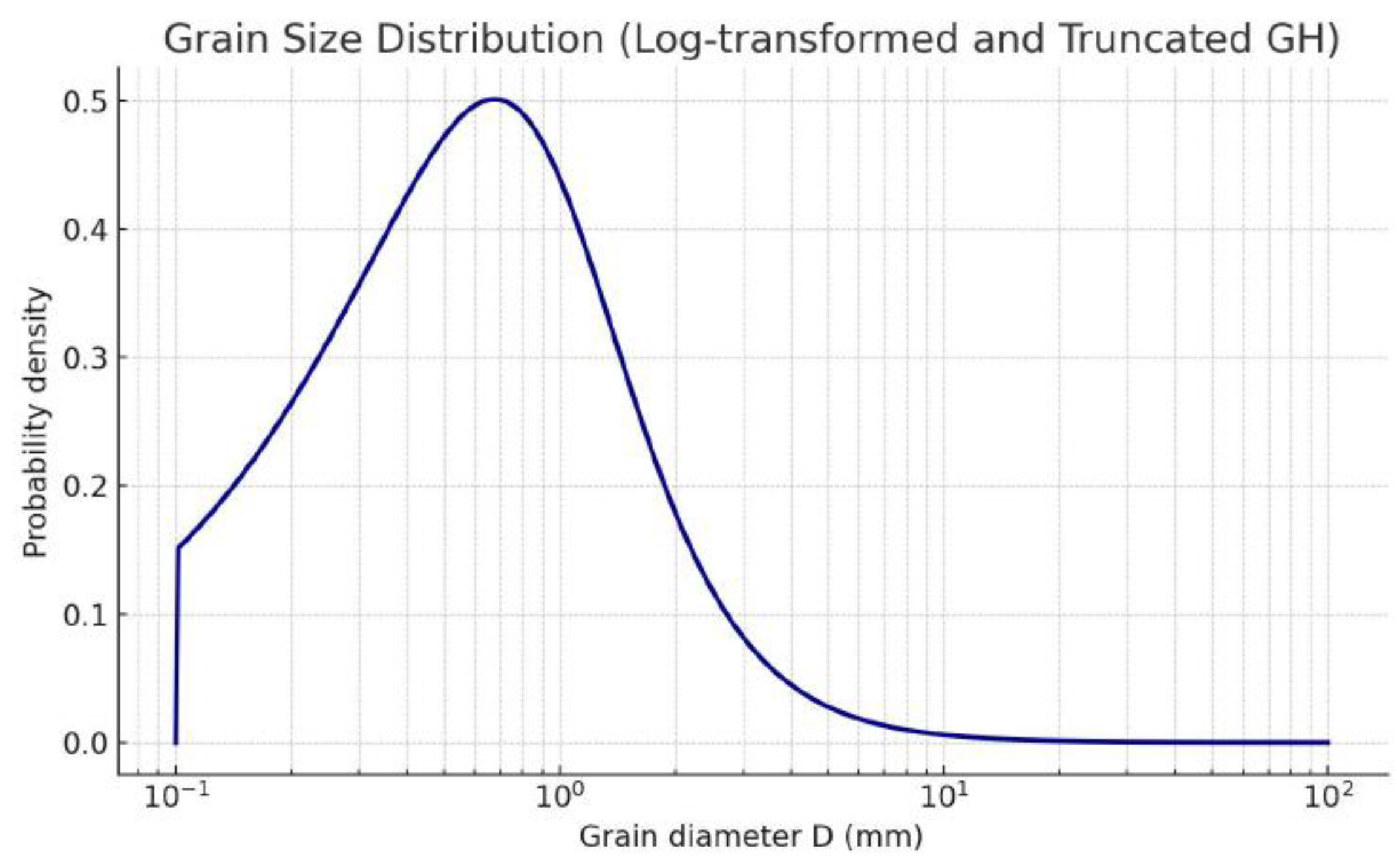
Figure 2.
Flowchart describing all the stages of the synthetic dataset generation.

Figure 3.
Left: each weight has a fixed value, as provided by classical backpropagation. Right: each weight is assigned a distribution, as provided by Bayes by Backprop [40].
Figure 3.
Left: each weight has a fixed value, as provided by classical backpropagation. Right: each weight is assigned a distribution, as provided by Bayes by Backprop [40].

Figure 4.
Flowchart describing the BNN framework.
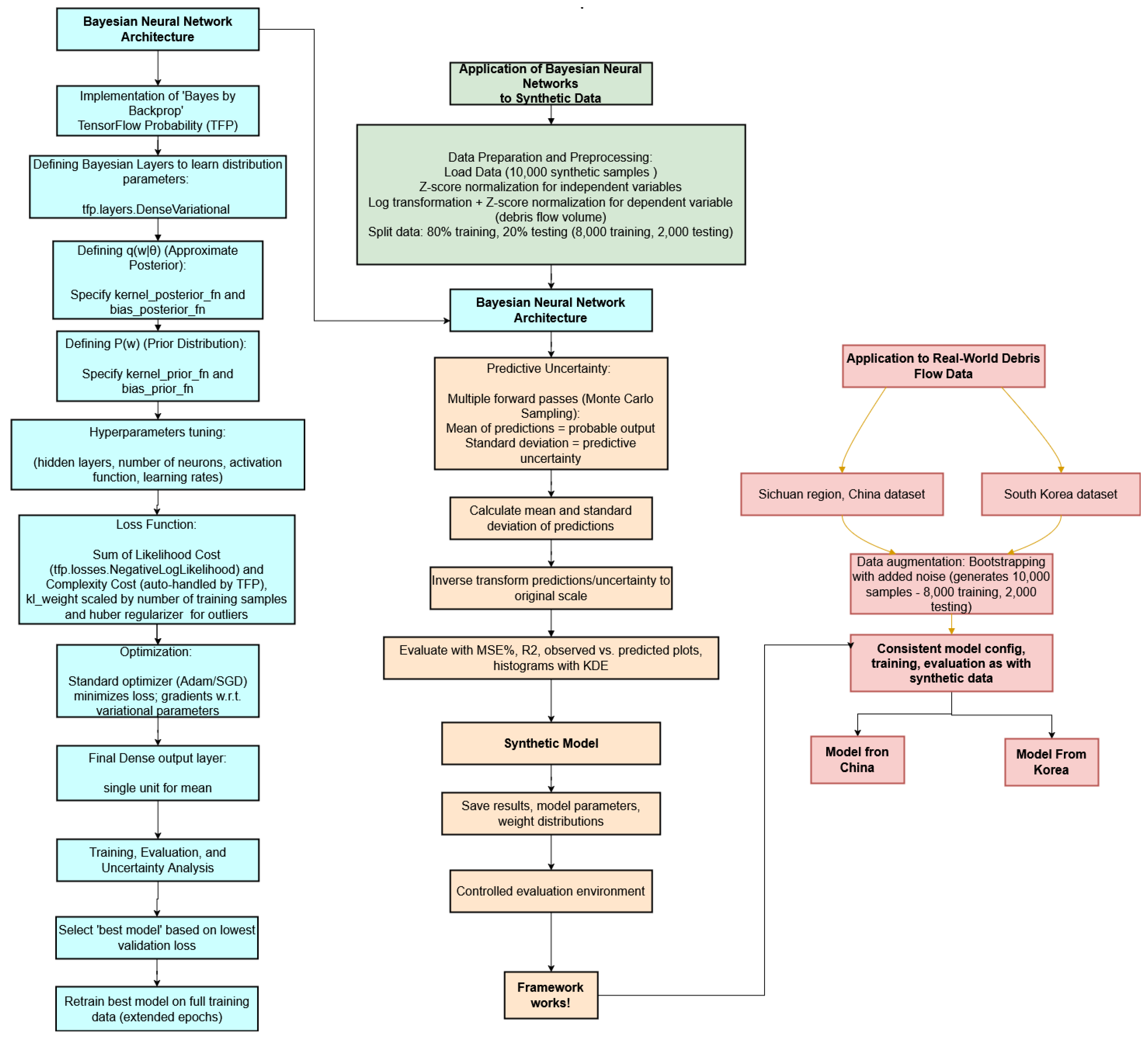
Figure 5.
Pearson Correlation Matrix of Independent Variables.
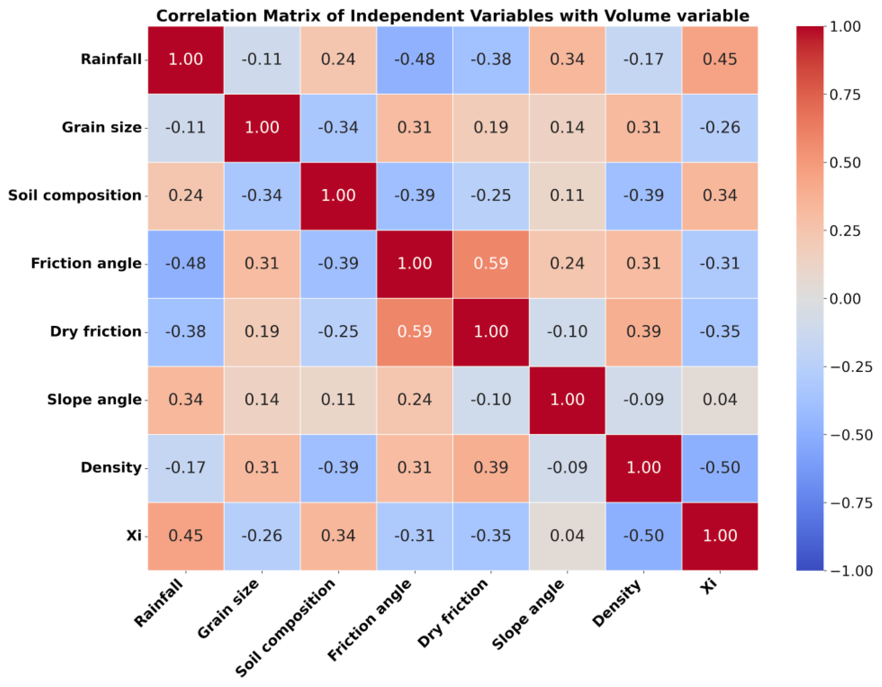
Figure 6.
Pearson Correlation Coefficients between Independent Variables and Synthetic Volume.
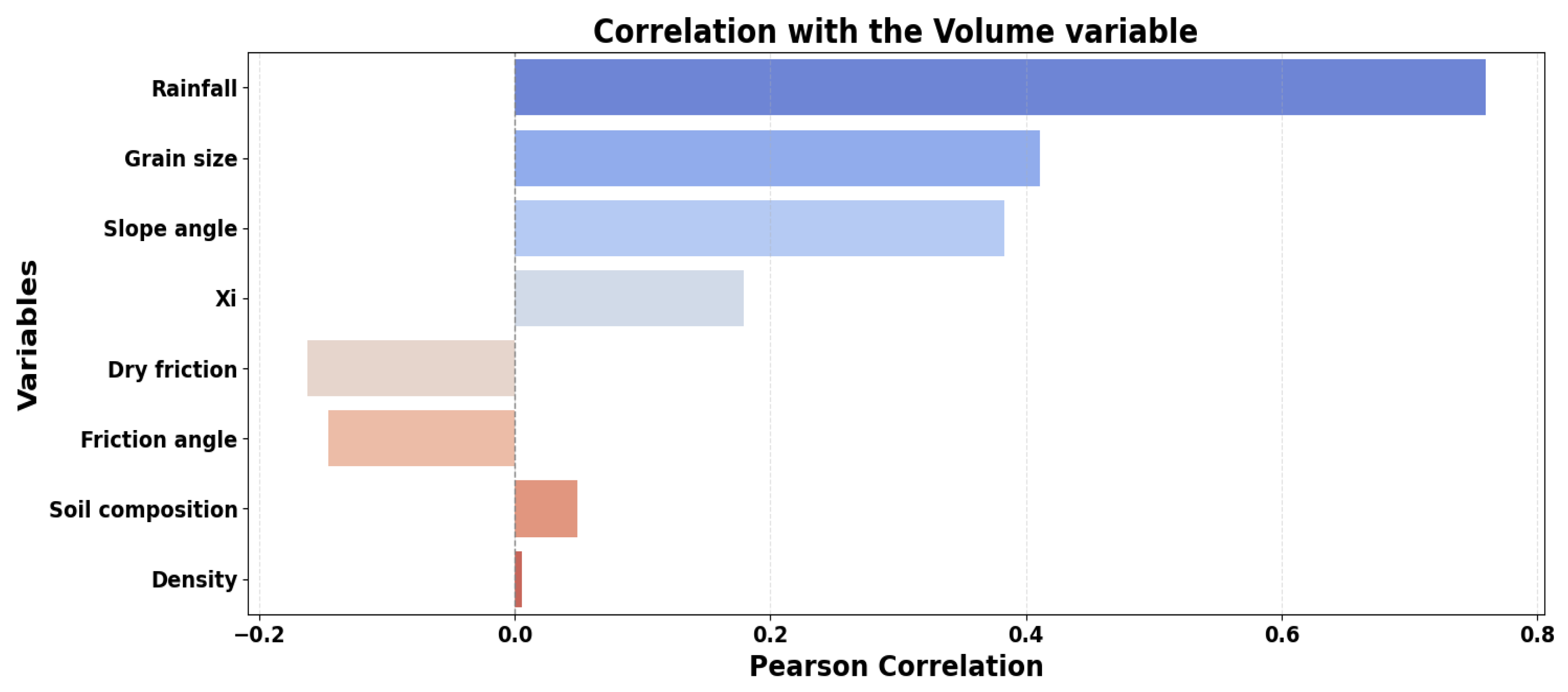
Figure 7.
Distribution of Generated debris flow Volumes.
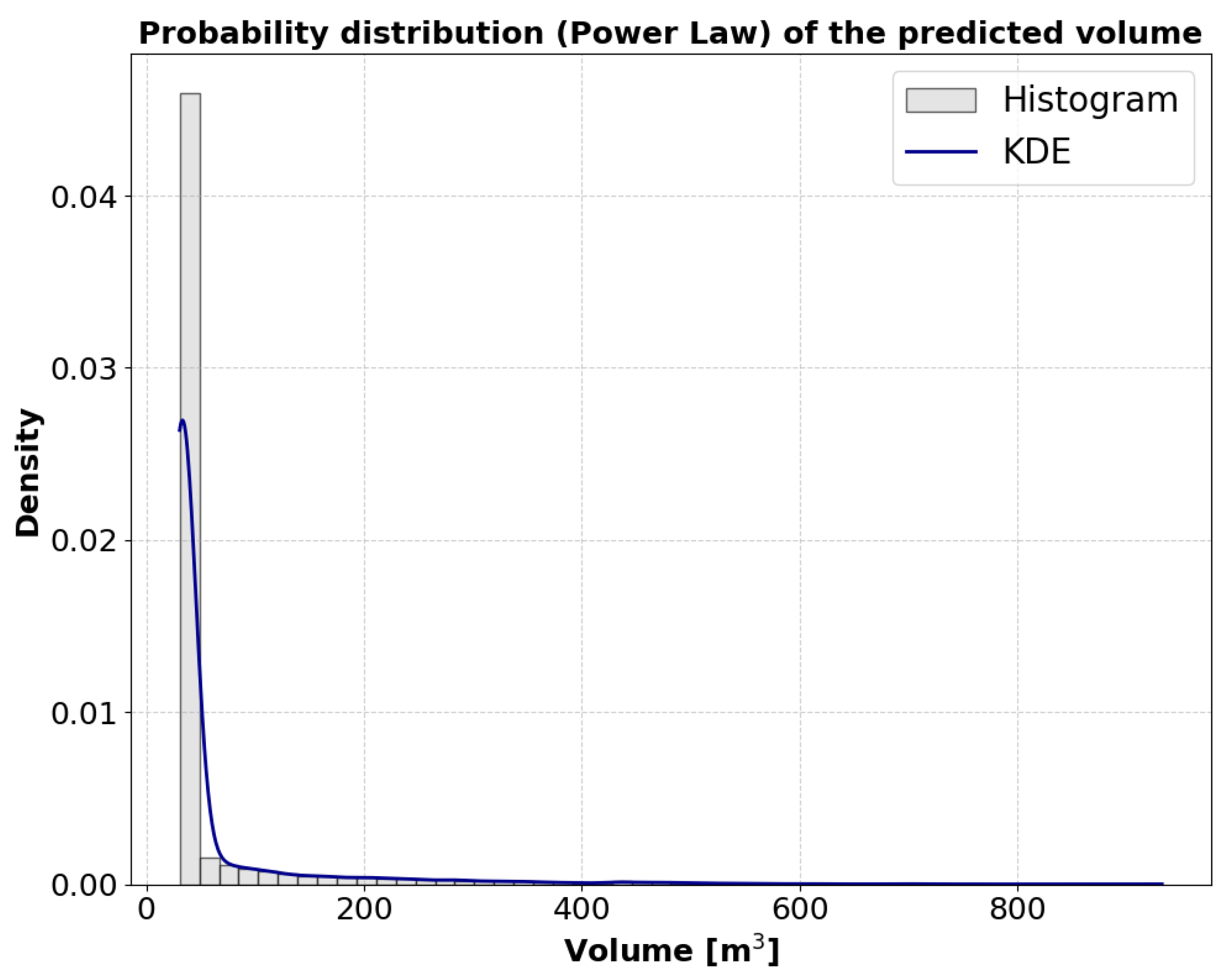
Figure 8.
Predicted vs. Volume validation values from: a) The synthetic model, b) The model from Korea and c) The model from China.
Figure 8.
Predicted vs. Volume validation values from: a) The synthetic model, b) The model from Korea and c) The model from China.
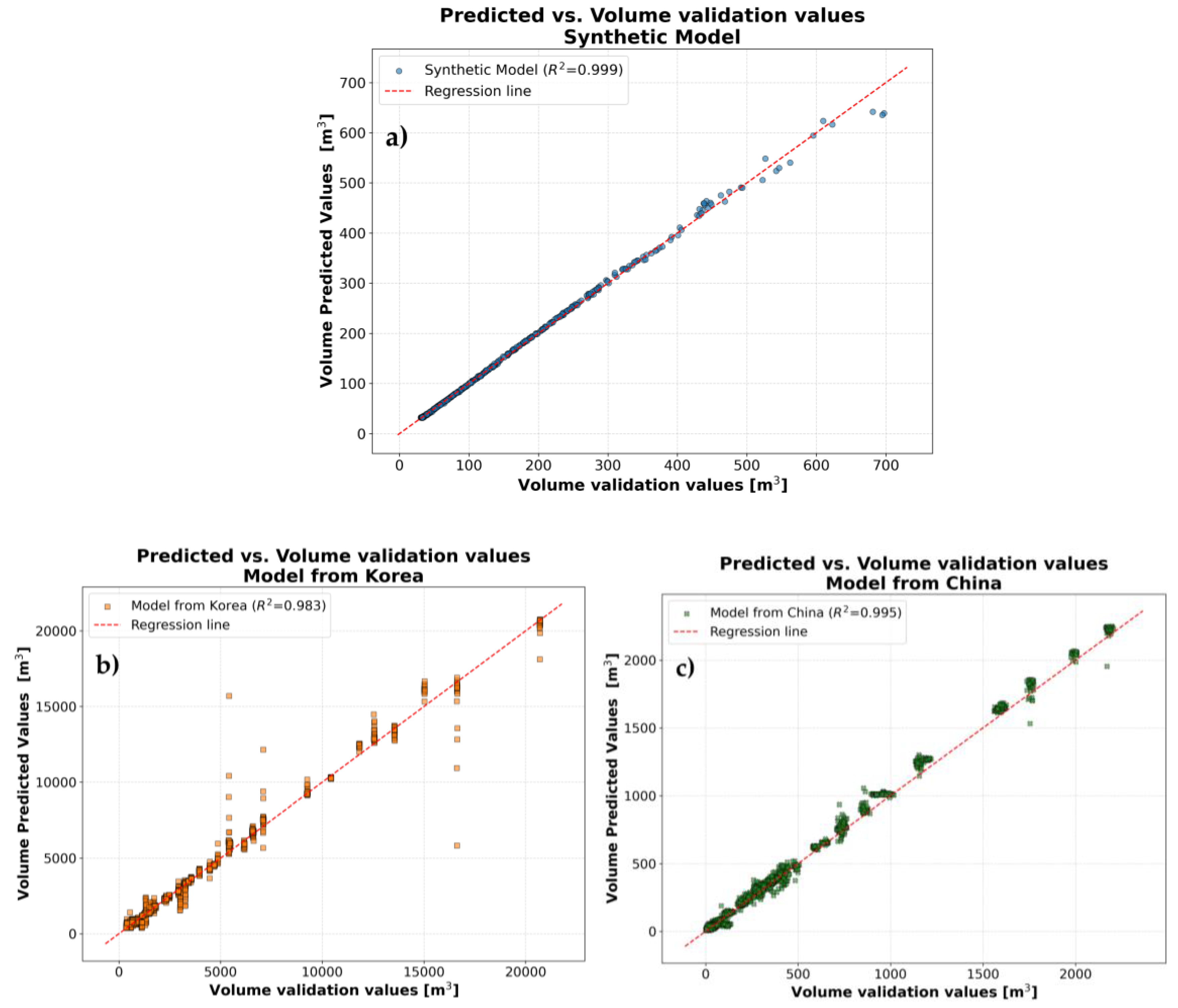
Figure 9.
Prediction Uncertainty for the: a) The synthetic model, b) The model from Korea and c) The model from China.
Figure 9.
Prediction Uncertainty for the: a) The synthetic model, b) The model from Korea and c) The model from China.
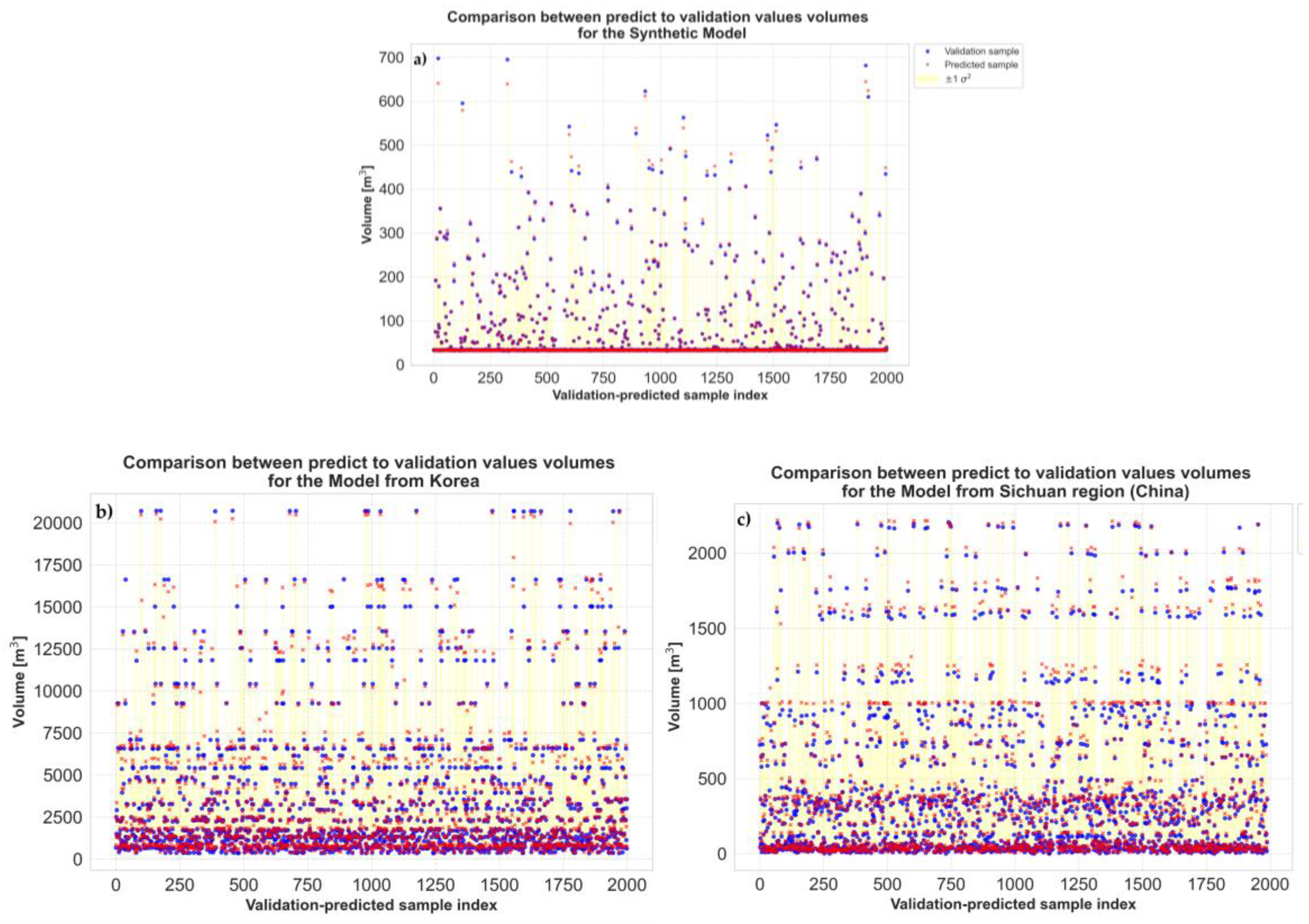
Figure 10.
Volume Distribution Characteristics for the: a) The synthetic model, b) The model from Korea and c) The model from China.
Figure 10.
Volume Distribution Characteristics for the: a) The synthetic model, b) The model from Korea and c) The model from China.
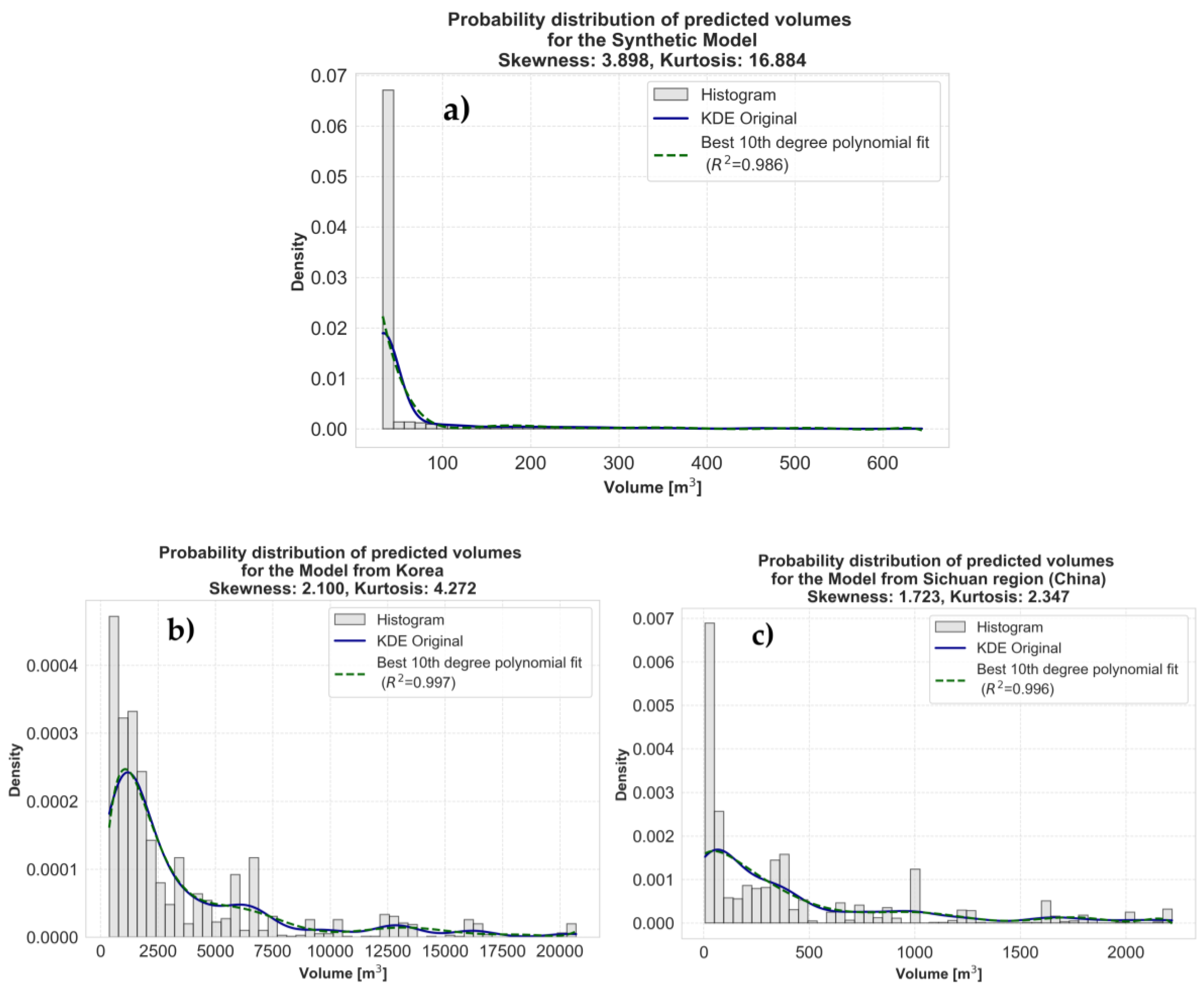
Figure 11.
Mean Relative Error (MRE) (%) values for each BNN model.
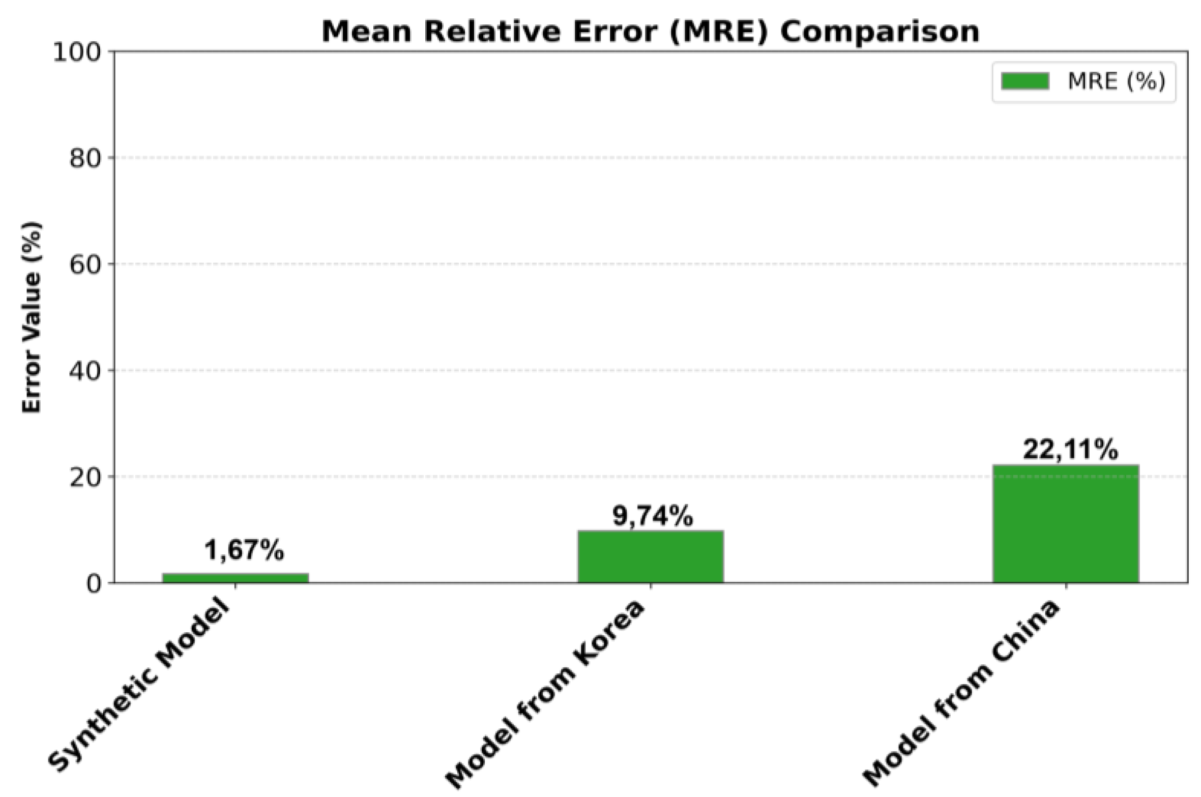
Figure 12.
Residuals plots of a) The model from China, b) The synthetic model and c) The model from Korea.
Figure 12.
Residuals plots of a) The model from China, b) The synthetic model and c) The model from Korea.
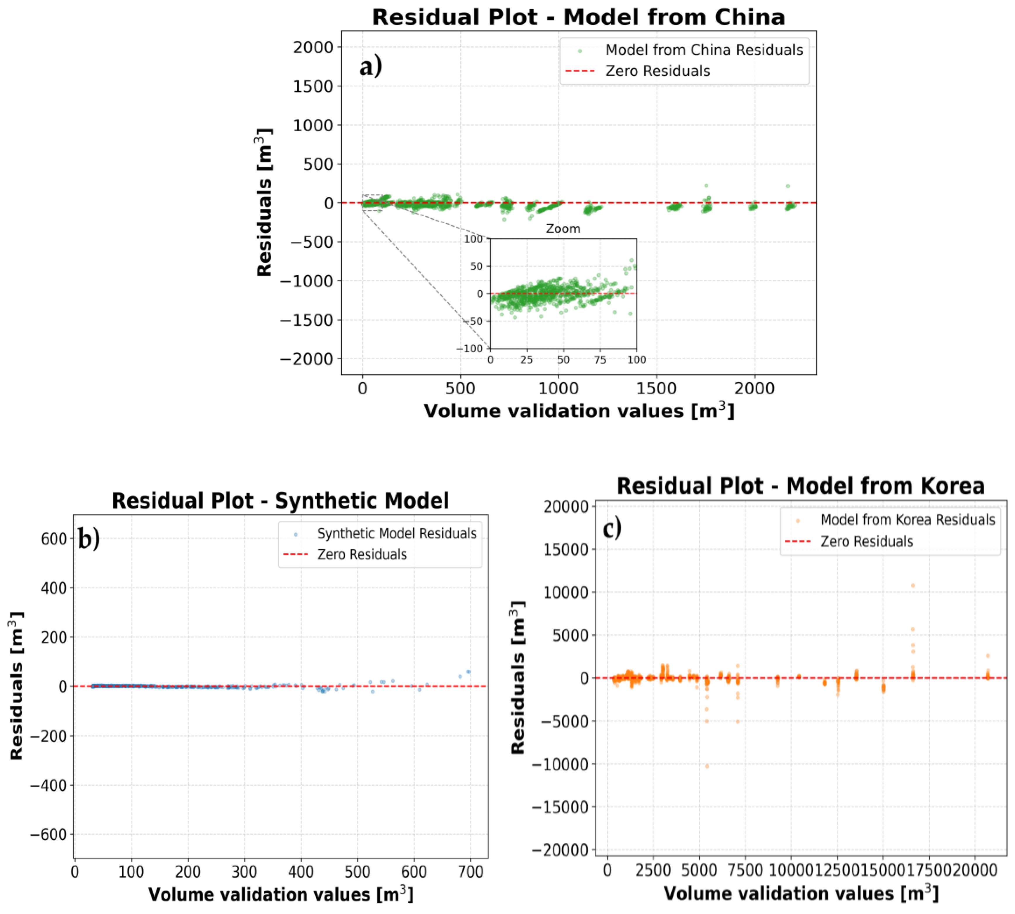

Table 1.
Predictive performance for all three BNN (Bayesian Neural Network) models.
| Model name | ||||
|---|---|---|---|---|
| Synthetic Model | 32.7 | 32.4 | 0.26 | (31.87, 32.92) |
| Model from Sichuan region (China) | 45.57 | 44.63 | 3.62 | (37.39, 51.87) |
| Model from Korea | 5445.99 | 5953.52 | 233.94 | (5485.64, 6421.41) |
Disclaimer/Publisher’s Note: The statements, opinions and data contained in all publications are solely those of the individual author(s) and contributor(s) and not of MDPI and/or the editor(s). MDPI and/or the editor(s) disclaim responsibility for any injury to people or property resulting from any ideas, methods, instructions or products referred to in the content. |
© 2025 by the authors. Licensee MDPI, Basel, Switzerland. This article is an open access article distributed under the terms and conditions of the Creative Commons Attribution (CC BY) license (http://creativecommons.org/licenses/by/4.0/).
Copyright: This open access article is published under a Creative Commons CC BY 4.0 license, which permit the free download, distribution, and reuse, provided that the author and preprint are cited in any reuse.


