
Submitted:
17 July 2025
Posted:
18 July 2025
You are already at the latest version
Abstract
Quantitative proteomics analyses rely on robust statistical methods for differential expression, impacting downstream pathway and functional enrichment. This meta-analysis investigated the influence of Hypothesis Testing Methods (HTMs) and Criteria for Biological Relevance (CBRs) on functional enrichment concordance. Five independent label-free quantitative proteomics datasets were reanalyzed using diverse frequentist (t-test, Limma, DEqMS, MSstats) and a Bayesian (rstanarm) approach. Concordance of enriched terms was assessed using Jaccard indices, categorized by four comparison types: Intra-HTM_FC_CBR, Intra-HTM_Bayes_CBR, Intra-CBR_Fixed_HTM, and Inter-HTM_Inter_CBR. Results showed highly significant differences in Jaccard similarity distributions among comparison types (Kruskal-Wallis p = 5e-04). “Intra-HTM_FC_CBR” exhibited the highest consistency, indicating minor HTM influence when using FC-based CBR. “Intra-CBR_Fixed_HTM” also maintained high concordance, suggesting robust agreement between FC and Bayesian CBRs when HTM is fixed. Conversely, “Intra-HTM_Bayes_CBR” and “Inter-HTM_Inter-CBR” showed the lowest consistency, highlighting the critical impact of Bayesian method choice and mixed comparisons on functional overlaps, particularly for Gene Ontology terms. KEGG pathways displayed more uniform, method-insensitive concordance. Sensitivity analysis confirmed the robustness of these findings. This study underscores that analytical choices profoundly influence functional enrichment outcomes, emphasizing the need for transparency and careful consideration in proteomics research to ensure reproducibility.
Keywords:
proteomics
; meta-analysis
; functional enrichment
; statistical methods
; reproducibility
1. Introduction
The “omics” era has revolutionized our understanding of biological systems, with quantitative proteomics emerging as an indispensable tool for unraveling cellular complexity, identifying biomarkers, and understanding pathology [1]. Mass spectrometry (MS)-based approaches are now the gold standard for large-scale protein identification and quantification. Among these, “label-free” quantification is a widely adopted strategy. Unlike isotopic or chemical labeling methods, it infers relative protein abundance directly from peptide ion signal intensity in the mass spectrometer. Its appeal lies in experimental simplicity, lower cost, and ability to compare multiple samples without multiplexing limitations [2]. This makes it ideal for high-throughput studies and extensive cohorts where sample integrity and efficiency are paramount. However, label-free quantification faces challenges. The precision and accuracy of peptide and protein quantification are highly dependent on numerous factors that introduce variability, affecting the reliability of biological conclusions [3]. Identifying and managing these parameters that can bias “biological reality” is crucial for obtaining meaningful and reliable results [4].
Variability originates from multiple stages. The pre-analytical stage is critical; sample type, quality and protein lysis/extraction methods significantly influence recovery and representativeness. Different extraction protocols, for instance, often yield low overlap in identified proteins due to selective solubilization, leading to biased profiles [5]. At the protein level, intrinsic characteristics like size, hydrophobicity, and post-translational modifications (PTMs) impact proteolytic digestion, solubility, and ionization efficiency. Peptide amino acid sequence also directly influences fragmentation and thus identification/quantification efficiency [6]. The instrumental stage influences by ionization efficiency and peptide ion mobility, among others. Optimization of mass spectrometer acquisition parameters (e.g., injection time, resolution, collision energy), co-elution, interference, and the quality/stability of the liquid chromatogram are also crucial [7,8]. Poor chromatographic reproducibility or high background noise severely compromise accurate peptide quantification.
After mass spectra acquisition, bioinformatic decisions profoundly alter results [9]. The choice of protein sequence database and its comprehensiveness is fundamental since an incomplete database leads to missed protein identifications. Customized databases are increasingly vital in proteogenomics, improving identification rates for organisms with incomplete genomes or specific genetic variants [10]. Databases should be complete, up-to-date, and include relevant isoforms and known variations. Search parameters in engines are equally decisive, based on enzymatic digestion (e.g., trypsin), PTMs, and expected mass errors [11]. Strict mass tolerances can omit valid identifications, while lax ones increase false positives. These parameters directly affect peptide detection, identification, and subsequent protein quantification. Mass spectrometry search engines (e.g., Mascot, Sequest, Proteome Discoverer, MaxQuant, Comet/X! Tandem) use distinct algorithms. While often yielding similar results, they differ in sensitivity and specificity, particularly for low-abundance or complex peptides [12]. Engine choice and parameter optimization influence PSM (Peptide-Spectrum Match) identification quantity and quality. Later, peptide-to-protein inference is a non-trivial next step, requiring critical decisions to avoid protein over-identification. It involves grouping PSMs corresponding to unique peptides to infer protein presence, in this sense, proteotypic peptides are crucial for unambiguous protein identification [6]. Parsimony principles and handling shared peptides among multiple proteins are key, often forming inferred protein groups. Setting FDR (False Discovery Rate) thresholds, typically 1% at peptide and/or protein level, is critical for controlling false positives and ensuring identification confidence [13].
Quantitative intensity data derived from PSMs require normalization to correct for technical variability [14]. Various methods exist for intra-replicate (e.g., total chromatogram intensity) and inter-replicate (e.g., median of total peptide intensities, quantile normalization) correction [15]. More sophisticated methods like LOESS or VSN normalize for variance-intensity dependencies [16]. Label-free specific methods like iBAQ and LFQ (in MaxQuant) perform internal normalizations across replicates [17,18]. The choice of normalization significantly impacts downstream results and the detection of biological changes [19].
Once reached, determining significantly changing proteins requires careful experimental design and appropriate statistical approaches for differential expression analysis [20]. Designs range from simple two-group comparisons to complex multifactorial or time-series experiments (Table 1). While conventional parametric methods like Student’s t-test and ANOVA are widely used [21], their assumptions (normal distribution, homoscedasticity, independence) are often violated in proteomics due to variability, missing values, and heterogeneous measurement error [22,23,24]. These classical methods limit statistical power and increase false positive/negative rates, especially in low-replication designs.
More robust alternatives address these limitations. limma performs moderated t-tests using empirical Bayes shrinkage, improving variance stability with low replicates [25]. DEqMS models protein-level variance dependence on identified peptides for precise estimates [26]. Bayesian methods (e.g., BDiffProt, BNIH) encode uncertainty and incorporate prior information, improving false discovery rate control and effect size estimation under non-normal conditions [22,27]. For longitudinal and multifactorial designs, linear mixed-effects models (MSstats) control for intra-subject correlation, repeated measurements, and batch effects [30]. These models, combined with variance moderation (limma, DEqMS), outperform classical methods in high-dimensional data with missing values or low replication [23,31]. Beyond statistical significance, biological relevance must be evaluated. While p-values indicate probability, effect size or Fold Change (FC) quantifies the magnitude of difference, directly indicating biological relevance [32]. Bayesian approaches offer direct inference about effect magnitude and the probability of biologically relevant differential expression, often using a Null Interval of Relevance for more intuitive interpretation [27].
The quantitative proteomics workflow lead to the performance of enrichment analyses to transform data into interpretable biological knowledge. These analyses identify disproportionately represented biological functions, processes, or pathways within lists of quantitatively changed proteins by integrating proteomic information with databases like GO, KEGG, and Reactome. This provides a high-level view of underlying molecular mechanisms. The robustness of enrichment results could be intrinsically linked to methodological decisions made throughout the proteomic workflow. Variability from sample preparation, data acquisition, normalization, missing value imputation, and differential expression analysis propagates, could affect input protein lists for enrichment and thus pathway interpretation. Understanding factors biasing or affecting enrichment consistency is essential for reliable biological conclusions. This study precisely addresses this fundamental need. Through a meta-analysis using the Jaccard similarity coefficient on real proteomic datasets, we aim to quantify and understand how different methodological decisions influence the robustness and reproducibility of pathway enrichment results. This approach will empirically illuminate how selections within the quantitative proteomics bioinformatics pipeline directly affect biological interpretation, providing a basis for optimizing workflows and enhancing confidence in biological inferences.
2. Materials and Methods
2.1. Dataset Selection
Five publicly available mass spectrometry (MS) proteomic works (referred to as Works 1–5) were selected for this study. Works 1, 2, and 3 were chosen randomly based on three criteria: their acquisition using an Orbitrap Fusion mass spectrometer, utilization of data-dependent acquisition (DDA) mode, and prior publication in peer-reviewed journals. Works 4 and 5 were selected from a previously published work by our research group, adhering to the same criteria. From each work, specific RAW files were obtained to perform pairwise comparisons. Information for each work is detailed below:
- Work 1 (ProteomeXchange: PXD051640) originated from a study on brown adipose tissue and liver in a cold-exposed cardiometabolic mouse model [33]. The protein database used for identification was Mus musculus (C57BL/6J) (UP000000589).
- Work 2 (ProteomeXchange: PXD041209) investigated the Escherichia coli protein acetylome under three growth conditions [34]. Protein identification relied on the Escherichia coli K12 (UP000000625) protein database.
- Work 3 (ProteomeXchange: PXD019139) explored quantitative proteome and PTMome responses in Arabidopsis thaliana roots to osmotic and salinity stress [35]. The corresponding protein database was Arabidopsis thaliana (UP000006548).
- Works 4 and 5 (ProteomeXchange: PXD034112) were derived from a comprehensive study on biological nitrogen fixation and phosphorus mobilization in Azotobacter chroococcum NCIMB 8003 [36]. The protein database for these works was UP000068210.
The files were analyzed in MaxQuant, using the parameters specified in Table S1.
2.2. Differential Abundance Analysis
Data processing and statistical analyses were primarily conducted using R (version 4.5.0) [37] within the RStudio 2025.05.0 environment, leveraging various specialized packages. The initial input for differential abundance analysis consisted of the proteinGroups.txt and evidence.txt files, which are standard outputs from the MaxQuant processing. As a crucial data preparation step (Script 1), contaminants, proteins identified by only one unique peptide, and proteins from the decoy database were filtered out from the proteinGroups.txt file. The resulting filtered dataset, named proteinGroups_filtered.txt, was then used as the primary input for most downstream statistical analyses. For all analyses, iBAQ normalized intensity data were utilized, and all selected statistical methods were robustly designed to accommodate the presence of missing values. Six distinct hypothesis testing methods (HTMs) were applied to these prepared datasets (Script 2):
- Student’s and Welch’s t-tests: Performed on the base-2 logarithm of protein intensity data to compare means between two conditions. Both Student’s t-test (assuming equal variances) and Welch’s t-test (not assuming equal variances) were conducted using base R functions.
- Limma: The limma R package [25,38] was used to fit a linear model to log2-transformed protein intensity data. This method employs empirical Bayes moderation to ‘borrow information’ across proteins, enhancing statistical power and stabilizing variance estimates, particularly critical in experiments with low biological replicates.
- DEqMS: The DEqMS R package [26] was employed, extending the limma framework by incorporating peptide count information to refine variance estimation in differential protein abundance analysis. It leverages the observation that proteins identified with more peptide-spectrum matches (PSMs) yield more reliable intensity measurements, leading to improved statistical power.
- MSstats: The MSstats R package [30] is specifically designed for quantitative mass spectrometry data. Uniquely among these methods, MSstats requires the original proteinGroups.txt file (not the filtered version) along with the evidence.txt file as input. Data was pre-processed using the dataProcess function in MSstats, and group comparisons were performed using linear mixed-effects models. This approach accounts for various sources of variability (e.g., biological/technical replicates, batch effects) by explicitly modeling them as random effects, thus providing robust variance estimates and increased statistical power.
- Bayesian Analysis: Differential protein abundance was also assessed using a Bayesian framework, implemented with the rstanarm R package [39]. This package provides an interface to Stan for Hamiltonian Monte Carlo (HMC) sampling. For each protein, a Bayesian linear regression model was fitted to the log2-transformed intensity data, utilizing the experimental condition as predictor. Model fitting employed four Markov Chain Monte Carlo (MCMC) chains with 4000 iterations (including 2000 warm-up iterations) and an adapt_delta of 0.99. Convergence of the chains was rigorously monitored using Rhat values (ideally ≤1.01) and effective sample size (ESS, ideally ≥200). This probabilistic approach yields full posterior distributions for the model parameters, which enables direct statements about effect sizes and their associated uncertainties. Weakly informative priors were incorporated to regularize parameter estimates and enhance model stability, particularly beneficial for proteins with limited measurements [40,41].
For all frequentist methods (Student’s t-test, Welch’s t-test, limma, and DEqMS), p-values were adjusted for multiple testing using the Benjamini-Hochberg (BH) method to control the false discovery rate. Proteins with an adjusted p-value ≤0.05 were considered significantly differentially abundant. For the Bayesian method, significance was determined by calculating the posterior probability that the effect size (log2FC) exceeded a predefined threshold of biological relevance (1), with proteins having a posterior probability ≥0.95 considered differentially abundant.
To provide a comprehensive overview of the differential abundance analysis results, several types of plots were generated for each pairwise comparison (Script 2): bar plots (using the ggplot2 package) visualizing the total number of significant proteins identified by each method; UpSet plots (using the UpSetR package, [42]) representing the intersections and unique sets of significant proteins across different methods, complemented by tabular summaries of these intersections; and density plots of −log10(adjusted p-value) (using ggplot2) to assess overall trends in p-value distributions from frequentist methods, including a vertical line for the significance cutoff.
2.3. Biological Relevance Filtering and Overlap Analysis
To identify proteins with significant biological relevance beyond mere statistical significance, two distinct criteria for biological relevance (CBRs) were applied to the initial results of differential abundance analysis (Script 3). The first criterion, Fold Change (FC) Filtering, was applied to proteins statistically identified as differentially abundant by the frequentist methods (t-Student, t-Welch, limma, DEqMS, MSstats). A protein was considered biologically relevant if its absolute log2 Fold Change (∣log2FC∣) was greater than or equal to 1. The second criterion, Bayesian Biological Relevance Filtering, employed the previously described Bayesian linear modeling approach. After the initial hypothesis testing, for each protein, a Bayesian linear model (fitted using the rstanarm R package; [39], with the MCMC parameters and convergence diagnostics as detailed above) was utilized. A protein was deemed biologically relevant by this criterion if the absolute mean of its posterior log2 Fold Change (∣log2FC∣) was ≥1 and the probability of this log2 Fold Change exceeding an absolute threshold of 1 (P(∣posterior log2FC∣≥1)) was ≥0.
To understand the agreement and unique contributions of each filtering strategy, intersection analysis was performed using UpSet plots [42]. For each statistical method, three sets of proteins were defined: “Originals” (statistically significant proteins from the HTMs), “FC” (proteins from the “Originals” set also meeting the Fold Change CBR), and “Bayes” (proteins from the “Originals” set also meeting the Bayesian CBR). These sets of protein identifiers were used as input for the UpSetR package in R. UpSet plots were generated to visualize the size of unique sets and all possible intersections.
2.4. Segregation and Functional Enrichment Analysis
Following the HTM analysis and CBR filtering, proteins were classified as up- or down-regulated based on their log2 FC values and the respective statistical or biological relevance thresholds (Script 4). For each HTM and CBR, separate lists of up-regulated and down-regulated protein identifications (Protein.IDs) were generated. It is important to note that while the res_bayes method originates from Bayesian inference, its results for biological relevance were also considered under the Fold Change criterion for specific downstream applications.
Functional enrichment analysis was performed using ClueGO (v2.5.9) [43] within Cytoscape (v3.10.0) [44]. For each set of upregulated and downregulated proteins identified, Gene Ontology (GO) terms (Biological Process and Molecular Function) and KEGG pathways, when possible, were interrogated. The enrichment analysis relied on a two-sided hypergeometric test, with resulting p-values corrected for multiple testing using the Benjamini-Hochberg method. Only terms with a corrected p-value <0.05 were considered significant. To reduce redundancy and improve interpretability, functionally related terms were grouped based on their kappa score using the GO Term Fusion option, and the resulting networks were visualized based on the overlap of associated genes.
2.5. Jaccard Analysis of Individual Works
To systematically evaluate the impact of HTMs and CBRs on the consistency of functional enrichment outcomes within individual quantitative proteomics datasets, % associated genes of each upregulated and downregulated datasets from each HTM and CBR frameworks were used to analyze the similarity (Script 5). Then, the similarity between these lists of enriched terms was quantitatively assessed using the Jaccard Index (J(A,B)=∣A∪B∣∣A∩B∣) [45]. Jaccard similarity indices were rigorously categorized based on the nature of the combined HTM and CBR as follows, mirroring the scheme implemented in our analysis scripts:
• Intra-HTM_FC_CBR: Comparisons between different HTMs where the CBR was consistently Fold Change-based (e.g., deqms_FC vs. limma_FC). This category assesses the variability introduced solely by the choice of HTM when a fixed FC relevance criterion is applied.
• Intra-HTM_Bayes_CBR: Comparisons between different HTMs where the CBR was consistently Bayesian posterior probability-based (e.g., deqms_bayes vs. limma_bayes). This category assesses the variability introduced solely by the choice of HTM when a Bayesian relevance criterion is applied.
• Intra-CBR_Fixed_HTM: Comparisons between the two different CBRs (Fold Change-based vs. Bayesian posterior probability-based) where the HTM was kept constant (e.g., tstudent_FC vs. tstudent_bayes). This category directly evaluates the influence of the biological relevance criterion itself, controlling for the HTM.
• Inter-HTM_Inter-CBR: Comparisons between combinations where both the HTM and the CBR differed (e.g., tstudent_FC vs. limma_bayes). This category represents the cumulative variability from changing both methodological aspects.
For each individual “Work” and for each direction of regulation (up/down), a non-parametric Kruskal-Wallis H-test (p<0.05) was performed to assess overall differences in Jaccard index distributions across these defined comparison types. If significance was detected, post-hoc Dunn’s tests with Bonferroni correction [46] were performed to identify specific pairs of groups with significantly different Jaccard index distributions.
2.6. Meta-Analysis
A comprehensive meta-analysis was performed to evaluate the consistency of biological enrichment results across various quantitative proteomics datasets and statistical methodologies (Script 6). The pre-computed and categorized Jaccard similarity indices from each individual “Work”, as described in the previous section, served as the foundational data for this meta-analysis. This approach ensured the ecological validity of our meta-analysis beyond controlled benchmark scenarios [47,48].
For integration, raw ontology names, which sometimes included dataset-specific suffixes or dates, were systematically standardized to their core functional categories (e.g., “GO_BiologicalProcess”, “GO_MolecularFunction”, “KEGG”). All extracted Jaccard indices from all “Works” were then transformed using the arcsin square root transformation (arcsin(√J)) to improve normality and homogeneity of variance, a common practice for proportional data. These transformed indices were combined into a single, comprehensive dataset, along with metadata detailing the original Work, normalized ontology, direction of regulation (up/down), and their specific methodological comparison category.
Statistical analysis for the meta-analysis was conducted using the non-parametric Kruskal-Wallis test to assess overall differences in transformed Jaccard index distributions across the comparison types. This was followed by Dunn’s post-hoc test with Bonferroni correction for pairwise comparisons when global significance was observed. The robustness and consistency of the overall findings were further evaluated through a sensitivity analysis, where the Kruskal-Wallis test was re-run by systematically excluding one ‘Work’ at a time from the meta-analysis dataset.
3. Results and Discussion
Quantitative proteomics experiments aim to identify and quantify changes in protein abundance across different biological conditions. A critical downstream step involves pathway and functional enrichment analysis, which translates lists of differentially expressed proteins into biologically meaningful insights. However, the statistical methods employed for differential expression analysis can vary significantly, broadly categorized into frequentist approaches (e.g., t-tests, ANOVA, linear models) and Bayesian methods (e.g., typically incorporating prior information or empirical Bayes). The choice of method could profoundly impact the resulting list of significant proteins, consequently affecting the outcome of subsequent enrichment analyses.
In this work, five previously published quantitative proteomics independent studies (“Works”) were reanalyzed to elucidate the impact of the non-biological component of sample-to-sample comparison experiments using label-free quantitative proteomics. All were analyzed using the same parameters in MaxQuant (Table S1), thus limiting the differences to the biological parameters of the experiment itself and those derived from the statistical decisions under study. However, these parameters were also not identical to those of the original studies, which would explain possible differences with respect to them. To our knowledge, this study presents a novel meta-analytical approach by combining enrichment results from diverse real-world, independently published quantitative proteomics datasets rather than controlled benchmark datasets. This allows for a comprehensive evaluation of the relative influence of both specific HTMs and distinct CBRs on downstream biological interpretations, reflecting the variability encountered in actual research. While method benchmarking studies often utilize specially prepared datasets to validate new approaches, the use of a meta-analysis on randomly selected or pre-existing “real” datasets is less common and offers valuable insights into the generalizability and robustness of analytical choices in routine proteomics research. By analyzing the different Works, we aim to address three key questions regarding the influence of statistical methodologies on biological enrichment findings:
• Does the specific hypothesis testing method (HTM; e.g., t-Student, t-Welch, Limma, DEqMS, MSstats, Bayesian) influence the resulting biological enrichments when the criterion for biological relevance (CBR) is kept constant?
• Does the method used for determining biological relevance (CBR; Fold Change-based vs. Bayesian posterior probability-based approaches) influence the resulting biological enrichments when the hypothesis testing method (HTM) is kept constant?
• What has a greater influence on the observed biological enrichments: the specific hypothesis testing method (HTM) or the criterion for determining biological relevance (CBR)?
3.1. Protein Groups Variability
Prior to examining the differential expression results, it is crucial to understand the inherent variability within each experimental condition (Table 2). The median coefficient of variation (CV) offers insights into the reproducibility of protein quantification within each condition. In Works 1, 4, and 5, a notable disparity in the consistency of protein quantification between conditions is observed. Specifically, in these Works, Cond2 exhibits a considerably higher median CV than Cond1. For Works 4 and 5, the variability in Cond2 is particularly pronounced, significantly exceeding that observed in Cond1. It is important to note that, for these Work, Cond2 was derived from the same raw files, suggesting that these differences in CV primarily stem from the impact of normalization strategies applied across different replicates on the final observed protein quantification. High CVs can indicate greater biological variability, technical noise, or a combination of both. Conversely, Work3 shows relatively low and similar median CVs for both conditions, indicating more consistent and reproducible protein quantification. Work2 also presents relatively high CVs for both conditions, but with a less dramatic difference between them. The standard deviation (SD) of the absolute log2 fold change (|Log2FC|) provides a measure of the spread of the observed changes in protein abundance between the two conditions. Higher SD values indicate a wider range of fold changes, suggesting more diverse responses to the experimental manipulation. The |Log2FC| SD is relatively low in Work1 (1.06) compared to the other Works, indicating a more uniform response. In contrast, Works 2, 4, and 5 exhibit higher |Log2FC| SD values (3.94, 3.59, and 3.9, respectively), suggesting more heterogeneous protein abundance changes. Work3 shows a moderate |Log2FC| SD of 2.73.
Levene’s test assesses the equality of variances between the two conditions. A p-value greater than 0.05 indicates no significant evidence to reject the null hypothesis of equal variances, while a p-value less than or equal to 0.05 suggests that the variances may be different. In our data, Works 2 and 3 have Levene’s test p-values greater than 0.05 (0.9313 and 0.1317, respectively), suggesting that the variances between the two conditions are not significantly different. However, Works 1, 4, and 5 have p-values lower than 0.05 (0, 0.0117, and 0.001, respectively), indicating significant differences in variances between the conditions, which should be considered when selecting appropriate statistical methods for differential expression analysis. Methods that assume equal variances may not be appropriate for these datasets. This analysis of protein group variability, the spread of fold changes, and variance equality provides important context for interpreting the subsequent differential expression results. Datasets with higher CVs or unequal variances between conditions may require more robust statistical methods or more careful interpretation of the results.
3.2. Differential Expression Analysis and Impact of Hypothesis Testing Methods
The input data for this study originated from a protein groups file (proteinGroups.txt) and an evidence file (evidence.txt) obtained from mass spectrometry experiments. For differential abundance analysis, we applied six different statistical methods, five frequentists: t-test [52], t-test with Welch’s correction [53], limma [38], DEqMS [26], MSstats [30]; and a Bayesian approach utilizing rstanarm [39,54]. It is indeed plausible to state that brms was initially considered for the Bayesian analysis but proved computationally unfeasible for routine use, leading to the adoption of rstanarm, with higher efficiency for standard generalized linear models (GLMs) due it frequently leverages pre-compiled Stan code, significantly reducing the compilation time often required by brms for each model specification [54,55]. Nevertheless, both packages are widely recognized and applied in quantitative proteomics for differential expression analysis due to their ability to provide full posterior distributions for parameters of interest, quantify uncertainty, and incorporate prior knowledge, which can be particularly advantageous with limited biological replicates [56]. The Bayesian method implemented via rstanarm was employed for both hypothesis testing and, in a single step, the determination of statistical significance, which inherently accounts for biological relevance through its probabilistic framework. Differential expression analysis was performed using each of these six methods on the respective input data, and the resulting lists of differentially abundant proteins were compared based on adjusted p-values.
The number of identified differentially expressed proteins (DEPs) varied considerably across the six statistical methods (Bayesian, DEqMS, Limma, MSstats, t-Student, and t-Welch) and the five distinct workflows (W1-W5), as depicted in Figure 1A. A general pattern observed in Panel A is that MSstats consistently identifies a larger number of DEPs across most workflows compared to other methods, suggesting higher sensitivity or a less stringent filtering of significance. Conversely, the Bayesian method often yields a more conservative number of DEPs, particularly noticeable in workflows where other methods report a high count. Limma and DEqMS tend to show intermediate numbers, while t-Student and t-Welch results are also variable. This variability highlights the dependency of DEP lists on the chosen statistical approach, a well-documented challenge in proteomic data analysis. The UpSet plots in Figure 1B provide crucial insights into the overlap and unique identifications among the methods for each workflow. A key pattern emerging from Panel B, particularly evident in workflows with a higher overall number of DEPs (e.g., Work1, Work4), is that while a substantial core set of proteins is often identified by multiple methods, indicating high confidence, there are also considerable numbers of DEPs unique to one or a few specific methods. This observation reinforces that different statistical models emphasize distinct aspects of the data, potentially due to variations in assumptions regarding variance estimation or outlier handling [56]. For instance, methods showing higher individual DEP counts (like MSstats) also tend to contribute a larger number of unique DEPs, suggesting their sensitivity might capture a broader range of subtle changes or, conversely, a higher rate of false positives if not adequately controlled. Thus, the choice of HTM profoundly influences the sheer volume of proteins deemed significant, a critical factor for downstream biological interpretation.
The distribution of adjusted p-values, as presented in Figure S1, provides further insights into the behavior and sensitivity of the six statistical methods across the five Works. A sharp peak near the origin (low negative log-base-10 adjusted p-value) is consistently observed, representing non-significant proteins, as expected. Crucially, the right tail of these distributions, corresponding to statistically DEPs, varies notably. MSstats, consistent with its higher DEP counts in Figure 1A, typically displays a broader distribution extending to higher negative log-base-10 adjusted p-value values (e.g., in Work1, Work4). This indicates that MSstats assigns lower adjusted p-values to more proteins, suggesting higher sensitivity, but also potentially a higher false positive rate if not carefully controlled. Conversely, methods like Bayesian, t-Student, and t-Welch show distributions more concentrated at lower negative log-base-10 adjusted p-value values, with minimal density in the right tail. This reflects their more conservative nature and lower DEP counts, as seen in Figure 1A, indicating fewer proteins meeting significance thresholds. The shape of these distributions, particularly the presence of a “spike” near the significance threshold, can indicate a method’s ability to discern true DEPs from noise [57]. While not strictly bimodal, MSstats’ shifted distribution suggests a more substantial set of low p-values. Finally, the variability in p-value distributions across workflows emphasizes the significant impact of data processing and normalization steps on statistical outcomes. In essence, Figure S1 confirms that the chosen statistical method profoundly influences the statistical evidence for differential expression, impacting the final DEP list due to varying sensitivities.
3.3. Biological Relevance in Differential Proteomics Analysis
Beyond statistical significance, the biological relevance of identified proteins is paramount for meaningful interpretation in proteomics studies. This often involves applying additional filters, such as fold change thresholds or probabilistic assessments from Bayesian analyses, to refine the list of potentially interesting proteins. Figure 2 illustrates the overlaps in significant proteins among different frequentist HTM (Student’s t-test, Welch’s t-test, Limma, DEqMS, and MSstats) after the application of these biological relevance filters across Works 1, 2, 4, and 5 (Panels A to D). Work 3 is not included in this figure due to an insufficient number of significant results after the initial statistical testing and subsequent filtering for biological relevance.
Considering the Limma method as an example we found that the ‘O’ set, representing all proteins initially significant by Limma, comprises 3630 proteins (Figure 1). From this ‘O’ set, 2311 proteins are deemed biologically relevant by the Bayesian and FC filters, and 3322 proteins (2311 + 1011) the FC filter. This detailed breakdown highlights that while some proteins exhibit robust agreement across all criteria, a significant number of proteins pass one biological relevance filter but not the other, indicating distinct filtering specificities. Meanwhile, 308 proteins didn’t surpasses any of the biological relevance (Bayesian or FC). Works 2 (B), 4 (C), and 5 (D) present more varied patterns. In Work 2, the total number of significant proteins (Set ‘O’) is considerably smaller for some methods (e.g., t-Student, t-Welch) compared to Work 1, aligning with the observations from Figure 1 regarding method sensitivity. This reduced initial set of significant proteins naturally leads to fewer proteins passing the biological relevance filters, as seen by the smaller absolute set sizes for ‘B’ and ‘FC’. Nevertheless, the previously found pattern is also observed not only in the rest of the datasets in Work1, but is quite common in all the works, thus showing that the biological relevance filter using Bayesian analysis is more restrictive than the FC. This is especially evident in work 5, where hardly any proteins with biological relevance are identified after applying the Bayesian method (only 1 is found after hypothesis testing with MSstats). Moreover, when using the Bayesian method after hypothesis testing with frequentist methods, fewer proteins with biological relevance are always found (Figure 2) than when the Bayesian method is used as both the hypothesis testing test and a method to determine biological relevance (Figure 1). This observed variability suggests that different statistical approaches, such as fold change versus Bayesian methods, may not always perfectly agree, especially when dealing with noisier datasets or more subtle biological effects. The consistency observed in certain methods stems from their robustness to common proteomics challenges like missing values and outliers. For instance, MSstats is designed to manage missingness through imputation or probabilistic modeling, while Limma’s empirical Bayes moderation stabilizes variance estimates, particularly with small sample sizes [24,30,46]. When these methods are applied to data where such issues are effectively managed, their convergence on similar significant findings underscores their reliability.
Beyond proteins passing initial filters, we investigated whether discarded proteins followed specific patterns. As anticipated from Figure 2, proteins eliminated by the Bayesian method’s filter were largely expected to include those removed by the Fold Change (FC) filter. For instance, in Work1, this general expectation held true, except for proteins discarded after using the MSstats test. In this specific case, 459 proteins were commonly discarded by both MSstats and FC filters, while 373 were uniquely eliminated by the Bayesian method, and 1,202 uniquely by the FC filter (Figure S2). This demonstrates that applying the Bayesian CBR filter not only tends to discard more proteins but also, depending on the preceding hypothesis test, the set of discarded proteins can differ significantly from those removed by the FC filter. This highlights a fundamental distinction: while FC is a purely magnitude-based filter, Bayesian methods integrate uncertainty into their relevance assessment. This provides a complementary perspective where a substantial effect size might be down-prioritized if statistical confidence is low [40]. Consequently, the selection of both the hypothesis testing method and the biological relevance criterion jointly determines the final set of relevant proteins, directly influencing downstream pathway and functional enrichment analyses.
3.4. Functional Enrichment and Similarity Profiles
Following the application of biological relevance filters to identify differentially expressed proteins, functional enrichment analyses were subsequently performed. Once significant enrichment terms were obtained, the evaluation proceeded to assess the significance of changes in these functional profiles across the different analytical methods developed. It is important to note that, while Work3 had already yielded an insufficient number of significantly distinct proteins following initial statistical testing and filtering (as discussed in the previous section), at this subsequent enrichment stage, we similarly did not find enough enriched terms for both Work2 and Work5 (encompassing lists of both upregulated and downregulated proteins), nor specifically for the downregulated proteins of Work1. Consequently, the ensuing assessment of functional enrichment and similarity profiles, as visually represented in Figure 3, focuses solely on selected data subsets from “Work1 (upregulated)” and “Work4 (up- and down-represented)”.
The Jaccard similarity distributions for Work1, across Biological Process, Molecular Function, KEGG pathways, and an “All Ontologies” aggregate, revealed significant differences. The Kruskal-Wallis rank sum test yielded a chi-squared value of 8.6305 (df = 3, p = 0.03463), indicating that the comparison types within Workflow 1 had a statistically significant, non-random impact on the observed functional similarities. This result (p < 0.05) necessitates further post-hoc analysis to pinpoint the specific differing comparison types (Dunn, 2017). Detailed pairwise Jaccard similarities, particularly for Biological Process, Molecular Function, and KEGG pathways, provide granular insights into which specific groups or comparisons drive this overall statistical significance. Tightly clustered regions of high similarity within these comparisons underscore consistent functional patterns.
For Work4, focusing on upregulated (“up”) entities, the analysis revealed highly significant differences in Jaccard similarity profiles across Biological Process, Molecular Function, and the “All Ontologies” aggregate. The Kruskal-Wallis test for “Work4_up” yielded a p-value of 2.289e-05 (chi-squared = 24.182, df = 3), strongly indicating profound impacts of comparison type on functional relationships for upregulated entities [58]. Conversely, for downregulated (“down”) entities, the “Work4_down” component, specifically within the Biological Process ontology, showed a borderline but still statistically significant difference (p = 0.04404, chi-squared = 8.0974, df = 3) (no significant enrichment results were obtained on other ontologies). This suggests that comparison types also influence functional similarity for downregulated elements, albeit less profoundly than for upregulated ones [59].
Collectively, the consistent statistical significance (p<0.05 for Work1 and Work4_down; p < 0.001 for Work4_up) from the Kruskal-Wallis tests across all analyzed workflows underscores that the methodological approach to comparison profoundly impacts Jaccard similarity measures. This highlights the critical importance of selecting appropriate comparison types in functional enrichment analyses. While summary statistics offer initial understanding, detailed pairwise relationships reveal clusters of high or low similarity, with consistently high Jaccard indices signifying shared functional characteristics and low indices indicating distinct functional roles [45]. The striking difference in significance between “up” and “down” components in Work4, with stronger significance for upregulated entities, suggests potentially more distinct and discernible functional patterns in gene activation compared to downregulation. Future investigations could benefit from post-hoc tests (e.g., Conover’s test or pairwise Wilcoxon rank sum tests with Bonferroni correction) to precisely identify specific differing comparison groups [60], and from integrating these functional similarity insights with upstream expression data or network analyses for a more comprehensive understanding.
3.5. Meta-Analysis
Finally, a meta-analysis was performed with the objective of systematically evaluating the impact of diverse statistical methodologies on the outcomes of biological enrichment analysis. This meta-analysis compiled Jaccard indices from multiple quantitative proteomics “Works,” categorizing them into four primary comparison types based on the interplay between the HTM and the CBR: “Intra-HTM_FC_CBR,” “Intra-CBR_Fixed_HTM,” “Inter-HTM_Inter-CBR,” and “Intra-HTM_Bayes_CBR.” An “Unknown” category with very few data points was also observed, representing method combinations not fitting the primary classifications; due to its sparse representation, the interpretation focuses on the four main comparison types. The distribution of Jaccard indices, both in their original and arcsin square root transformed forms, are presented in Figure 4, Panels A and B, respectively.
The arcsin square root transformation generally shifts the distribution towards a more symmetrical form, which is beneficial for statistical analyses. The results are presented both globally (across all analyzed ontologies and Works combined) and specifically for key Gene Ontology (GO) and KEGG pathway ontologies (Figure 4C and Figure 5A). The global analysis (Figure 4C) reveals a highly significant overall difference in Jaccard similarity distributions among the comparison types (Kruskal-Wallis p = 5e-04). A clear hierarchy of consistency emerges when comparing the median Jaccard indices:
• “Intra-HTM_FC_CBR” (red boxplot in Figure 4C) exhibits the highest median Jaccard indices, indicating a remarkably high degree of agreement among different frequentist HTMs (e.g., Limma, DEqMS, t-Student, t-Welch, MSstats) when identifying enriched terms using a Fold Change (FC)-based criterion for biological relevance. This suggests that within the frequentist paradigm, the specific choice of HTM has a relatively minor influence on the resulting biological enrichments.
• “Intra-CBR_Fixed_HTM” (grey boxplot in Figure 4C) shows high consistency, with its median Jaccard indices not significantly different from “Intra-HTM_FC_CBR” (p = ns). This is a pivotal finding, indicating that the consistency observed when changing the relevance criterion (from FC to Bayesian) while keeping the HTM fixed is comparable to the consistency achieved when varying HTMs solely within the FC paradigm. This challenges the initial assumption that these fundamental differences in defining relevance would lead to substantial divergence, suggesting a robust overlap in the biological terms deemed relevant by both FC and Bayesian criteria when derived from the same initial statistical assessment [45].
• “Inter-HTM_Inter-CBR” (yellow boxplot in Figure 4C) and “Intra-HTM_Bayes_CBR” (blue boxplot in Figure 4C) show similarly lower levels of consistency, with no significant difference between them (p = ns). Both are significantly lower than “Intra-HTM_FC_CBR” (p < 0.01 and p < 0.0001, respectively) and “Intra-CBR_Fixed_HTM” (p = ns for Inter vs Intra-CBR, p < 0.0001 for Intra-Bayes vs Intra-CBR). This suggests that changing HTMs within the Bayesian paradigm, or changing both HTM and CBR simultaneously, leads to similarly low consistency in enrichment results. This also implies that selecting one Bayesian method over another might be more critical for the qualitative outcome of enrichment analysis than the choice among frequentist methods.
Ontology-specific analysis (Figure 5A) largely maintains these global trends. For “GO_BiologicalProcess” (Kruskal-Wallis p = 0.033) and “GO_MolecularFunction” (Kruskal-Wallis p = 0.0019), “Intra-HTM_FC_CBR” (red) generally exhibits higher overlap, and “Intra-CBR_Fixed_HTM” (grey) often performs comparably. The lowest consistency consistently remains with “Intra-HTM_Bayes_CBR” (blue) and “Inter-HTM_Inter-CBR” (yellow) for these GO terms. However, for “KEGG” pathways (Kruskal-Wallis p = 0.038), a notable difference persists: all four comparison types exhibit relatively high and non-significantly different Jaccard indices in most pairwise comparisons (p = ns). This reinforces that for KEGG pathways, neither the specific HTM nor the CBR exerts a predominantly stronger influence on the observed enrichments, suggesting a more consolidated and less method-sensitive nature for these well-defined molecular networks [59]. This observation aligns with previous studies that report good agreement among various differential expression tools for protein quantification, especially when dealing with well-behaved data or distinct changes [56,61].
A sensitivity analysis was performed by systematically excluding one “Work” (dataset) at a time and re-running the Kruskal-Wallis test on the remaining data. Globally, when Workflow 1 or Work4_up were individually excluded, the Kruskal-Wallis p-values remained very low (close to 0). This strongly indicates that the observed global differences in Jaccard index distributions are robust and not primarily driven by these two datasets. Conversely, excluding Work4_down resulted in the Kruskal-Wallis p-value notably increasing to approximately 0.015-0.02. While still below the 0.05 significance threshold, this higher p-value suggests Work4_down has a more substantial influence on the overall statistical significance compared to Work 1 or Work4_up. These results confirm the robustness of our main findings regarding the differential consistency among comparison types, particularly with respect to Work 1 and Work4_up. However, the greater impact of Work4_down on overall significance points to a potential dataset-specific variability or an outlier effect that warrants further investigation. This implies that while broad trends exist, the precise statistical significance of methodological impacts can sometimes be influenced by individual datasets, underscoring the importance of meta-analysis for generalizability.
3.6. Conclusions and Implications
This meta-analysis represents a novel systematic approach to evaluate the impact of statistical methodologies on biological enrichment analysis outcomes by synthesizing Jaccard index data across multiple independent quantitative proteomics studies. Our comparative framework, utilizing real-world and independently sourced datasets rather than artificially constructed benchmarks, proved that depending on the choices made at different stages of the analysis, the results regarding biological enrichments can vary drastically. To begin with, we observed that the results obtained were not identical to those presented by the original authors, despite using the same raw files. This discrepancy is attributed to differences in the search and quantification process, as well as variations in the number of replicates used in the normalizations. Furthermore, it has been shown how highly variable samples compromise the tests’ ability to determine significance. Thus, reducing non-biological variability (technical variability) as well as non-controlled biological variability becomes essential. In this sense, the use of standardized protocols, the introduction of control points at key stages such as sample preparation, the collection of samples by cross-referencing physiological data, proper management of batch effects, uniform storage conditions, and an adequate number of replicates per condition have a direct positive impact on statistical power by reducing noise.
On the other hand, we observed that while specific frequentist HTMs within their paradigm yield high and consistent enrichment results (“Intra-HTM_FC_CBR”), the agreement remains high even when comparing FC-based and Bayesian-based CBRs if the underlying HTM is fixed (“Intra-CBR_Fixed_HTM”). Crucially, we showed that the consistency when varying HTMs within the Bayesian paradigm (“Intra-HTM_Bayes_CBR”), or when varying both HTM and CBR simultaneously (“Inter-HTM_Inter-CBR”), is the lowest among the groups. This implies that the choice between frequentist and Bayesian HTMs, as well as the specific Bayesian method utilized, profoundly impacts the overlap of identified terms for GO ontologies. This observation is crucial for ensuring the reproducibility and comparability of proteomics studies, as differing analytical pipelines and data processing choices can lead to divergent conclusions, sometimes even resulting in a lack of significant protein findings after hypothesis testing or an insufficient number of significant enrichments for downstream functional analyses. These findings underscore the importance of transparency in reporting statistical methods in proteomics studies and encourage researchers to consider the implications of their analytical choices on the biological interpretation of their data. The sensitivity analysis further emphasizes that while general patterns emerge, individual datasets can exert notable influence on the overall statistical significance of these methodological comparisons. For all these reasons, proteomic analysis (and omics in general) must include a cross-validation stage with techniques such as Western blot, ELISA, or targeted MS (PRM/SRM) and/or functional validation outside the proteomic framework [62].
Supplementary Materials
The following supporting information can be downloaded at website of this paper posted on Preprints.org.
References
- Han, D., Jiang, X., Li, X., Wang, Y., Lu, Y., Liu, S., ... & Dong, M. (2022). Quantitative proteomics in biomedical research: From discovery to clinical application. Journal of Proteomics, 254, 104445. [CrossRef]
- Ting, L., Su, M., Sun, C., Li, S., & Li, R. (2021a). Benchmarking statistical methods for differential protein expression analysis in label-free quantitative proteomics. Journal of Proteome Research, 20(4), 1982–1993. [CrossRef]
- Wang, B., Zeng, S., Tan, S., Tang, R., Wang, X., Wang, S., & Wu, X. (2021). Strategies for quantitative proteomic analysis in drug discovery and development. Expert Review of Proteomics, 18(9), 743–760. [CrossRef]
- Wang, X., Lu, Y., & Liang, W. (2023). A practical guide to differential protein expression analysis in label-free quantitative proteomics. Frontiers in Cell and Developmental Biology, 11, 1118742. [CrossRef]
- Liao, Y., Lin, D., Jin, H., Hu, H., Guo, L., & Hu, C. (2022). Strategies for sample preparation in proteomic research: Current status and future perspectives. Proteomics, 22(19), 2200007. [CrossRef]
- Mallick, P., Kuncar, G., & Kratchmarova, I. (2011). Quantitative proteomics: Strategies and statistical considerations. Molecular BioSystems, 7(8), 2419–2430. [CrossRef]
- Gessner, D., Kuras, M., & Vitek, O. (2020). Statistical aspects of label-free quantitative proteomics. In Mass Spectrometry-Based Quantitative Proteomics (pp. 37–58). Humana, New York, NY. [CrossRef]
- Zhang, T., Zhang, N., & Zhang, W. (2020). Progress in label-free quantitative proteomics. Molecules, 25(14), 3244. [CrossRef]
- Cox, J., & Mann, M. (2011). Quantitative proteome analysis with SILAC, metabolic labeling and quantifiable peptide-centric MS. In Methods in Molecular Biology (Vol. 752, pp. 193–207). Humana Press. [CrossRef]
- Ruggles, K. V., Krug, K., Wang, Y., Dou, Y., & Huse, J. T. (2017). Proteogenomic analysis of IDH-mutant glioma. Cancer Cell, 31(4), 543–558. [CrossRef]
- Kall, L., Canterbury, J. D., Sherman, B. T., & MacCoss, M. J. (2012). Peptide and protein identification from tandem mass spectrometry data. Current Protocols in Bioinformatics, 40(1), 13.9.1-13.9.23. [CrossRef]
- Teo, G., Tan, T. J., Chuah, A., & Chong, F. T. (2021). A comprehensive review of mass spectrometry-based proteomic data analysis tools and workflows. Proteomics, 21(1-2), 2000099. [CrossRef]
- Elias, J. E., & Gygi, S. P. (2007). Target-decoy search strategy for increased confidence in large-scale protein identifications by mass spectrometry. Nature Methods, 4(3), 207–214. [CrossRef]
- Chawade, A., Alexandersson, E., & Levander, F. (2014). Normalization strategies for protein quantification in mass spectrometry. Proteomics, 14(10), 1279–1290. [CrossRef]
- Díaz, S., Sampedro-Torres, E., Peinado, P., Gil-Monzo, M., Piqueras, P., & Al-Amoudi, A. (2021). A review of normalization methods for label-free quantitative proteomics. Proteomics, 21(21-22), 2100062. [CrossRef]
- Callister, S. J., Barry, R. C., Adkins, J. N., Johnson, E. T., Qian, W. J., Smith, R. D., & Lipton, M. S. (2006). Normalization approaches for membrane proteomics. Journal of Proteome Research, 5(1), 191–201. [CrossRef]
- Schwanhäusser, B., Busse, D., Li, N., Dittmar, G., Schuchhardt, J., Wolf, J., ... & Mann, M. (2011). Global quantification of mammalian gene expression control by measuring absolute protein synthesis rates. Nature, 473(7347), 337–342. [CrossRef]
- Cox, J., Zecha, J., & Mann, M. (2014). MaxQuant enables deep and reproducible proteome quantification. Molecular & Cellular Proteomics, 13(7), 1805–1813. [CrossRef]
- Hicks, J. L., Garmire, L. X., & Garmire, M. L. (2015). A comprehensive evaluation of normalization methods for proteomic data. Scientific Reports, 5(1), 16410. [CrossRef]
- Karp, N. A., & Lilley, K. S. (2007). Determining significance in quantitative proteomics. Molecular & Cellular Proteomics, 6(1), 13–20.
- Zhang, B., VerBerkmoes, N. C., Langston, M. A., Uberbacher, E., Hettich, R. L., & Samatova, N. F. (2006). Detecting differential and correlated protein expression in label-free shotgun proteomics. Journal of Proteome Research, 5(11), 2909–2918. [CrossRef]
- Millikin, R. J., Shortreed, M. R., Scalf, M., & Smith, L. M. (2020). A Bayesian null interval hypothesis test controls false discovery rates and improves sensitivity in label-free quantitative proteomics. Journal of Proteome Research, 19(5), 1975–1981. [CrossRef]
- Choi, H., Fermin, D., & Nesvizhskii, A. I. (2008). Significance analysis of spectral count data in label-free shotgun proteomics. Molecular & Cellular Proteomics, 7(12), 2373–2385. [CrossRef]
- Lazar, C., Gatto, L., Ferro, M., Bruley, C., & Burger, T. (2016). Accounting for the multiple natures of missing values in label-free quantitative proteomics data sets to compare imputation strategies. Journal of Proteome Research, 15(4), 1116–1125. [CrossRef]
- Ritchie, M. E., Phipson, B., Wu, D., Hu, Y., Law, C. W., Shi, W., & Smyth, G. K. (2015). limma powers differential expression analyses for RNA-sequencing and microarray studies. Nucleic Acids Research, 43(7), e47. [CrossRef]
- Zhu, Y., Orre, L. M., Tran, Y. Z., Mermelekas, G., Johansson, H. J., Malyutina, A., Anders, S., & Lehtiö, J. (2020). DEqMS: A method for accurate variance estimation in differential protein expression analysis. Molecular & Cellular Proteomics, 19(6), 1047–1057. [CrossRef]
- Crook, O. M., Chung, C.-W., & Deane, C. M. (2022). Challenges and opportunities for Bayesian statistics in proteomics. Journal of Proteome Research, 21(4), 849–864. [CrossRef]
- Choi, H., Sheng, Q., Merrill, B. D., Sysko, A. D., & Gilmore, J. M. (2014a). MSstats: An R package for statistical analysis of quantitative mass spectrometry-based proteomic experiments. Bioinformatics, 30(17), 2524–2526.
- Kerr, M. K., Martin, M., & Churchill, G. A. (2000). Analysis of variance for gene expression microarray data. Journal of Computational Biology, 7(6), 819–837. [CrossRef]
- Jow, H., Boys, R. J., & Wilkinson, D. J. (2014). Bayesian identification of protein differential expression in multi-group isobaric labelled mass spectrometry data. Statistical Applications in Genetics and Molecular Biology, 13(3), 329–347. [CrossRef]
- Choi, H., Geng, Q., Hitchcock, G., Wang, C., Li, X., Gordon, O., & Shen, N. (2014). MSstats: An R package for statistical analysis of quantitative mass spectrometry-based proteomic experiments. Bioinformatics, 30(17), 2524–2526. [CrossRef]
- Karpievitch, Y. V., Dabney, A. R., & Smith, R. D. (2012). Normalization and missing value imputation for label-free LC-MS analysis. BMC Bioinformatics, 13(Suppl 16), S5. [CrossRef]
- Välikangas, T., Suomi, T., & Elo, L. L. (2018). A comprehensive evaluation of popular proteomics software workflows for label-free proteome quantification and imputation. Briefings in Bioinformatics, 19(6), 1344–1355. [CrossRef]
- Amor, M., Diaz, M., Bianco, V., Svecla, M., Schwarz, B., Rainer, S., Pirchheim, A., Schooltink, L., Mukherjee, S., Grabner, G. F., Beretta, G., Lamina, C., Norata, G. D., Hackl, H., & Kratky, D. (2024). Identification of regulatory networks and crosstalk factors in brown adipose tissue and liver of a cold-exposed cardiometabolic mouse model. Cardiovascular Diabetology, 23(1), 298. [CrossRef]
- Lozano-Terol, G., Chiozzi, R. Z., Gallego-Jara, J., Sola-Martínez, R. A., Vivancos, A. M., Ortega, Á., Heck, A. J. R., Díaz, M. C., & de Diego Puente, T. (2024). Relative impact of three growth conditions on the Escherichia coli protein acetylome. iScience, 27(2), 109017. [CrossRef]
- Rodriguez, M. C., Mehta, D., Tan, M., & Uhrig, R. G. (2021). Quantitative Proteome and PTMome Analysis of Arabidopsis thaliana Root Responses to Persistent Osmotic and Salinity Stress. Plant Cell Physiology, 62(6), 1012–1029. [CrossRef]
- Biełło, K. A., Lucena, C., López-Tenllado, F. J., Hidalgo-Carrillo, J., Rodríguez-Caballero, G., Cabello, P., Sáez, L. P., Luque-Almagro, V., Roldán, M. D., Moreno-Vivián, C., & Olaya-Abril, A. (2023). Holistic view of biological nitrogen fixation and phosphorus mobilization in Azotobacter chroococcum NCIMB 8003. Frontiers in Microbiology, 14, 1129721. [CrossRef]
- R Core Team. (2024). R: A language and environment for statistical computing. R Foundation for Statistical Computing. https://www.R-project.org/.
- Smyth, G. K. (2004). Linear models and empirical Bayes methods for assessing differential expression in microarray experiments. Statistical Applications in Genetics and Molecular Biology, 3(1). [CrossRef]
- Goodrich, B., Gabry, J., Ali, I., & Brilleman, S. (2022). rstanarm: Bayesian Applied Regression Modeling via Stan (Version 2.21.3) [R package]. https://mc-stan.org/rstanarm/.
- Gelman, A., Carlin, J. B., Stern, H. S., Dunson, D. B., Vehtari, A., & Rubin, D. B. (2013). Bayesian Data Analysis (3rd ed.). Chapman and Hall/CRC.
- Kruschke, J. K. (2014). Doing Bayesian Data Analysis: A Tutorial with R, JAGS, and Stan (2nd ed.). Academic Press.
- Conway, J. R., Lex, A., & Gehlenborg, N. (2017). UpSetR: An R package for the visualization of intersecting sets and their properties. Bioinformatics, 33(18), 2923–2924. [CrossRef]
- Bindea, G., Mlecnik, B., Hackl, H., Charoentong, P., Tosolini, M., Kirilovsky, A., ... & Trajanoski, Z. (2009). ClueGO: A Cytoscape plug-in to decipher functionally grouped gene ontology and pathway annotation networks. Bioinformatics, 25(8), 1091–1093. [CrossRef]
- Shannon, P., Markiel, A., Ozier, O., Baliga, N. S., Wang, J. T., Ramage, D., ... & Ideker, T. (2003). Cytoscape: A software environment for integrated models of biomolecular interaction networks. Genome Research, 13(11), 2498–2504. [CrossRef]
- Jaccard, P. (1912). The distribution of the flora in the alpine zone. New Phytologist, 11(2), 37–50. [CrossRef]
- Dunn, O. J. (2017). Multiple comparisons among means. Journal of the American Statistical Association, 62(320), 1418–1432. [CrossRef]
- Krug, K., Kuka, M., Solovyev, A., & Kuster, B. (2020). Benchmarking of quantitative proteomics software for label-free data. Nature Methods, 17(10), 1007–1014. [CrossRef]
- Ting, L. J., Low, T. Y., Phua, K. K. B., & Sze, S. K. (2021b). Benchmarking computational methods for label-free quantitative proteomics. Nature Communications, 12(1), 1–13. [CrossRef]
- Wickham, H., Averick, M., Bryan, J., Chang, W., McGowan, L. D., François, R., ... & Yutani, H. (2019). Welcome to the Tidyverse. Journal of Open Source Software, 4(43), 1686. [CrossRef]
- Kassambara, A. (2020). ggpubr: “ggplot2” Based Publication Ready Plots (Version 0.4.0) [R package]. https://CRAN.R-project.org/package=ggpubr.
- Dinno, A. (2017). dunn.test: Dunn’s Test of Multiple Comparisons Using Rank Sums (Version 1.3.1) [R package]. https://CRAN.R-project.org/package=dunn.test.
- Student. (1908). The probable error of a mean. Biometrika, 6(1), 1–25.
- Welch, B. L. (1947). The generalization of Student’s problem when several different population variances are involved. Biometrika, 34(1/2), 28–35.
- Gabry, J., & Goodrich, B. (2018). rstanarm: Bayesian Applied Regression Modeling via Stan. Journal of Statistical Software, 87(13), 1–39. [CrossRef]
- Bürkner, P.-C. (2017). brms: An R Package for Bayesian Multilevel Models Using Stan. Journal of Statistical Software, 80(1), 1–28. [CrossRef]
- Goeminne, L. J., Govaert, E., De Neve, J., Mertens, I., Van Deun, K., Van Bocxlaer, K., Gevaert, K., & Clement, L. (2020). Bayesian modelling of quantitative proteomics data: A practical guide. Molecular & Cellular Proteomics, 19(3), 560–572.
- Kall, L., Cannings, D., & MacCoss, M. J. (2007). A statistical model for peptide identification and protein quantification. Journal of Proteome Research, 6(9), 3704–3711. [CrossRef]
- Ferreira, D. F., & de Farias, L. B. (2012). The Kruskal–Wallis test for statistical analysis of experiments. Comunicata Scientiae, 3(2), 169-178.
- Ashburner, M., Ball, C. A., Blake, J. A., Botstein, D., Butler, H., Cherry, J. M., Davis, A. P., Dolinski, K., Dwight, S. S., Eppig, J. T., Harris, M. A., Hill, D. P., Issel-Tarver, L., Kasarskis, A., Lewis, S., Matese, J. C., Richardson, J. E., Ringwald, M., Sherlock, G., & White, R. (2000). Gene ontology: Tool for the unification of biology. Nature Genetics, 25(1), 25–29.
- Siegel, S., & Castellan, N. J. (1988). Nonparametric statistics for the behavioral sciences (2nd ed.). McGraw-Hill.
- Tyanova, S., Temu, T., Sinitcyn, P., Carlson, A., Hein, M. Y., Gehre, T., ... & Mann, M. (2016). The Perseus computational platform for comprehensive analysis of (prote)omics data. Nature Methods, 13(9), 731–740. [CrossRef]
- Aebersold, R., & Mann, M. (2016). Mass-spectrometric exploration of proteome structure and function. Nature, 15;537(7620):347-55. PMID: 27629641. [CrossRef]
Figure 1.
Number of significant proteins and their intersections across different hypothesis testing methods (HTMs) for five quantitative proteomics Works. (A) Barplots showing the total number of significant proteins identified by each of the six hypothesis testing methods (Bayesian, DEqMS, Limma, MSstats, t-Student, and t-Welch) for Work 1, Work 2, Work 3, Work 4, and Work 5 (from top to bottom). (B) UpSet plots illustrating the intersections of significant protein sets identified by the various HTMs for Work 1, Work 2, Work 3, Work 4, and Work 5 (from top to bottom). Dots connected by lines below the vertical bars show which methods contribute to each intersection.
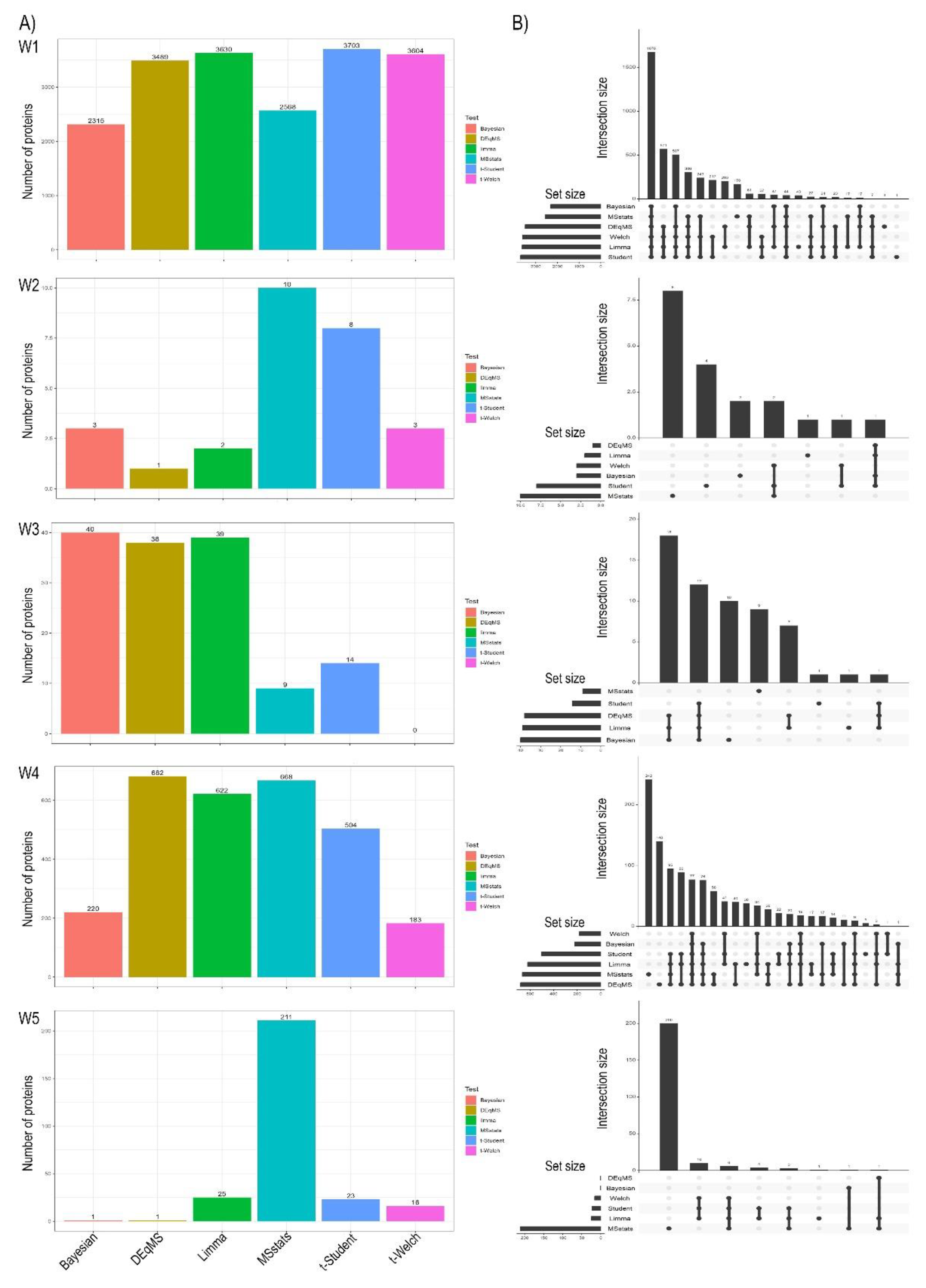
Figure 2.
Comparison of overlaps in the significant proteins in the different hypothesis tests after the biological relevance filter (fold change and Bayesian analysis). The overlap results of the identified proteins are presented for each of the frequentist methods (Student’s t, Welch’s t, Limma, DEqMS and MSstats) in Works 1, 2, 4 and 5 (A to D). Work 3 did not yield sufficiently significant results. B, proteins identified only after applying the biological relevance filter by the Bayesian method; FC, proteins identified only after applying the fold change filter; O, all proteins present after the hypothesis test.
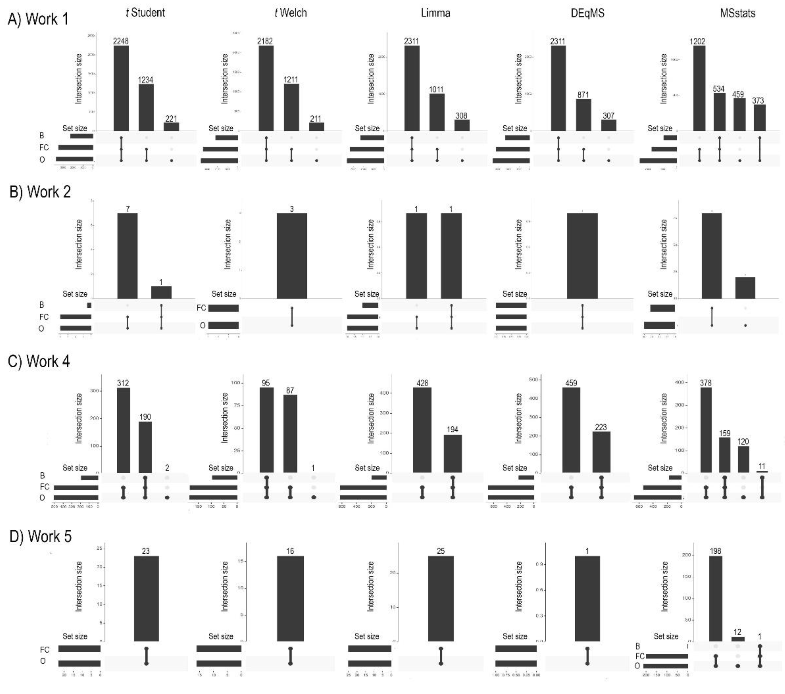
Figure 3.
Jaccard Similarity Distributions and Heatmaps of Functional Enrichment Terms. Panels A, B, and C illustrate Jaccard similarity distributions (top row, boxplots) and corresponding heatmaps (bottom row) of enriched functional terms across various comparison types for Work1 (upregulated proteins), Work4 (upregulated proteins), and Work4 (downregulated proteins), respectively. The boxplots show the distribution of arcsin(sqrt)-transformed Jaccard indices, categorized by comparison type: “Intra-HTM_FC_CBR” (concordance within Hypothesis Testing Methods with fixed Fold Change-based Criteria for Biological Relevance), “Intra-HTM_Bayes_CBR” (concordance within HTMs with fixed Bayesian-based CBR), “Intra-CBR_Fixed_HTM” (concordance within CBRs with fixed HTM), and “Inter-HTM_Inter-CBR” (concordance when both HTM and CBR vary). * p < 0.05, ** p < 0.01 (based on Kruskal-Wallis test and post-hoc Wilcoxon rank-sum tests as performed in the meta-analysis). Heatmaps represent pairwise Jaccard indices for terms across different methodological comparisons, with darker blue indicating higher similarity.
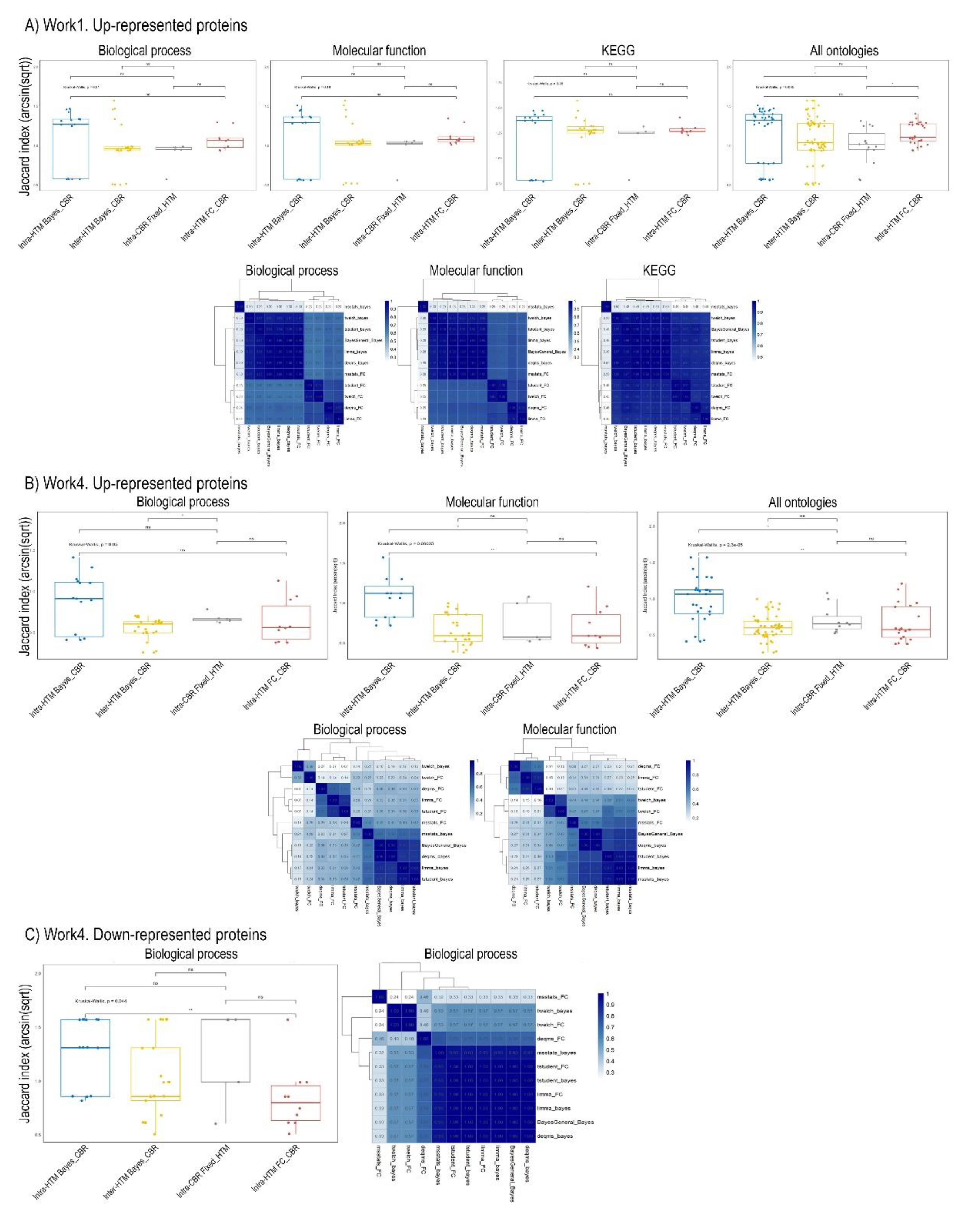
Figure 4.
Global distribution and comparison of Jaccard indices from meta-analysis. Panel A presents a histogram showing the distribution of the raw Jaccard Index values across all collected data. Panel B displays a histogram of the arcsin(sqrt)-transformed Jaccard Index values, illustrating how the transformation affects the data distribution. Panel C features boxplots representing the arcsin(sqrt)-transformed Jaccard Index values, categorized by four comparison types: “Intra-HTM_Bayes_CBR” (concordance among Hypothesis Testing Methods with Bayesian-based Criteria for Biological Relevance), “Inter-HTM_Inter-CBR” (concordance when both HTM and CBR vary), “Intra-CBR_Fixed_HTM” (concordance among CBRs with fixed HTM), and “Intra-HTM_FC_CBR” (concordance among HTMs with FC-based CBR). Each point represents a single Jaccard index calculation. The global Kruskal-Wallis p-value is displayed, indicating overall significant differences among the groups. Brackets with asterisks denote significance from post-hoc Wilcoxon rank-sum tests (ns: not significant, * p < 0.05, ** p < 0.01).
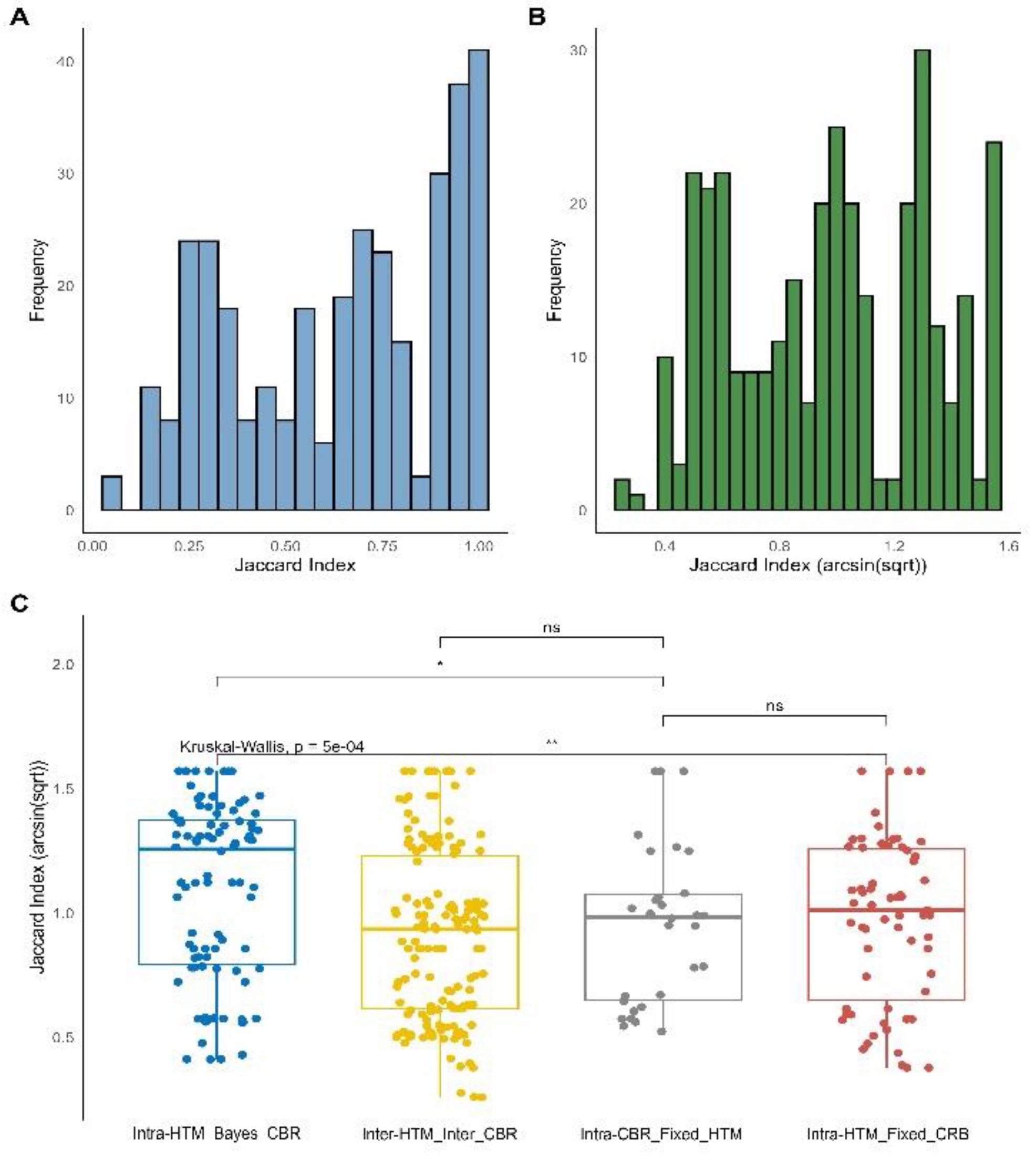
Figure 5.
Ontology-Specific and Sensitivity Analysis of Jaccard Similarity. Panel A displays boxplots of arcsin(sqrt)-transformed Jaccard Indices across the four comparison types, separated by specific ontologies: GO Biological Process, GO Molecular Function, and KEGG Pathways. Each subplot includes the Kruskal-Wallis p-value, and brackets with asterisks indicate significance from post-hoc Wilcoxon rank-sum tests (ns: not significant, * for p < 0.05, ** for p < 0.01). Panel B illustrates the sensitivity analysis by showing the Kruskal-Wallis p-values when each individual “Work” (dataset) is excluded from the meta-analysis. The dashed red line at p = 0.05 indicates the significance threshold. This panel highlights the influence of individual datasets on the overall statistical significance of the methodological comparisons.
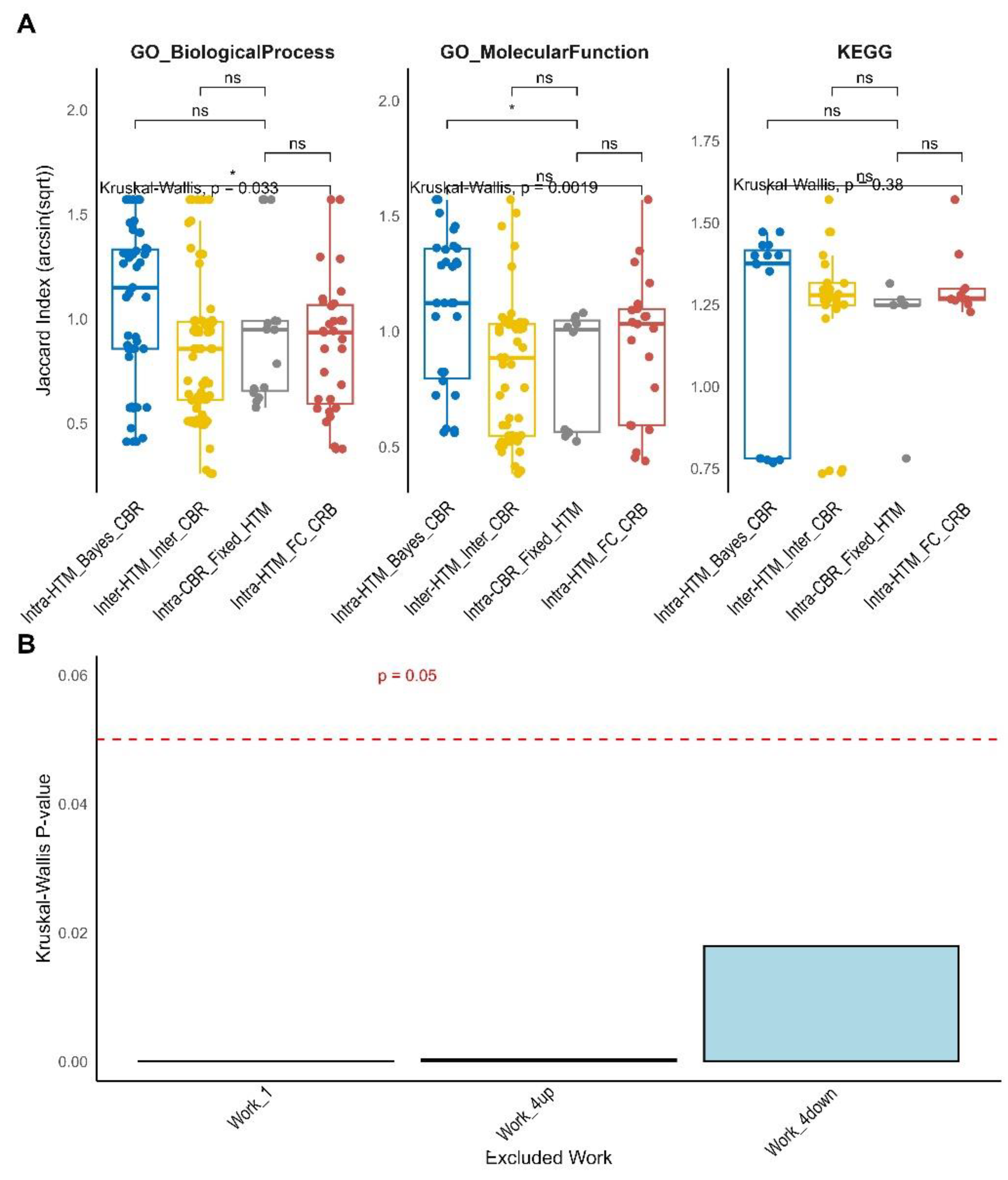

Table 1.
Recommended Statistical Tests for Quantitative Proteomics Differential Expression Analysis Based on Experimental Design.
Table 1.
Recommended Statistical Tests for Quantitative Proteomics Differential Expression Analysis Based on Experimental Design.
| Experimental Design | Most Commonly Used Test | More Appropriate Test |
|---|---|---|
| Simple Comparison (A vs. B) | Student’s t-test [23] | limma (moderated t-test) [25], DEqMS [26], Bayesian models [27] |
| Multiple Conditions | One-way ANOVA [28] | limma [25], DEqMS [26], Bayesian models [27] |
| Time Series Experiments | ANOVA / Linear Regression [28] | Linear mixed-effects models (MSstats) [28], limma [25], DEqMS [26], Bayesian [27] |
| Multifactorial (e.g., treatment × time) | Factorial ANOVA [28] | Mixed-effects models (MSstats) [28], limma [25], DEqMS [26], Bayesian [27] |
| Controlled Reference Mixtures | ANOVA / t-test [28] | limma [25], DEqMS [26], Bayesian [27] |
| Spectral Count Data | QSpec [29] | QSpec [29], hierarchical Bayesian count models [27] |
| Extended Time Series (>4 points) | Regression / Clustering [28] | Linear mixed-effects models (MSstats) [28], Bayesian time series [27] |
| Low Replication Designs | t-test / PLGEM-STN [23] | PLGEM-STN [23], limma [25], DEqMS [26], Bayesian [27] |
Table 2.
ProteinGroups variability. Cond1, condition 1 (Cold, Glu, NaCl, BNF and PM, respectively for each Work); Cond2, condition 2 (RT, Gly, No saline stress, no BNF, no PM, respectively for each Work). Levene p value shows the result of the Levene’s test (Equality of Variances): p-value > 0.05: There is no significant evidence to reject the null hypothesis that the variances between groups are equal; p-value <= 0.05: There is significant evidence to reject the null hypothesis of equality of variances (the variances between groups may be different).
| Work | Median CV (Cond1) (%) | Median CV (Cond2) (%) | SD del |Log2FC (Cond1 vs Cond2)| | Levene (p value) |
|---|---|---|---|---|
| 1 | 17.02 | 36.85 | 1.06 | 0 |
| 2 | 39.18 | 46.63 | 3.94 | 0.9313 |
| 3 | 17.16 | 12.92 | 2.73 | 0.1317 |
| 4 | 25.27 | 62.71 | 3.59 | 0.0117 |
| 5 | 74.69 | 62.2 | 3.9 | 0.001 |
Disclaimer/Publisher’s Note: The statements, opinions and data contained in all publications are solely those of the individual author(s) and contributor(s) and not of MDPI and/or the editor(s). MDPI and/or the editor(s) disclaim responsibility for any injury to people or property resulting from any ideas, methods, instructions or products referred to in the content. |
© 2025 by the authors. Licensee MDPI, Basel, Switzerland. This article is an open access article distributed under the terms and conditions of the Creative Commons Attribution (CC BY) license (http://creativecommons.org/licenses/by/4.0/).
Copyright: This open access article is published under a Creative Commons CC BY 4.0 license, which permit the free download, distribution, and reuse, provided that the author and preprint are cited in any reuse.


