
Submitted:
11 July 2025
Posted:
15 July 2025
You are already at the latest version
Abstract
Droplet-based microlens fabrication using UV-curable polymers demands precise meas-urement of three-dimensional geometries, especially for nonaxisymmetric shapes influ-enced by electric field deformation. In this work, we present a polar coordinate-based con-tour fitting method combined with Hermite interpolation to reconstruct 3D droplet geom-etries from two orthogonal shadowgraphy images. The image segmentation process inte-grates superpixel clustering with active contours to extract the droplet boundary, which is then approximated using a spline-based polar fitting approach. The two resulting con-tours are merged using a polar Hermite interpolation algorithm, enabling the reconstruc-tion of freeform droplet shapes. We validate the method against both synthetic CAD data and precision-machined reference objects, achieving volume deviations below 1% for ax-isymmetric shapes and approximately 3.5% for nonaxisymmetric cases. The influence of focus, calibration, and alignment errors is quantitatively assessed through Monte Carlo simulations and empirical tests. Finally, the method is applied to real electrically de-formed droplets, with volume deviations remaining within the experimental uncertainty range. This demonstrates the method’s robustness and suitability for metrology tasks in-volving complex droplet geometries.
Keywords:
3D reconstruction
; contact angles
; droplet deformation
; image processing
; optical simulations
; polar fitting
; polymer droplets
; image segmentation
; shape measurement
; volume estimation
; shadowgraphy
1. Introduction
Microlenses are small lenses with apertures between several micrometers and millimeters. They have emerged in recent years as important optical components in many technological areas, such as microlens arrays and optical fiber coupling, for example in biomedical applications. There are different methods for fabricating microlenses, such as hot embossing, lithography, inkjet printing, or more recently, two-photon polymerization [1,2,3]. Among these, the approaches using liquid-based photopolymerization offer a significant advantage due to the inherent energy minimization properties of the liquids, making it possible to achieve smooth optical surfaces with little or no post-processing [4,5,6]. However, the control of the shape of the liquid droplets is still an area of active research, particularly regarding the use of electric fields. The first experiments in this field were conducted by Taylor, who discovered that the application of a high electric field on a liquid deforms the liquid and leads to electrospraying [7]. This concept has since been used in many publications to deform liquid droplets, for example for adaptive optics [7] or for deformed and subsequently solidified aspherical lenses [8]. When the droplet is axisymmetric, the measurement of its contour is straightforward and can be achieved in several ways. An often used method is the Axisymmetric Drop Shape Analysis (ADSA), where the shape and the surface tension are related and the Laplacian equation of capillarity is used to iteratively calculate the droplet shape [9]. More recent approaches include Hou et al.’s use of two mutually perpendicular ellipses (TMPE) to approximate the shape of an axisymmetric droplet deformed by gravity, and similarly, Tran et al. used asymmetrical ellipses to describe the contour of droplets with large contact angles [10,11]. Wang and Yu used an ellipse to approximate sessile droplets on flat and spherical surfaces [13].
For real freeform geometries, however, the droplet is not axisymmetric. For such non-axisymmetric shapes, the above methods cannot be used. There has been significant development to describe the contour of non-axisymmetric sessile droplets. Timm et al. used hydrodynamic equations to describe droplets on an angled surface [12], while El Sherbini and Jacobi applied a two-circle fitting method to droplets on inclined surfaces [13]. Bateni et al. and Quetzeri-Santiago et al. used polynomials to determine only the contact angles of sessile droplets [14,15]. Andersen and Taboryski utilized a subpixel edge detection scheme developed by Trujillo-Pino et al. to characterize dynamic contact angles [16,17]. Stalder et al. developed a snake-based approach using b-splines and reflections of the droplet [18]. For non-axisymmetric inclined droplets, Rotenberg et al. described the shape using biquadratic spline functions [21]. All of these methods require extensive knowledge about the droplet, which limits their application to real freeform geometries. Furthermore, none of these methods provide a practical or validated way to reconstruct the full 3D geometry of electrically deformed, non-axisymmetric droplets using just two orthogonal views. This represents a critical methodological gap.
For optical components, a purely two-dimensional contour is not sufficient when the droplet is not axisymmetrical. In such cases, a three-dimensional description is required. The reconstruction of the 3D shape of sessile droplets presents additional challenges. The simplest approaches involve using the Pappus centroid theorem [22] or summed circular slices [23]. El Sherbini and Jacobi extended their two-circle method by integrating the contour over the circumference of the base [15], however, this approach fails for droplets with freeform geometries. Ríos-López et al. demonstrated a method to reconstruct the 3D geometry of a droplet by combining side and top images [19]. Brown et al. used the finite element method to describe the 3D shape of a non-axisymmetric droplet on an inclined surface where gravity plays a significant role [25]. Other mathematical techniques include the use of Bézier curves for meniscus shapes by Lewis and Matsuura [20], and the application of cubic splines to describe the axisymmetric shape of rotating droplets by Jakhar et al. [21].
Many of these reconstruction methods originate from inkjet printing. For instance, Nguyen et al. reconstructed non-axisymmetric flying droplets using the multiplicative algebraic reconstruction technique (MART) [28]. In the same field, an effective method for analyzing flying droplets involves slicing the droplet into pixel-height disks and calculating the cumulative volume, based on the assumption that flying droplets maintain circular cross-sections at each slice level [22,23,24]. This technique has also been adapted for calculating the volume of pendant drops [34]. While these methods are conceptually diverse, they share limitations: they are computationally intensive, require many viewpoints, or assume axisymmetry. None are designed for sessile, non-axisymmetric droplets imaged with only two cameras.
More recent advances in 3D reconstruction explore imaging and computational methods: Fu and Liu, as well as Masuk et al., applied the visual hull method with space carving, focusing primarily on bubble geometries [29,30].
The methods described offer a wide range of strategies for calculating both the two-dimensional contour geometry and the full three-dimensional shape and volume of droplets, whether sessile, flying, or pendant. However, these methodologies exhibit significant limitations when applied to electrically deformed, non-axisymmetric droplets, as examined in the present study. This research aims to address the identified gap. Furthermore, few studies address practical aspects such as image focus, segmentation robustness, or calibration stability, all factors that critically influence the accuracy of volume reconstruction but are often neglected.
2. Experimental Setup
The underlying aim of the experiments is to deform a UV-curable polymer droplet, which is then cured to preserve geometry and to manufacture microlenses. This experimental setup is designed to perform two primary functions. First, it must be able to generate and adjust a high-voltage electrical field. Second, the setup is required to observe and record the deformation data, including the voltage measurements. The setup is illustrated in Figure 1 (a). A high-voltage power supply (hivolt HAR42-4 with HA3B3-S) capable of delivering up to and noise of less than is employed. Voltage control and data acquisition are handled by a National Instruments USB-6001 card which has an accuracy of 26 mV and noise of . Two orthogonal shadowgraphy sets are used for imaging the experiment, placed 90 ° apart. In Figure 1 (b) a shadowgraphy image of an experiment is shown. Each set-up includes a grayscale camera (Matrix Vision MV 1013G-1111 with 1280 x 1024 resolution and 5.3 µm pixel size) paired with a zoom lens (Thorlabs MVL6X12Z). The lowest magnification setting of 1.4x provides a depth of field of 0.95 mm. This magnification is used for the conducted experiments. Illumination is provided by a white LED (Opto Engineering LTCLHP016-W LED) with a diffuser that suppresses diffraction artifacts at the edges. The diffuser is made from a Leica Surgipath Apex Adhesive Slide. Figure 1 (c) shows the complete optical setup. At the intersection of the X and Y optical axes, two motorized stages (Thorlabs PT1-Z825) are positioned to focus the droplet. The Z movement of the droplet is done using a manual stage because the Z movement is only needed to move the droplet into the cameras field of view. A set of three of the same motorized stages with a resolution of 0.05 µm resolution and repeatability under 1.5 µm is used to precisely move the anode along the X, Y, and Z axes. A tool-changing system (Schunk SHS) is employed for eased swapping of the anodes. An array of precision connectors (RM 2.54mm) serves as the anode, with a 6mm pin or an aluminum plate as the cathode. The anode configuration is shown in Figure 1 (d), where the shown anode connects to the positive pole and the cathode to the negative pole of the power supply.
The entire setup is housed within an electrically grounded security box, maintaining a constant temperature of 17° C with a precision of ±0.5°C. Temperature is monitored at seven positions inside the box (using 5 PT1000 Heraeus M102 sensors and 1 BME680 sensor) and at one external position (1 BME680 sensor).). The BME680 sensors also measure humidity and pressure. MATLAB R2024a is used to control the entire system.
To create ground-truth data of the droplets, the cameras need to be calibrated. The state-of-the-art method is Zhang’s method. That is why both cameras are calibrated individually using MATLAB's implementation of Zhang's method for camera calibration, using a distortion target (Thorlabs R1L3S3P positive grid) [25]. The object in the optical path is automatically focused using the motorized stages and the Tenengrad focus measure [17]. All images are undistorted using the camera parameters calculated from the calibration. The root means squared position reprojection error is 0.3 pixels which corresponds to about 3 µm in both cameras. All experiments are conducted using this setup.
3. Image Processing and 3D Geometry Reconstruction Workflow
The complete proposed method is shown in Figure 2. First images with both cameras are captured as seen in Figure 2 (a) and (b). Using image segmentation and our newly proposed Polar-Based Contour Approximation (PBCA) the droplet contour can be extracted from both cameras as shown in Figure 2 (c). Combining these contours in three-dimensional space and using a Hermite interpolation scheme, a 3D geometry can be reconstructed. In Figure 2 (d) the two contours in three-dimensional space are shown and in Figure 2 (e) the reconstructed geometry is shown.
The components of this process are discussed in more detail in the following sections.
3.1. Segmentation of Droplet Contours via Superpixels and Active Contours
The droplet contour is segmented using a combination of conventional algorithms using MATLAB. The whole process is shown in Figure 3. The image looks like a lens with two curved sides, but in reality, the bottom half is just the reflection of the top half. Before the process, the image intensity is adjusted using 'imadjust', which enhances the contrast. After that the input image shown in Figure 3 (a) is segmented into so-called superpixels using the Simple Linear Iterative Clustering (SLIC) algorithm, which clusters pixels into coherent regions seen in Figure 3 (b). This step makes the subsequent segmentation step more robust. The number of superpixels that suits this optical system, image size and application was empirically determined to be 6916 [26]. Subsequently a graph cut algorithm called Lazy Snapping is used on top of the superpixels as seen in Figure 3 (c). This is an easy and robust way to get an initial mask for the next step. For the Lazy Snapping algorithm to work, it is required to define pixels as foreground and background pixels. Initially the central pixel of the undistorted grayscale image is the foreground pixel. Because the droplet is not always in the center of the image, a method is needed to ensure that the initial pixel is inside the droplet. This is done by searching for a pixel close to the initial pixel that has a threshold intensity of 50, which in the images used here has proven as good empirical threshold. This is used to initialize the foreground region for segmentation, shown as a red point in Figure 3 (c).
is the foreground pixel, the violet lines at the left and to the right edge of the image are the background pixels. (a) Input image. (b) SLIC Superpixels. (c) Lazy snapping with superpixels. (d) Mask after active contour. (e) Roberts extracted pixels.
Background pixels are defined as the rows of pixels on the left and right edges of the image, as seen at the edges in Figure 3 in violet. The resulting mask is also seen in Figure 3 (c). Subsequently, an active contour algorithm based on the Chan-Vese method is applied with 50 iterations to refine the droplet boundary, as shown in Figure 3 (d). This method minimizes the energy along the contour, resulting in a binary mask that describes the shape of the drop. The segmented image is further refined by morphological closing using a 10 pixel disk, to smooth the edges, and finally use Roberts edge detector to extract the final contour points, represented as pixel coordinates [27]. These points are shown as a red dashed line in Figure 3 (e) and are used for a further detailed analysis of the shape of the droplet.
3.2. Polar-Based Contour Approximation (PBCA)
The Polar-Based Contour Approximation (PBCA) method introduced here describes a droplet's contour by fitting it in a polar coordinate system rather than the conventional cartesian system, akin to the representation of a signature in image processing. [28]. A droplet has, because of its energy minimizing nature, a smooth surface and is generally circular in nature. The presented approach takes that into account. Another challenge in representing a smooth droplet surface from pixelated data captured by a camera is the step-like distribution of the data. Particularly at the apex region of the droplet, the pixel representation is inadequate, because it is a horizontal line due to the discretization. Using our method, this straight line is transformed into a curved representation in polar coordinates, which makes approximating the points with a spline or polynomial more accurate. Figure 4 illustrates the entire methodology, and a detailed explanation is provided in the subsequent sections.
Converting the points to polar coordinates causes variations in their polar angles at the edges due to the tilt and their non-central positioning around zero. That can lead to significant jumps in the radial distance at and 0. This is why we limit the points in polar coordinates between and . For this the contour needs to be tilted and centered. The process begins by identifying the left and right contact points of the droplet along its contour. This identification occurs either by hand or algorithmically. The tilt angle β required to make the droplet leveled at these points is determined by
Using this angle, a rotation matrix is used to rotate the contour points. The rotated points are then shifted to center the contour around the origin with
and then the points are centered around zero in x direction, and the z coordinates are limited to values larger than zero using
with as aligned x and z points. Due to the discretization, the exact positions of the edge points are difficult to determine. The approach we use in PBCA is to extend the segmented contour with 10 pixels of the edge areas of the contour. This avoids approximation errors due to pixels at the contact points. This can be seen in Figure 4 (a), with the original contour in red with the mirrored extensions in green. Next, the aligned contour coordinates are transformed from Cartesian to polar coordinates , where represents the angular position and represents the radial distance from the center with
One challenge presented by the transformation is the uneven distribution of points across the angle , dependent upon the initial point distribution in cartesian coordinates. For a precise approximation, it is optimal when the points are uniformly distributed within the specified limits. To achieve this uniform distribution, the curve is pre-stretched prior to transformation, ensuring that the maximum height of the droplet is equivalent to half of the droplet's diameter. This ensures that the curve that is approximated, is always roughly the same shape, even when the contour is not axisymmetric. This also achieves an almost equidistant distribution of the points in polar coordinates. A polar plot of the unstretched in red and the stretched contour in blue is shown in Figure 4 (b). To have a continuous contour, the coordinates are sorted by sorting the angular coordinates in ascending order. An unwrapped plot of and is shown in Figure 4 (c). Next a b-spline is approximated on using MATLABs implementation of least-squares b-spline approximation [29]. The knot points for the spline interpolation are selected in a two-step process. First, the minimums and maximums of the curve are found. They are used as a knot with additional points between the ends. It was determined that for the droplets utilized in the present study, employing a total knot number of 30 and a spline degree of 9 is the optimal configuration for the geometries under investigation. For the final knots the MATLAB implementation of the “optimal” knot distribution is used [30,31,32]. This approximation smooths the contour while preserving its overall shape. Once the approximation process is complete, the fitted radial coordinates fit is transformed back into cartesian coordinates using the following equations
After transforming, the stretching is reversed. These fitted coordinates now provide a smooth approximation of the droplet's contour as seen in Figure 4 (d).
The PBCA method proves effective for the analysis of discretized irregular or complex geometries that exhibit smooth contours. The suitability of this is particularly notable in the characterization of droplet contours, as the approximated contour starts with an accurate representation of the contact point. This effectiveness was previously identified by Atefi et al., who employed the transformation from Cartesian to polar coordinates to estimate the contact angles of droplets [33]. Another inherent advantage is that PBCA does not suffer from the ambiguity that is present when a droplet has a contact angle over 90°, because in polar coordinates the angles are unique while in cartesian coordinate for one x value multiple values of y are necessary to describe a droplet of that shape.
3.3. D Geometry Reconstruction via Hermite Interpolation (PHDR)
The PBCA is used on the images of both cameras, which results in two slice representations of the droplet from two sides with an angle of 90°. The challenge presented is to reconstruct the 3D shape of the droplet using only these two slices. Each contour is represented in polar coordinates, and . Although both cameras are calibrated, there is still some small deviation between the maximal points of the droplet. To account for that, they must be scaled to avoid numerical errors. The scaling factor is calculated as a factor of the maximum heights with
A critical step in the reconstruction involves the calculation of the midpoints for each contour. This is necessary to align the two slices to each other and to obtain the points in each z-plane. This is done by numerical calculation of the midpoint on any given z-height. The midpoints are shown in Figure 5 (a) for the x-slice and in (b) for the y-slice. The contour lines are then combined and aligned at 90 ° to each other, corresponding to the orientation of the cameras. This is done using a three dimensinal rotation matrix.
For the reconstruction of each z-slice, two points from each x- and y-slice are needed at the same given z-height. The aligned slices and the resulting points and can be seen in in Figure 5 (c). The objective is to transform these points into a slice shape that closely approximates reality. The most straightforward method for interpolation would typically involve circular or elliptical approaches. However, we employed an interpolation algorithm known as polar coordinate Hermite-interpolation-based droplet reconstruction (PHDR), which was first introduced by Liu et al. and has been demonstrated to be superior to circular or elliptical methods [34]. It uses a modified cubic Hermite interpolation, which considers the inherent shape of the droplets. Because the projection direction is tangential, the derivative along this direction is zero, which simplifies the Hermite formulation. The input points are transformed into polar coordinates, resulting in four radii and angles per slice. The modified interpolation equation is
where and are the indices of the points in the z-plane and is the reconstructed curve using PHDR. The points and the reconstructed curves are shown in Figure 5 (d). This is repeated for each z-value, which leads to a reconstructed point cloud representation of the droplet, which can be seen in Figure 2 (e). The optimal balance between accuracy and computation time was achieved with arc-length sampling by using a sample size of 1000.
3.4. Numerical Volume Estimation from Reconstructed Contours
The volume calculation is performed analogous to Liu et al., employing numerical integration of the resulting contour by means of the Shoelace formula within cartesian coordinates for each slice to determine the areas . Subsequently, these areas are utilized to estimate the volume between two slices through summation and multiplication, as delineated by the following formula
with as reconstructed volume, as number of slices, as height between the area and . In conclusion, the combination of PBCA and PHDR provides a method for reconstructing 3D geometries from two shadowgraphy images.
4. Validation Experiments and Error Analysis
In this section, a series of experiments are conducted to show the effectiveness and limitations of the proposed contour approximation and the 3D reconstruction method. This is done in subsections; first, the polar PBCA interpolation method is compared to other standard methods of approximation with synthetic data. Then the 3D reconstruction is tested with known geometries, real and synthetic, to show the effectiveness of our combined method. Furthermore, Monte Carlo simulations are used to assess the stability of the process and the effects of focus and repeated measurements. In the end, experimental research is conducted using electrically deformed droplets, which serve as a benchmark by being weighed. Then, our method allows for the calculation of the volume based on the material's density, and this is compared to the weight measurement.
4.1. Evaluation of PBCA on Synthetic Geometries
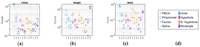
Since there are no valid approaches for the application to represent the droplet geometry of nonaxisymmetric droplets that are produced by electrical field deformation, PBCA is compared to common methods of approximating freeform shapes that are close to the real observed data. Here a polynomial least squares approximation of eighth degree, a Fourier least squares approximation of eighth degree, and a b-spline least squares approximation are used for comparison. The synthetic shapes, chosen to represent the droplet deformation observed in previous experiments, contain rounded edges, exhibit high and low contact angles, feature off-axis shapes, and have near-rectangular cross sections, reflecting the range of deformation observed. To evaluate the performance of the fit, we look at the important defining features of a non-axisymmetric droplet, such as the droplet diameter , the contact angles and as well as the apex position defined by and . These are shown in Figure 6 on a schematic droplet.
The contact angles are calculated using a linear regression of the initial ten pixels at the edges and using the slope to calculate the contact angles trigonometrically. The apex position is calculated by finding the maximum of the droplet contour, and the diameter is the difference between the first and last contour points. The geometrical shapes consist of circle segments, hyperbolas, slanted hyperbolas, and a sigmoidal function to account for rectangular shapes observed in multiple-anode arrangements. These shapes are chosen because they all occur in the deformation of droplets. The data used to evaluate the performance of PBCA is generated using the equations for the various shapes laid out in the next few paragraphs. The shapes are sized, so that they fit into the virtual image with an image width of and an image height , to be of the same size as the used cameras. To discretize the data, the values of x and y are rounded. For a circle, the equations are
with as circle coordinates, as circle radius and as the angle of the circle point. Circle segments are generated by defining the angle specific to the desired segment. For the hyperbola, the formula is
with and as hyperbola coordinates, as horizontal stretch factor and as vertical stretch factor. The slanted hyperbola has the same equation with and , but is tilted using a rotational matrix. The rotation is defined as . The rectangular form is generated using a function with sigmoidal properties. It is defined by two hyperbolic tangent functions combined with the formula
with and as rectangular coordinates, as distance of slope from zero an and as a parameter to control the slope. The used values for a, b, c, , and are shown in Table 1. The curves are then scaled so that the droplet base is half the image width and the maximum height is one fifth of the image height using
with and as scaled coordinates and and as unscaled coordinates.
This ensures similarity to the droplet contours observed in the deformation experiment. The drop image, after which the curve is modeled as well as the three curves are shown in Figure 7 (a) to (d).
To compare the measurement with the ground truth data, three metrics are used. For evaluating the overall fit over the whole contour, the root means square error (RMSE) between the approximated curve and the ground truth curve is calculated with the equation
with as root mean square error, n as number of points, G as ground truth data, and A as approximated data. To evaluate the performance over the non-axisymmetric metrics such as the contact angles and the diameter, which are in different units and magnitudes, the mean absolute percentage error (MAPE) is calculated using
with as the mean absolute percentage error. An alternative metric to compare the same is the mean normalized error (MNE).
with as the mean normalized error and R as value range, in this case for the angles and for the lengths which corresponds to the drop base diameter. The comparison results are shown in Figure 8 as boxplots. In Appendix A.1 all measurements are shown.
In the findings across all geometries, while PBCA may not consistently be the top performer, it demonstrates the greatest reliability. Notably, the results for MAPE and MNE indicate that PBCA exhibits less variability compared to other methods. As these two metrics directly measure errors in parameters specific to droplets, such as diameter, this underscores its suitability for addressing issues related to deforming droplets. Next, the 3D reconstruction is tested.
4.2. Accuracy of 3D Reconstruction Using CAD and Measured References
Initially, the approach is assessed using synthetic images that originate from 3D models generated through CAD software, specifically PTC CREO PARAMETRIC 10. For comparison with the reconstruction geometry, the models were converted to stereolithography (STL) files. To minimize the effect of sampling, the STLs are triangulated with the minimum possible step size of the triangulation mesh. These STL files are then imported into MATLAB, and the triangulation nodes are used as ground truth point cloud. The images that will be used for reconstruction are generated using the CREO render feature. Subsequently, PBCA is applied with PHDR to reconstruct the 3D geometry and calculate the volume. The used geometries are like the in Figure 7 used geometries circle, hyperbola, slanted hyperbola and rectangle. The configurations consist of a semisphere depicted in Figure 9 (a), an on-axis deformed droplet shown in Figure 9 (b) and an off-axis deformed droplet in Figure 9 (c).
To calculate the volume, the scaling factor per pixel is needed for each model, to convert the pixel values to SI units. The scaling factor is determined by counting the pixels of the base and is calculated using
with as scaling factor, as base measurement in pixel and as a base measurement in millimeters of the CAD model. For the three geometries, the reconstruction is carried out as previously said with a sampling of 1000. To align the point clouds, the STL point cloud and the reconstructed point cloud are registered using the ICP algorithm [35]. Subsequently the RMSE between the ground truth geometry and the reconstructed geometry is calculated as well as the volume of the reconstructed model and the absolute volume difference between the ground truth and the reconstructed model. The volume is here used as metric to evaluate how close the reconstructed and ground truth data are. These values as well as the scaling factors, base measurements, volumes and between the points of the ground truth STL and the reconstructed geometry are shown in Appendix A.2. The volume metrics and RMSE metrics are shown in Table 2. For the rectangular structure, our algorithm does not work. For the algorithm to work, there needs to be a single maximal point with no local minima. This is not the case for the rectangular structure, thus limiting our algorithm. For the other geometries the local Euclidean distance between the ground truth and the reconstructed geometries are shown in Figure 9 (d) to (f). What is evident in all three plots is the wavy distribution of the distance. This probably stems from spline interpolation in the polar coordinate system, as splines are oscillating around the knots. Overall, the best reconstruction is the one of the semisphere, with the maximum distance at around 3 microns. The on-axis deformation also has a small distance, the maximal distance being around 10 microns, but compared to the size of the whole object of 3 mm diameter, this is still quite small. The worst of the three is the geometry that is modeled on the off-axis deformation. There are two symmetric areas where the distance is around 50 microns. This is likely due to the way the reconstruction algorithm combines the two contours. The deviation is still not large compared to the whole structure of here 10 mm. In summary our approach works very well with axisymmetric geometries with a less than 3 microns and volume deviation of well under one percent. The non axisymmetric case is still good with a of just above 20 microns which is a tenfold increase compared to the axisymmetric case and a volume deviation of 3.5%.
In addition to the droplet-like shapes, a more extreme geometry is tested with the algorithm, which normally is not easy to represent with any other approximation that is not defined piecewise. It is a pyramid and a crooked pyramid. The methodology is the same as for the other CREO models. In Figure 10 (a) the x and y-view of the pyramid in CREO is shown, in Figure 10 (b) the crooked pyramid is shown. The Euclidean distance between the ground truth and the reconstructed models are shown in Figure 10 (c) and Figure 10 (d). As before, these geometries are represented rather well. A limitation that becomes obvious immediately is at the tip of the pyramids. The tip of the pyramid has no good representation, because of the continuity constraints of the spline-based polar fitting, which always leads to a smoothed corner and not a sharp corner. As with the other CREO models before, the wavy structure can be seen.
The distances are approximately 20 microns, which are relatively small when considered with the 3 mm size of the whole models. This result hints that this algorithm could also be used for other applications, such as tips, with the limitation that very sharp corners are not represented well.
In the subsequent evaluation, actual images depicting measured geometries are utilized. Three specifically precision-machined pins with a circular section on top and a coordinate measurement machine (CMM) ball are used. The pins approximate the shape that droplets will assume on a pin with no external force, characterized by axial symmetry. Utilizing a coordinate measuring machine (CMM), measurements were taken for three pins. Each pin features a base with a diameter of 5 mm. The radii of their circular sections are 2.56 mm, 3.63 mm, and 6.5 mm, respectively. The probing ball of the CMM has a diameter of 3 mm. These objects were put into the shadowgraphy setup, focused, and then images were taken with the X- and Y-cameras. These images can be seen in Figure 11 (a) to (d).
As with the synthetic CREO data, the PBCA is applied with PHDR to reconstruct the 3D geometries. But first the circular section must be isolated by manually finding the points where the pin and the circular section meet. This was done for all three pins. For the CMM ball, only half of the ball was used to reconstruct the geometry. This ensures that a comparable portion of the ball is used. Then the ICP algorithm is used to align the ground truth and the reconstruction and subsequently the RMSE between the ground truth geometry and the reconstructed geometry is calculated as well as the volume and the volume difference . Furthermore, the maximal Euclidean distance between the point clouds is calculated. The measurements of the ball and the pins are shown in Table 3. The full data is shown in Appendix A.3.
In Figure 11 (e) to (h) the local Euclidian distance is shown for each object. Like the reconstruction of the synthetic CREO data, the distance also has a wavy nature as seen especially in Figure 11 (e) and (f), stemming from the knots of the spline interpolation. For the two pins with a smaller radius and the CMM ball, the deviations are rather small with a maximum distance of 14 and 10 microns, as well as small RMSE of around 4 microns for the two pins and 2.48 microns for the CMM ball. The volume is also accurate with a deviation of less than 0.3% for the pins and the ball. The outlier here is pin 3 with a large radius of 6.5 mm. Analogous to a droplet balancing on a pin, this theoretical droplet would show very small contact angles. As illustrated in Figure 11 (g) the plot showing the distance of pin 3, a significant divergence appears exactly at the junction between the pin and the curved segment, which is marked with red arrows. This finding indicates a constraint in our algorithm's ability to precisely handle small contact angles.
4.3. Focus Sensitivity and Uncertainty Analysis
In the calculations, the focus seemed to have an impact on how accurate the shape and volume are calculated. To test the extent, we did two experiments to test the influence of volume, general RMSE deviation, and focus. First, we randomly moved the CMM ball along the optical axes of both cameras and took an image at each step. Second, we used our autofocus to first focus both axes and then take an image of the CMM ball and repeat this step multiple times. The first experiment quantifies how image sharpness impacts volume estimation and the second tests whether autofocus maintains high focus and reduces variability. Then we use these images in both cases to calculate the Tenengrad focus measure to evaluate the focus in the image and then we use our algorithms to calculate the 3D shape and the volume. We did this with both cameras, because although they have the same components, they have a slight difference in image quality. The magnification and sharpness are slightly different, despite being the exact same components. The CMM ball in the first experiment in the setup with the movement direction is shown in Figure 12 (a). In Figure 12 (b) and Figure 12 (c) in blue the calculated volumes for the moving CMM ball are shown and the red line is the Tenengrad measure. Camera X records the movement on the Y-axis, and camera Y records the movement on the X-axis. Additionally, the actual volume is indicated by a dashed horizontal line, and the maximum sharpness is indicated by a full vertical line. The same is depicted in Figure 12 (c) for movement on the Y-axis. The graphs clearly demonstrate that as the image becomes more focused, the estimated volume approaches the true volume, indicating that our method is responsive to changes in focus.
To evaluate the relationship between image sharpness and reconstruction accuracy, we computed the correlation coefficient between the Tenengrad focus measure and the RMSE of the reconstructed shape. The Pearson correlation coefficient [36] is calculated using
with as correlation coefficient, as covariance of and and and as variance of and respectively. The correlation coefficient is computed by comparing the RMSE with the Tenengrad measure, illustrating how geometric deviation correlates with image sharpness. Specifically, for motion along the X-axis, a negative correlation of -0.63 is observed, while for the Y-axis, the correlation is more pronounced at -0.85. These values indicate a substantial reliance on geometric deviation relative to the image's focus. As seen in Figure 12 (b) and (c) the least deviation of the volume is where the image has the highest focus. This indicates not only that the volume is more correct with a more focused image, but also that the overall geometric shape is closer to the real shape with a better focus.
The thermal properties of the cameras were also examined in this experiment, as the cameras experience an increase in temperature over time despite the temperature-controlled setup. To understand the influence of the camera temperature, we tracked the camera temperature using the built-in temperature sensor of the cameras. The X-camera exhibited a mean temperature of 44.49°C, with a standard deviation of 0.16°C and a variance of . In contrast, the Y-camera recorded a mean temperature of 40.61°C, accompanied by a standard deviation of 0.30°C and a variance of . These findings indicate a discrepancy in the thermal characteristics of the two cameras. The root cause of this variation remains unidentified; nonetheless, it is likely due to differences in the cameras and their placement inside the temperature-controlled box, which exhibits slight temperature fluctuations. The correlation coefficient between temperature and the Tenengrad measure is 0.2 for the X-camera and 0.16 for the Y-camera, signifying a weak correlation across the temperature spectrum, suggesting that small absolute temperature fluctuations have a negligible effect on image sharpness and reconstruction quality..
We carried out the second experiment, which was mentioned earlier, to evaluate the effectiveness of our autofocus mechanism by focusing on the CMM ball through both cameras. The real volume of the ball is as before . In this experiment the mean volume is with a standard deviation of which gives a 95% coverage interval of . Additionally, the RMSE of the STL data and the reconstructed volume were calculated for each reconstruction, resulting in a mean RMSE of 2.7 µm with a standard deviation of 0.8 µm, suggesting limited sensitivity in the shape reconstruction. Lastly, the correlation coefficients between the volume and the Tenengrad measure of both cameras were calculated to see if there is any correlation left with the autofocus. The correlation coefficients are for the X camera -0.06 and for the Y camera 0.03 indicating that the autofocus compensates for focus-related variability.
In calculating the 3D volume, we presuppose a 90° angle between the two cameras, yet our setup does not allow for precise measurement of minor deviations. Additionally, there is an imprecision in determining the contact points, which can be selected either manually or through an algorithm, specifically at the intersection of the pin and the circular section. To assess the uncertainties arising from both the camera angle and the determination of contact points, we performed a Monte Carlo simulation integrating images captured from pin 1, which possesses a radius of 2.56 mm. The contact points and angles were varied and subsequently the 3D shape was reconstructed, the volume was calculated, and the RMSE between the true STL shape and the reconstructed shape was calculated after aligning using the ICP algorithm. We assumed the true location to differ from the contact points found by a normally distributed random error with a standard deviation of 2 pixels. Angle noise is also assumed to be normally distributed, with a standard deviation of 5 °. We performed 10000 simulations. In Figure 13 (a) the pixel noise is shown for the left and right contact points for both cameras, and in Figure 13 (b) the camera angle over all simulations are shown. In Figure 13 (c) the histogram of the simulated volumes is shown, confirming that the normal distributed input noise leads to a normal distributed volume. In (d) the boxplot of the simulated volumes is shown.
The mean of the volume is with a standard deviation of . The 95% coverage interval is , the real volume of the circular shape of the pin is which lies well within the coverage interval, which indicates good agreement between reconstruction and ground truth data. The coverage interval is calculated here using the standard deviation, because the simulation is based on one measurement. The standard error of the mean is which indicates that the average of the monte Carlo simulations is stable numerically. The RMSE between STL and reconstruction was also calculated each time, resulting in a mean RMSE of 49 µm with a standard deviation of 0.7 µm. These small RMSE values confirm that the reconstructed geometry matches the ground-truth STL closely even with the added noise.
4.4. Real World Application: Electrically Deformed Droplet Volumetry
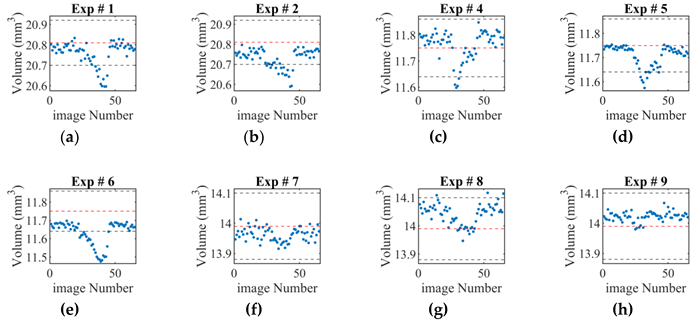
As final experiment, a real deformation experiment was conducted to test the algorithm in real world conditions with a droplet. For that we use the full setup that is described in 2. Measuring the true shape of a deformed liquid droplet directly is challenging, so we employed an alternative method to indirectly determine the accuracy of our method. To evaluate accuracy without measuring the real shape of the droplets, a comparing experiment was conducted. A droplet of known density was weighed, put into the setup, and recorded while it was deformed. The previous sections showed that the reconstruction of the shape and the volume is accurate using known axisymmetric shapes, specifically a spherical cap. The initial droplet shape is a spherical cap, which has an accurate shape and volume reconstruction. In this experiment, the idea is to show how much the volume is changing while deforming, which can give an indication how good the shape of the reconstruction is. Oleic acid is chosen as the material because of its nonevaporating and non-hygroscopic properties. The materials density was first measured using a Schmidt & Haensch EDM 4000+ density meter with an accuracy of . At the experiment the temperature of the density is . A 6 mm pin is placed inside a GRAM FV-120 analytical balance with an accuracy of 0.1 mg. These accuracies lead to an uncertainty of in the applied volume range. Afterward, a specified volume of the material is dispensed on top. The droplet is subsequently weighed and then put into the experimental setup, where it is subjected to an electric field with nonaxisymmetric deformation. The time between dispensing the oleic acid and the start of deformation is less than 5 minutes. The experiment begins with a one-second interval during which no voltage is applied, followed by a one-second interval of voltage application, and concludes with another one-second interval without applied voltage. The droplet on top of the pin in the balance is shown in Figure 14 (a). The anode that was used for this experiment is an elongated anode as seen in Figure 14 (b), as cathode the pin itself was used. This process was carried out with three volumes and different anode positions. In Figure 14 (c) and (d) the camera images of the X- and Y-cameras is shown.
Using this process of oleic acid droplet application, weighting and deformation, nine experiments were conducted. Of the nine experiments, the first three droplets had a weight of and a respective volume of , experiment four to six had a weight of and a respective volume of and experiments seven to nine had a weight of and a respective volume of . In Figure 15 an exemplary plot for all experiments of the resulting reconstructed volumes is shown over the course of experiment 5. The experiments 1 to 9 are shown in Appendix B.1. The image number here is the number of images that were taken since the start of the experiment. The third experiment is empty of data and thus not shown, because during the experiment, the droplet was obscured by the anode, which eliminates the application of our algorithm. If our algorithm would reconstruct the shape perfectly, then the volume would be constant. However, analysis of the synthetic data generated using a nonaxially deformed CREO model indicates that a minor error within the low percentage range is anticipated. If we look at the volume progression during the experiment, a few things can be derived. Initially, the volume, when there is no electric-induced deformation, matches the calculated volume within the experimental measurement uncertainty, indicating accurate reconstruction under these conditions. However, as the droplet undergoes deformation, the volume decreases, which hints at an increasing error in the reconstruction. The amount of decreasing is dependent on the experiment setup, although no systematics could be derived. The only systematic is, that the droplet volume reduces, hinting to an area that is not seen in the two shadowgraphy images. But when looking at the percentage error of the volume, that ranges between 0 and 3%. Although the maximum observed volumetric change was 3%, this remains within a realistic error range for non-ideal imaging setups.
This still provides good accuracy for the reconstruction of two images.
5. Conclusions
In this work, we presented a polar coordinate-based contour approximation (PBCA) with a Hermite interpolation strategy (PHDR) for approximating the contour and reconstructing various shapes focusing on nonaxisymmetric droplets under electric field deformation. Utilizing two shadowgraphy images, the proposed framework effectively circumvents conventional assumptions regarding droplet symmetry, thus providing reliable 3D shape and volume estimations. Numerical validations against synthetic CAD models and real references confirm that our approach maintains accuracy with volume deviations typically under 3%, while still being straightforward to implement.
The study further underscores the importance of proper focus and camera calibration in minimizing measurement error; as demonstrated, slight misalignment or defocus can notably shift volume and shape reconstructions. We observed a strong correlation between the image sharpness and the reconstruction accuracy but could limit this influence by autofocusing.
However, certain limitations remain. First, extremely sharp or rectangular cross sections like corners of pyramids are not captured correctly, suggesting that pure polar-based fits may need extensions for highly angular geometries. Second, heavy obstructions in one camera view can degrade the reconstruction if large portions of the droplet boundary are unseen. Furthermore, shapes where there is no maximal point like a rectangle, are also not reconstructable with this approach. Added noise to the camera angle and the contact points showed small but not significant deviations, showing the robustness of the method. Shape deviations also restrict this type of reconstruction to illumination optics only, because for other applications the deviations and especially the waviness is not acceptable.
Future work could incorporate multiview setups or advanced interpolation methods that better handle multipeak droplet surfaces. In practice, combining the polar-based method with real-time focus monitoring would further enhance reliability, especially in dynamic or industrial environments where droplets may shift or vibrate. With these refinements, the method promises to become an even more powerful tool for diverse metrology tasks, including adaptive optics, specialized lens fabrication, and broader microfluidic applications requiring detailed droplet shape measurements.
Author Contributions
Conceptualization MD, AH; Data curation MD; Formal analysis MD, AH; Funding acquisition AH; Investigation MD; Methodology MD, AH, CN; Project administration MD, AH; Resources MD, AH, CN; Software MD; Supervision AH, CN; Validation MD, AH, CN; Visualization MD; Writing - original draft MD; Writing - review & editing MD, AH, CN
Funding
This research was funded by the Deutsche Forschungsgemeinschaft (DFG) grant number HE 3533/10-1.
Data Availability Statement
The data presented in this study is available on request from the corresponding author.
Acknowledgments
The Author thanks Sascha Wallentowitz for helping to come up with the idea of the polar approximation as well as Felix Zeller and Lutz Autschbach of Carl Zeiss Jena for manufacturing the precision machined pins.
Conflicts of Interest
The authors declare no conflicts of interest.
Abbreviations
The following abbreviations are used in this manuscript:
| PBCA | Polar-Based Contour Approximation |
| PHDR | Polar-coordinate Hermite-interpolation-based Droplet Reconstruction |
| 3D | Three-Dimensional |
| CAD | Computer-Aided Design |
| CMM | Coordinate Measuring Machine |
| ICP | Iterative Closest Point |
| LED | Light Emitting Diode |
| RMSE | Root Mean Square Error |
| MAPE | Mean Absolute Percentage Error |
| MNE | Mean Normalized Error |
| STL | Stereolithography (file format) |
| DOF | Depth of Field |
| SLIC | Simple Linear Iterative Clustering |
| MDPI | Multidisciplinary Digital Publishing Institute |
| µm | Micrometer |
| °C | Degrees Celsius |
| µm/px | Micrometers per Pixel |
| px | Pixel |
| Reconstructed Droplet Volume | |
| ΔV | Volume Deviation |
| ROI | Region of Interest |
Appendix A
Appendix A.1
The color corresponds to the shape, blue is the circle, red is the hyperbola, yellow is the slanted hyperbola, and purple is the rectangle. The number corresponds to the extension of the shape as described.
Appendix A.2
All Values for the CREO data
| Semisphere | On axis | Off axis | |
| 1040 | 1070 | ||
| 906 | 1040 | 1138 | |
| 3 (X & Y) | 9 (X & Y) | 9.64 (X) 10.26 (Y) | |
| 3.31 | 8.65 | 9.01 | |
| 3.31 | 8.65 | 9.02 | |
| 7.069 | 61.499 | 99.893 | |
| 7.084 | 61.494 | 96.393 | |
| 0.015 | 0.005 | 3.5 | |
| 0.212 | 0.008 | 3.631 | |
| 0.0011 | 0.0028 | 0.0224 | |
| 0.33 | 0.324 | 2.486 | |
| Max distance (mm) | 0.003 | 0.010 | 0.056 |
| Max distance (px) | 0.906 | 1.156 | 6.215 |
Appendix A.3
All Data for the precision pins and the CMM ball
| Pin 1 | Pin 2 | Pin 3 | Cmm | |
| 2.56 | 3.63 | 6.49 | 1.5 | |
| 4.86 | 4.87 | 4.90 | 1.5 | |
| 19.21 | 9.21 | 4.59 | 7.07 | |
| 19.19 | 9.21 | 4.60 | 7.02 | |
| 0.02 | 0 | 0.01 | 0.05 | |
| 0.1 | 0 | 0.22 | 0.7 | |
| 4.28 | 4.17 | 11.15 | 2.48 | |
| Max Distance (µm) | 14.36 | 14.47 | 292.05 | 9.76 |
Appendix B
Appendix B.1
References
- Yuan, W.; Li, L.-H.; Lee, W.-B.; Chan, C.-Y. Fabrication of Microlens Array and Its Application: A Review. Chinese Journal of Mechanical Engineering 2018, 31, 16. [Google Scholar] [CrossRef]
- Cai, S.; Sun, Y.; Chu, H.; Yang, W.; Yu, H.; Liu, L. Microlenses Arrays: Fabrication, Materials, and Applications. [CrossRef]
- Marini, M.; Nardini, A.; Vázquez, R.M.; Conci, C.; Bouzin, M.; Collini, M.; Osellame, R.; Cerullo, G.; Kariman, B.S.; Farsari, M.; et al. Microlenses Fabricated by Two-Photon Laser Polymerization for Cell Imaging with Non-Linear Excitation Microscopy. [CrossRef]
- Frumkin, V.; Bercovici, M. Fluidic Shaping of Optical Components. Flow 2021, 1, E2. [Google Scholar] [CrossRef]
- Elgarisi, M.; Frumkin, V.; Luria, O.; Bercovici, M. Fabrication of Freeform Optical Components by Fluidic Shaping. Optica, OPTICA 2021, 8, 1501–1506. [Google Scholar] [CrossRef]
- Xu, C.; Guan, X.; Abbasi, S.A.; Xia, N.; Ngai, T.; Zhang, L.; Ho, H.-P.; Ng, S.H.C.; Yuan, W. Liquid-Shaped Microlens for Scalable Production of Ultrahigh-Resolution Optical Coherence Tomography Microendoscope. Commun Eng 2024, 3, 1–12. [Google Scholar] [CrossRef]
- Lima, N.C.; Mishra, K.; Mugele, F. Aberration Control in Adaptive Optics: A Numerical Study of Arbitrarily Deformable Liquid Lenses. Opt. Express, OE 2017, 25, 6700–6711. [Google Scholar] [CrossRef] [PubMed]
- Zhan, Z.; Wang, K. Fabrication of Aspherical Liquid Lens Controlled by Electrostatic Force. In Proceedings of the 3rd International Symposium on Advanced Optical Manufacturing and Testing Technologies: Advanced Optical Manufacturing Technologies; SPIE, November 14 2007; Vol. 6722; pp. 1038–1044. [Google Scholar]
- Saad, S.M.I.; Neumann, A.W. Axisymmetric Drop Shape Analysis (ADSA): An Outline. Advances in Colloid and Interface Science 2016, 238, 62–87. [Google Scholar] [CrossRef] [PubMed]
- Hou, B.; Wu, C.; Liu, H.; Sun, R.; Li, X.; Liu, C.; Wu, J.; Chen, M. Shape Approximation of Sessile Droplet by the Equivalence between Vertical Capillary Force and Hydrostatic Pressure. Colloids and Surfaces A: Physicochemical and Engineering Aspects 2023, 656, 130203. [Google Scholar] [CrossRef]
- Tran, D.T.; Nguyen, N.-K.; Singha, P.; Nguyen, N.-T.; Ooi, C.H. Modelling Sessile Droplet Profile Using Asymmetrical Ellipses. Processes 2021, 9, 2081. [Google Scholar] [CrossRef]
- Timm, M.L.; Dehdashti, E.; Jarrahi Darban, A.; Masoud, H. Evaporation of a Sessile Droplet on a Slope. Sci Rep 2019, 9, 19803. [Google Scholar] [CrossRef] [PubMed]
- ElSherbini, A.I.; Jacobi, A.M. Liquid Drops on Vertical and Inclined Surfaces: II. A Method for Approximating Drop Shapes. Journal of Colloid and Interface Science 2004, 273, 566–575. [Google Scholar] [CrossRef] [PubMed]
- Bateni, A.; Susnar, S.S.; Amirfazli, A.; Neumann, A.W. A High-Accuracy Polynomial Fitting Approach to Determine Contact Angles. Colloids and Surfaces A: Physicochemical and Engineering Aspects 2003, 219, 215–231. [Google Scholar] [CrossRef]
- Quetzeri-Santiago, M.A.; Castrejón-Pita, J.R.; Castrejón-Pita, A.A. On the Analysis of the Contact Angle for Impacting Droplets Using a Polynomial Fitting Approach. Exp Fluids 2020, 61, 143. [Google Scholar] [CrossRef]
- Andersen, N.K.; Taboryski, R. Drop Shape Analysis for Determination of Dynamic Contact Angles by Double Sided Elliptical Fitting Method. Meas. Sci. Technol. 2017, 28, 047003. [Google Scholar] [CrossRef]
- Trujillo-Pino, A.; Krissian, K.; Alemán-Flores, M.; Santana-Cedrés, D. Accurate Subpixel Edge Location Based on Partial Area Effect. Image and Vision Computing 2013, 31, 72–90. [Google Scholar] [CrossRef]
- Stalder, A.F.; Kulik, G.; Sage, D.; Barbieri, L.; Hoffmann, P. A Snake-Based Approach to Accurate Determination of Both Contact Points and Contact Angles. Colloids and Surfaces A: Physicochemical and Engineering Aspects 2006, 286, 92–103. [Google Scholar] [CrossRef]
- Ríos-López, I.; Karamaoynas, P.; Zabulis, X.; Kostoglou, M.; Karapantsios, T.D. Image Analysis of Axisymmetric Droplets in Wetting Experiments: A New Tool for the Study of 3D Droplet Geometry and Droplet Shape Reconstruction. Colloids and Surfaces A: Physicochemical and Engineering Aspects 2018, 553, 660–671. [Google Scholar] [CrossRef]
- Lewis, K.; Matsuura, T. Bézier Curve Method to Compute Various Meniscus Shapes. ACS Omega 2023, 8, 15371–15383. [Google Scholar] [CrossRef] [PubMed]
- Jakhar, K.; Chattopadhyay, A.; Thakur, A.; Raj, R. Spline Based Shape Prediction and Analysis of Uniformly Rotating Sessile and Pendant Droplets. Langmuir 2017, 33, 5603–5612. [Google Scholar] [CrossRef] [PubMed]
- Kim, S.; Choi, J.H.; Sohn, D.K.; Ko, H.S. The Effect of Ink Supply Pressure on Piezoelectric Inkjet. Micromachines 2022, 13, 615. [Google Scholar] [CrossRef] [PubMed]
- Hutchings, I.; Martin, G.; Hoath, S.; Martin, G.; Hoath, S. High Speed Imaging and Analysis of Jet and Drop Formation. Journal of Imaging Science and Technology 2007, 51, 438–444. [Google Scholar] [CrossRef]
- Thurow, K.; Krüger, T.; Stoll, N. An Optical Approach for the Determination of Droplet Volumes in Nanodispensing. Journal of Analytical Methods in Chemistry 2009, 2009, e198732. [Google Scholar] [CrossRef] [PubMed]
- Zhang, Z. A Flexible New Technique for Camera Calibration. IEEE Transactions on Pattern Analysis and Machine Intelligence 2000, 22, 1330–1334. [Google Scholar] [CrossRef]
- Achanta, R.; Shaji, A.; Smith, K.; Lucchi, A.; Fua, P.; Süsstrunk, S. SLIC Superpixels Compared to State-of-the-Art Superpixel Methods. IEEE Trans Pattern Anal Mach Intell 2012, 34, 2274–2282. [Google Scholar] [CrossRef] [PubMed]
- Roberts, L.G. Machine Perception of Three-Dimensional Solids. Thesis, Massachusetts Institute of Technology, 1963.
- Gonzalez, R.; Woods, R. Digital Image Processing Available online:. Available online: https://elibrary.pearson.de/book/99.150005/9781292223070 (accessed on 28 October 2024).
- Unser, M. Splines: A Perfect Fit for Signal and Image Processing. IEEE Signal Processing Magazine 1999, 16, 22–38. [Google Scholar] [CrossRef]
- Micchelli, C.A.; Rivlin, T.J.; Winograd, S. The Optimal Recovery of Smooth Functions. Numer. Math. 1976, 26, 191–200. [Google Scholar] [CrossRef]
- de Boor, C. Computational Aspects of Optimal Recovery. In Optimal Estimation in Approximation Theory; Micchelli, C.A., Rivlin, T.J., Eds.; Springer US: Boston, MA, 1977; ISBN 978-1-4684-2388-4. [Google Scholar]
- Gaffney, P.W.; Powell, M.J.D. Optimal Interpolation. In Proceedings of the Numerical Analysis; Watson, G.A., Ed.; Springer: Berlin, Heidelberg, 1976; pp. 90–99. [Google Scholar]
- A Robust Polynomial Fitting Approach for Contact Angle Measurements | Langmuir Available online:. Available online: https://pubs.acs.org/doi/10.1021/la4002972 (accessed on 28 October 2024).
- Liu, Q.; Chen, J.; Yang, H.; Yin, Z. Accurate Stereo-Vision-Based Flying Droplet Volume Measurement Method. IEEE Transactions on Instrumentation and Measurement 2022, 71, 1–16. [Google Scholar] [CrossRef]
- Pcregistericp Available online:. Available online: https://de.mathworks.com/help/vision/ref/pcregistericp.html (accessed on 5 March 2025).
- Krystek, M. Berechnung der Messunsicherheit: Grundlagen und Anleitung für die praktische Anwendung; Beuth Praxis Messwesen; 1. Aufl.; Beuth: Berlin Wien Zürich, 2012; ISBN 978-3-410-20932-4. [Google Scholar]
Figure 1.
Overview of Setup. (a) Sideview of setup. (b) Shadowgraphy image of an experiment. (c) Top view of the camera systems and the orientation. (d) Precision connector anode.
Figure 1.
Overview of Setup. (a) Sideview of setup. (b) Shadowgraphy image of an experiment. (c) Top view of the camera systems and the orientation. (d) Precision connector anode.
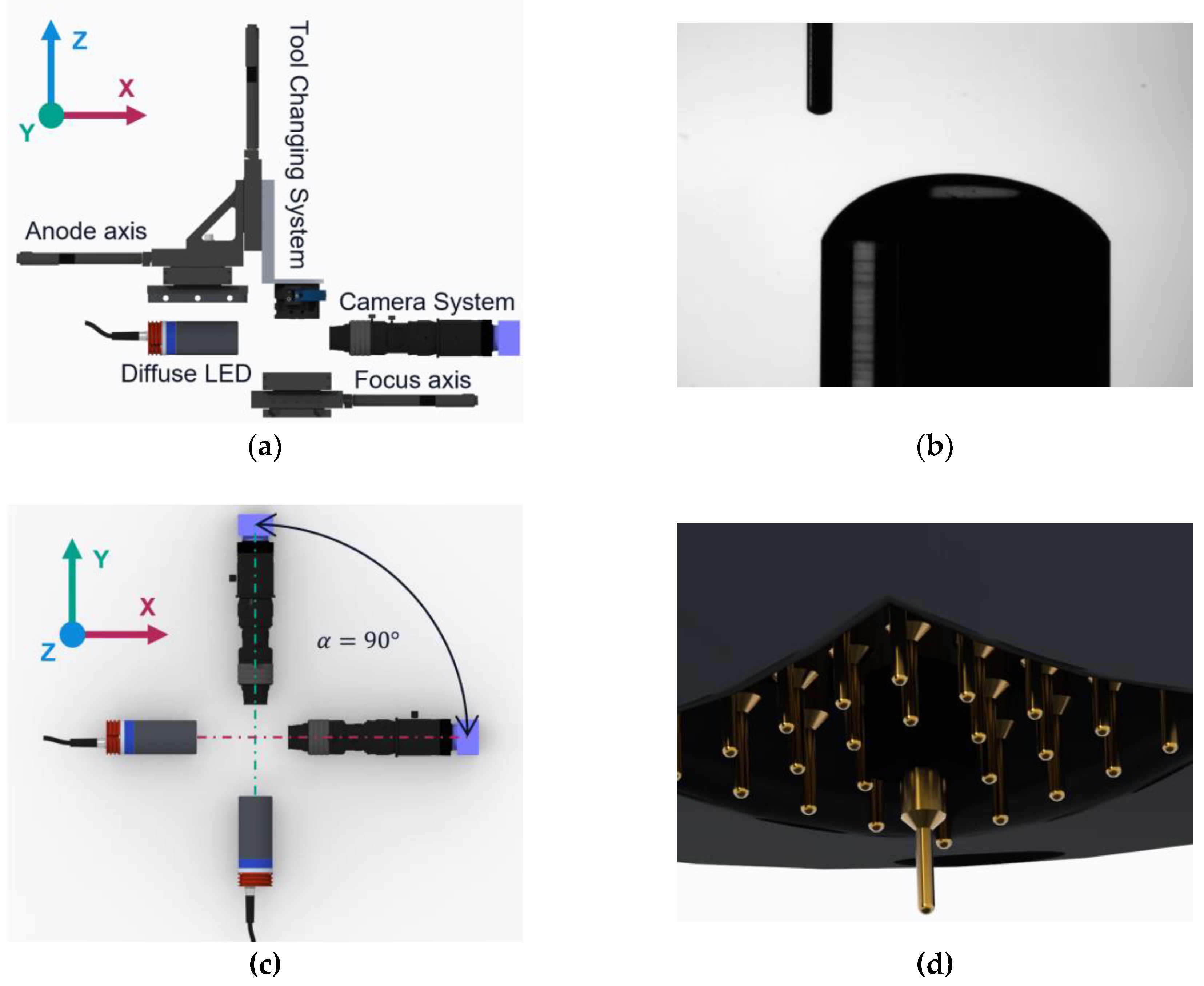
Figure 2.
Reconstruction process (a) Image acquisition. (b) Captured image. (c) Contour extracted fitted using PBCA. (d) Combined contours. (e) Reconstructed droplet geometry.
Figure 2.
Reconstruction process (a) Image acquisition. (b) Captured image. (c) Contour extracted fitted using PBCA. (d) Combined contours. (e) Reconstructed droplet geometry.
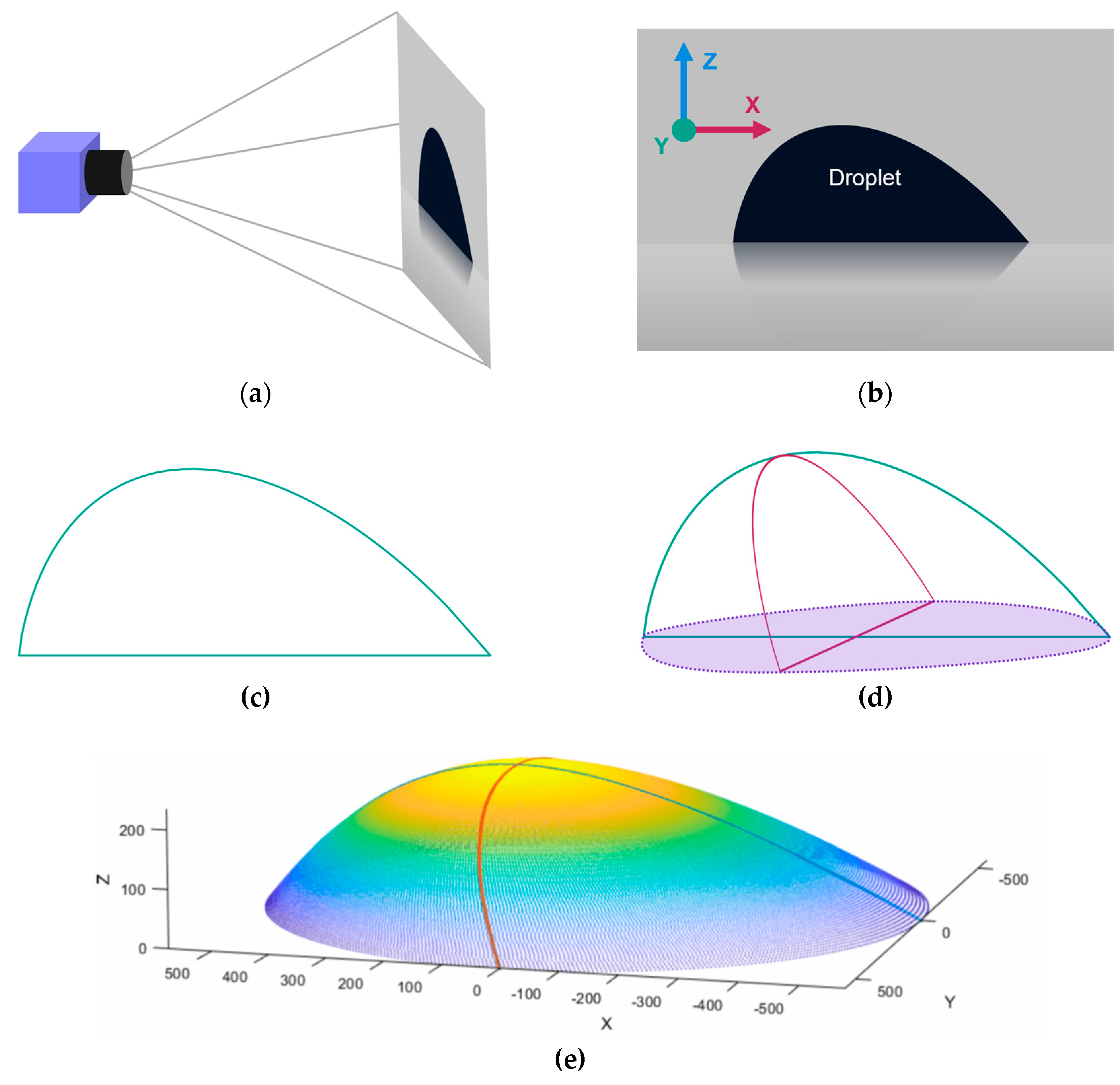
Figure 3.
Sequence of the image segmentation. The red point with
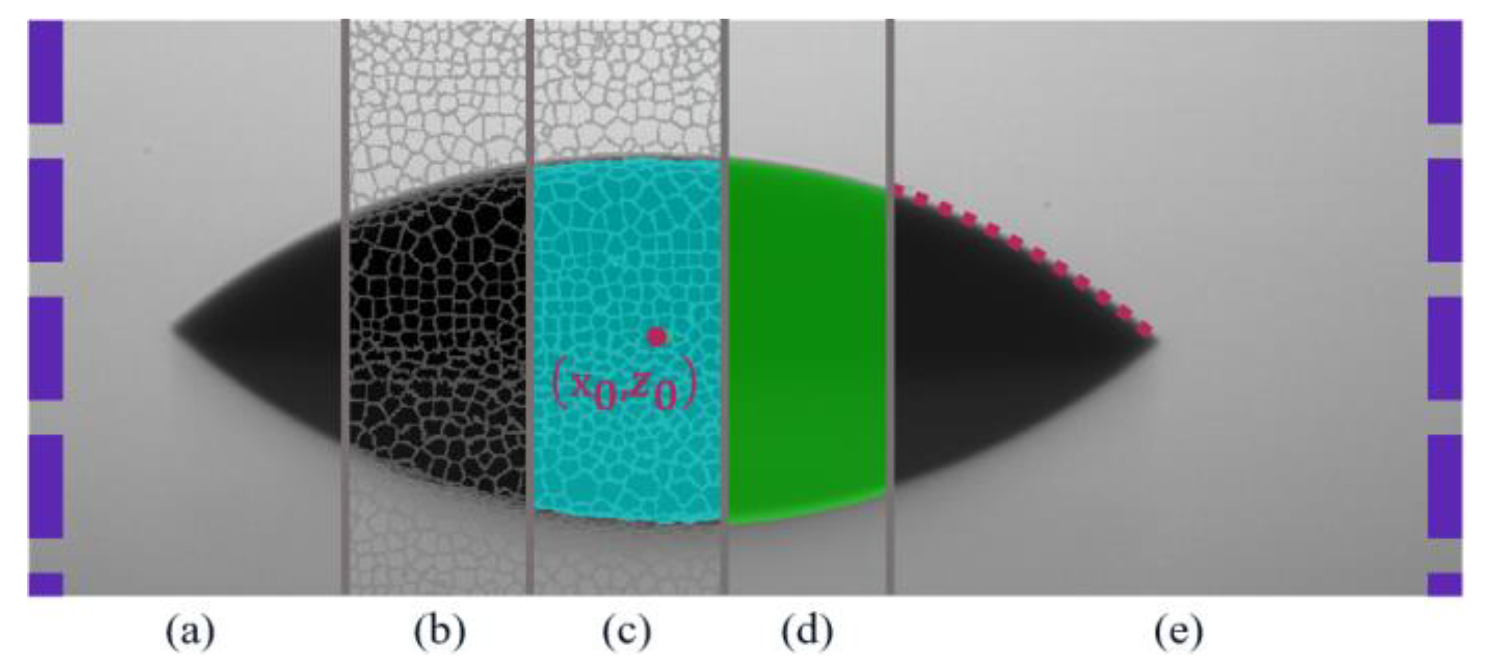
Figure 4.
Aligning centering and polar fitting of the extracted droplet contour. (a) Extracted contour in red and mirrored extended contour in green. (b) Polar plot of contour original in red, streched contour in blue. (c) Plot of stretched contour using angular position and radial distance. (d) Converted back to cartesian space and rescaled fit in cartesian coordinates.
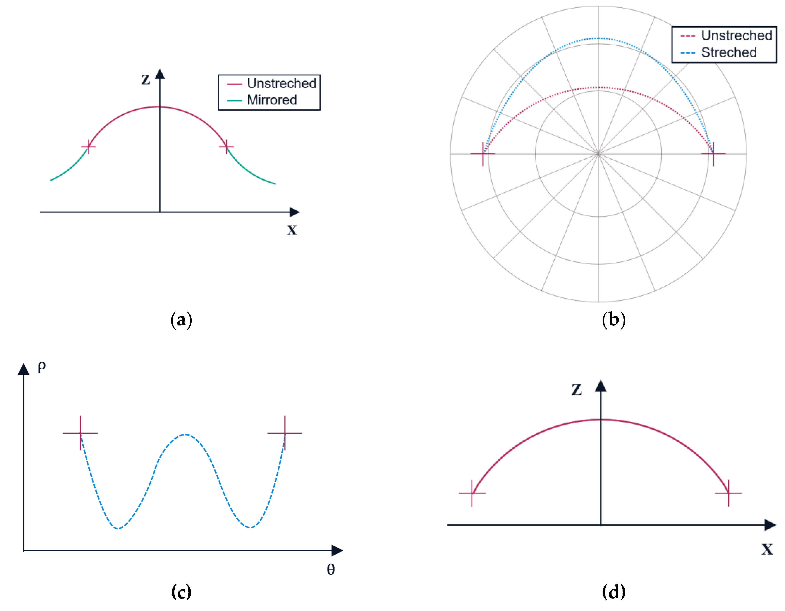
Figure 5.
Middle and PHDR (a) Midpoint calculation of x-slice. (b) Midpoint calculation of y-slice. (c) Aligned and scaled slices with points in one plane. (d) Curve interpolation using PHDR.
Figure 5.
Middle and PHDR (a) Midpoint calculation of x-slice. (b) Midpoint calculation of y-slice. (c) Aligned and scaled slices with points in one plane. (d) Curve interpolation using PHDR.
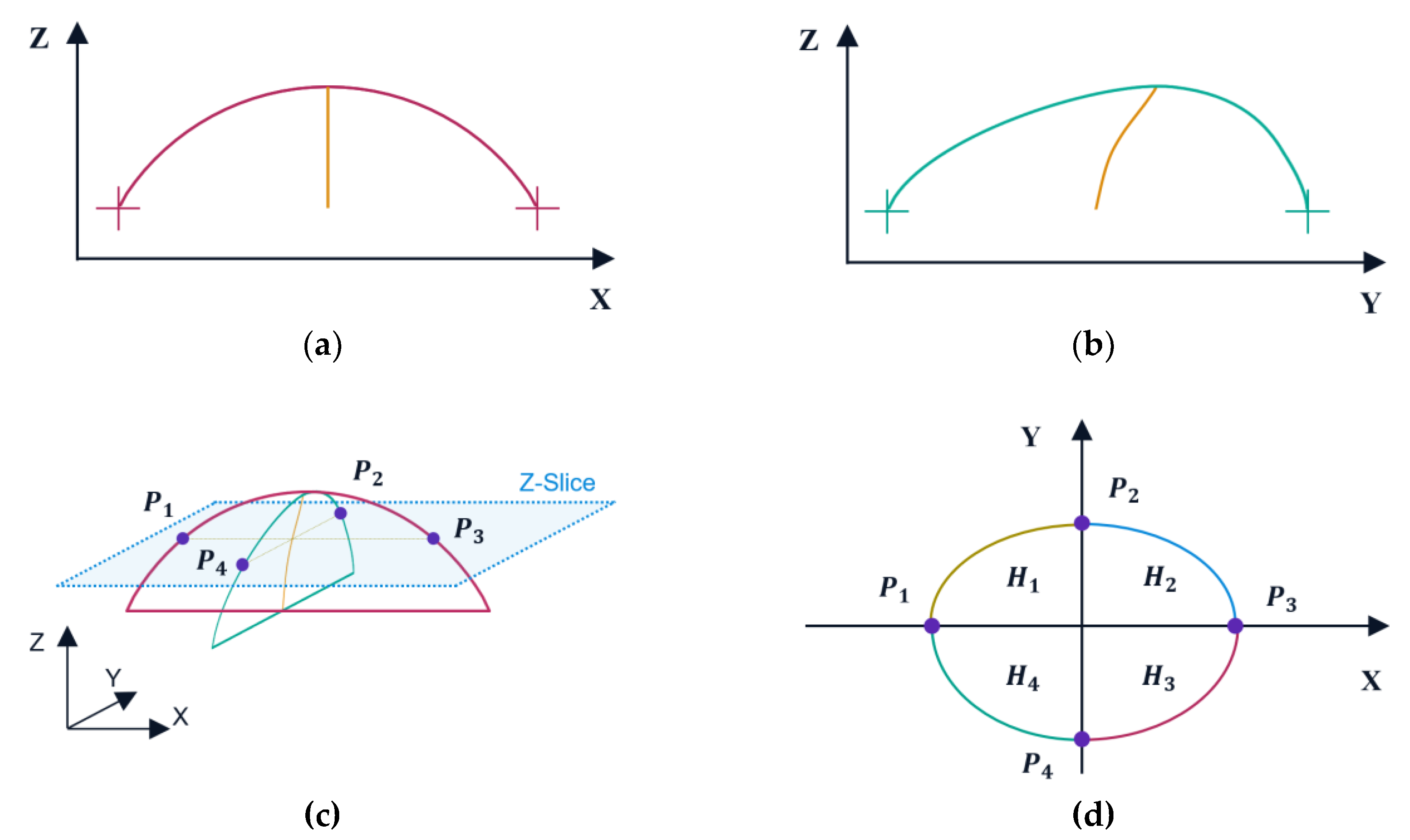
Figure 6.
Defining features of a nonaxisymmetric droplet.
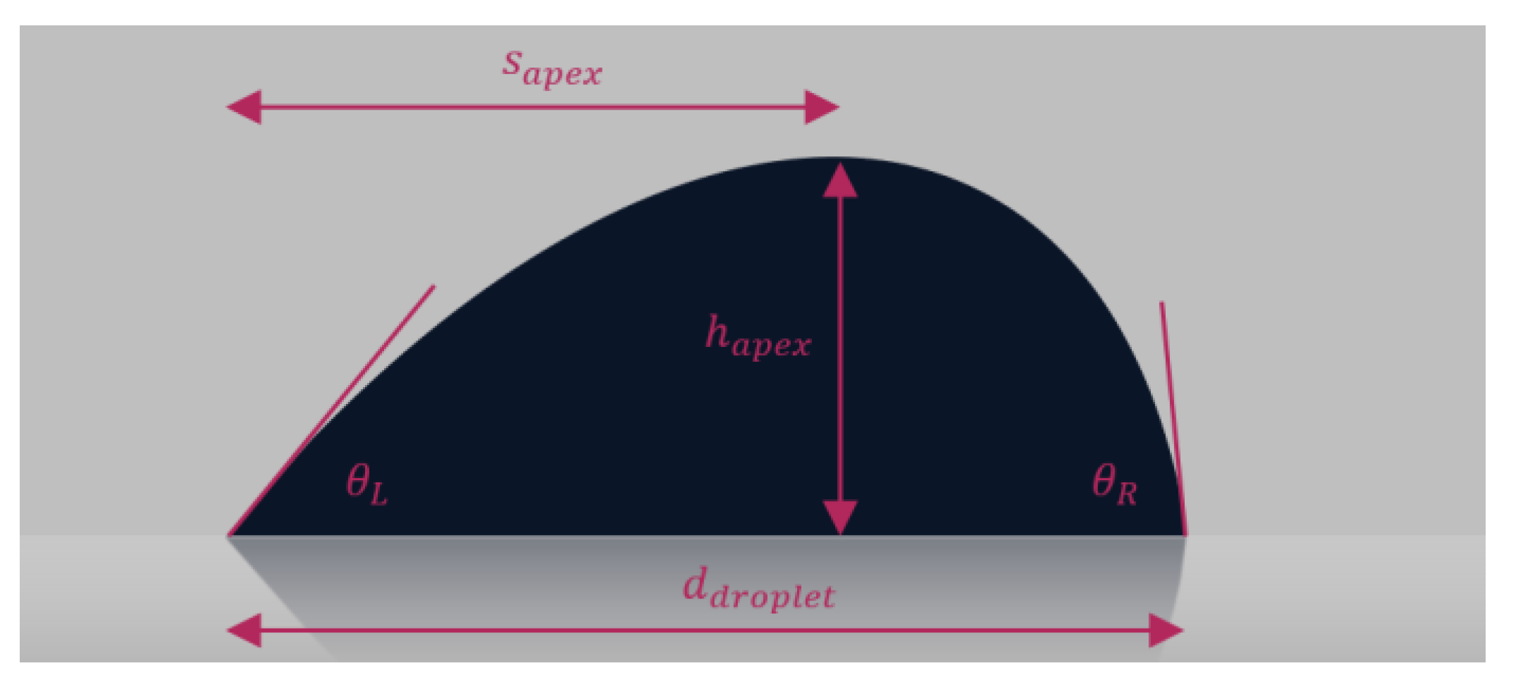
Figure 7.
Used synthetic curves with the real observed experiment image. (a) Circle shaped contour. (b) Hyperbola shaped contour. (c) Slanted hyperbola contour. (d) Rectangle shaped contour.
Figure 7.
Used synthetic curves with the real observed experiment image. (a) Circle shaped contour. (b) Hyperbola shaped contour. (c) Slanted hyperbola contour. (d) Rectangle shaped contour.
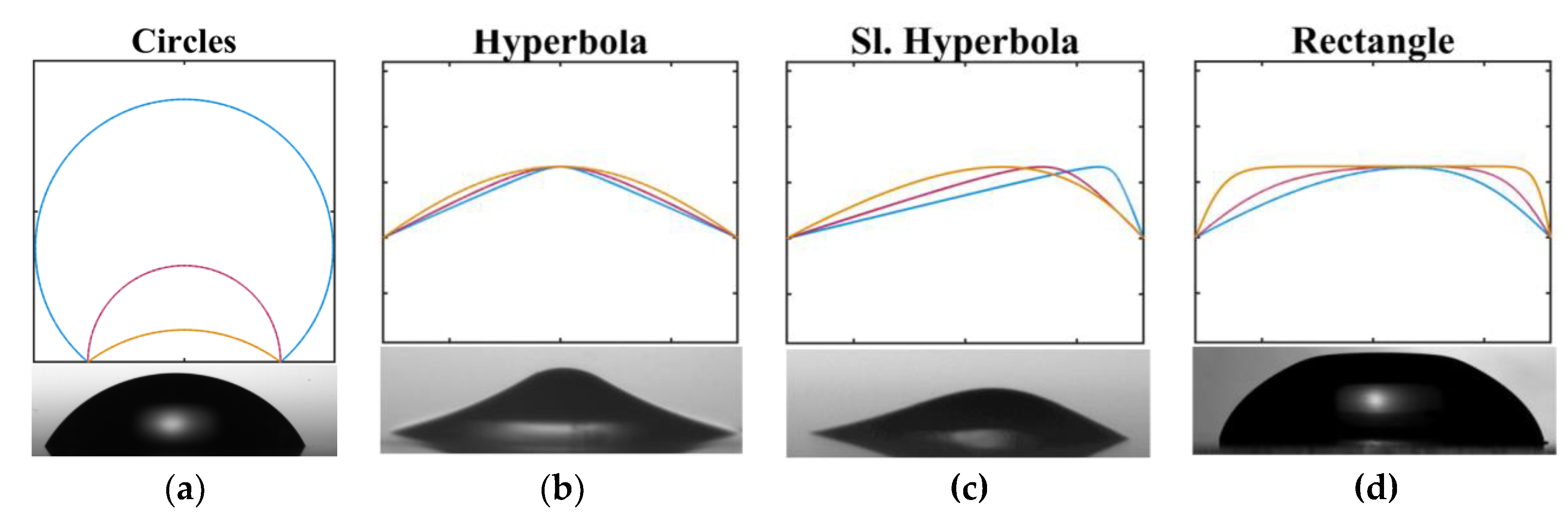
Figure 8.
Boxplots of circles, hyperbola, slanted hyperbola and rectangle measurements. (a) RMSE, (b) MAPE and (c) MNE.
Figure 8.
Boxplots of circles, hyperbola, slanted hyperbola and rectangle measurements. (a) RMSE, (b) MAPE and (c) MNE.
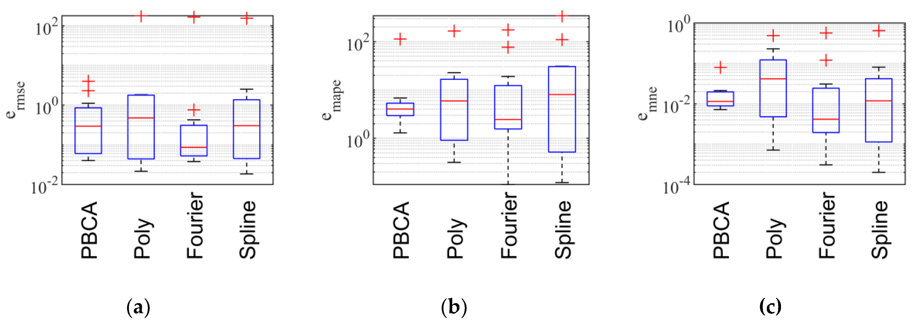
Figure 9.
Synthetic CAD models resembling droplets to test the 3D reconstruction and the top view of the Euclidean distances between ground truth and reconstructed model. (a) Semi sphere. (b) On axis deformed. (c) Off axis deformed. (d) top view of semisphere. (e) Top view of off axis deformation. (f) Top view of off axis deformation.
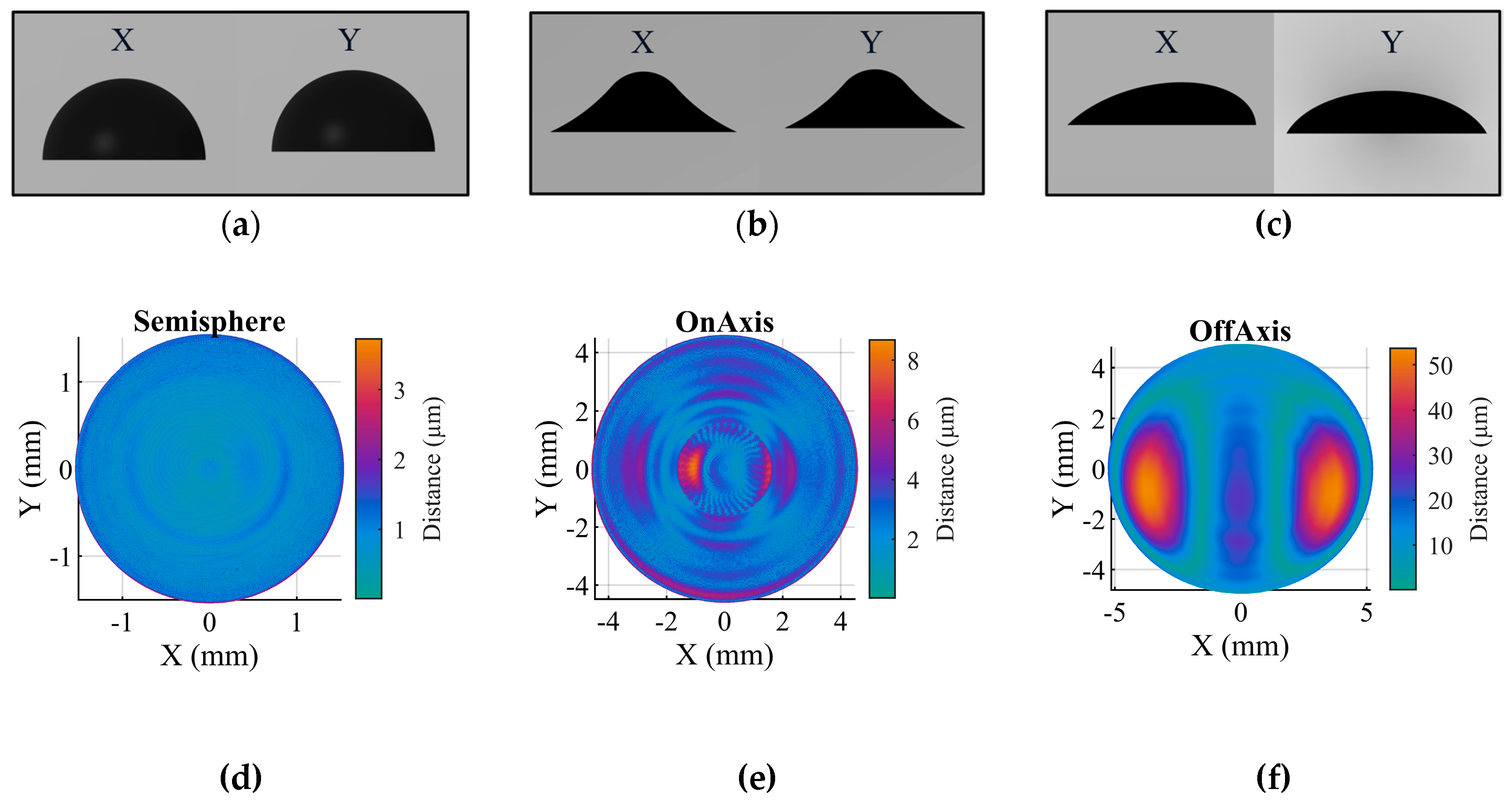
Figure 10.
Synthetic CAD models of extreme geometries reconstruction and the top view of the Euclidean distances between ground truth and reconstructed model (a) Pyramid. (b) Crooked pyramid. (c) Top view of pyramid. (d) Top view of crooked pyramid.
Figure 10.
Synthetic CAD models of extreme geometries reconstruction and the top view of the Euclidean distances between ground truth and reconstructed model (a) Pyramid. (b) Crooked pyramid. (c) Top view of pyramid. (d) Top view of crooked pyramid.
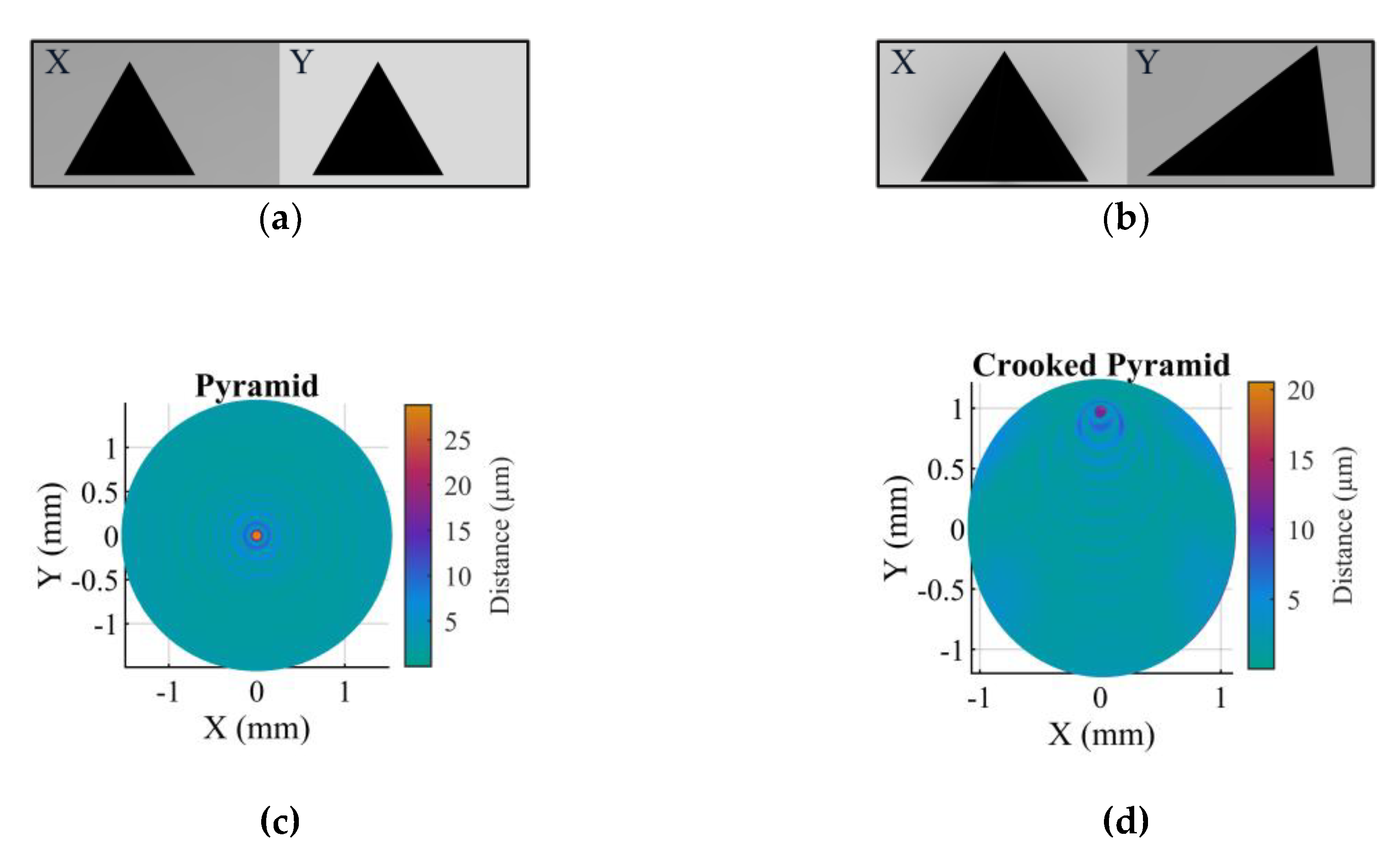
Figure 11.
Real X and Y images of precision machined pins and a CMM ball and the top view of the Euclidean distances between ground truth and reconstructed model. (a) Precision in with radius of 2.56 mm. (b) Precision in with radius of 3.63 mm. (c) Precision in with radius of 6.5 mm. (d) Coordinate measurement machine ball with diameter of 3 mm. (d) top view of.
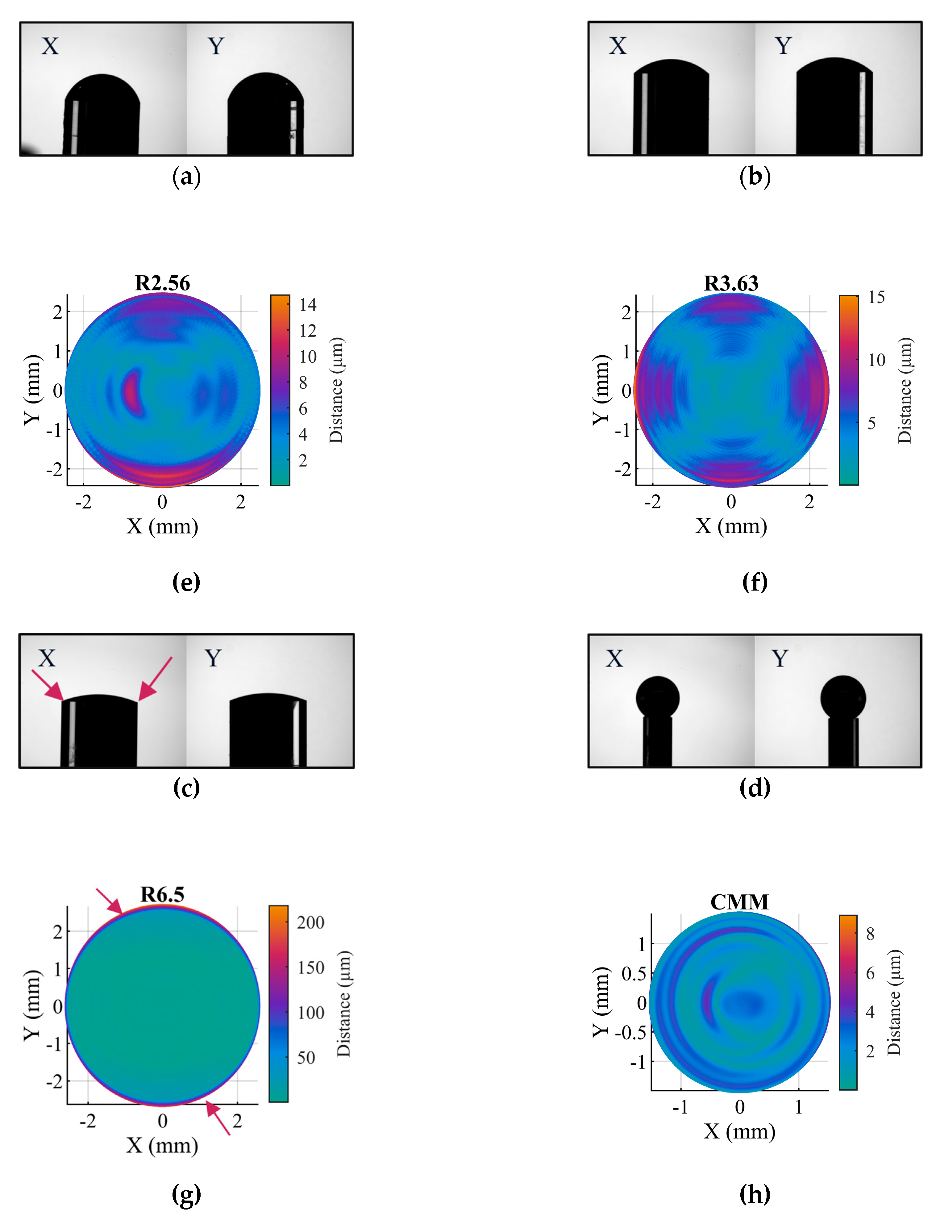
Figure 12.
a) Cmm ball in the setup. (b) Volume and Tenengrad measure for move on X-axis. (c) Volume and Tenengrad measure for move on Y-axis.
Figure 12.
a) Cmm ball in the setup. (b) Volume and Tenengrad measure for move on X-axis. (c) Volume and Tenengrad measure for move on Y-axis.
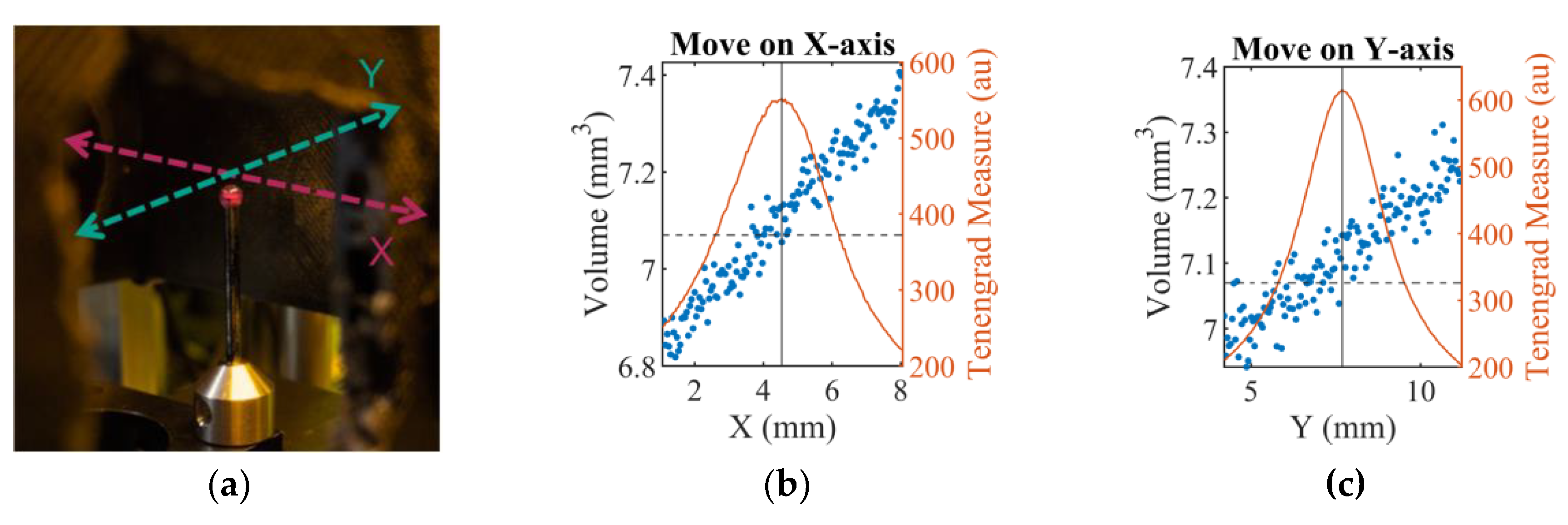
Figure 13.
a) Contact point random error. (b) Angles with random error. (c) Histogram of simulated volumes. (d) Boxplot of simulated volumes.
Figure 13.
a) Contact point random error. (b) Angles with random error. (c) Histogram of simulated volumes. (d) Boxplot of simulated volumes.
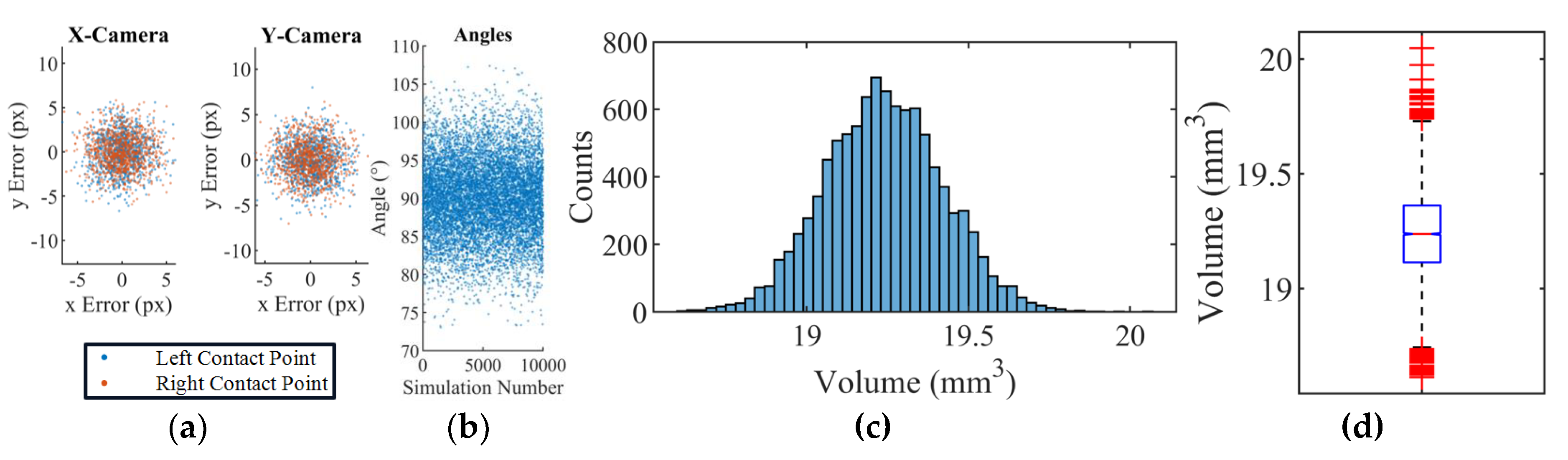
Figure 14.
a) Oleic acid on top of the pin inside the balance. (b) The anode used in the experiment. (c) X-camera image of the undeformed droplet in the setup. (d) Y-camera image of the undeformed droplet.
Figure 14.
a) Oleic acid on top of the pin inside the balance. (b) The anode used in the experiment. (c) X-camera image of the undeformed droplet in the setup. (d) Y-camera image of the undeformed droplet.
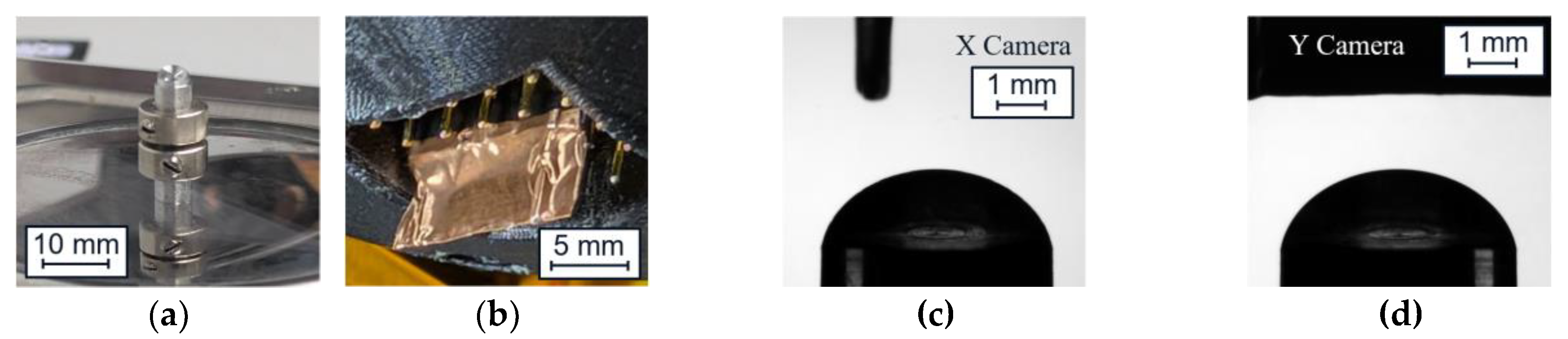
Figure 15.
Reconstructed volume of the experiment 5 over the course of the experiments.
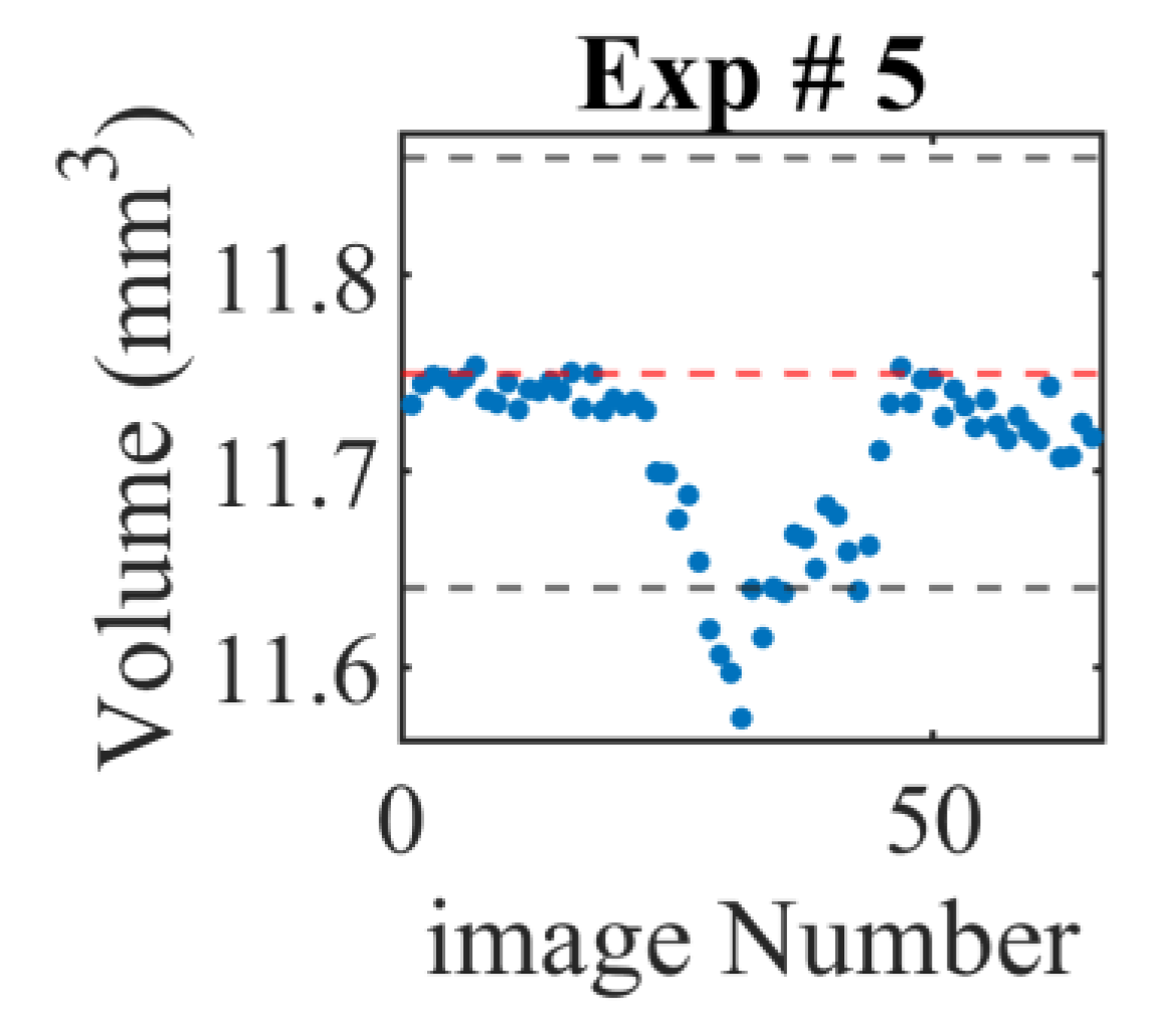

Table 1.
Control variables of the curves, values are in pixel.
| Line color | ||||||||
| Blue (1) | 494 | 50 | 300 | 50 | 150 | 50 | 50 | 25 |
| Red (2) | 319 | 150 | 300 | 100 | 150 | 100 | 50 | 25 |
| Yellow (3) | 533 | 600 | 300 | 300 | 150 | 300 | 50 | 25 |
Table 2.
metrics describing scaling of the images and the results.
| Semisphere | On axis | Off axis | |
| 7.07 | 61.5 | 99.89 | |
| 7.08 | 61.46 | 96.58 | |
| 0.01 | 0.04 | 3.31 | |
| 0.14 | 0.07 | 3.31 | |
| 1.05 | 3.19 | 21.16 | |
| Max distance (µm) | 3.72 | 8.7 | 53.7 |
Table 3.
metrics describing the CMM ball and the pins and the results.
| Pin 1 | Pin 2 | Pin 3 | Cmm | |
| 19.21 | 9.21 | 4.59 | 7.07 | |
| 19.19 | 9.21 | 4.60 | 7.02 | |
| 0.02 | 0 | 0.01 | 0.05 | |
| 0.1 | 0 | 0.22 | 0.7 | |
| 4.28 | 4.17 | 11.15 | 2.48 | |
| Max Distance (µm) | 14.36 | 14.47 | 292.05 | 9.76 |
Disclaimer/Publisher’s Note: The statements, opinions and data contained in all publications are solely those of the individual author(s) and contributor(s) and not of MDPI and/or the editor(s). MDPI and/or the editor(s) disclaim responsibility for any injury to people or property resulting from any ideas, methods, instructions or products referred to in the content. |
© 2025 by the authors. Licensee MDPI, Basel, Switzerland. This article is an open access article distributed under the terms and conditions of the Creative Commons Attribution (CC BY) license (http://creativecommons.org/licenses/by/4.0/).
Copyright: This open access article is published under a Creative Commons CC BY 4.0 license, which permit the free download, distribution, and reuse, provided that the author and preprint are cited in any reuse.


