
Submitted:
17 June 2025
Posted:
19 June 2025
You are already at the latest version
Abstract
The most common size measurements for agricultural produce, including fruits and vegetables, are length and width. While the length of any agricultural produce can be unique, the width varies continuously along its length. Single-width measurements alone are insufficient to accurately characterize the varying width profile, resulting in an inaccurate representation of the shape or mean dimension. Consequently, manual measurement of multiple and mean dimensions is laborious or impractical, and no information in this domain is available. Therefore, an efficient alternative computer vision measurement tool was developed utilizing ImageJ. Twenty sample sets, comprising fruits and vegetables, each representing different shapes, were selected and measured for length and multiple widths. A statistically significant minimum number of multiple widths was determined for practical measurements based on object shape. The “aspect ratio” (width/length) was identified to serve as an effective indicator of the minimum multiple width measurements. In general, 50 multiple width measurements are recommended; however, even 15 measurements would be satisfactory (1.0±0.6 deviation from 50 widths). The developed plugin was fast (734±365 CPU time/image), accurate (>=99.6%), cost-effective, and incorporated several user-friendly and helpful features. The study outcomes have practical applications in characterization, quality control, grading and sorting, and pricing determination of agricultural produce.
Keywords:
fruits and vegetables
; grading and sorting
; horticultural crops
; imageJ
; image processing
; physical properties
; quality control
1. Introduction
Length and width form the most common size measurements that characterize agricultural and horticultural produce. Size significantly impacts the external appearance of fruits and vegetables, as the price of produce generally correlates well with its size [1]. With agricultural produce, such as fruits and vegetables, the object will have a unique length but will have several varying widths along the length. A single width measurement will not provide the best description of the object’s width profile. However, the most reported dimensions are from a single measurement per object.
For example, using the computer vision image analysis “pixel-march” method [2] measured the orthogonal length and width of agricultural produce. Therefore, multiple widths will only describe the shape of the object better, and a correct representation, or at least a mean width derived from the multiple widths, would provide a better description.
While dealing with axisymmetrical objects, which have rotational symmetry about their length, the width measurement will also depict the thickness (orthogonal to the width and length). Such measurements will provide the best description of the product shape based on simple orthogonal dimensions. Most agricultural produce and products belong to axisymmetrical (convex) shapes, while non-axisymmetrical (concave or curved) shapes occur in agricultural produce, but they are less prominent and are not considered in this study.
In the grading and sorting of agricultural produce, the size constitutes one of the primary criteria, while other factors such as shape, color, and surface defects are also considered. Manual measurement, which is the known and common method, becomes laborious, tiresome, subjective, and prone to inaccuracy and reproducibility issues.
Several machine-based grading or sorting systems have increasingly been adopted in the industry to address these limitations. These systems utilize computer-based algorithms to analyze digital images and interface with activating mechanisms that perform the actual separation or sorting process.
Computer/machine vision systems have been used increasingly in these industries and food processing plants due to their ability to provide rapid, cost-effective, hygienic, consistent, accurate, and objective assessment, online automatic process control, and real-time quality evaluation [3,4]. In addition, computer vision image analysis applications are well established and proven successful for classification, volume and mass estimation, defect detection, size and shape features measurement, quality inspection, and grading of grains, fruits, and vegetables in agricultural and food process engineering fields [5,6,7,8,9].
Reviews on computer vision or image processing are available applicable to quality evaluation, size and volume determination, shape analysis of fruits and vegetables, agricultural products, and food products [1,4,10,11,12,13], and developments in these fields [14], illustrate several applications to agricultural produce and products. A latest review describes the basic method (capliper) to the modern method (machine vision and deep learning) for size assessment of fruit on trees in the orchard directly [15]. In addition, some novel applications of image processing include the determination of volume and surface area of agricultural products [16,17], and major orthogonal dimensions measurements of food grains [2]. Relationships between volume and mass of axi-symmetric fruits like apple, sweet-lime, lemon, and orange were estimated using an imaging technique with five different views of a fruit and geometrical formulas [18]. Machine vision-based systems were employed for in-line sorting, detection of contaminants or specific chemical compounds on the product?s surface [19]. Object detection and depth maps with a stereo camera for vegetable (cucumber, eggplant, tomato, and pepper) recognition and size estimation using six keypoints [20].
Recently, fruits and vegetable disease recognition using convolutional neural networks and YOLO deep learning modles [21], three-dimensional (3D) machine vision techniques have been widely employed in agriculture and food systems, utilizing modern 3D vision systems and advanced deep learning technologies [22,23], application of computer-vision-based industrial algorithm for the detection of the dimensions and the spatial positioning of fruit and vegetables on a conveyor belt for their movement to a packing machine with a robotic arm [24], and several similar research outputs have been reported. In a modeling study, models for the non-destructive in situ detection of individual fruit mass in diversely shaped tomatoes from the greatest width and length [25].
Computer vision techniques and image analysis make it possible to obtain these lengths and multiple widths automatically. Recognizing the significance of multiple widths in representing actual profiles and deriving the mean width, it is pertinent to assess the variation of width along the length and determine the number of multiple widths required to represent a statistically significant mean width. Despite these state-of-the-art systems making significant advancements, particularly in complex tasks such as identification, classification, object localization, handling occlusions, robotics, and overall shapes and dimensions; no reports on these aspects of multiple dimensions measurement of agricultural produce, mean width, and statistically significant least number of multiple measurements were found in the literature. Thus, making this research necessary, significant, and unique.
Our goal is to create a method, measure the multiple widths of axisymmetrical objects such as agricultural produce, and find out statistically how few multiple widths are needed to represent them accurately. Therefore, the objectives of this research are to (i) develop a computer vision analysis tool utilizing the open-source ImageJ analysis platform (ImageJ plugin) to process the digital images and validate the algorithm; (ii) apply it to measure the length and orthogonal multiple widths of several axisymmetrical agricultural produce; (iii) determine their mean width and the least number of statistically significant multiple widths; and (iv) statistically evaluate the effect of number of multiple widths on the mean width.
2. Materials and Methods
2.1. Test Material
The test material used in this study was agricultural produce (vegetables and fruits) obtained from the local grocery stores. Pasta fettuccine, carrots, celery, green beans, potato, and sweet potato were obtained from Bismarck and Mandan, ND, USA, and the rest of the fresh produce from Coimbatore, TN, India. Original images of these 20 selected test materials used in the study, along with a sample multiple measurement width results, can be found in the “Mendeley Data” repository (https://doi.org/10.17632/jprxshtr4t.1) [26]. A montage of these image samples is presented in Figure 1 for illustration.
The selected agricultural produce samples were axisymmetrical, characterized by uniform widths and thicknesses along their length. Axisymmetrical shapes produce near-circular cross-sections perpendicular to the rotational length axis. In addition, axisymmetrical objects mostly belong to convex shapes, where the centroid of the projected area lies inside the object itself; as opposed to concave shapes (curved or bent) that represent only a relatively small population among agricultural produce, where the centroid lies outside of the object’s projected area and complicates the measurement.
2.2. Overall Workflow of the Research Work
The workflow of the computer vision research on developing the user-coded ImageJ plugin for multiple width measurement for agricultural produce is presented in the form of a flowchart in Figure 2. Some of the processes depicted (Figure 2) should be understood in conjunction with the ImageJ environment and were achieved through the Java source code of the plugin, while others depict general setup, input, and output operations. Details of component processes are discussed as required.
2.3. Image Acquisition of Agricultural Produce Samples
Domestic digital cameras (1: Canon PowerShot, SX100 IS, 8.0 megapixel, 10X optical zoom, USA; and 2: Canon PowerShot, A3300 IS, 16.0 megapixel, 5X optical zoom, USA) were utilized to capture the test material images. The image size directly influences the measurement accuracy through the resolution of the images. A large image size usually defines the object with an increased number of pixels, resulting in increased resolution, thereby improving measurement accuracy. The resolution of the images is typically expressed in dots per inch (DPI; Figure 2), and the DPI information will be accessible from the image properties.
DPI of an image will vary depending on the focused distance (whether manual or autofocus) or the distance between the object and the camera. When the camera is positioned closer to the object, both the DPI and the accuracy of measurements increase. However, this proximity also reduces the “field of view,” thereby limiting the number of objects that can be captured within a single image. Conversely, maintaining a constant distance between the object and the camera does not affect the DPI of the images.
Fixing the camera on a stand in such a way that it aligns perpendicular and focuses on objects is a basic system suitable for laboratory and industrial settings. However, without securing the camera, images for practical use can be obtained by incorporating a reference object of known dimensions within the image frame. This reference object serves as a legend or scale, based on which the dimensions of the objects in the image can be calibrated and measured. There is no restriction in choosing the reference frame dimensions, but it should be proportionately larger than the tested objects and exhibit contrasting colors with the object, so that the profiles of the object are correctly captured. In this study, a “Thermocol board” measuring 1.0 0.5 and a “letter paper (US)” with a drawn rectangle of dimension 242 mm × 178 mm (Figure 3) were utilized as the reference frames.
Images were captured in a manner that the reference frame occupies the major area of the picture at the highest possible resolution. Objects were arranged so that they do not touch one another (singulated arrangement), and the orientation of objects without protrusions (e.g., pedicles) does not matter. Special roller or chain conveyors presenting fruits individually (singulated) for machine inspection or other operations are common in the industry. However, produce with pedicles should be arranged so that all faces one direction (Figure 1: Eggplant samples), as these components were ignored from measurements using the “end caps” methodology coded in the plugin.
Shadows of the objects should be avoided as they will be included in the projected object area during preprocessing if the object color matches the shadow color. Indirect or diffused lighting, as well as multiple lighting sources, can effectively eliminate shadows. Images captured using natural lighting in shaded areas or with multiple fluorescent lights tend to yield good results. In the case of small objects, such as grains and other particulate materials, a document scanner proved to be an efficient imaging tool [2]. The scanner provides the best lighting without shadows, along with very high resolutions (DPI ). Scanners can be readily utilized for small-sized produce (e.g., berries, grapes, nuts).
2.4. Computer Vision Image Analysis Framework Used
The developed computer vision image analysis plugin utilizes the Java language and Fiji (Ver. ImageJ 1.54p; http://fiji.sc/Fiji) package. Fiji is an image processing package and is a distribution of ImageJ, an open-source, free image analysis program [27,28]. It is quite popular among scientists working with biological imaging [29]. Fiji is a feature-rich integrated development environment of ImageJ that offers various commands for plugin development [30]. Researchers have developed custom-made ImageJ plugins to address diverse computer vision applications. Some of the examples are food grains dimensions [2]; morphological characterization of particles [31]; blood vessel diameter measurement [32]; and several more. These plugins played a role in advancing scientific research in these areas.
2.5. Image Preprocessing
In computer vision image analysis, the fundamental calculations are initially performed on pixel units, and subsequently, these values are converted into practical physical units. The calibration process establishes a correlation between the pixel values and the physical dimensions of the object. In most image processing algorithms (Figure 2), the binary image gets handled easily and is used to derive various standard parameters from the image processing programs. Therefore, color images were initially converted into binary images (black and white colors only) using the image processing system. The ImageJ’s “8-bit” and “Threshold…” commands created the grayscale and binary images, respectively. The information displayed in typewriter font (e.g, “8-bit”) refers to actual ImageJ commands.
The DPI information (pixel values of a reference object) of the image can be extracted by tracing the known reference rectangular frame or line using the “Rectangular” or “Straight” selection tool, respectively. From the `w’ (width) and `h’ (height) or the `l’ (length) of the reference frame or line in pixels, the DPI of the image is calculated as follows:
The measurement resolution (the smallest dimension that can be measured) can be obtained from the DPI as follows:
Once the image DPI is measured and recorded (Equation (1)), the image can be cropped, if necessary, to only include the objects while eliminating the unnecessary background details, since image cropping preserves the DPI. Fine particles, such as dust or other specks, can be omitted from analysis by setting the “Analyze Particles …” area range from the “Size (pixel⌃2)” to a minimum cutoff value. This minimum cutoff value depends on the projected area of the object and the DPI of the image. For instance, the smallest object, namely the ivy gourd image (Figure 1) at 109 DPI had the object projected area ranging from 10,635 to 31,; thus, a “Size (pixel⌃2)” input of “10000-Infinity” will eliminate small and fine particles for the entire set of samples studied. However, if the objective is to remove only the dust and small non-objects, a smaller range, such as “1000-Infinity” (≈1/10 of the minimum area), can also be employed to ensure the inclusion of larger objects.
During actual measurement, filtering can be performed, or an image mask can be obtained by eliminating the finer particles beforehand. It is essential to check the “Exclude on edges” and “Include holes” options of “Analyze Particles …” while making the mask to ensure that the entire area of the object gets completely filled. Any partially cropped object will be discarded.
2.6. Plugin Development and Description Of Methodology
A brief description of the developed multiple and mean width measurement plugin (Figure 4) and its methodology is described hereunder. The plugin consisted of about 1250 lines of Java code (including comments) and employed several Java methods to execute its functionalities. These methods include the following activities: (i) Initial setup that derives the standard ImageJ output of particle analysis, (ii) determining the length and width limits of objects, (iii) reading user inputs based on object properties, (iv) evaluating multiple and mean widths, as well as lengths, and visualizing these measurements on a binary image, (v) logging the individual multiple width measurements for each object, (vi) summarizing the overall results for all objects, (vii) creating separate graphs of multiple widths for each object based on user inputs and orientation, and (viii) exporting the output as a consolidated CSV file for all measuring sessions.
2.6.1. Plugin’S User Input Front Panel
The plugin’s user input front panel presents a suite of inputs to perform various activities and achieve the desired results (Figure 4C). The input panel has several numeric field text boxes and boolean-valued check boxes to facilitate input collection. Several of these choices were coded as default, allowing the plugin to run without users’ intervention if the defaults suit their requirement or for a trial run. In alternative cases, users can provide their specific inputs and obtain the desired outputs.
The calibration (pixel to physical dimensional units conversion) process can be performed either through the DPI value or the reference frame dimensions. As previously described (Section 2.5), when the known DPI value of the image (Equation (1)) is combined with a binary mask, the calibration can be performed directly (Figure 4C). Conversely, if DPI is not known, the number of pixels that constitute the reference frame can be used for calibration (Figure 4C). Both these methods result in the conversion of the pixel values into physical dimensions (mm). If the image title contains DPI values, the plugin will process the text, extract the DPI values, and populate them automatically. We followed this approach to have the DPI value in the image titles to enable this automatic reading and better documentation of images.
It is common practice in the cultivation of vegetables and fruits to harvest some produce with pedicles intact. These pedicles can interfere with the multiple width measurement, since any measurement of width along the pedicles will not be representative of the economically important portion of the produce. To tackle the presence of the pedicles, the “end cap” chopping methodology was incorporated (Figure 4C). As the images were read from “left to right” and “top to bottom,” the end cap values should be input accordingly. Therefore, left- or top-oriented pedicles should result in higher top end chop percent values compared to the bottom, and vice versa. As the end chop values are applied uniformly in a session, it will be prudent to orient the sample with the pedicles pointing in a way so that a single end cap value can be applied to all the objects in the image (Figure 1: eggplant shot pink and eggplant long green). Future developments should aim to automatically identify the pedicle and apply the end cap values correctly, regardless of their orientation.
One of the other analysis inputs (Figure 4C) is the desired number of multiple width measurements. A suggestion, based on 80% of the smallest length of the object, was also indicated, and any value equal to or less than this limit can be used. In this research, it is intended to find the optimum number of width measurements beyond which no statistical difference will be observed. Also, a default value of 50 was provided for the user. The final input box gives another chance of filtering out the small particles based on the area, expressed in the number of square pixels. A default value of 10 was set and can be modified by the user.
The output-related selections can be exercised through the checkboxes: (i) multiple-width drawing output on a binary image of the object to visualize the measured locations of the widths (Figure 4E); (ii) multiple-width results in the form of a “Log” window for immediate consumption (Figure 4G); (iii) multiple-width visualization as a graphical plot for each object in the image (Figure 4D); and (iv) multiple-width graphical plot orientation (the swapping of x and y axes to visualize the plotted width as desired by the user (Figure 4E). As a background task, all the consolidated results of all measurement sessions will be appended to a CSV file for recording and documentation.
2.6.2. Methodology of Multiple Widths and Length Measurement
Utilizing Fiji as the plugin environment (Figure 4A), the “pixel-march,” as reported elsewhere [2], seeks black pixels while marching along the white pixels, following the specified straight line paths, to evaluate both length and widths. For this purpose, it is essential that the interior of the object be continuous and filled with white pixels, which is ensured by the “Include holes” (Figure 4B). Convex-shaped objects ensure that the centroid (Figure 4E: 1), which serves as the starting point of the pixel-march, remains within the object’s outline, allowing the process of length and width measurements to proceed uninterrupted. If the centroid falls outside, determined based on the background color, only that object is excluded from the measurements. With the desired number of multiple widths, the “step-length” of segments for multiple width measurement was determined.
Based on the end caps chopping values, the segment length was calculated from the object length less the end caps length (Figure 4C). Different or similar end cap values can be used depending on the type of agricultural produce (e.g., with or without pedicle). Starting from the centroid, the widths were determined by finding the boundary pixels orthogonal to the length on both sides and using the distance formula. The widths were determined starting from the centroid and moving away towards both ends based on step-length (Figure 4E) for correct evaluation, but re-allotted from bottom/left to the top/right for plotting the widths (Figure 4D). The mean and standard deviation (STD) of multiple width measurements were calculated for each object. The length of the object was obtained along the major axis and through the centroid (Figure 4E). Textual results were produced for reading (Figure 4F) and for further statistical analysis in the form of a spreadsheet.
2.7. Statistical Analysis of Multiple Widths
It is of practical interest to investigate the effect of the number of widths to be considered and their statistical significance, and the mean separation analysis results that provide such insights. Several multiple widths ranging from 1 to 200 were considered, with measurements chosen closely towards the smaller numbers. The effect of the number of multiple widths on the measured mean width and its statistical significance was evaluated using the mean separation method (pairwise differences among means). A SAS (Ver. 9.3, 2009, SAS Institute, Cary, North Carolina, USA) macro %mmaov that used PROC MIXED [33] performed the mean separation analysis. This macro converts the means pairwise differences to letter groups, where means that share a common letter are not statistically different at a specified level. The macro was run with mean width as the dependent variable; produce name, and number of multiple widths measured as classification and fixed variables; logarithmic data transformation a common technique to reduce skewness in the data and make it more normally distributed, meeting the normal distribution assumption used in the analysis); grouping by produce name; ; and adjustment by Tukey.
3. Results and Discussion
For the agricultural produce images captured in this study from the digital camera, the DPI values were within the range of 109 and 246, resulting in a measurement accuracy or resolution (Equation (2)) of 0.103 to 0.233 mm pixel−1. Increased DPI values are feasible with high-resolution cameras. A DPI of 600 (0.042 mm pixel−1) or more is quite common with digital scanners. Therefore, based on the necessary measurement accuracy, the appropriate image resolution (DPI) should be selected.
3.1. Features of Developed Plugin
Several features are built into the developed plugin and are briefly described below. The plugin accommodates two calibration methods, namely, DPI and reference dimensions input (Figure 4C). However, in a fixed setting with a stationary camera where the distance between the objects and the camera remains constant, the calibration values can be directly coded into the plugin, eliminating the calibration routine. The plugin extracts the object name and DPI value from the file name of the image using Java string processing commands if the information is included in the specified pattern. This extracted DPI value gets filled in the “Use DPI” input box of the plugin input panel for ready execution (Figure 4C), and the object name is used for results output.
The plugin (Figure 4) is capable of analyzing images containing objects in any orientation. Consequently, the multiple widths measured were made to orient orthogonal to the major axis of any inclination. In addition, the top and bottom end caps chopping values can be input individually to preferentially address the presence of pedicles and exclude them in multiple width measurements (Figure 4E). The plugin identifies concave objects (centroid falling outside of the profile) and outputs a message with the identification label number to facilitate their elimination through further preprocessing and rerun. For example, the 5th object from the left on the color image of green beans (Figure 1: Green bean) has a highly curved shape, indicating it is a concave object, and it is removed from the binary image for measurement purposes [26].
The plugin generates various textual, data, and graphical forms of outputs (Figure 4). Usually, the results are displayed in the “Log” window, showing the overall results (Figure 4F,H), and individual multiple-width results (Figure 4G) can also be produced. The plugin also directs consolidated results and continuously archives them to an external spreadsheet through a CSV file format. Graphical outputs include visualizations of measured widths as plots (Figure 4C,D) as well as drawings of widths and length directly on a binary image (Figure 4C,E).
The developed measurement methodology is cost-effective as it requires only an inexpensive domestic digital camera and the necessary plugin created using an open-source and free Fiji ImageJ software. Thus, the investment for the system rests on the digital camera (e.g., 48-megapixel ), and the supplementary lighting supplies. However, a practical unit that incorporates this algorithm and associated hardware for grading or sorting may require additional costs for scaled-up operations.
3.2. Plugin Validation
The validation of the plugin can be performed by analyzing an image (without a reference frame) that contains objects of known dimensions. An image depicting directly drawn rectangles and precision-cut paper strips of known dimensions (Figure 5), was analyzed using the plugin, and the results are tabulated (Table 1). The objective is to test the plugin’s performance by conducting multiple measurements with simple reference objects. It is also possible to use several standard precision objects for the plugin performance test as alternatives.
Results indicate that the plugin correctly measured drawn blocks on the image with perfect edges (Table 1), and the length and multiple widths have great measurement accuracy (99.98%–100%). This demonstrates the capability of the plugin to make exact measurements when images with clean outlines are used. However, the cut paper strips’ length and multiple widths accuracy ranged from 95.70% to 99.25%.
The results demonstrate that the plugin accurately measures drawn blocks on images with precise edges, as evidenced by the high measurement accuracy (99.98%–100%) for length and multiple widths. This capability is particularly evident when using images with clean outlines. However, the accuracy of measuring the length and multiple widths of cut paper strips varied, ranging from 95.70% to 99.25%. These results are comparable to the absolute deviations (1.44%–2.15%) of computer vision analysis using a document scanner (300 DPI) observed with digital caliper dimensions of standard printed circuit board nylon spacers [2].
In the present study, the accuracy reduces as the strips become thinner (5 mm), as the number of pixels describing such widths diminishes, and individual pixels have a greater influence on the measurements. With a DPI of 256, each pixel represents 0.0992 ≈0.1 mm. This means exclusion/inclusion of a single pixel on a 5 mm reference width results in a loss of accuracy. However, on a 20 mm reference, this is linearly reduced to a accuracy loss, and further diminishes with increased dimensions.
As most of the practical samples are wider than thin 5 mm, a second experiment included a few wider samples made from letter paper (US; 215.9 mm × 279.4 mm) in validation (Table 1) at two resolutions. These wider strips even at 0.154 mm pixel−1 (165DPI) produced accuracies . With the increased resolution of 0.096 mm pixel−1 (265 DPI), the measurement accuracies further improved to . In addition, a whole letter paper (US), involving no manual cutting, identified as objects numbered 13 and 14 (Table 1) was validated at 165 and 265 DPI, and this showed a slight increase in accuracy with an increase in DPI. Thus, increasing DPI becomes a simple way of improving the measurement accuracy. Overall, the measurement accuracy of the plugin varied from 96% to 100%, and it improved with the resolution of the input image.
3.3. Multiple Width Results of Agricultural Produce
An example of multiple and mean dimension measurements, with papaya (Figure 1l) as an illustration from the agricultural produce studied (Figure 1), is presented in Figure 6. The original color image (Figure 6A) was duplicated to make a binary mask, in preprocessing stages, on which the length and multiple widths are measured and drawn (Figure 6B). The plugin was run with the loaded binary of the papaya and default values (DPI from image = 109, both end chop % = 10.0, and number of multiple widths = 50) of the plugin (Figure 4C) with some user inputs (uncheck rotating the profile). The length and multiple widths of each sample of the papaya image were plotted and labeled (Figure 6B).
The samples were identified from top to bottom and left to right (3rd papaya identified as 1st). The angle of inclination of the length direction (along the axis of the papaya) also represents the orientation of the object. The multiple widths were measured and drawn perpendicular to the length axis (Figure 6B). Measured multiple widths can be visualized through unrotated profile plots (width on x-axis and multiple width numbers on y-axis; Figure 6C). The unrotated multiple width plot also aids in visualizing the profile of the object as measured from bottom to top. The plugin also calculates the minimum, maximum, mean, and STD values of the multiple widths of all the objects in the sample image (Table 2).
Dimension measurement results for pasta fettuccine and 19 agricultural produce (Figure 1) are presented in Table 2. Length is a unique measurement for each sample, while 50 multiple width measurements were conducted for each sample used in the results illustration. Consequently, within each sample group, there will be distinct minimum and maximum lengths, whereas each sample will have a minimum and maximum width (based on 50 width measurements). The standard deviations are applicable only to the mean length and all three width values (Table 2).
The details presented in the supplementary material data [26] of the selected produce (Figure 1) show the cropped color image, the measured and labeled binary image, and a multiple-width plot of a selected sample that was identified from the plot title (e.g., n = 5). The plugin identifies objects by finding their topmost pixel while scanning from left to right, starting from top to bottom. For example, in the “Bitter gourds” (Figure 1b) sample set (Data [26], page 2), the natural first left sample is actually identified “9” as its top tip is lower than the other eight samples. This naturally left the first sample of the image selected for multiple-width plot visualization, and this number can also be identified from the title of a block of the plot “(n = 9).” These plots are for a single sample in the image, and similar plots for the rest of the samples were produced (plots not shown). The multiple width plot is a collection of caliper widths (Figure 4E-5) from bottom/left to top/right. This multiple widths plot clearly shows the width profile of the test samples, and a single value cannot able to specify this existing variation. The plugin accurately captures multiple width profiles and enables us to visualize the width variations (Data [26]).
The multiple-width profiles closely resemble the tested sample’s natural profile (Data [26]). For instance, pasta fettuccine (Figure 1a), a manufactured food product with uniform dimensions, exhibits a linear profile with minimal variation (mean around 4.7 mm). Bitter gourds (Figure 1b), on the other hand, demonstrate the zigzag profile characteristic of the sample’s rough surface. Carrots (Figure 1d) and celery (Figure 1e) exhibit a linear but inclined profile following their triangular or truncated pyramid shape. Green beans (Figure 1i) display a wavy pattern that accommodates the presence of seeds within the pod. Eggplants long green (Figure 1g), exhibit a typical inclined and curvilinear variation for a hook-shaped sample. Pineapples (Figure 1m) produce a linear profile with minimal variation as the fruit is cylindrical and rectangular in profile. The remaining produce exhibits a smooth dome-shaped profile, reflecting the spherical or prolate spheroid shape of the samples. Furthermore, any dent or deformation in the profile of the samples (e.g., potato [Figure 1n], snap melons [Figure 1p], sweet potato [Figure 1q]) was also captured. These findings clearly demonstrate the necessity of multiple width measurements to accurately measure the varying dimensions and visualize the actual profile or shape of the agricultural produce.
The aspect ratio shape factor () aids in identifying the sample’s elongation (smaller value) or roundness (higher values close to 1.0) (Table 2; Data [26]). Elongated samples, such as pasta fettuccine, green beans, carrots, and celery hearts, exhibited aspect ratios of 0.06, 008, 0.11, and 0.12, respectively. Conversely, round samples, including mangos, watermelons lightgreen, watermelons darkgreen, and snap melons, had the larger values of 0.88, 0.73, 0.70, and 0.62, respectively. It is important to note that these aspect ratio values are derived from the multiple width measurements and cannot be precisely obtained from simple single measurements.
3.4. Effect of Number of Width Measurements and Significance
The presence of multiple mean groups with samples (identified by uppercase letters; Table 3), except for pasta and celery, reinforces the necessity of multiple width measurements statistically ( = 0.05). The aspect ratio effectively served as an indicator of shape (Table 2) to determine the number of significant groups of multiple widths (Table 3). A smaller value of indicates an elongated object (e.g., pasta fettuccine, carrot, celery [Figure 1a,d,e, respectively]; ≤ 0.12), while an increased value suggests a more spherical object (e.g., mangoes, turnips, watermelons [Figure 1k,r,s and t, respectively]; ≥ 0.66). Overall, for 0.06 ≤≤ 0.12, the number of distinct mean groups was , while for increased > 0.2 the number of distinct mean groups was for most produce. Therefore, based on the , the number of multiple widths will be statistically different from the single width, and this difference diminishes with a reduction in and vice versa.
The minimum number of statistically significant multiple widths and the next below significant width tabulated (Table 3) as “#SigWidths” in the form: a⇔b, which illustrates the importance of multiple width measurements for sample shapes that deviate from linear profiles. For example, bitter gourds (Figure 1b) have 5 letter groups (A to E), but multiple widths of 10 through 200 are not significantly different. The first three widths (1 through 5) are all significantly different; widths from 7 through 25 are not significantly different, but widths 7 and 50 are significantly different. Working from the top after multiple widths 50, increasing the number of multiple widths beyond this limit does not produce a significant difference in mean widths; however, below this limit, 7 is the largest significantly different number (a⇔b = 50 ⇔ 7 in Table 3). Depending on the shape () wide variation on multiple widths (excluding potato (Figure 1n) and sweet potato (Figure 1q), which are single object sources) on the a (1 to 150) and b (1 to 20) values was observed.
Based on the results, although there are variations, it can generally be considered after 50 multiple widths (a) onwards that no clear significant differences were observed among measurements (Table 3). A closer examination of the results reveals (based on ratios and combined mean groups) that approximately 15 multiple width measurements, on average, may be required for > 0.2. This can be as low as 5 multiple widths for < 0.2. As previously observed, with a straight or inclined profile along the length, a single width measurement across the centroid was sufficient to represent the mean width. However, at least two measurements are necessary to define the profile.
3.5. Deviation with Single Dimensions
With 50 multiple widths as a reference, the deviations of 1-, 5-, and 15-widths for mean width determination are evaluated and plotted in Figure 7. As anticipated, the deviations decreased from 1-width to 5-widths and drastically for 15-widths with respect to 50-widths. On average, these deviations were 7.2 ±4.7%, 4.7 ±2.6%, and 1.0 ±0.6%. It can also be seen with elongated samples (low ratios), such as pasta fettuccine, carrot, celery, eggplants long green, and green beans, exhibited deviations <2%. Therefore, based on these results, the general recommendation is to use 50-widths for optimal profile representation and to obtain the mean width. Alternatively, about 15-widths can be used for a satisfactory representation and the mean width estimation with a deviation of approximately 1% from a 50-width reference. However, for a new untested produce or product, preliminary measurements will reveal the optimum number of multiple widths (a) to be considered for the most effective representation.
3.6. Computational Speed
For an Apple laptop (MacBook Pro, Mac OS X, Intel Core 2 Duo, processor speed of 2.8 GHz, and RAM of 8 GB), the CPU time taken to analyze all 1–200 multiple-width measurement runs (Table 3) and for all 3–48 objects in the image (Table 2) was on average 734365 ms for single run. This translates to an analysis speed of 15 10 objects . This computational speed is quite efficient and fast. Analysis speed can be further enhanced by optimizing the computer configuration or using the latest computers with better resources.
3.7. Limitations and Recommendations for Future Work
Some of the limitations of the developed plugin include (1) Agricultural produce with pedicles laid out in random orientation will not be measured correctly with fixed top and bottom end cap values. (2) Touching and overlapping objects will interfere with the measurements. (3) Shadows, although discernible in color, will get included in the grayscale image and become a part of the object. Given the advancement in computer vision and algorithm development, almost all the limitations can be addressed with elaborate coding and further research. Advanced programming algorithms can be developed to identify features (pedicle vs economic component of the produce), and segmentation techniques for resolving touching objects could address the abovementioned limitations. Furthermore, aspects like better automatic physical layout of objects in singulated arrangement (specialized spreaders and conveyors), and as simple as employing better lighting conditions that avoid shadows, could enhance the performance.
Based on the experience gained, future research may explore the development of advanced algorithms specifically designed to address the identified limitations. Subsequent iterations of the software should seamlessly integrate the diverse preprocessing stages into the workflow of the plugin, thereby enabling the software to directly utilize the color image as its primary input. Curvilinear-shaped objects can be effectively managed by the method of “skeletonize” and “curve straightening” operations, enabling the measurement of the correct length and multiple widths. For example, an advanced active contour algorithm [9] could be employed as a solution. Segmenting the objects that are touching each other can be solved by ImageJ’s “Watershed” standard command or other sophisticated techniques, such as Fourier analysis and ellipse fitting [34,35] are other possible solution methodologies. Developing the hardware system based on the plugin algorithm to efficiently grade and sort produce based on multiple widths or mean widths requires the integration of necessary hardware components, which are readily available in industrial systems.
4. Conclusions
A computer vision ImageJ plugin developed successfully for the measurement of length and multiple widths of agricultural produce achieved an accuracy of over 99.6% and demonstrated significant variation in the widths along the length. The statistically significant number of minimum multiple widths to be considered for accurate measurement and representation varies widely, ranging from 1 to 150. On average, employing 50 multiple widths provides a more comprehensive representation of the width profile. However, a reduced number of 15 multiple widths can also yield satisfactory mean width predictions, with a deviation of approximately 1% from the 50 multiple width measurements.
Single or a few multiple widths are sufficient for objects with straight profiles (e.g., carrot, celery, pasta fettuccine); but a greater number of multiple widths (15 to 150) are required for spherical objects or those having curved profiles (e.g., mango, potato, watermelon) to effectively represent their varying width profile and estimate the mean width. The aspect ratio serves as an effective indicator for determining the optimal number of significant minimum multiple widths. For objects of thick or wide shapes (), over 15 multiple widths, and for slender objects (), 5 multiple widths or less were found sufficient. The developed plugin exhibits fast image analysis capabilities, taking an average CPU time of ms per image or 15 ± 19 objects per second. Based on the findings of this research, the identified future research directions include addressing challenges associated with pedicle orientation, object contact, and shadow formation through advanced programming or alternative techniques.
Author Contributions
Conceptualization, C.I. and R.V.; methodology, C.I., R.V., G.B., and S.R; formal analysis, C.I.; investigation, C.I. and R.V; resources, C.I., R.V., G.B., and S.R.; data curation, C. I.; writing—original draft preparation, C.I., R.V., G.B., and S.R; writing—review and editing, C.I., R.V., G.B., and S.R.; visualization, C.I.; supervision, C.I.; project administration, C.I.; funding acquisition, C.I. All authors have read and agreed to the published version of the manuscript.
Funding
This work was supported by the USDA-ARS Northern Great Plains Research Laboratory (NGPRL), Mandan, ND, Fund: FAR0036174, and in part by the USDA National Institute of Food and Agriculture, Hatch Project: ND01493.
Institutional Review Board Statement
Not applicable.
Data Availability Statement
The supplementary material is available from Mendeley Data at https://doi.org/10.17632/jprxshtr4t.1 [26]. The supplementary material contains the original image data that was used in the manuscript for measurements and analysis. For every image (Figure 1), the data related to the total number of samples, mean length±STD, and multiple-width mean±STD were also included. The image data presents (i) original images of agricultural produce (food product, vegetables, and fruits), (ii) labeled binary images showing the measured multiple widths of the original objects on a binary image, and (iii) a sample of plotted multiple widths showing the profile of the object.
Acknowledgments
The support extended by NGPRL is gratefully acknowledged.
Conflicts of Interest
The authors declare no conflict of interest.
References
- Zhang, B.; Huang, W.; Li, J.; Zhao, C.; Fan, S.; Wu, J.; Liu, C. Principles, developments and applications of computer vision for external quality inspection of fruits and vegetables: A review. Food Research International 2014, 62, 326–343. [Google Scholar] [CrossRef]
- Igathinathane, C.; Pordesimo, L.; Batchelor, W. Major orthogonal dimensions measurement of food grains by machine vision using ImageJ. Food Research International 2009, 42, 76–84. [Google Scholar] [CrossRef]
- Gunasekaran, S. Computer vision technology for food quality assurance. Trends Food Science and Technology 1996, 7, 245–256. [Google Scholar] [CrossRef]
- Brosnan, T.; Sun, D.W. Inspection and grading of agricultural and food products by computer vision systems - a review. Computers and Electronics in Agriculture 2002, 36, 193–213. [Google Scholar] [CrossRef]
- Lorén, N.; Hamberg, L.; Hermansson, A.M. Measuring shapes for application in complex food structures. Food hydrocolloids 2006, 20, 712–722. [Google Scholar] [CrossRef]
- Huynh, T.T.; TonThat, L.; Dao, S.V. A vision-based method to estimate volume and mass of fruit/vegetable: Case study of sweet potato. International Journal of Food Properties 2022, 25, 717–732. [Google Scholar] [CrossRef]
- Jarimopas, B.; Jaisin, N. An experimental machine vision system for sorting sweet tamarind. Journal of Food Engineering 2008, 89, 291–297. [Google Scholar] [CrossRef]
- Ercisli, S.; Sayinci, B.; Kara, M.; Yildiz, C.; Ozturk, I. Determination of size and shape features of walnut (Juglans regia L.) cultivars using image processing. Scientia Horticulturae 2012, 133, 47–55. [Google Scholar] [CrossRef]
- Clement, J.; Novas, N.; Manzano-Agugliaro, F.; Gazquez, J.A. Active contour computer algorithm for the classification of cucumbers. Computers and Electronics in Agriculture 2013, 92, 75–81. [Google Scholar] [CrossRef]
- Moreda, G.; Ortiz-Cañavate, J.; García-Ramos, F.J.; Ruiz-Altisent, M. Non-destructive technologies for fruit and vegetable size determination—A review. Journal of Food Engineering 2009, 92, 119–136. [Google Scholar] [CrossRef]
- Brosnan, T.; Sun, D.W. Improving quality inspection of food products by computer vision - a review. Journal of Food Engineering 2004, 61, 3–16. [Google Scholar] [CrossRef]
- Du, C.J.; Sun, D.W. Learning techniques used in computer vision for food quality evaluation: a review. Journal of Food Engineering 2006, 72, 39–55. [Google Scholar] [CrossRef]
- Costa, C.; Antonucci, F.; Pallottino, F.; Aguzzi, J.; Sun, D.W.; Menesatti, P. Shape analysis of agricultural products: a review of recent research advances and potential application to computer vision. Food and Bioprocess Technology 2011, 4, 673–692. [Google Scholar] [CrossRef]
- Du, C.J.; Sun, D.W. Recent developments in the applications of image processing techniques for food quality evaluation. Trends Food Science and Technology 2004, 15, 230–249. [Google Scholar] [CrossRef]
- Neupane, C.; Pereira, M.; Koirala, A.; Walsh, K.B. Fruit sizing in orchard: A review from caliper to machine vision with deep learning. Sensors 2023, 23, 3868. [Google Scholar] [CrossRef]
- Sabliov, C.; Boldor, D.; Keener, K.; Farkas, B. Image processing method to determine surface area and volume of axi-symmetric agricultural products. International Journal of Food Properties 2002, 5, 641–653. [Google Scholar] [CrossRef]
- Khojastehnazhand, M.; Omid, M.; Tabatabaeefar, A.; et al. Determination of orange volume and surface area using image processing technique. International Agrophysics 2009, 23, 237–242. [Google Scholar]
- Vivek Venkatesh, G.; Iqbal, S.M.; Gopal, A.; Ganesan, D. Estimation of volume and mass of axi-symmetric fruits using image processing technique. International Journal of Food Properties 2015, 18, 608–626. [Google Scholar] [CrossRef]
- Blasco, J.; Munera, S.; Aleixos, N.; Cubero, S.; Molto, E., Machine Vision-Based Measurement Systems for Fruit and Vegetable Quality Control in Postharvest. In Measurement, Modeling and Automation in Advanced Food Processing; Hitzmann, B., Ed.; Springer International Publishing: Cham, 2017; pp. 71–91.
- Zheng, B.; Sun, G.; Meng, Z.; Nan, R. Vegetable size measurement based on stereo camera and keypoints detection. Sensors 2022, 22, 1617. [Google Scholar] [CrossRef]
- Amin, J.; Anjum, M.A.; Sharif, M.; Kadry, S.; et al. Fruits and Vegetable Diseases Recognition Using Convolutional Neural Networks. Computers, Materials & Continua 2022, 70. [Google Scholar]
- Xiang, L.; Wang, D. A review of three-dimensional vision techniques in food and agriculture applications. Smart Agricultural Technology 2023, 5, 100259. [Google Scholar] [CrossRef]
- Le Louëdec, J.; Cielniak, G. 3D shape sensing and deep learning-based segmentation of strawberries. Computers and Electronics in Agriculture 2021, 190, 106374. [Google Scholar] [CrossRef]
- Guevara, C.; Rostan, J.; Rodriguez, J.; Gonzalez, S.; Sedano, J. Computer-Vision-Based Industrial Algorithm for Detecting Fruit and Vegetable Dimensions and Positioning. In Proceedings of the International Conference on Soft Computing Models in Industrial and Environmental Applications. Springer; 2024; pp. 93–104. [Google Scholar]
- Chen, Z.; Zhou, R.; Jiang, F.; Zhai, Y.; Wu, Z.; Mohammad, S.; Li, Y.; Wu, Z. Development of Interactive Multiple Models for Individual Fruit Mass Estimation of Tomatoes with Diverse Shapes. SSRN 5023176 2024. [Google Scholar]
- Igathinathane, C.; Visvanathan, R. Machine vision-based multiple width measurements for agricultural produce - Original and multiple width measurements images. Mendeley Data, V1, 2025. [CrossRef]
- Rasband, W.S. ImageJ. U.S. National Institutes of Health, Bethesda, MD, USA. http://rsbweb. nih. gov/ij/index.html, 2008.
- Rasband, W.S. ImageJ: Image processing and analysis in Java. Astrophysics Source Code Library 2012, 1, 06013. [Google Scholar]
- Schneider, C.A.; Rasband, W.S.; Eliceiri, K.W. 671 NIH image to ImageJ: 25 years of image analysis. Nature methods 2012, 9, 671–675. [Google Scholar] [CrossRef]
- Bailer, W. Writing ImageJ Plugins–A Tutorial. Version 1.71., 2006. Upper Austria University of Applied Sciences, Austria. Available at: http://www.imagingbook.com/fileadmin/goodies/ijtutorial/tutorial171.pdf.
- Crawford, E.C.; Mortensen, J.K. An ImageJ plugin for the rapid morphological characterization of separated particles and an initial application to placer gold analysis. Computers & Geosciences 2009, 35, 347–359. [Google Scholar]
- Fischer, M.J.; Uchida, S.; Messlinger, K. Measurement of meningeal blood vessel diameter in vivo with a plug-in for ImageJ. Microvascular research 2010, 80, 258–266. [Google Scholar] [CrossRef]
- Saxton, A. A macro for converting mean separation output to letter groupings in Proc Mixed. In: Proc. 23rd SAS Users Group Intl. SAS Institute Cary, NC 1998, pp. 1243–1246.
- Mebatsion, H.; Paliwal, J. A Fourier analysis based algorithm to separate touching kernels in digital images. Biosystems Engineering 2011, 108, 66–74. [Google Scholar] [CrossRef]
- Zhang, G.; Jayas, D.S.; White, N.D. Separation of touching grain kernels in an image by ellipse fitting algorithm. Biosystems Engineering 2005, 92, 135–142. [Google Scholar] [CrossRef]
Figure 1.
A montage of the 20 selected axisymmetrical agricultural produce and pasta fettucine used in the study. The original images that were used in the measurements are available at Mendeley Data (https://doi.org/10.17632/jprxshtr4t.1) along with selected results [26].
Figure 1.
A montage of the 20 selected axisymmetrical agricultural produce and pasta fettucine used in the study. The original images that were used in the measurements are available at Mendeley Data (https://doi.org/10.17632/jprxshtr4t.1) along with selected results [26].
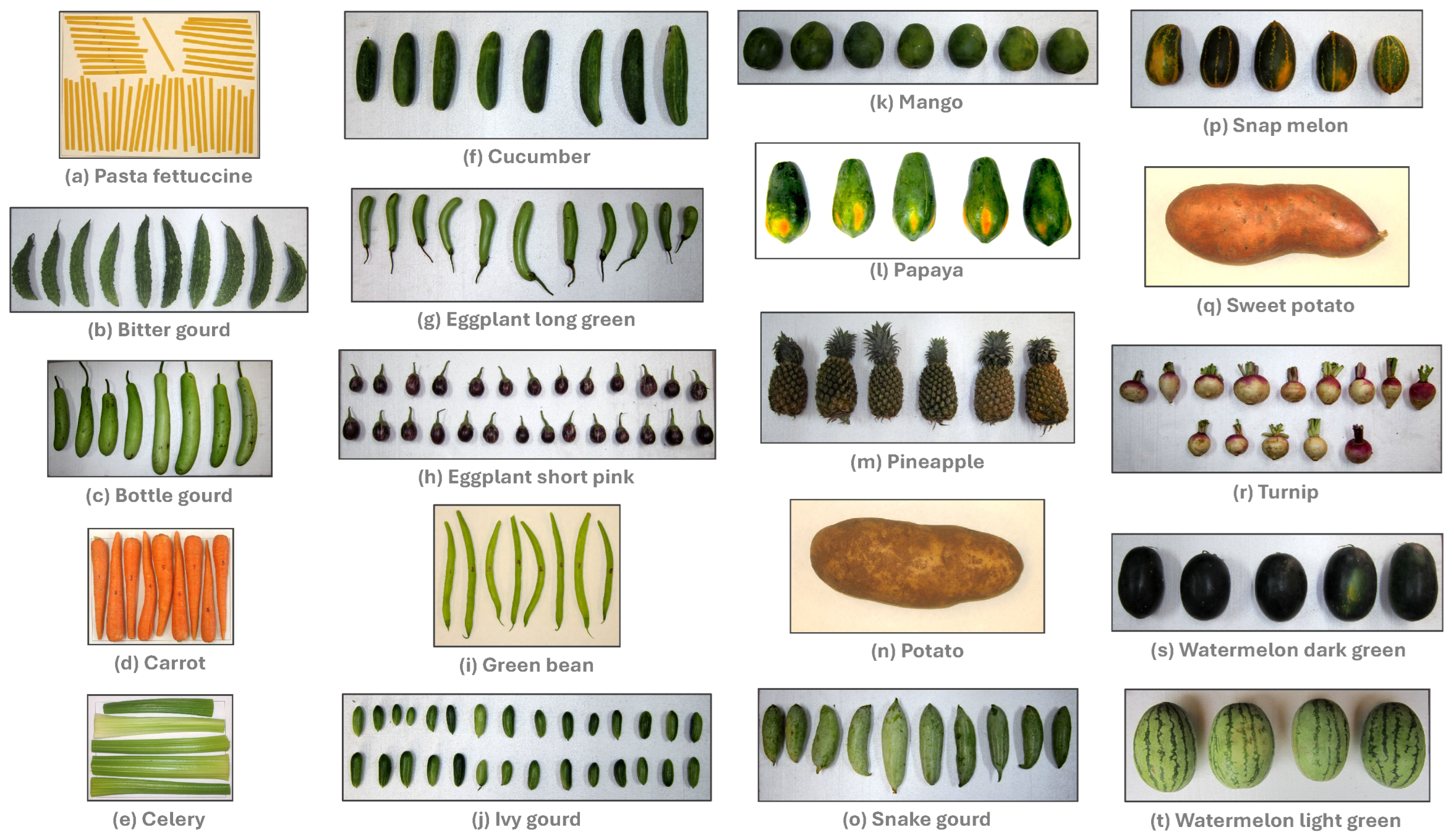
Figure 2.
Process flow diagram of multiple and mean dimensions of agricultural produce.
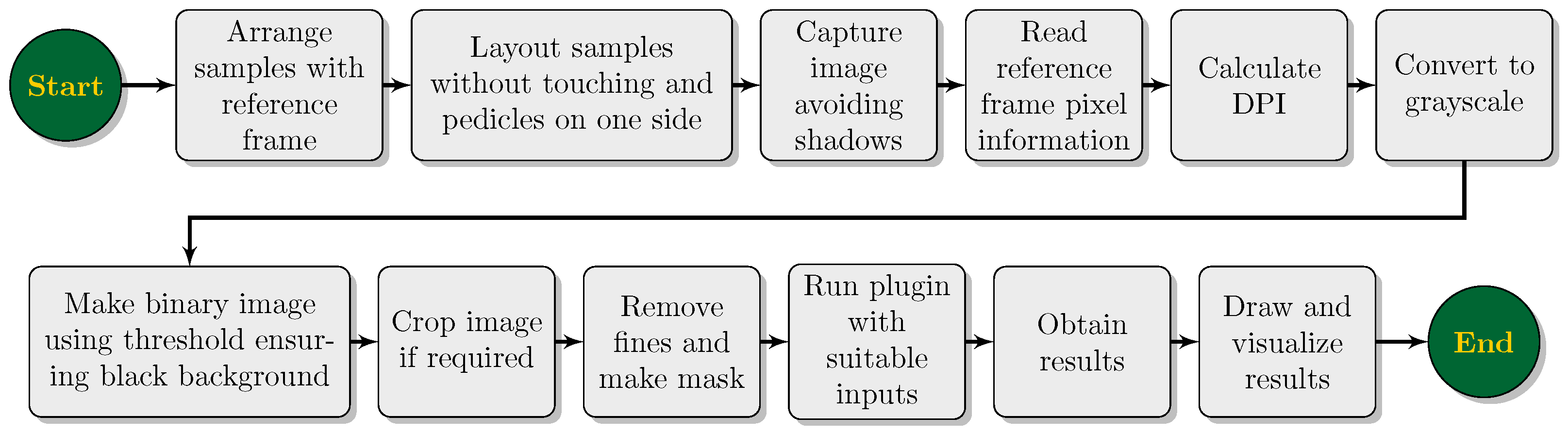
Figure 3.
Images captured using a digital camera with good contrast background and reference frame (left: snap melon on thermocol board - 1.0 0.5 ; right: celery on letter paper (US) with a drawn rectangle of 242 mm × 178 mm).
Figure 3.
Images captured using a digital camera with good contrast background and reference frame (left: snap melon on thermocol board - 1.0 0.5 ; right: celery on letter paper (US) with a drawn rectangle of 242 mm × 178 mm).
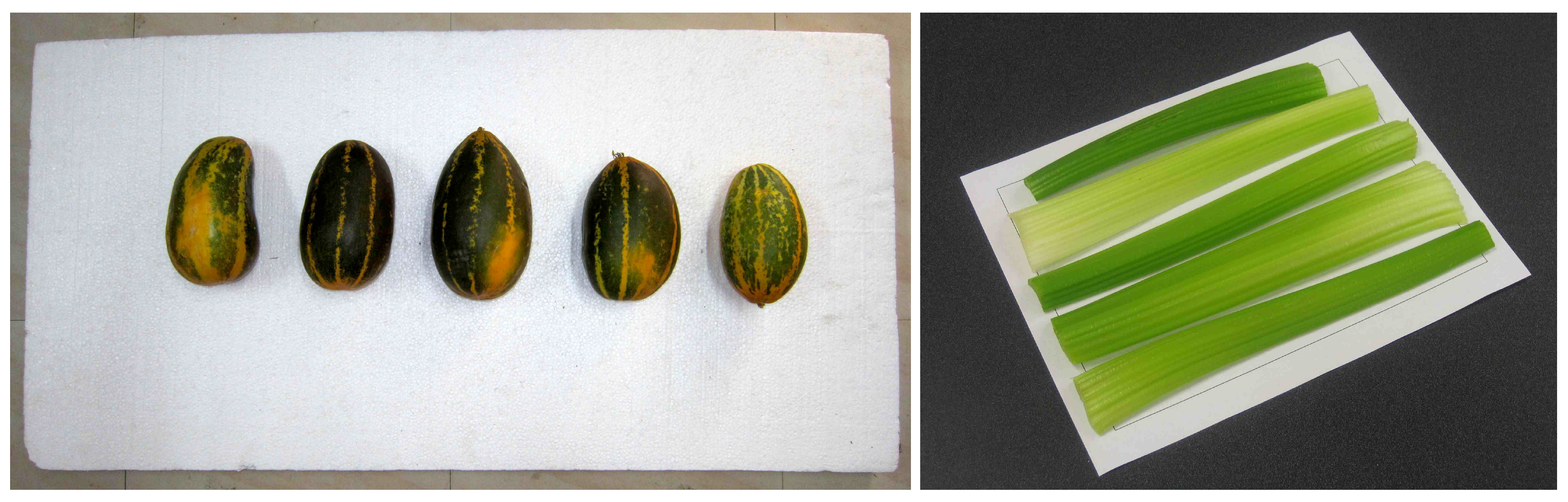
Figure 4.
Fiji environment and the developed plugin with its features. (A) Fiji ImageJ image processing software panel - where several standard tools and status bar are shown; (B) Standard “Analyze Particles” dialog box - which scans through various objects in the image and offers filtering options, such as fine particle removal, mask creation, excluding objects on edges, include holes in the object, and many more; (C) Developed plugin input panel - where calibration through DPI or reference frame dimensions, end caps chopping percentage, number of multiple widths measurement, and different output options can be input; (D) Measured multiple widths (50 numbers) from both edges of sample orthogonal to length from bottom to top; (E) multiple widths measurement drawing on a bottle gourd sample - where (1) centroid, (2) direction of length, (3) top cap chopped end, (4) bottom cap chopped end, (5) segment of measurement where multiple widths are measured, and (6) pedicle of the sample that was excluded using end cap values; (F) Standard ImageJ outputs of the object; (G) Section of textual output of individual width and their location along length; and (H) Consolidated numerical result of mean dimensions with standard deviation.
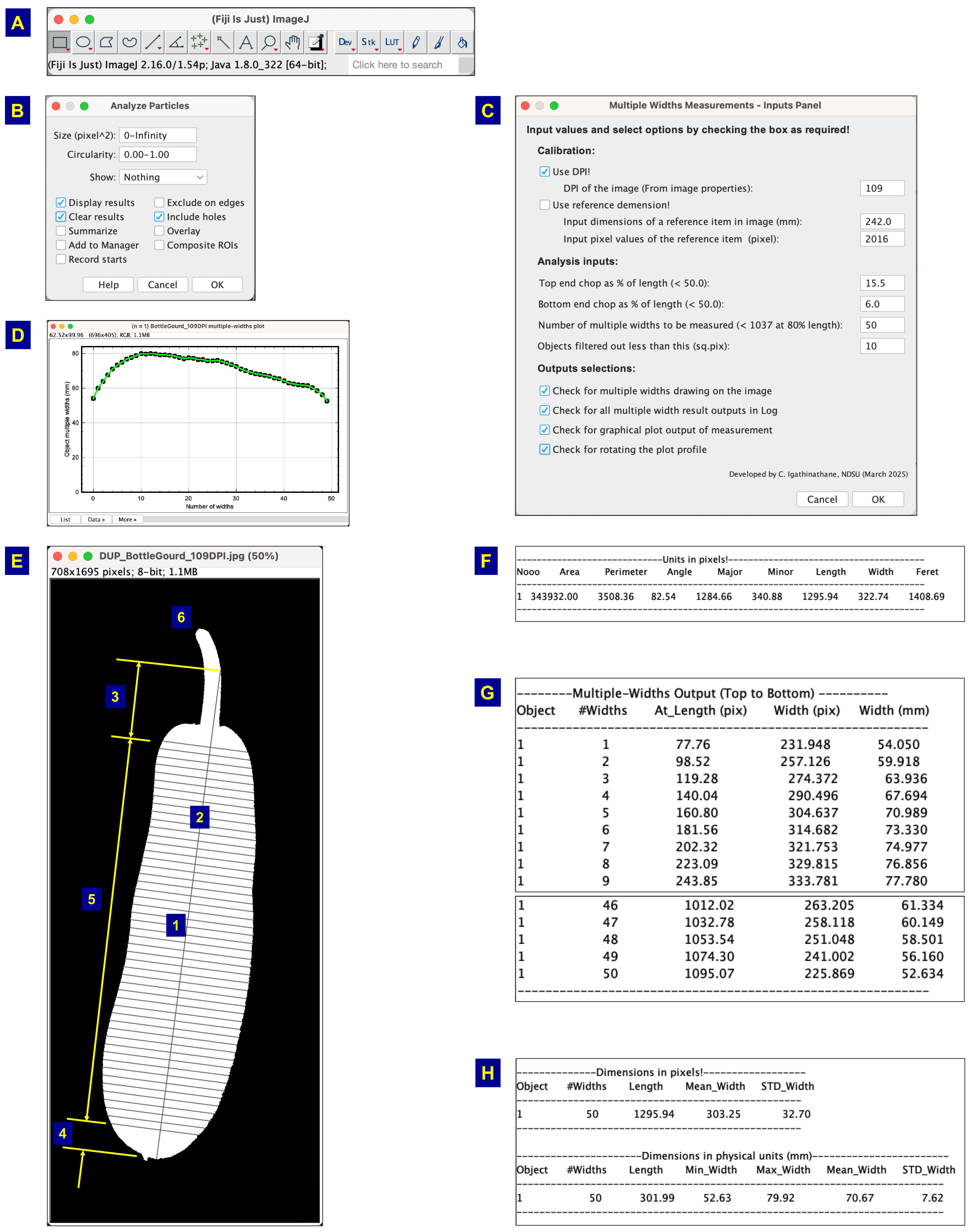
Figure 5.
Multiple width measurements validation using drawn rectangular blocks (1–4) and cut paper strips (5–10) of known dimensions (DPI = 256; 20 measurements; 10% end caps; labels indicate the object numbers).
Figure 5.
Multiple width measurements validation using drawn rectangular blocks (1–4) and cut paper strips (5–10) of known dimensions (DPI = 256; 20 measurements; 10% end caps; labels indicate the object numbers).
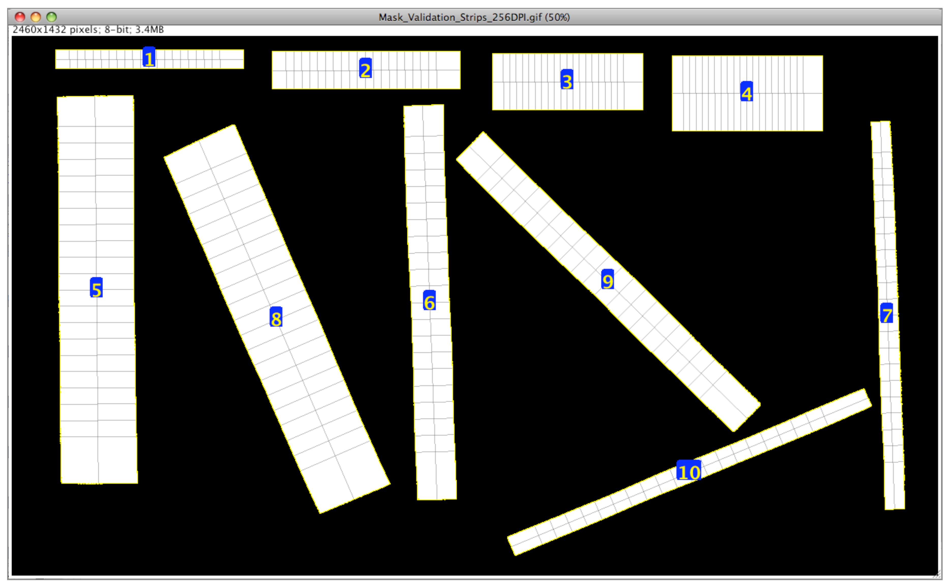
Figure 6.
Illustration of multiple width measurements using papaya sample image. (A) Original color image of the sample; (B) Binary mask of the original image used as plugin input where length and multiple widths were drawn, and (C) Multiple width plot for visualization of the measured widths and their profile.
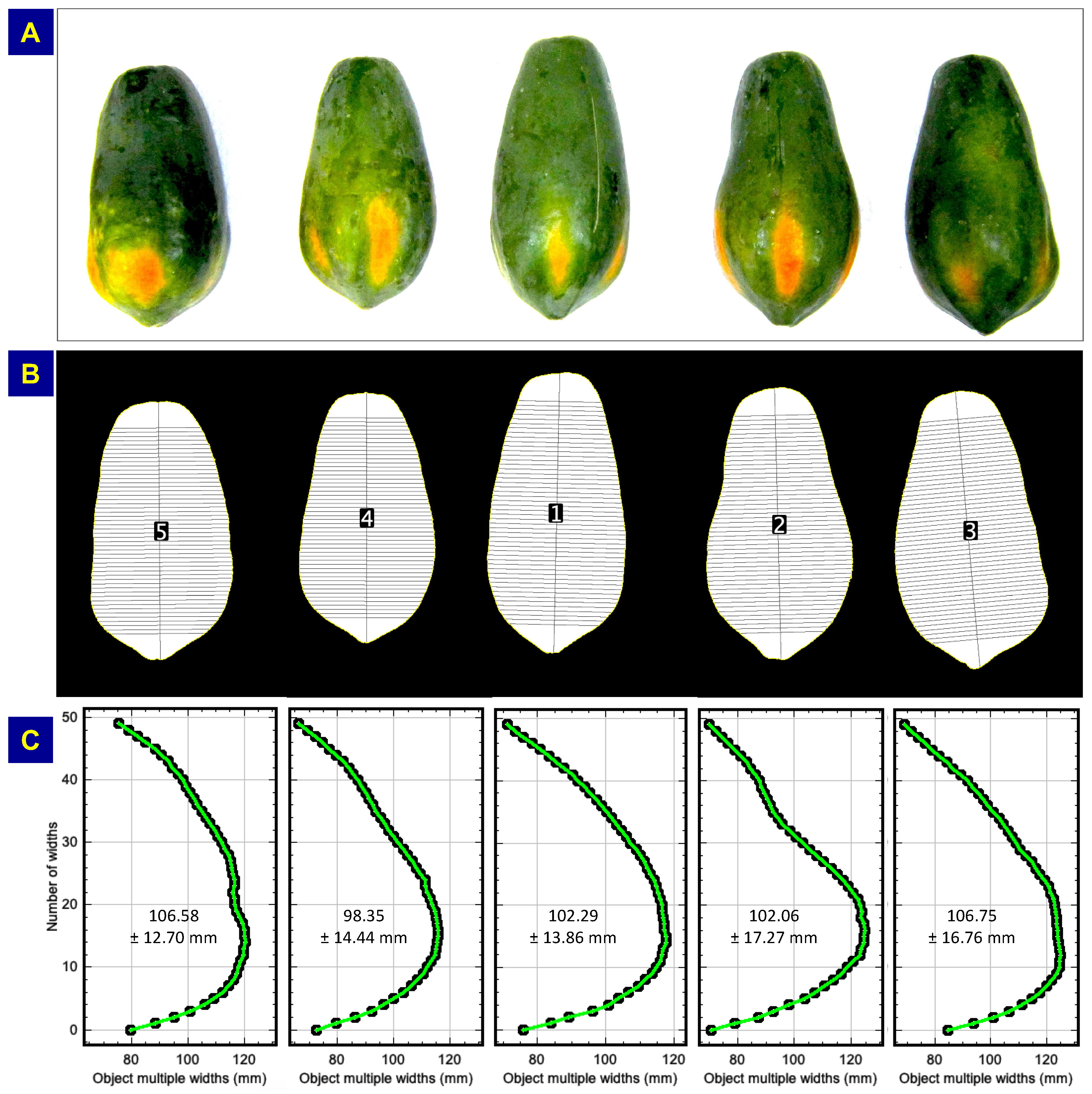
Figure 7.
Deviation of selected single and multiple widths from 50 multiple width measurements.
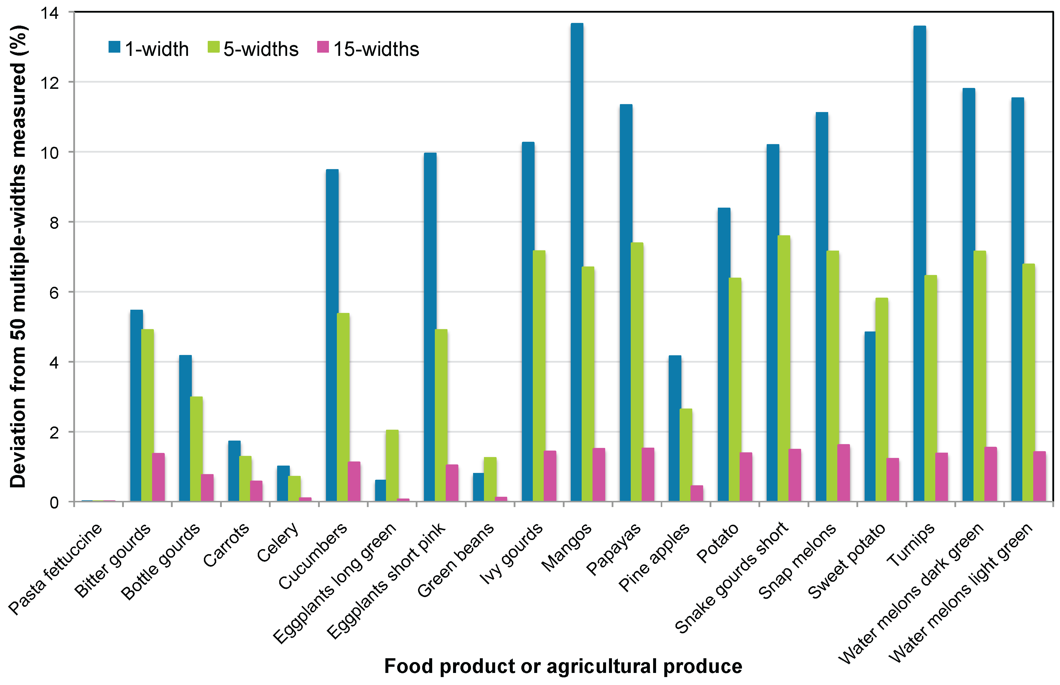

Table 1.
Validation results using drawn rectangular blocks, cut paper strips, and whole letter paper (US) of known dimensions (number of width measurements = 20).
Table 1.
Validation results using drawn rectangular blocks, cut paper strips, and whole letter paper (US) of known dimensions (number of width measurements = 20).
| Object | DPI | Actual (mm) | Plugin measured (mm) | Accuracy (%)# | ||||||
|---|---|---|---|---|---|---|---|---|---|---|
| length | width | length | width | length | width | |||||
| min | max | mean | STD | |||||||
| 256 | 500 | 50 | 500.00 | 50.010 | 50.010 | 50.01 | 0.00 | 100.00 | 99.98 | |
| 256 | 500 | 100 | 500.00 | 100.005 | 100.005 | 100 | 0.00 | 100.00 | 100.00 | |
| 256 | 400 | 150 | 400.00 | 150.003 | 150.003 | 150 | 0.00 | 100.00 | 100.00 | |
| 256 | 400 | 200 | 400.00 | 200.003 | 200.003 | 200 | 0.00 | 100.00 | 100.00 | |
| 256 | 100 | 20 | 102.50 | 19.74 | 20.04 | 19.85 | 0.09 | 97.50 | 99.25 | |
| 256 | 100 | 10 | 104.25 | 10.12 | 10.42 | 10.33 | 0.10 | 95.75 | 96.70 | |
| 256 | 100 | 5 | 102.36 | 4.96 | 5.46 | 5.21 | 0.11 | 97.64 | 95.80 | |
| 256 | 100 | 20 | 103.23 | 20.00 | 20.57 | 20.33 | 0.17 | 96.77 | 98.35 | |
| 256 | 100 | 10 | 102.79 | 10.31 | 10.59 | 10.43 | 0.10 | 97.21 | 95.70 | |
| 256 | 100 | 5 | 102.03 | 4.98 | 5.38 | 5.20 | 0.10 | 97.97 | 96.00 | |
| 165 | 279.4 | 108.9 | 278.66 | 107.61 | 109.46 | 108.50 | 0.56 | 99.74 | 99.63 | |
| 165 | 279.4 | 107.4 | 278.94 | 106.53 | 107.76 | 107.18 | 0.41 | 99.84 | 99.80 | |
| 165 | 279.4 | 215.9 | 278.84 | 214.17 | 216.33 | 215.19 | 0.67 | 99.80 | 99.67 | |
| 265 | 279.4 | 215.9 | 279.78 | 215.56 | 216.14 | 215.74 | 0.16 | 99.86 | 99.93 | |
Width columns min, max, and STD represent minimum, maximum, and standard deviation, respectively. * Blocks drawn using Fiji tools to exact pixel dimensions shown as actual length and widths (Figure 5); measurement resolution = 0.099 mm pixel−1. † Thin paper strips cut manually after drawing them (Figure 5); measurement resolution = 0.099 mm pixel−1. ‡ Two wider strips made by cutting a letter paper (US; 215.9 mm 279.4 mm) along the length (figure not shown); measurement resolution = 0.154 mm pixel−1. § Whole letter paper (US) is also included in the image of two wider strips (figure not shown); measurement resolution = 0.154 mm pixel−1. ¶ Whole letter paper (US) only with slightly increased DPI (figure not shown); measurement resolution = 0.096 mm pixel−1. # Accuracy (%) = [(Plugin measured - Actual)/Actual] × 100.
Table 2.
Results obtained from the plugin showing the measured dimensions of the agricultural produce (number of width measurements = 50).
Table 2.
Results obtained from the plugin showing the measured dimensions of the agricultural produce (number of width measurements = 50).
| N | Scientific name | #Objects | Plugin measured sample dimensions | † | ||||||
|---|---|---|---|---|---|---|---|---|---|---|
| Samples lengths (L, mm) | Samples widths (W, mm) | |||||||||
| Minimum | Maximum | Mean | Minimum | Maximum | Mean | |||||
| ± STD | ± STD | ± STD | ± STD | |||||||
| 1 | PastaFettuccine_252DPI | — | 48 | 69.95 | 99.04 | 85.10 ± 6.26 | 4.45 ± 0.03 | 4.98 ± 0.08 | 4.71 ± 0.05 | 0.06 |
| 2 | BitterGourds_109DPI | Momordica charatia | 10 | 159.64 | 290.62 | 237.24 ± 41.97 | 45.49 ± 3.87 | 58.06 ± 7.55 | 50.42 ± 5.58 | 0.22 |
| 3 | BottleGourds_109DPI | Lagenaria siceraria | 8 | 265.48 | 449.76 | 349.17 ± 61.44 | 60.41 ± 1.20 | 78.32 ± 12.11 | 67.47 ± 5.07 | 0.20 |
| 4 | Carrots_169DPI | Daucus carota | 9 | 179.76 | 210.27 | 196.98 ± 8.55 | 18.99 ± 3.51 | 28.80 ± 7.17 | 22.56 ± 5.92 | 0.11 |
| 5 | CeleryHearts_236DPI | Apium graveolensvar. Dulce | 5 | 206.97 | 263.76 | 247.11 ± 21.09 | 26.27 ± 1.49 | 41.21 ± 4.73 | 30.80 ± 2.89 | 0.12 |
| 6 | Cucumbers_109DPI | Cucumis sativus | 8 | 130.43 | 209.34 | 172.43 ± 23.09 | 40.05 ± 3.06 | 48.27 ± 4.99 | 43.79 ± 4.07 | 0.28 |
| 7 | EggplantLongGreen_109DPI | Solanum melongena | 11 | 96.94 | 198.4 | 151.30 ± 27.90 | 25.60 ± 2.65 | 35.26 ± 6.77 | 30.12 ± 4.54 | 0.20 |
| 8 | EggplantShortPink_109DPI | Solanum melongena | 27 | 62.89 | 96.07 | 75.25 ± 9.33 | 30.86 ± 2.75 | 45.42 ± 9.66 | 37.72 ± 4.29 | 0.55 |
| 9 | GreenBeans_244DPI | Phaseolus vulgaris | 7 | 79.36 | 123.09 | 104.79 ± 14.38 | 7.65 ± 0.15 | 10.33 ± 0.77 | 8.79 ± 0.34 | 0.08 |
| 10 | IvyGourds_109DPI | Coccinea indica | 29 | 39.89 | 74.6 | 60.79 ± 7.90 | 16.21 ± 2.08 | 25.15 ± 3.36 | 21.66 ± 2.72 | 0.39 |
| 11 | Mangos_109DPI | Mangifera indica | 7 | 114.7 | 132.57 | 121.79 ± 5.73 | 86.52 ± 11.10 | 101.15 ± 14.03 | 94.79 ± 12.35 | 0.88 |
| 12 | Papayas_109DPI | Carica papaya | 5 | 213.69 | 238.91 | 228.30 ± 9.74 | 98.35 ± 12.70 | 106.75 ± 17.27 | 103.21 ± 15.01 | 0.50 |
| 13 | Pineapple_109DPI | Ananas cosmosus | 6 | 234.67 | 276.97 | 260.26 ± 15.83 | 100.16 ± 4.24 | 121.59 ± 6.66 | 113.54 ± 5.05 | 0.45 |
| 14 | Potato_193DPI | Solanum tuberosum | 177.38 | 177.51 | 177.42 ± 0.06 | 64.80 ± 6.65 | 64.90 ± 6.92 | 64.86 ± 6.74 | 0.40 | |
| 15 | SnakeGourdsShort_109DPI | Trichosanthes cucumerina | 10 | 169.71 | 271.48 | 202.59 ± 31.52 | 50.14 ± 1.67 | 65.14 ± 12.28 | 57.18 ± 7.94 | 0.31 |
| 16 | SnapMelon_109DPI | Cucumis melovar. Momordica | 5 | 166.64 | 200.2 | 177.82 ± 11.95 | 90.09 ± 10.83 | 103.92 ± 16.47 | 98.87 ± 13.02 | 0.62 |
| 17 | SweetPotato_246DPI | Ipomoea batatas | 175.32 | 175.63 | 175.53 ± 0.15 | 60.19 ± 5.73 | 60.34 ± 6.09 | 60.28 ± 5.86 | 0.36 | |
| 18 | Turnips_109DPI | Brassica rapavar. Rapa | 14 | 95.5 | 150.35 | 117.67 ± 15.07 | 48.37 ± 6.98 | 99.14 ± 13.40 | 68.26 ± 10.28 | 0.66 |
| 19 | WaterMelonDarkGreen_109DPI | Citrulus lanatus | 5 | 201.52 | 232.1 | 214.87 ± 11.63 | 122.87 ± 14.23 | 143.46 ± 18.50 | 134.43 ± 16.07 | 0.70 |
| 20 | WaterMelonLightGreen_109DPI | Citrulus lanatus | 4 | 271.97 | 297.61 | 284.93 ± 9.12 | 171.94 ± 18.65 | 196.43 ± 24.00 | 187.28 ± 21.71 | 0.73 |
N - Number sequence. STD - Standard deviation obtained from the different objects of the sample from the same image representing a produce. * Image file name depicting the common name and the dots per inch (DPI) information of the captured image. † , width/length ratio (dimensionless), aka aspect ratio, width and length are the mean of single orthogonal measurements at the centroid of each sample. ‡ The three objects included are actually derived from the single original image by flipping it vertically and horizontally and combining them digitally.
Table 3.
Results obtained from the plugin showing the plugin measured dimensions of the agricultural produce (values presented are in mm, letters represent mean separation groups, and multiple-width measurements = 50).
Table 3.
Results obtained from the plugin showing the plugin measured dimensions of the agricultural produce (values presented are in mm, letters represent mean separation groups, and multiple-width measurements = 50).
| Pasta fettuccine | Bitter gourd | Bottle gourd | Carrot | Celery | Cucumber | Eggplant | |
|---|---|---|---|---|---|---|---|
| long green | |||||||
| 1 | 4.713 ± 0.00 A | 53.0 ± 0.05 A | 69.3 ± 0.10 C | 22.1 ± 0.02 B | 30.0 ± 0.03 A | 47.8 ± 0.02 B | 30.0 ± 0.04 B |
| 3 | 4.705 ± 0.00 A | 45.7 ± 0.04 B | 62.4 ± 0.10 A | 22.1 ± 0.02 B | 30.8 ± 0.03 A | 38.9 ± 0.02 D | 28.5 ± 0.03 A |
| 5 | 4.709 ± 0.00 A | 47.9 ± 0.05 E | 64.4 ± 0.10 AB | 22.2 ± 0.02 AB | 30.6 ± 0.03 A | 41.4 ± 0.02 E | 29.3 ± 0.04 AB |
| 7 | 4.706 ± 0.00 A | 48.6 ± 0.05 DE | 65.2 ± 0.10 AB | 22.3 ± 0.02 AB | 30.5 ± 0.03 A | 42.2 ± 0.02 C | 29.5 ± 0.04 B |
| 10 | 4.711 ± 0.00 A | 49.4 ± 0.05 CDE | 65.7 ± 0.10 ABC | 22.7 ± 0.02 A | 30.6 ± 0.03 A | 42.4 ± 0.02 C | 29.2 ± 0.04 AB |
| 15 | 4.708 ± 0.00 A | 49.7 ± 0.05 CD | 65.9 ± 0.10 ABC | 22.4 ± 0.02 AB | 30.4 ± 0.03 A | 43.2 ± 0.02 A | 29.8 ± 0.04 B |
| 20 | 4.710 ± 0.00 A | 50.1 ± 0.05 CD | 66.8 ± 0.10 BC | 22.6 ± 0.02 A | 30.4 ± 0.03 A | 43.3 ± 0.02 A | 29.6 ± 0.04 B |
| 25 | 4.711 ± 0.00 A | 50.1 ± 0.05 CD | 66.2 ± 0.10 BC | 22.4 ± 0.02 AB | 30.4 ± 0.03 A | 43.5 ± 0.02 A | 29.9 ± 0.04 B |
| 50 | 4.710 ± 0.00 A | 50.4 ± 0.05 C | 66.5 ± 0.10 BC | 22.5 ± 0.02 AB | 30.4 ± 0.03 A | 43.7 ± 0.02 A | 29.9 ± 0.04 B |
| 75 | 4.709 ± 0.00 A | 50.4 ± 0.05 C | 66.4 ± 0.10 BC | 22.4 ± 0.02 AB | 30.4 ± 0.03 A | 43.8 ± 0.02 A | 30.0 ± 0.04 B |
| 100 | 4.709 ± 0.00 A | 50.4 ± 0.05 C | 66.5 ± 0.10 BC | 22.5 ± 0.02 AB | 30.4 ± 0.03 A | 43.8 ± 0.02 A | 29.9 ± 0.04 B |
| 150 | 4.709 ± 0.00 A | 50.4 ± 0.05 C | 66.5 ± 0.10 BC | 22.5 ± 0.02 AB | 30.4 ± 0.03 A | 43.8 ± 0.02 A | 29.9 ± 0.04 B |
| 200 | 4.709 ± 0.00 A | 50.4 ± 0.05 C | 66.5 ± 0.10 BC | 22.4 ± 0.02 AB | 30.3 ± 0.03 A | 43.9 ± 0.02 A | 30.0 ± 0.04 B |
| #SigWidths ‡ | 1 ⇔ 1 | 50 ⇔ 7 | 20 ⇔ 3 | 10 ⇔ 3 | 1 ⇔ 1 | 15 ⇔ 10 | 7 ⇔ 3 |
| Eggplant | Green bean | Ivy gourd | Mango | Papaya | Pineapple | Potato | |
| short pink | |||||||
| 1 | 41.2 ± 0.02 F | 8.8 ± 0.01 B | 23.8 ± 0.01 C | 107.6 ± 0.01 G | 114.9 ± 0.03 G | 118.0 ± 0.03 D | 70.3 ± 0.01 J |
| 3 | 33.5 ± 0.01 G | 8.5 ± 0.01 A | 18.2 ± 0.01 F | 81.7 ± 0.02 F | 87.3 ± 0.02 F | 107.7 ± 0.03 E | 56.4 ± 0.01 I |
| 5 | 35.6 ± 0.01 D | 8.6 ± 0.01 AB | 20.0 ± 0.01 D | 88.4 ± 0.02 D | 95.5 ± 0.02 E | 110.3 ± 0.03 F | 60.7 ± 0.01 G |
| 7 | 36.3 ± 0.01 C | 8.7 ± 0.01 AB | 20.6 ± 0.01 B | 90.7 ± 0.02 C | 98.4 ± 0.03 D | 111.7 ± 0.03 CF | 62.3 ± 0.01 H |
| 10 | 36.5 ± 0.01 C | 8.7 ± 0.01 AB | 20.7 ± 0.01 B | 91.5 ± 0.02 C | 99.2 ± 0.03 D | 111.9 ± 0.03 BC | 62.9 ± 0.01 F |
| 15 | 37.1 ± 0.01 A | 8.7 ± 0.01 AB | 21.2 ± 0.01 E | 93.3 ± 0.02 E | 101.6 ± 0.03 C | 112.8 ± 0.03 ABC | 64.0 ± 0.01 E |
| 20 | 37.2 ± 0.01 AE | 8.7 ± 0.01 AB | 21.3 ± 0.01 E | 93.7 ± 0.02 E | 102.0 ± 0.03 BC | 112.7 ± 0.03 ABC | 64.2 ± 0.01 D |
| 25 | 37.4 ± 0.01 AB | 8.7 ± 0.01 B | 21.4 ± 0.01 AE | 94.1 ± 0.02 AE | 102.5 ± 0.03 ABC | 113.0 ± 0.03 ABC | 64.5 ± 0.01 C |
| 50 | 37.5 ± 0.01 AB | 8.7 ± 0.01 B | 21.5 ± 0.01 A | 94.7 ± 0.02 AB | 103.1 ± 0.03 AB | 113.3 ± 0.03 AB | 64.9 ± 0.01 A |
| 75 | 37.6 ± 0.01 BE | 8.8 ± 0.01 B | 21.6 ± 0.01 A | 94.9 ± 0.02 AB | 103.4 ± 0.03 A | 113.4 ± 0.03 AB | 65.0 ± 0.01 AB |
| 100 | 37.6 ± 0.01 BE | 8.8 ± 0.01 B | 21.6 ± 0.01 A | 95.0 ± 0.02 AB | 103.4 ± 0.03 A | 113.4 ± 0.03 AB | 65.0 ± 0.01 AB |
| 150 | 37.6 ± 0.01 B | 8.8 ± 0.01 B | 21.6 ± 0.01 A | 95.1 ± 0.02 B | 103.5 ± 0.03 A | 113.4 ± 0.03 A | 65.1 ± 0.01 B |
| 200 | 37.6 ± 0.01 B | 8.8 ± 0.01 B | 21.6 ± 0.01 A | 95.1 ± 0.02 B | 103.6 ± 0.03 A | 113.5 ± 0.03 A | 65.1 ± 0.01 B |
| #SigWidths ‡ | 75 ⇔ 15 | 25 ⇔ 3 | 50 ⇔ 20 | 50 ⇔ 20 | 75 ⇔ 20 | 150 ⇔ 10 | 150 ⇔ 50 |
| Snake gourd | Snap melon | Sweet potato | Turnip | Watermelon | Watermelon | ||
| dark green | light green | ||||||
| 1 | 62.7 ± 0.06 D | 109.8 ± 0.06 F | 63.2 ± 0.01 A | 76.6 ± 0.05 F | 150.1 ± 0.03 A | 208.5 ± 0.04 F | |
| 3 | 47.7 ± 0.05 C | 83.9 ± 0.05 E | 52.7 ± 0.01 H | 57.3 ± 0.05 E | 114.4 ± 0.03 G | 160.6 ± 0.03 C | |
| 5 | 52.6 ± 0.05 A | 91.8 ± 0.06 D | 56.8 ± 0.01 G | 62.5 ± 0.05 C | 124.7 ± 0.03 F | 174.4 ± 0.03 A | |
| 7 | 54.2 ± 0.05 AB | 94.3 ± 0.06 CD | 58.1 ± 0.01 F | 64.2 ± 0.05 BC | 128.3 ± 0.03 E | 179.2 ± 0.03 G | |
| 10 | 54.7 ± 0.05 BE | 95.9 ± 0.06 BC | 58.4 ± 0.01 E | 64.9 ± 0.05 BD | 129.3 ± 0.03 E | 180.6 ± 0.03 G | |
| 15 | 56.1 ± 0.05 EF | 97.2 ± 0.06 AB | 59.6 ± 0.01 D | 66.1 ± 0.05 AB | 132.2 ± 0.03 D | 184.4 ± 0.04 E | |
| 20 | 56.2 ± 0.05 EF | 98.0 ± 0.06 AB | 59.7 ± 0.01 D | 66.3 ± 0.05 AD | 132.7 ± 0.03 CD | 185.1 ± 0.04 DE | |
| 25 | 56.6 ± 0.05 EF | 98.1 ± 0.06 AB | 60.0 ± 0.01 C | 67.7 ± 0.04 A | 133.4 ± 0.03 BCD | 185.9 ± 0.04 BDE | |
| 50 | 57.0 ± 0.05 F | 98.8 ± 0.06 A | 60.3 ± 0.01 B | 67.1 ± 0.05 A | 134.2 ± 0.03 BC | 187.0 ± 0.04 BD | |
| 75 | 57.1 ± 0.05 F | 98.9 ± 0.06 A | 60.4 ± 0.01 B | 67.2 ± 0.05 A | 134.5 ± 0.03 B | 187.4 ± 0.04 BD | |
| 100 | 57.1 ± 0.05 F | 99.1 ± 0.06 A | 60.4 ± 0.01 B | 67.3 ± 0.05 A | 134.7 ± 0.03 B | 187.6 ± 0.04 B | |
| 150 | 57.2 ± 0.05 F | 99.2 ± 0.06 A | 60.5 ± 0.01 B | 67.4 ± 0.05 A | 134.8 ± 0.03 B | 187.8 ± 0.04 B | |
| 200 | 57.2 ± 0.05 F | 99.2 ± 0.06 A | 60.5 ± 0.01 B | 67.4 ± 0.05 A | 134.9 ± 0.03 B | 187.9 ± 0.04 B | |
| #SigWidths ‡ | 50 ⇔ 10 | 50 ⇔ 10 | 50 ⇔ 25 | 25 ⇔ 10 | 75 ⇔ 20 | 100 ⇔ 20 |
† Number of multiple width measurements considered. Values shown are estimated mean ± standard error estimate in mm; uppercase letter grouping having a common letter(s) indicates that the means are not significantly different ( = 0.05). ‡ Maximum number of significant multiple widths shown in the form: a⇔b; where, a represents the minimum number of multiple width measurements above which means are not significantly different ( = 0.05); and b is the next below significantly different multiple widths of b.
Disclaimer/Publisher’s Note: The statements, opinions and data contained in all publications are solely those of the individual author(s) and contributor(s) and not of MDPI and/or the editor(s). MDPI and/or the editor(s) disclaim responsibility for any injury to people or property resulting from any ideas, methods, instructions or products referred to in the content. |
© 2025 by the authors. Licensee MDPI, Basel, Switzerland. This article is an open access article distributed under the terms and conditions of the Creative Commons Attribution (CC BY) license (http://creativecommons.org/licenses/by/4.0/).
Copyright: This open access article is published under a Creative Commons CC BY 4.0 license, which permit the free download, distribution, and reuse, provided that the author and preprint are cited in any reuse.


