
Submitted:
01 June 2025
Posted:
03 June 2025
You are already at the latest version
Abstract
Accurate estimation of soil properties is crucial for optimizing agricultural practices and promoting sustainable resource management. Hyperspectral imaging provides a non-invasive means of quantifying key soil parameters, but effectively utilizing the high-dimensional hyperspectral data presents significant challenges. In this paper, we introduce HyperSoilNet, a hybrid deep learning framework for estimating soil properties from hyperspectral imagery. HyperSoilNet leverages a pretrained hyperspectral-native CNN backbone and integrates it with a carefully optimized machine learning (ML) ensemble to combine the strengths of deep representation learning with traditional ML techniques. We evaluate our framework on the Hyperview challenge dataset, focusing on four critical soil properties: potassium, phosphorus pentoxide, magnesium, and soil pH. Comprehensive experiments demonstrate that HyperSoilNet surpasses state-of-the-art models, achieving a score of 0.762 on the challenge leaderboard. Through detailed ablation studies and spectral analysis, we provide insights on the components of the framework, and their contribution to performance, showcasing its potential for advancing precision agriculture and sustainable soil management practices.
Keywords:
hyperspectral imaging
; soil property estimation
; self-supervised learning
; deep learning
; remote sensing
; precision agriculture
1. Introduction
The rising global food demand and increasing environmental concerns have made monitoring soil health a critical priority for sustainable agriculture [1]. Precision agriculture, which involves tailoring agricultural inputs to site-specific conditions, has emerged as a promising approach to improve crop yields while minimizing negative environmental impacts [2]. Accurate estimation of soil properties, such as nutrient levels and pH, is central to precision agriculture, as these properties directly influence crop growth, soil health, and the effectiveness of agricultural interventions [3].
Traditional methods for assessing soil properties rely on physical sampling and laboratory analysis. While these methods are reliable, they are labor-intensive, costly, and they provide only point-based measurements that may not represent larger field variability [4]. Such sparse and localized sampling can miss important spatial patterns of soil nutrients or contaminants. Remote sensing techniques have therefore gained traction as a complementary, non-invasive approach to soil analysis [4,5,6].
Hyperspectral imaging (HSI) captures reflectance data across hundreds of narrow, contiguous spectral bands, providing means to assess soil characteristics over broad areas without direct contact with the ground [7,8]. Each soil property (such as organic matter, moisture, or mineral content) imparts subtle but detectable features in the soil’s spectral signature. By measuring reflectance across a wide spectrum, HSI can differentiate materials based on their unique spectral signature, enabling the detection of variations in soil composition and condition [9]. This capability makes HSI an indispensable tool for mapping soil properties over large agricultural regions in a rapid and cost-effective manner.
Despite its potential, hyperspectral data poses significant challenges due to its high dimensionality and complexity. A single HSI scene can have hundreds of bands, resulting in a large feature space from which relevant spectral-spatial patterns are difficult to extract. Traditional machine learning methods frequently struggle with these high-dimensional data and the nonlinear relationships between spectral features and soil properties [10,11]. Simpler models may fail to capture the variety of spectral signatures associated with different soil parameters, particularly under changing field conditions (e.g., moisture or surface residue changes). This complexity demands more advanced analytical techniques capable of extracting meaningful information from HSI while avoiding overfitting and noise sensitivity.
Deep learning (DL) approaches, particularly convolutional neural networks (CNNs), have shown considerable success in various computer vision tasks, including hyperspectral image analysis [12,13,14,15,16]. Specialised deep models have achieved state-of-the-art performance in tasks such as hyperspectral image classification and segmentation [17]. However, most existing DL models for hyperspectral regression require a large amount of labeled training data to learn effectively. Labeled data in agricultural applications (for example, ground-truth soil measurements coincident with HSI) is frequently limited, expensive to obtain, and does not usually cover all conditions. As a result, purely deep models are prone to overfitting on small datasets and may perform poorly when applied to new regions or soil types [18,19]. Recent advances in self-supervised learning offer a promising avenue to tackle the data scarcity problem. By pulling together (in feature space) different augmented views of the same sample and pushing apart views of different samples, contrastive frameworks enable models to capture spectral patterns without relying on extensive labeled datasets [20]. Such techniques have produced impressive results in both general computer vision and remote sensing applications [21,22], indicating the possibility of improving feature extraction for hyperspectral data. Pretraining a model in a self-supervised manner on a large collection of HSI (without the need for ground-truth labels) allows one to initialise the model with more robust and informative spectral feature encodings for downstream regression tasks.
Another promising approach to improving soil property prediction is through the development of hybrid frameworks that combine the strengths of deep learning and classical machine learning. In this hybrid approach, a deep neural network can act as a feature extractor, distilling the high-dimensional hyperspectral data into a compact set of informative features, while traditional machine learning models (or ensembles) can be used as final predictors for soil parameters. By combining deep and shallow learners, one can achieve a form of regularisation. The deep model transforms the input into a lower-dimensional feature space, while the downstream ML model reduces overfitting through ensemble averaging and other constraints. This synergy is especially useful in scenarios with limited training data.
In this paper, we introduce HyperSoilNet, a hybrid framework for soil property estimation from hyperspectral imagery. HyperSoilNet integrates a hyperspectral-native CNN backbone with a self-supervised contrastive learning scheme and a machine learning ensemble for regression. We apply HyperSoilNet to the HyperView Challenge dataset [23], a recent benchmark for soil property prediction from satellite-based HSI focusing on four important soil parameters: potassium (K), phosphorus pentoxide , magnesium (Mg), and pH. Our experimental results show that the proposed approach outperforms existing state-of-the-art models on this dataset, highlighting its potential for advancing precision agriculture and sustainable soil management.
In summary, our contributions are: (1) We propose a hybrid framework (HyperSoilNet) that integrates a hyperspectral CNN backbone and an ensemble of traditional ML regressors to estimate soil properties. (2) We demonstrate the effectiveness of this approach on a public benchmark dataset. (3) We provide an analysis of the framework’s components. The remainder of this paper is organized as follows: Section 2 reviews relevant literature for soil property estimation using hyperspectral data. Section 3 details the proposed hybrid methodology. Section 4 presents the experimental setup and results, and Section 5 presents a discussion of the results and insights into the model’s performance. Finally, Section 6 concludes the paper with a summary and suggestions for future work.
2. Related Work
Hyperspectral Imaging for Soil Analysis: Hyperspectral remote sensing has a rich history in soil and agricultural applications, providing a means to assess soil properties across large areas with high spectral fidelity. HSI enables the identification of soil constituents such as minerals, organic matter, moisture, and nutrients based on their spectral signatures [24]. Numerous studies have leveraged hyperspectral data for in situ soil property estimation, often in the context of precision agriculture and land management. Early approaches drew from techniques in spectroscopy and chemometrics, using statistical analysis of spectra or handcrafted spectral indices to infer soil parameters. For example, vegetation and soil indices (like NDVI and its soil-adjusted variants) have been employed to indirectly estimate properties like soil organic carbon or fertility [25]. More specifically, partial least squares regression (PLSR) and other multivariate regression methods have traditionally been used to model the relationship between lab-measured soil properties and their spectral reflectance, particularly in studies involving soil spectral libraries or field spectrometer data [26,27]. These traditional methods were effective in many cases, establishing a baseline performance for soil prediction tasks. However, as the availability of hyperspectral imagery has grown, so has the need to map soil properties at scale, introducing greater variability in soil conditions and imaging factors. To address this complexity, the community has gradually incorporated more powerful machine learning techniques than linear regression.
Classical Machine Learning Approaches: A variety of traditional machine learning (ML) models have been used to predict soil properties from spectral data. Support vector machines (SVMs) and random forest (RF) ensembles are popular choices that have demonstrated strong performance in numerous case studies [28]. These models can capture nonlinear relationships between spectral features and soil properties and tend to be more robust than simple linear models. For instance, Abdulraheem et al. [4] provide a comprehensive review of remote sensing methods for soil measurement, highlighting the effectiveness of tree-based ensembles and kernel methods in this domain. In many studies, a common workflow is to first perform feature extraction or selection on the hyperspectral data (for example, using principal components, band selection, or expert-designed spectral features) and then train an ML regressor on those features [29,30]. While these traditional approaches can achieve good performance, particularly when calibrated to a specific region or dataset, they may struggle to generalise broadly. One significant limitation is that manually crafted features or shallow decision boundaries may not fully capture the complex, high-order interactions found in full-spectrum hyperspectral data.
Deep Learning Methods: Deep learning has increasingly been explored for modeling hyperspectral data, including soil parameter estimation. Deep neural networks can automatically learn feature representations from raw spectral images, potentially uncovering subtler patterns than manual feature engineering. For example, Zhong et al. [31] demonstrated that a deep CNN outperformed a shallow CNN and traditional ML methods for predicting soil properties in the large LUCAS soil dataset. Other architectures such as autoencoders and recurrent neural networks (RNNs) have also been investigated. Autoencoders (stacked denoising autoencoders, in particular) have been used to learn unsupervised spectral features that improve subsequent prediction of multiple soil attributes [32,33]. More recently, attention mechanisms and transformer-based architectures have been introduced to hyperspectral analysis [34,35]. Overall, deep learning methods have pushed the performance boundaries in soil spectroscopy, but they often require careful regularization, large training datasets, or transfer learning to be effective, due to the risk of overfitting in data-scarce scenarios [18,19].
Hybrid and Ensemble Frameworks: An emerging trend in the field is the development of hybrid frameworks that seek to harness the complementary advantages of different approaches. Rather than viewing classical ML and deep learning as mutually exclusive solutions, recent research shows that combining them can lead to more robust and generalized models [36,37,38]. Another approach is the model ensembling of heterogeneous learners. For example, ensemble models that combine the outputs of neural networks and traditional ML models can often outperform either model alone, by reducing variance and exploiting different modeling strengths. The benefits of such hybrid strategies were evident in the 2022 HyperView Challenge (a competition for predicting soil properties from hyperspectral images). The Hyperview Challenge winner, EagleEyes [39], combined random forest and KNN with hand-crafted features, achieving a score of 0.781. However, its reliance on manual feature engineering limits scalability. HyperSoilNet advances this paradigm by integrating a self-supervised Hyperspectral CNN backbone with an ML ensemble, leveraging unlabeled data to automate feature extraction while maintaining prediction accuracy.
Research Gaps and Motivation: Despite the progress in applying traditional ML and DL to hyperspectral soil data, there remain noteworthy gaps in the literature. Many studies either rely solely on classical ML or on end-to-end deep networks; relatively few attempts have been made to integrate these approaches into a cohesive framework for regression tasks. The potential of self-supervised learning in this domain is also largely untapped. Most prior works train on labeled data only, overlooking the value of abundant unlabeled hyperspectral data to pretrain models. While recent reviews highlight self-supervised learning as a rising trend in remote sensing [21], applications in soil property prediction are still in their early stages. Our work is motivated to develop a hybrid approach that combines self-supervised feature learning and ensemble modelling to improve generalisation. To our knowledge, this is the first approach to integrate contrastive self-supervised learning with a classical ML ensemble for hyperspectral soil property estimation. In the following sections, we build upon the insights from prior work and detail how our method is designed to advance the state of the art in non-invasive soil property estimation.
Figure 1.
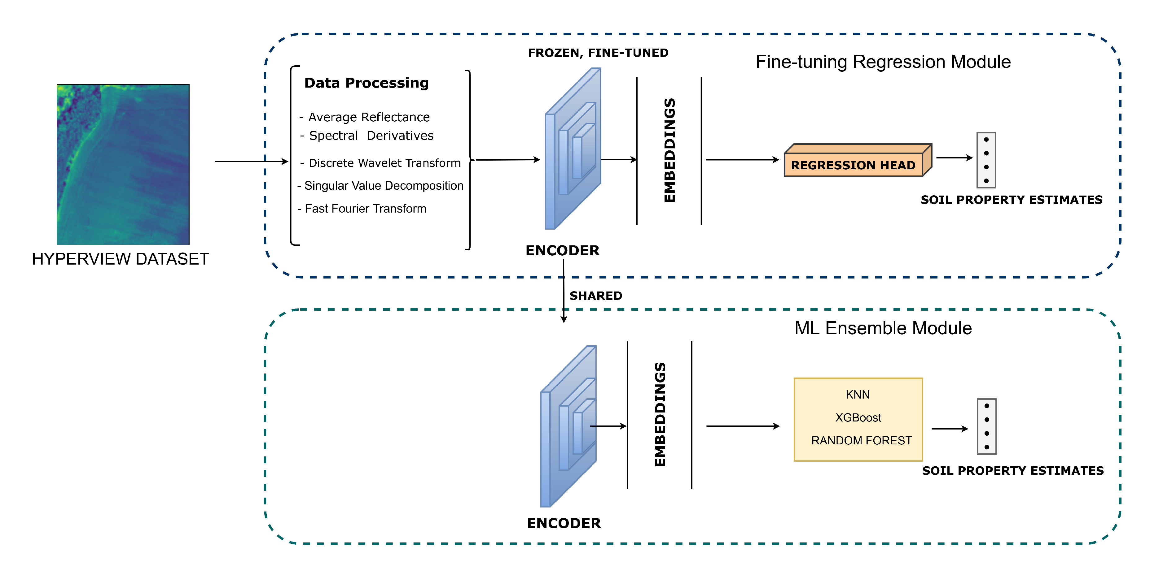
Architecture of the proposed HyperSoilNet framework. The framework consists of two main phases: (1) A Fine-tuning Regression Module (top) that leverages the pretrained encoder (frozen weights) along with comprehensive feature engineering techniques (average reflectance, spectral derivatives, discrete wavelet transform, SVD, and FFT) to extract informative representations for soil property estimation; and (2) An ML Ensemble Module (bottom) that utilizes the shared embeddings to feed a combination of ML regressors for soil property prediction. The arrows indicate the flow of information between modules, with the pretrained encoder being adapted for the downstream soil estimation task.
Figure 1.
Architecture of the proposed HyperSoilNet framework. The framework consists of two main phases: (1) A Fine-tuning Regression Module (top) that leverages the pretrained encoder (frozen weights) along with comprehensive feature engineering techniques (average reflectance, spectral derivatives, discrete wavelet transform, SVD, and FFT) to extract informative representations for soil property estimation; and (2) An ML Ensemble Module (bottom) that utilizes the shared embeddings to feed a combination of ML regressors for soil property prediction. The arrows indicate the flow of information between modules, with the pretrained encoder being adapted for the downstream soil estimation task.
3. Methodology
In this work, we present a hybrid framework for soil property estimation from hyperspectral imagery called HyperSoilNet. Our approach integrates a pretrained deep learning backbone with traditional machine learning regressors to effectively leverage both representation learning and ensemble prediction. The entire workflow is designed to address the challenges of high-dimensional hyperspectral data while maximizing prediction accuracy for soil properties.
3.1. Dataset Characteristics and Analysis
The experiments in this study were conducted using the Hyperview dataset, a collection of high-quality hyperspectral imagery and corresponding ground truth soil measurements, provided as part of the Hyperview Challenge organized by KP Labs, ESA, and QZ Solutions [23]. Before describing our methodology, we first analyze key characteristics of this dataset that influenced our approach.
The dataset was acquired over Polish agricultural areas in March 2021 using a HySpex VS-725 hyperspectral imager mounted on a Piper PA-31 Navajo aircraft. This imaging system comprises SWIR-384 and VNIR-1800 imagers, capturing a total of 430 hyperspectral bands, which were subsequently reduced to 150 bands to match the spectral range of the Intuition-1 satellite’s onboard sensor. Ground truth measurements of soil properties were obtained through in-situ sampling and analysis using the Mehlich 3 methodology [40,41]. The dataset consists of 2886 patches (1732 for training and 1154 for testing), with each patch containing 150 spectral bands and representing a field with four ground truth soil parameters.
Figure 2.
Representative spectral signatures from the Hyperview dataset. (a) Mean spectral reflectance curves for fields with different potassium (K) levels. (b) Mean spectral reflectance curves for fields with different phosphorus pentoxide (P2O5) levels. (c) Mean spectral reflectance curves for fields with different magnesium (Mg) levels. (d) Mean spectral reflectance curves for fields with different pH levels. Shaded regions represent one standard deviation around the mean.
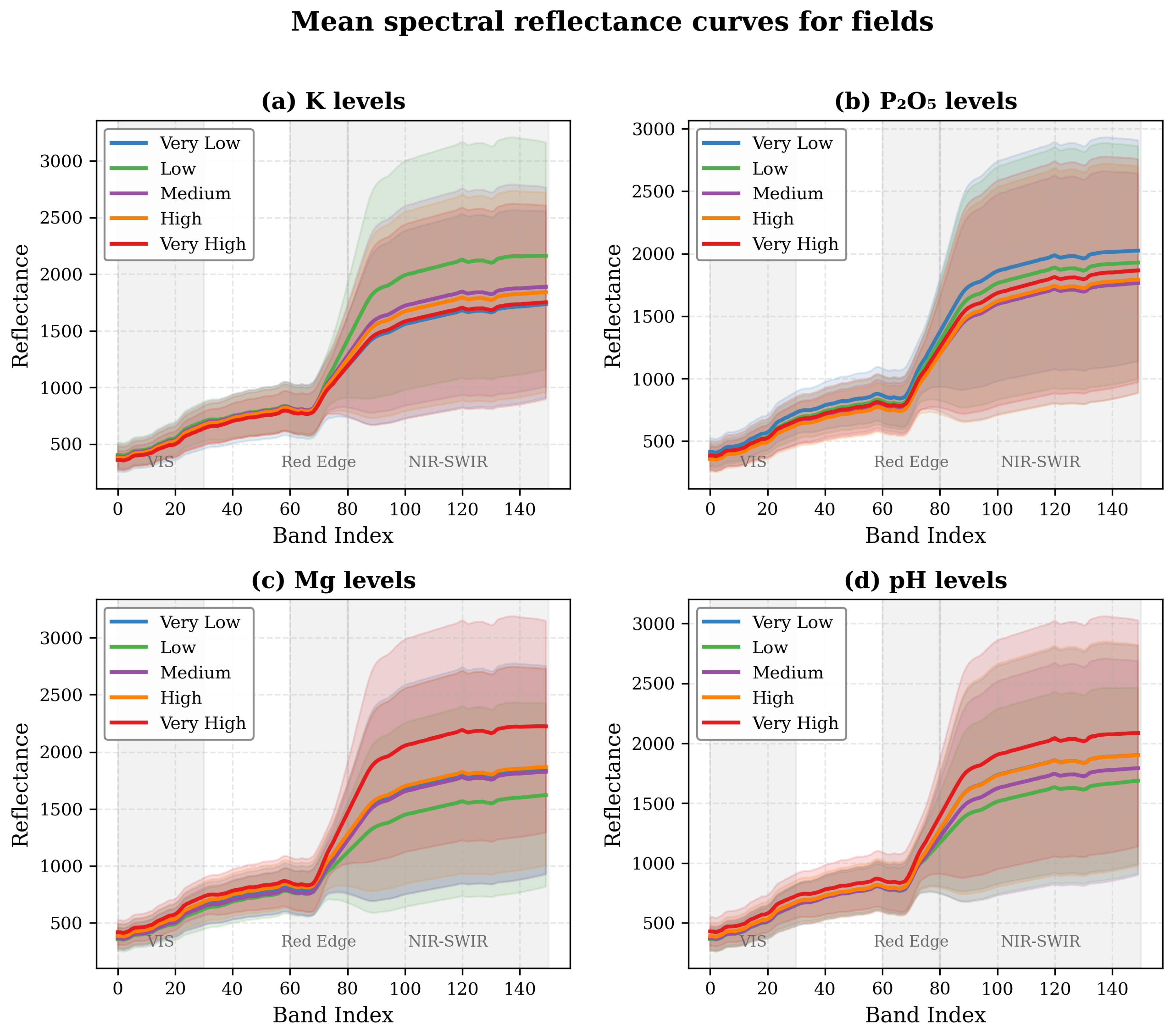
Examination of the spectral signatures for fields with varying soil properties reveals subtle but distinctive patterns (Figure 2). The spectral differences between soil parameter levels are most pronounced in the NIR-SWIR region (bands 80-150), with a distinctive reflectance increase after the Red Edge region (bands 60-80). In particular, fields with high Mg and pH levels show notably higher reflectance in the NIR-SWIR region compared to those with lower values, while K and P2O5 differences are more subtle. This aligns with known absorption features of soil minerals and organic matter, providing a physical basis for spectral discrimination.
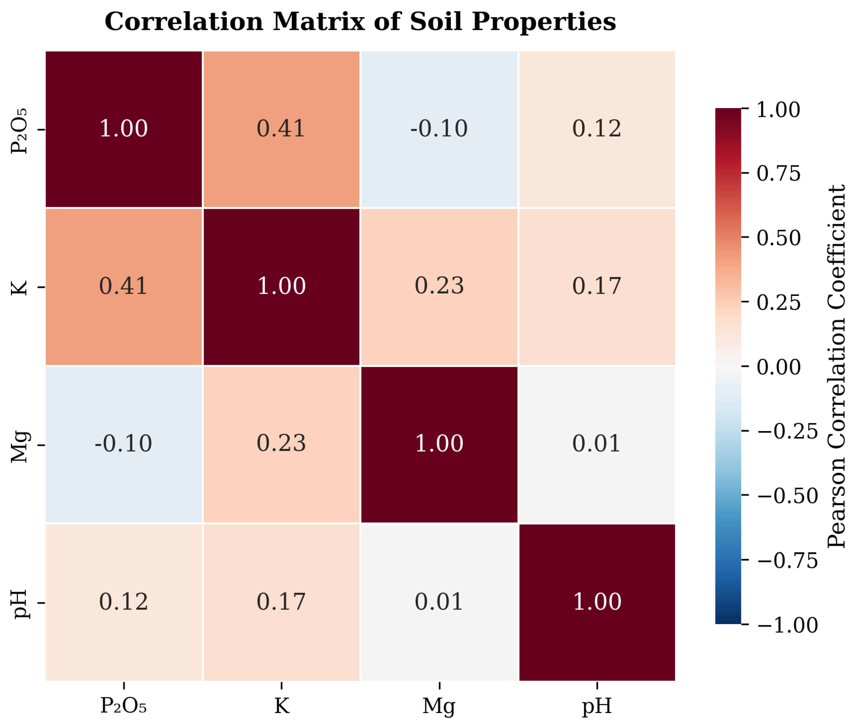
The distribution of soil properties across the training dataset exhibits notable patterns, with K, P2O5, and Mg showing right-skewed distributions (most fields having lower to medium values), while pH follows a more normal distribution centered around 6.8. Correlation analysis between soil properties (Figure 3) revealed a moderate positive correlation between K and P2O5 (r = 0.41), suggesting these macronutrients share common dynamics in the studied soils. K and Mg showed a weaker positive relationship (r = 0.23), while a slight negative correlation exists between P2O5 and Mg (r = -0.10). The correlations between pH and other properties were particularly weak (r = 0.01 to 0.17), confirming that soil acidity is largely independent of nutrient content in this dataset.
These observations guided our feature engineering process and model design choices, highlighting the need for techniques that can capture the subtle spectral variations in the VIS (bands 0-30) and Red Edge regions, while leveraging the more prominent differences in the NIR-SWIR bands. The varying correlation strengths between soil properties further supported our multi-task learning approach, which can leverage shared information for correlated properties while maintaining specificity for more independent variables like pH.
Figure 3.
Correlation matrix of soil properties in the Hyperview training dataset. Color intensity and numbers represent Pearson correlation coefficients.
Figure 3.
Correlation matrix of soil properties in the Hyperview training dataset. Color intensity and numbers represent Pearson correlation coefficients.
3.2. Framework Overview
HyperSoilNet consists of two main components, as illustrated in Figure 1. The foundation of the first component is a pretrained Hyperspectral-Native CNN Backbone based on the HyperKon architecture [42], which was previously trained on a large collection of hyperspectral satellite imagery using contrastive learning. This backbone serves as our feature extractor, providing robust spectral-spatial representations that have been learned from diverse hyperspectral data. Then we adapt the pretrained backbone for soil property estimation. The second component is an ML Ensemble Module which employs multiple traditional machine learning regressors that operate on the extracted features to predict soil properties with enhanced robustness.
3.3. Pretrained Backbone and Architectural Adaptations
We adapt the pretrained model for our specific task of soil property estimation. Our first key adaptation is the integration of a spectral attention mechanism after the initial convolutional layers. This mechanism is specifically designed to emphasize the most informative wavelengths for soil property estimation based on our spectral analysis findings. The attention module works by spatially pooling the feature map to generate channel-wise weights that highlight important spectral bands. This process can be formulated as:
where is the feature map, GAP is global average pooling, and are weights of the MLP with reduction ratio , is the ReLU function, is the sigmoid function, and ⊗ denotes channel-wise multiplication.
As a second adaptation, we incorporate a global context module that combines global average pooling and global max pooling operations, followed by concatenation and dimension reduction. This module helps capture both overall field characteristics and the most distinctive spectral features, providing a more comprehensive representation of the soil sample. These architectural adaptations are guided by our analysis of spectral signatures from the dataset (Figure 2), which reveals that different soil properties exhibit distinct patterns across the spectral range. The final output of our adapted backbone is a 128-dimensional feature embedding vector that encapsulates the complex spectral-spatial patterns associated with different soil properties.
3.4. Feature Engineering and Processing
To maximize information extraction from hyperspectral data, we implement a comprehensive feature extraction process guided by our spectral analysis findings. We process the raw hyperspectral patches (, where w and h are spatial dimensions and c represents 150 spectral bands) through several complementary transformations designed to capture different aspects of the spectral-spatial information.
The first set of features focuses on spectral characteristics through the computation of average spectral reflectance and its first, second, and third-order derivatives. These derivatives highlight subtle variations and absorption features specific to different soil minerals, which are often not apparent in the raw reflectance data. The derivative operation can be expressed as:
where is the reflectance at wavelength , and n is the derivative order. This approach is motivated by our observation that spectral differences between soil parameter levels are most pronounced in the NIR-SWIR region, with distinctive patterns after the Red Edge region (bands 60-80).
For capturing multi-scale spectral patterns, we apply discrete wavelet transforms (DWT) using the Meyer wavelet [43]. The wavelet transform decomposes the signal into approximation () and detail () coefficients:
where represents approximation coefficients and represents detail coefficients at decomposition level j (we use ). This multi-resolution analysis enables the detection of features at different spectral scales, which we found particularly valuable for differentiating between similar soil types with subtle spectral differences.
To capture dominant spatial-spectral patterns, we employ singular value decomposition (SVD) to each spectral channel. For a given spectral band represented as a matrix, the SVD can be written as:
where contains the singular values . We use the top five singular values and their ratios as features to capture the dominant spectral-spatial patterns within each field while reducing dimensionality.
Finally, we extract frequency domain characteristics through Fast Fourier Transforms (FFT):
The real and imaginary components of the FFT enhance the representation of periodic patterns in the spectral signatures, which can be indicative of certain mineral compositions within the soil.
These feature engineering techniques were selected based on their ability to capture the specific spectral characteristics observed in our dataset analysis. The correlation patterns between soil properties (Figure 3) further informed our approach, as we needed to capture both shared and property-specific spectral patterns in the data.
3.5. Machine Learning Ensemble
The features extracted by the adapted backbone serve as input to a machine learning ensemble comprising Random Forest, XGBoost, and K-Nearest Neighbors (KNN) regressors. Our choice of these algorithms is based on their complementary strengths for soil property modeling, as revealed through our experimental analysis. Random Forest provides robust performance with good resistance to overfitting through its ensemble of decision trees. The random subspace method enables it to capture different aspects of the spectral-spatial features, performing well even when specific regions of the spectrum contain noise or atmospheric effects. XGBoost, as a gradient boosting framework, sequentially improves predictions by focusing on previously misclassified samples, making it particularly valuable for accurately predicting extreme values of soil properties, which are less common in the dataset but agriculturally important. KNN, as a non-parametric method, captures local patterns in the feature space, making it effective for fields with similar spectral signatures and providing a contrasting approach to the tree-based methods, thus improving ensemble diversity.
Each regressor in the ensemble is independently optimized with tailored configurations determined through a systematic grid search with 5-fold cross-validation on the training dataset. The Random Forest uses 100 decision trees with mean-squared error as the split criterion, maximum depth of 20, and minimum samples per leaf of 5. We employ bootstrap sampling with sample weights inversely proportional to property frequency to address class imbalance. The XGBoost regressor is configured with a learning rate of 0.1, 100 boosting rounds, maximum tree depth of 5, L1 regularization (alpha) of 0.01, and L2 regularization (lambda) of 1.0. We also use early stopping with a patience of 15 rounds to prevent overfitting. The KNN regressor utilizes 7 neighbors with distance-weighted voting using Euclidean distance in the feature space and applies a standardization preprocessor to ensure fair distance calculations across all feature dimensions.
We implement a property-specific weighted ensemble that assigns different weights to each regressor based on its performance for each soil property. These weights are determined using Bayesian optimization to minimize the validation error for each property:
where is the final ensemble prediction for property p (K, P2O5, Mg, or pH) on sample i, and , , and are the optimized weights for each regressor on property p such that .
The optimal weights varied by soil property, reflecting the strength of each regressor for different soil characteristics. For potassium (K), the weights were distributed as , , and , indicating that Random Forest and XGBoost contributed most significantly to K prediction. For phosphorus pentoxide (P2O5), XGBoost received the highest weight (, , ), suggesting its effectiveness for this property. Magnesium (Mg) prediction relied more heavily on Random Forest (, , ), while pH prediction was dominated by XGBoost (, , ). This property-specific weighting strategy improved overall prediction accuracy by 3-5% compared to simple averaging, with the most significant improvements observed for pH and P2O5 predictions.
3.6. Training and Implementation Details
We implemented HyperSoilNet using PyTorch 2.5.1 for the CNN backbone and scikit-learn 1.4.2 for the ML ensemble. All experiments were conducted on an NVIDIA A100 GPU with 40GB memory. The training process consisted of two main phases: backbone fine-tuning and ensemble training.
For backbone fine-tuning, the backbone was fine-tuned for 100 epochs with a batch size of 24 using the AdamW optimizer with a weight decay of 1e-4. We employed a cosine annealing learning rate schedule starting from 1e-4 and decreasing to 1e-6. During fine-tuning, we used a multi-task loss function combining mean squared error (MSE) for each soil property:
where are property-specific weights (1.0, 1.2, 1.0, and 1.5 for K, P2O5, Mg, and pH, respectively) determined based on the property distributions and relative prediction difficulties.
After fine-tuning the backbone, we extracted features for all training samples and trained the ML ensemble. Each regressor (RF, XGBoost, KNN) was trained independently using its optimal hyperparameters. We employed 5-fold stratified cross-validation to ensure robust performance evaluation and prevent overfitting. For the final model, we trained each regressor on the full training set and optimized the ensemble weights using a held-out validation set (20% of the training data).
4. Experiments
The evaluation of HyperSoilNet was conducted within the framework of the Hyperview Challenge [23], a competition for predicting soil properties from hyperspectral imagery organized by KP Labs, ESA, and QZ Solutions. This competition setting imposed specific constraints on our experimental methodology that are important to understand when interpreting our results. Most significantly, the ground truth for the test dataset is not available to participants; predictions are submitted to the challenge platform for evaluation using a custom metric that compares model performance to a baseline. Additionally, the number of submissions is limited, which influences model development and validation strategy by restricting the ability to perform extensive hyperparameter tuning on the test set. These constraints shaped our experimental approach, particularly in terms of model validation and performance analysis, leading us to perform thorough internal validation using cross-validation on the training set before making final submissions to the challenge platform.
Figure 4.
EagleEyes Density Plot: A moderate-to-strong clustering of predictions around the identity line suggests a good correlation between expected and true values. However, there are still visible clumps of dots below the line for higher reference values, indicating underestimating in those ranges. The colour density also reveals that the bulk of forecasts are in the mid-range.
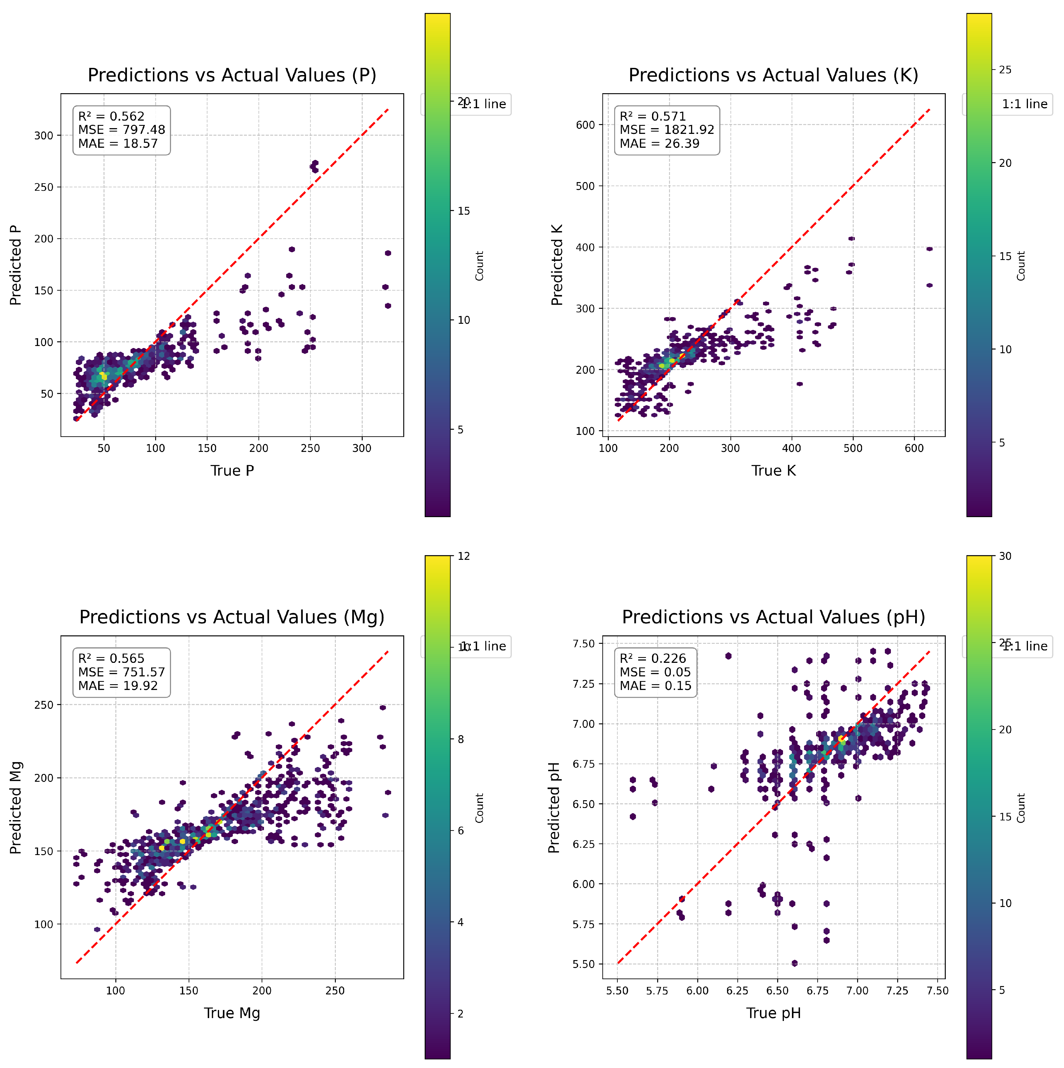
Figure 5.
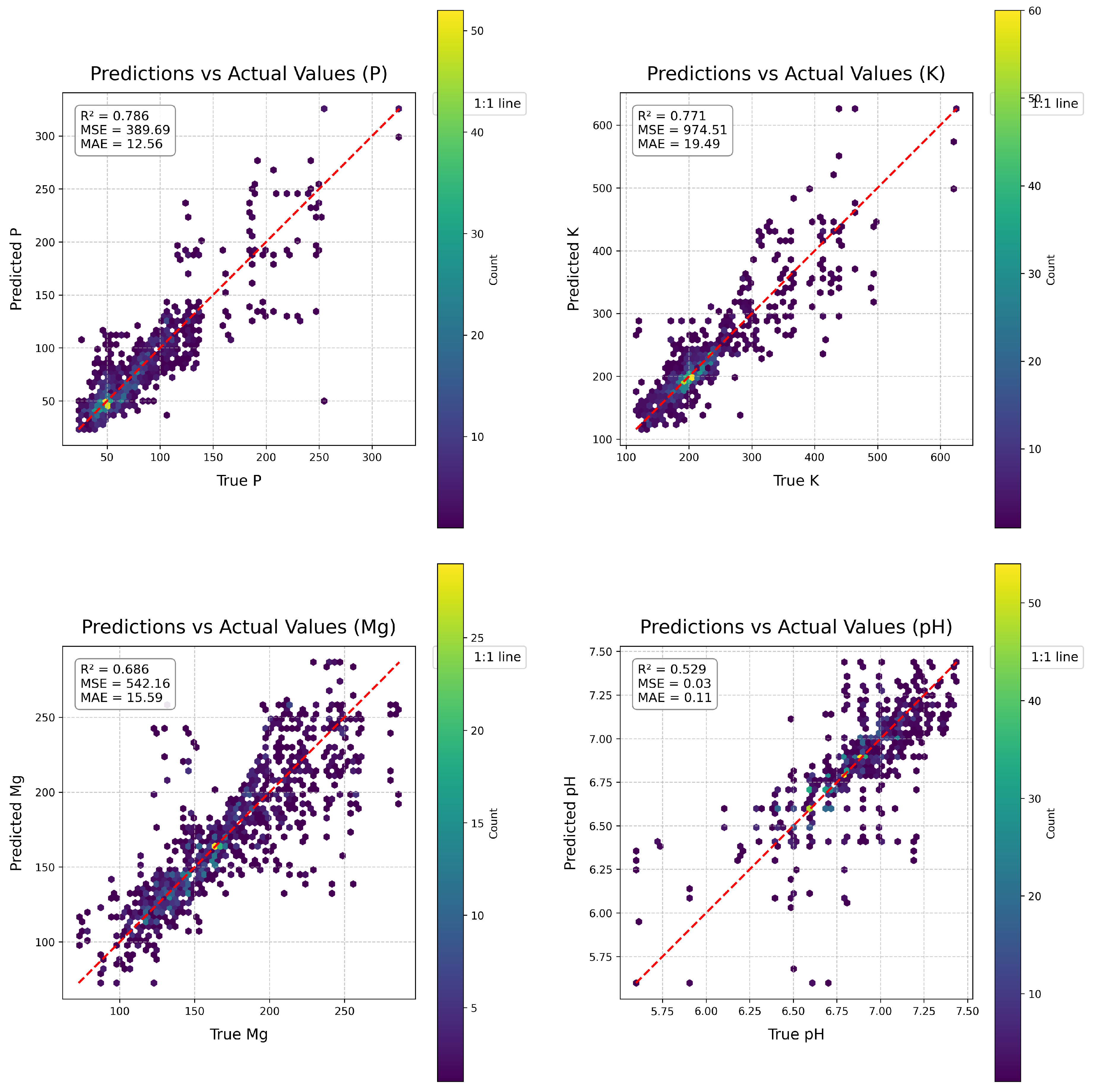
HyperSoilNet Density Plot: HyperSoilNet clusters data more tightly along the identity line than EagleEye does. The upper-range biases are slightly minimised, as evidenced by fewer deviations. The majority of predictions fall along the diagonal, with a high density in the mid-range band.
Figure 5.
HyperSoilNet Density Plot: HyperSoilNet clusters data more tightly along the identity line than EagleEye does. The upper-range biases are slightly minimised, as evidenced by fewer deviations. The majority of predictions fall along the diagonal, with a high density in the mid-range band.
4.1. Evaluation Metrics
The performance of HyperSoilNet is evaluated using metrics aligned with the Hyperview Challenge [23]. The primary metric is Mean Squared Error (MSE), defined as:
where is the true value, is the predicted value, and N is the number of samples. Additionally, a custom evaluation score compares model performance to a baseline prediction, calculated as:
where represents the MSE for the i-th soil parameter using the algorithm, and corresponds to the baseline MSE. These metrics provide a comprehensive assessment of the model’s accuracy and improvement over baseline predictions. Additional metrics including parameter-specific R² values and calibration quality measures are computed to assess model performance across different value ranges.
4.2. Cross-Validation Results
Prior to challenge submission, we evaluated HyperSoilNet through 5-fold cross-validation on the training dataset. Figure 5 shows the scatter plots of predicted versus actual values for each soil property in our cross-validation experiments. These plots reveal several important insights about the performance of our model across different soil properties and value ranges. The model achieved the highest R² for phosphorus pentoxide (P2O5, R² = 0.786) and potassium (K, R² = 0.771), followed by magnesium (Mg, R² = 0.686) and pH (R² = 0.529). This pattern aligns with the spectral separability observed in our analysis of spectral signatures (Figure 2), where P2O5 and K showed more consistent spectral patterns across the NIR-SWIR region than Mg and pH.
Examining the distribution of prediction errors across value ranges reveals that the model generally performs better in the mid-range values for all properties, with higher scatter at extreme values. This pattern is particularly pronounced for pH, where predictions for values below 6.0 and above 7.2 show increased error, likely due to the less frequent occurrence of these extreme values in the training dataset. For nutrient properties (K, P2O5, Mg), the model tends to underestimate high values and overestimate low values, a common regression-to-the-mean pattern observed in many statistical learning models. This suggests that additional techniques might be beneficial for extreme value prediction, such as stratified sampling or specialized loss functions that place greater emphasis on the tails of the distribution.
For comparison, Figure 4 shows the prediction performance of the EagleEyes model [39], which achieved the top score in the original Hyperview Challenge. While both models show similar patterns of error distribution, HyperSoilNet demonstrates improved prediction accuracy, particularly for mid-range values. This improvement is most evident in the tighter clustering along the identity line for K and P2O5, suggesting that our hybrid approach is particularly effective for these nutrients. The comparison also highlights a common challenge in soil property prediction from hyperspectral data: the difficulty in accurately estimating extreme values, which often represent fields with unique conditions or management practices.
4.3. Challenge Results
Following cross-validation, we generated predictions for the withheld test dataset and submitted them to the Hyperview Challenge platform. The evaluation resulted in a score of 0.762 for HyperSoilNet. Table 1 compares our score to other leading entries on the challenge leaderboard. HyperSoilNet achieved a competitive position, outperforming many established approaches in this benchmark task. This strong performance on the external test set validates the generalization capability of our hybrid framework, suggesting that the combination of a pretrained hyperspectral backbone and an ensemble of traditional regressors provides robust predictions across diverse field conditions.
It is important to note that the challenge format prevents us from conducting more detailed analysis of test set performance, such as property-specific error analysis or calibration quality assessment. Our evaluation is therefore primarily based on the aggregate challenge score and cross-validation results. This limitation is inherent to the competition framework, where participants do not have access to the ground truth values for the test set. Nevertheless, the competitive performance on the challenge leaderboard, combined with our thorough cross-validation analysis, provides strong evidence for the effectiveness of our approach in soil property estimation from hyperspectral imagery.

Table 1.
Public Leaderboard of the Hyperview Challenge Scores [23].
Table 1.
Public Leaderboard of the Hyperview Challenge Scores [23].
| S/N | Approach | # Submissions | Score |
|---|---|---|---|
| 1 | EagleEyes | 67 | 0.781 |
| 2 | MOAH | 78 | 0.797 |
| 3 | Black Cat | 32 | 0.803 |
| 4 | WEGIS | 16 | 0.812 |
| 5 | Cap2AIScience | 45 | 0.816 |
| 6 | Predicta | 45 | 0.848 |
| 7 | deep_brain | 6 | 0.853 |
| 8 | u3s_lab | 31 | 0.871 |
| 9 | 32 | 0.875 | |
| 10 | CMG | 10 | 0.877 |
| 11 | HyperSoilNet | 31 | 0.762 |
Note: Best values are in bold.
4.4. Ablation Study
To evaluate the contribution of each component in HyperSoilNet, we conducted an ablation study by systematically altering or removing key parts of the model and assessing their impact on performance using the Hyperview Challenge dataset. Specifically, we focused on the roles of Hyperspectral CNN backbone (HCB) and the machine learning ensemble. Since the test set ground truth was not available, all experiments were performed using stratified 5-fold cross-validation on the training set, with performance measured via the custom score (Equation 11) computed on the validation folds.
We compared the following variants of HyperSoilNet:
- Variant A (Full HyperSoilNet): The complete model, featuring a HCB pre-trained with self-supervised contrastive learning. Features extracted from this backbone are fed into an ensemble of Random Forest, XGBoost, and KNN regressors.
- Variant B (No Pretraining): The HCB is trained from scratch using only the labeled training data to extract features, which are then passed to the same ensemble as Variant A.
- Variant C (HCB): The HCB is fine-tuned for regression using the labeled data, bypassing the ensemble.
- Variants D1-D3 (Individual Regressors): Features from the HCB are used to train each regressor in the ensemble separately: D1 with Random Forest, D2 with XGBoost, and D3 with KNN.
The results are summarized in Table 2.
The results in Table 2 demonstrate that Variant A (Full HyperSoilNet) achieves the best performance with a custom score of . Removing self-supervised pretraining (Variant B) significantly degrades the score to , underscoring the importance of pretraining for learning robust feature representations. Similarly, omitting the ensemble and fine-tuning the HCB yields a score of , suggesting that the ensemble enhances prediction accuracy and robustness beyond what the CNN alone can achieve. Finally, using individual regressors (Variants D1-D3) results in scores ranging from to , all worse than the ensemble, which highlights the advantage of combining multiple regressors to leverage their complementary strengths.
These findings confirm that both the HCB and the machine learning ensemble are integral to the improved perforrmance of HyperSoilNet in estimating soil properties. The pretraining enables effective feature extraction despite limited labeled data, while the ensemble improves prediction quality by integrating diverse regression models.
5. Discussion
5.1. Analysis of Property-Specific Performance
Our cross-validation results reveal interesting patterns in the performance of HyperSoilNet across different soil properties. The varying prediction accuracy can be related to both the spectral characteristics of each property and their natural distribution in the dataset. Phosphorus pentoxide (P2O5) achieved the highest R² (0.786), likely due to its distinct spectral signature in the NIR region. As shown in Figure 2b, fields with different P2O5 levels exhibit systematic differences in reflectance, particularly in bands 80-120. This spectral separability facilitates more accurate predictions by providing clear patterns for the model to learn. Furthermore, P2O5 showed a moderate positive correlation with potassium (r = 0.41), allowing the model to leverage shared information between these properties.
Potassium (K) showed similarly strong predictive performance (R² = 0.771), which may be attributed to its own spectral patterns in the SWIR region and its correlation with P2O5. The spectral signatures for different K levels (Figure 2a) show clear separation, particularly in the range of bands 100-150, providing discriminative features for the model. The correlation between K and P2O5 suggests shared dynamics in the soil that the model can leverage for prediction, potentially through shared features or parameters in the neural network.
Magnesium (Mg) predictions were less accurate (R² = 0.686) despite showing clear spectral separation in Figure 2c. This lower performance may be related to the slight negative correlation with P2O5 (r = -0.10), which might introduce competing spectral patterns that complicate prediction. Additionally, the spectral signature of Mg shows higher variability (wider standard deviation bands) compared to K and P2O5, suggesting greater heterogeneity in how this nutrient manifests in spectral reflectance patterns.
Soil pH was the most challenging property to predict (R² = 0.529), which aligns with its weak correlations with other properties (r = 0.01 to 0.17). Despite showing distinct spectral patterns for different pH levels in Figure 2d, these patterns may be subtler or more easily confounded by other factors such as soil texture or organic matter content, which also influence spectral reflectance in similar wavelength regions. The independent nature of pH compared to the nutrient properties means the model cannot leverage correlations to improve prediction accuracy.
These findings suggest that both the inherent spectral separability and the correlations between properties influence prediction accuracy. Our property-specific ensemble weighting strategy helps mitigate these challenges by optimizing the regressor combination for each property, giving more weight to the algorithms that perform best for that specific soil parameter.
5.2. Advantages of the Hybrid Approach
The superior performance of our hybrid approach compared to both end-to-end deep learning (Variant C in our ablation study) and individual ML regressors (Variants D1-D3) highlights several key advantages of combining these methodologies for soil property estimation. Our hybrid framework leverages complementary strengths from both paradigms: the CNN backbone excels at extracting complex spectral-spatial patterns from raw hyperspectral data, while the ML ensemble provides robust regression with lower risk of overfitting. This combination is particularly valuable given the limited labeled data available in the Hyperview dataset, where end-to-end deep learning approaches would be more prone to overfitting without extensive regularization.
Our property-specific ensemble weighting strategy further enhances this hybrid approach by allowing the model to adapt to the unique characteristics of each soil property. The optimal weights determined through Bayesian optimization reveal that different regressors excel at different properties. XGBoost received higher weights for P2O5 and pH prediction, while Random Forest contributed more significantly to K and Mg prediction. This adaptive weighting can be understood in terms of the statistical properties of each soil parameter and the corresponding modeling strengths of each regressor. For instance, the strength of XGBoost in modeling non-linear relationships and handling outliers makes it particularly effective for pH, which showed the lowest correlation with other properties and more scattered distribution patterns.
The hybrid framework also improves generalization by combining multiple prediction approaches, reducing the risk of overfitting to specific spectral patterns or soil conditions in the training data. This ensemble effect is evident in the strong performance on the challenge test set, which likely contains fields with different characteristics than those in the training set. The diversity of the ensemble members, spanning both tree-based (Random Forest, XGBoost) and distance-based (KNN) methods, ensures that the model can handle a wide range of spectral signatures and soil conditions.
Our ablation results quantify these advantages, showing that the full HyperSoilNet (Variant A) achieved a custom score of 0.683 ± 0.011, significantly outperforming both the CNN-only approach (Variant C, 0.738 ± 0.012) and the best individual regressor (Variant D1, 0.779 ± 0.008). The most dramatic performance drop occurred when removing the pretraining (Variant B, 0.820 ± 0.015), highlighting the critical role of transfer learning from a larger dataset in establishing a strong foundation for soil property prediction.
5.3. Limitations and Future Directions
Despite its promising performance, our approach has several limitations that warrant further investigation in future work. The geographic specificity of the model represents a significant constraint, as it was developed and evaluated on data from Polish agricultural regions. Soil characteristics and spectral signatures vary considerably across different global regions due to differences in parent material, climate, vegetation, and land management practices. This variability may limit the direct transferability of our model to other geographical contexts without adaptation. Future research should validate the approach on diverse datasets spanning different geographical areas and soil types to assess and improve generalization.
The current model also does not account for temporal dynamics in soil spectral signatures, which can vary significantly due to changing moisture conditions, vegetation cover, or management practices throughout growing seasons. Soil moisture, in particular, has a strong influence on spectral reflectance across the entire spectrum, potentially confounding the relationship between reflectance and nutrient content. Incorporating temporal modeling or developing moisture-invariant spectral indices could improve robustness across different seasonal conditions. Multi-temporal datasets that capture the same fields under different moisture conditions would be particularly valuable for this research direction.
From an interpretability perspective, while our spectral analysis provides insights into the relationship between soil properties and spectral signatures, the deep learning component still operates partially as a black box. This limitation can impede adoption by agricultural practitioners who need to understand and trust model predictions. Developing more physically interpretable models that directly relate spectral features to known soil absorption mechanisms would enhance trust and facilitate adoption. Techniques such as layer-wise relevance propagation or gradients visualization could help elucidate which spectral regions most influence predictions for each soil property.
Our current framework focuses on four commonly measured soil properties (K, P2O5, Mg, and pH), but precision agriculture requires monitoring of additional parameters such as nitrogen, organic carbon, soil texture, and moisture. Extending the model to predict these properties would increase its practical utility for comprehensive soil management. This extension would likely require additional labeled data for these properties and potentially different spectral regions or features to capture their unique signatures.
Future research directions to address these limitations include developing soil-specific pretraining techniques that incorporate domain knowledge about spectral absorption features of different soil constituents, exploring physics-informed neural networks that integrate spectroscopic principles directly into the model architecture, investigating active learning approaches to optimize ground sampling strategies based on model uncertainty, creating multi-modal frameworks that combine hyperspectral data with other sensing technologies (e.g., thermal, SAR) for comprehensive soil health assessment, and extending the approach to higher spatial resolution imagery (e.g., from drones) for field-scale precision management. These advancements would further improve the accuracy, interpretability, and practical utility of hyperspectral soil property estimation for precision agriculture and sustainable land management.
5.4. Broader Implications for Precision Agriculture
The capabilities demonstrated by HyperSoilNet have significant implications for precision agriculture and sustainable land management. Accurate remote estimation of soil properties could substantially reduce the need for extensive soil sampling and laboratory analysis, lowering costs and enabling more frequent monitoring. Unlike traditional soil testing based on sparse point samples, hyperspectral imagery provides continuous spatial coverage, revealing field heterogeneity and enabling site-specific management. More precise information about soil nutrient status allows farmers to apply fertilizers only where and when needed, reducing environmental impacts while maintaining productivity.
The approach could be scaled from individual fields to regional or national agricultural monitoring systems, supporting policy decisions and environmental assessment. The soil property maps generated by our approach could feed directly into variable-rate application equipment, enabling automated and optimized resource management. By advancing the accuracy and reliability of non-invasive soil analysis, HyperSoilNet represents a step toward more sustainable and efficient agricultural systems that balance productivity with environmental stewardship.
6. Conclusions
In this work, we introduced HyperSoilNet, a novel hybrid framework that integrates a pretrained hyperspectral CNN backbone with an ensemble of classical regression models to estimate soil properties from hyperspectral imagery. Our approach represents a practical solution for non-invasive soil analysis, directly addressing the challenges posed by limited labeled data and the high dimensionality of hyperspectral images.
The main contributions of this work include the development of a hybrid framework that leverages the complementary strengths of deep learning for feature extraction and traditional machine learning for robust regression, implementation of soil-specific adaptations to the HyperKon backbone, introduction of a property-specific weighted ensemble approach that optimizes prediction performance for each soil parameter individually, and evaluation on the Hyperview Challenge dataset.
Our experiments confirmed that the combination of a pretrained hyperspectral backbone and a carefully designed ML ensemble outperforms both end-to-end deep learning approaches and traditional feature engineering methods. The ablation studies highlighted the importance of each component, with the pretrained backbone providing the foundation for effective feature extraction and the ensemble approach ensuring robust predictions across diverse soil conditions.
Overall, HyperSoilNet contributes a robust and efficient approach for soil property estimation from hyperspectral imagery, supporting more informed decision-making in precision agriculture and sustainable land management.
References
- Tilman, D. Global environmental impacts of agricultural expansion: the need for sustainable and efficient practices. Proceedings of the national Academy of Sciences 1999, 96, 5995–6000. [CrossRef]
- Bongiovanni, R.; Lowenberg-DeBoer, J. Precision agriculture and sustainability. Precision agriculture 2004, 5, 359–387.
- Pradipta, A.; Soupios, P.; Kourgialas, N.; Doula, M.; Dokou, Z.; Makkawi, M.; Alfarhan, M.; Tawabini, B.; Kirmizakis, P.; Yassin, M. Remote sensing, geophysics, and modeling to support precision agriculture—Part 1: Soil applications. Water 2022, 14, 1158.
- Abdulraheem, M.I.; Zhang, W.; Li, S.; Moshayedi, A.J.; Farooque, A.A.; Hu, J. Advancement of remote sensing for soil measurements and applications: A comprehensive review. Sustainability 2023, 15, 15444. [CrossRef]
- Omia, E.; Bae, H.; Park, E.; Kim, M.S.; Baek, I.; Kabenge, I.; Cho, B.K. Remote sensing in field crop monitoring: A comprehensive review of sensor systems, data analyses and recent advances. Remote Sensing 2023, 15, 354. [CrossRef]
- Ram, B.G.; Oduor, P.; Igathinathane, C.; Howatt, K.; Sun, X. A systematic review of hyperspectral imaging in precision agriculture: Analysis of its current state and future prospects. Computers and Electronics in Agriculture 2024, 222, 109037. [CrossRef]
- Cheng, C.; Zhao, B. Prospect of application of hyperspectral imaging technology in public security. In Proceedings of the International Conference on Applications and Techniques in Cyber Security and Intelligence ATCI 2018: Applications and Techniques in Cyber Security and Intelligence. Springer, 2019, pp. 299–304.
- Brisco, B.; Brown, R.; Hirose, T.; McNairn, H.; Staenz, K. Precision agriculture and the role of remote sensing: a review. Canadian Journal of Remote Sensing 1998, 24, 315–327. [CrossRef]
- Clark, R.N.; Swayze, G.A.; Livo, K.E.; Kokaly, R.F.; Sutley, S.J.; Dalton, J.B.; McDougal, R.R.; Gent, C.A. Imaging spectroscopy: Earth and planetary remote sensing with the USGS Tetracorder and expert systems. Journal of Geophysical Research: Planets 2003, 108. [CrossRef]
- Bioucas-Dias, J.M.; Plaza, A.; Camps-Valls, G.; Scheunders, P.; Nasrabadi, N.; Chanussot, J. Hyperspectral remote sensing data analysis and future challenges. IEEE Geoscience and remote sensing magazine 2013, 1, 6–36. [CrossRef]
- Gewali, U.B.; Monteiro, S.T.; Saber, E. Machine learning based hyperspectral image analysis: a survey. arXiv preprint arXiv:1802.08701 2018.
- Yu, S.; Jia, S.; Xu, C. Convolutional neural networks for hyperspectral image classification. Neurocomputing 2017, 219, 88–98.
- Liu, L.; Awwad, E.M.; Ali, Y.A.; Al-Razgan, M.; Maarouf, A.; Abualigah, L.; Hoshyar, A.N. Multi-Dataset Hyper-CNN for Hyperspectral Image Segmentation of Remote Sensing Images. Processes 2023, 11, 435. [CrossRef]
- Li, S.; Song, W.; Fang, L.; Chen, Y.; Ghamisi, P.; Benediktsson, J.A. Deep learning for hyperspectral image classification: An overview. IEEE Transactions on Geoscience and Remote Sensing 2019, 57, 6690–6709. [CrossRef]
- Chhapariya, K.; Buddhiraju, K.M.; Kumar, A. CNN-Based Salient Object Detection on Hyperspectral Images Using Extended Morphology. IEEE Geoscience and Remote Sensing Letters 2022, 19, 1–5. [CrossRef]
- Vali, A.; Comai, S.; Matteucci, M. Deep learning for land use and land cover classification based on hyperspectral and multispectral earth observation data: A review. Remote Sensing 2020, 12, 2495. [CrossRef]
- Sun, H.; Zheng, X.; Lu, X. A supervised segmentation network for hyperspectral image classification. IEEE Transactions on Image Processing 2021, 30, 2810–2825. [CrossRef]
- Signoroni, A.; Savardi, M.; Baronio, A.; Benini, S. Deep learning meets hyperspectral image analysis: A multidisciplinary review. Journal of imaging 2019, 5, 52. [CrossRef]
- Jia, S.; Jiang, S.; Lin, Z.; Li, N.; Xu, M.; Yu, S. A survey: Deep learning for hyperspectral image classification with few labeled samples. Neurocomputing 2021, 448, 179–204. [CrossRef]
- Chen, T.; Kornblith, S.; Norouzi, M.; Hinton, G. A simple framework for contrastive learning of visual representations. In Proceedings of the International conference on machine learning. PMLR, 2020, pp. 1597–1607.
- Wang, Y.; Albrecht, C.M.; Braham, N.A.A.; Mou, L.; Zhu, X.X. Self-supervised learning in remote sensing: A review. IEEE Geoscience and Remote Sensing Magazine 2022, 10, 213–247. [CrossRef]
- Li, T.; Zhang, X.; Zhang, S.; Wang, L. Self-supervised learning with a dual-branch ResNet for hyperspectral image classification. IEEE Geoscience and Remote Sensing Letters 2022, 19, 1–5. [CrossRef]
- Nalepa, J.; Le Saux, B.; Longépé, N.; Tulczyjew, L.; Myller, M.; Kawulok, M.; Smykala, K.; Gumiela, M. The Hyperview Challenge: Estimating Soil Parameters from Hyperspectral Images. In Proceedings of the 2022 IEEE International Conference on Image Processing (ICIP). IEEE, 2022, pp. 4268–4272.
- Wang, Y.; Zou, B.; Chai, L.; Lin, Z.; Feng, H.; Tang, Y.; Tian, R.; Tu, Y.; Zhang, B.; Zou, H. Monitoring of soil heavy metals based on hyperspectral remote sensing: A review. Earth-Science Reviews 2024, p. 104814. [CrossRef]
- Patel, A.K.; Ghosh, J.K.; Sayyad, S.U. Fractional abundances study of macronutrients in soil using hyperspectral remote sensing. Geocarto International 2022, 37, 474–493. [CrossRef]
- Ge, Y.; Thomasson, J.A.; Morgan, C.L.; Searcy, S.W. VNIR diffuse reflectance spectroscopy for agricultural soil property determination based on regression-kriging. Transactions of the ASABE 2007, 50, 1081–1092. [CrossRef]
- Zelikman, E.; Carmina, E. The spectral response characteristics of the soils and their possible estimation by using partial least square regression (PLSR) analysis. International journal of geomatics and geosciences 2013, 3, 438–453.
- Jain, S.; Sethia, D.; Tiwari, K.C. A critical systematic review on spectral-based soil nutrient prediction using machine learning. Environmental Monitoring and Assessment 2024, 196, 699. [CrossRef]
- Jia, P.; Shang, T.; Zhang, J.; Sun, Y. Inversion of soil pH during the dry and wet seasons in the Yinbei region of Ningxia, China, based on multi-source remote sensing data. Geoderma Regional 2021, 25, e00399. [CrossRef]
- Choudhury, M.R.; Christopher, J.; Das, S.; Apan, A.; Menzies, N.W.; Chapman, S.; Mellor, V.; Dang, Y.P. Detection of calcium, magnesium, and chlorophyll variations of wheat genotypes on sodic soils using hyperspectral red edge parameters. Environmental Technology & Innovation 2022, 27, 102469. [CrossRef]
- Zhong, L.; Guo, X.; Xu, Z.; Ding, M. Soil properties: Their prediction and feature extraction from the LUCAS spectral library using deep convolutional neural networks. Geoderma 2021, 402, 115366. [CrossRef]
- Tsimpouris, E.; Tsakiridis, N.L.; Theocharis, J.B. Using autoencoders to compress soil VNIR–SWIR spectra for more robust prediction of soil properties. Geoderma 2021, 393, 114967. [CrossRef]
- Singh, S.; Kasana, S.S. Quantitative estimation of soil properties using hybrid features and RNN variants. Chemosphere 2022, 287, 131889. [CrossRef]
- Liu, Y.; Shen, L.; Zhu, X.; Xie, Y.; He, S. Spectral Data-Driven Prediction of Soil Properties Using LSTM-CNN-Attention Model. Applied Sciences 2024, 14, 11687. [CrossRef]
- Cao, L.; Sun, M.; Yang, Z.; Jiang, D.; Yin, D.; Duan, Y. A novel transformer-CNN approach for predicting soil properties from LUCAS Vis-NIR spectral data. Agronomy 2024, 14, 1998. [CrossRef]
- Pham, N.T.; Rakkiyapan, R.; Park, J.; Malik, A.; Manavalan, B. H2Opred: a robust and efficient hybrid deep learning model for predicting 2’-O-methylation sites in human RNA. Briefings in Bioinformatics 2024, 25, bbad476. [CrossRef]
- Aljohani, A.; Aburasain, R.Y. A hybrid framework for glaucoma detection through federated machine learning and deep learning models. BMC Medical Informatics and Decision Making 2024, 24, 115. [CrossRef]
- Remzan, N.; Hachimi, Y.E.; Tahiry, K.; Farchi, A. Ensemble learning based-features extraction for brain mr images classification with machine learning classifiers. Multimedia Tools and Applications 2024, 83, 57661–57684. [CrossRef]
- Kuzu, R.S.; Albrecht, F.; Arnold, C.; Kamath, R.; Konen, K. Predicting soil properties from hyperspectral satellite images. In Proceedings of the 2022 IEEE International Conference on Image Processing (ICIP). IEEE, 2022, pp. 4296–4300.
- Mehlich, A. Mehlich 3 soil test extractant: A modification of Mehlich 2 extractant. Communications in soil science and plant analysis 1984, 15, 1409–1416. [CrossRef]
- Hanlon, E.; Johnson, G. Bray/Kurtz, Mehlich III, AB/D and ammonium acetate extractions of P, K and Mg in four Oklahoma soils. Communications in soil science and plant analysis 1984, 15, 277–294.
- Ayuba, D.L.; Guillemaut, J.Y.; Marti-Cardona, B.; Mendez, O. HyperKon: A Self-Supervised Contrastive Network for Hyperspectral Image Analysis. Remote Sensing 2024, 16. [CrossRef]
- Lee, D.T.; Yamamoto, A. Wavelet analysis: theory and applications. Hewlett Packard journal 1994, 45, 44–44.
Table 2.
Average results for the Ablation Study.
| Variant | Description | Custom Score (CV) |
|---|---|---|
| A | Full HyperSoilNet | |
| B | No Pretraining + Ensemble | |
| C | HCB | |
| D1 | HCB. + Random Forest | |
| D2 | HCB. + XGBoost | |
| D3 | HCB. + KNN |
Note: Best values are in bold.
Disclaimer/Publisher’s Note: The statements, opinions and data contained in all publications are solely those of the individual author(s) and contributor(s) and not of MDPI and/or the editor(s). MDPI and/or the editor(s) disclaim responsibility for any injury to people or property resulting from any ideas, methods, instructions or products referred to in the content. |
© 2025 by the authors. Licensee MDPI, Basel, Switzerland. This article is an open access article distributed under the terms and conditions of the Creative Commons Attribution (CC BY) license (http://creativecommons.org/licenses/by/4.0/).
Copyright: This open access article is published under a Creative Commons CC BY 4.0 license, which permit the free download, distribution, and reuse, provided that the author and preprint are cited in any reuse.


