
Submitted:
06 May 2025
Posted:
07 May 2025
You are already at the latest version
Abstract
To solve the problem of active suspension control effect reduction in trucks due to the change of vehicle mass after loading, this paper designs an active suspension hybrid controller for trucks with online estimation of vehicle mass. A multi-degree-of-freedom coupling dynamics model of the vehicle integrated with mass estimator is established, the online estimation of the vehicle mass is estimated in real time based on the recursive least squares method with forgetting factor, the mass estimation is integrated with the Linear Quadratic Regulator(LQR) of active suspension control, and the system is validated by simulation under the real-time change of mass. The results show that the active suspension hybrid controller integrated with the online estimation of the vehicle mass has a better control effect, can adapt to the real-time change of the mass of the truck and ensure the effectiveness of the control system.
Keywords:
active suspension
; least squares method
; vehicle mass estimation
; Linear Quadratic Regulator control
1. Introduction
With the help of advanced sensors, controllers and actuators, the active suspension can sense the vehicle motion state and road surface condition in real time[1], and actively adjust the suspension parameters, which can greatly improve the driving performance of the vehicle under various working conditions.
In the field of modern logistics and transportation, the control method of the active suspension system of the truck has been a research hotspot for many years[2,3].The frame control system usually uses fixed vehicle parameters, but the mass of the truck will change greatly due to the different loads, if the fixed vehicle parameters are still used to control the vehicle suspension, it will inevitably affect to a large extent the truck's stability and maneuverability[4,5]. Therefore, it is necessary to integrate with real-time online mass estimation in the design of suspension controllers to guarantee the performance of trucks under different load conditions.
For vehicle mass estimation, this is usually done based on a longitudinal vehicle dynamic model. Early studies mostly used simplified longitudinal dynamics models combined with least squares (LS) or recursive least squares (RLS) for parameters estimation[6,7]. Such methods reduce computational complexity by simplifying the model structure, but have limited ability to deal with nonlinear characteristics and parameter coupling problems.
To solve the estimation accuracy problem of nonlinear system, some scholars realized state estimation by constructing nonlinear longitudinal dynamics model and improved real-time performance through forward Eulerian method of discretization[8]. Some other scholars realized online estimation of vehicle mass by constructing a nonlinear longitudinal model integrated with a state observer, which improved the speed tracking accuracy and control robustness under complex working conditions [9].
To address the problem of multi-source data utilization under complex working conditions, some scholars have improved the mass estimation accuracy under complex working conditions by separating the coupling relationship between mass and slope through the RLS algorithm with forgetting factor based on longitudinal dynamics model [10]. Some scholars improved the estimation accuracy by utilizing the correlation between high-frequency driving force and acceleration signal based on the mass-slope decoupling strategy of longitudinal dynamics equation[11]. Some other scholars further improved the data accuracy by integrating multi-sensor data through the parameter updating mechanism of the optimized longitudinal dynamics model with co-processing [12]. All these methods are used to enhance the estimation accuracy under complex operating conditions by extending the model dimensions or data integration strategies.
Suspension system is a key component of automobile, and its effective control can significantly improve driving stability and ride comfort[13].Today, there are numerous suspension control methods, including the common canopy damping control[14], fuzzy control [15,16], optimal control[17,18], and deep learning control[19].Within optimal control algorithms, Linear Quadratic Regulator (LQR) is capable of carrying out multi-objective optimization of the controlled system[20]. Multi-objective optimization can greatly improve the vibration characteristics of automotive suspension systems [21,22,23].Good vibration characteristics can effectively suppress the bumps generated by the road roughness[24], which is the core factor to ensure the stability of the vehicle, reduce the body shaking and impact, and is of great significance to improve the overall performance and safety of the vehicle[25]. The application of LQR to suspension systems can better balance vehicle driving stability and ride comfort[26].
In this paper, the modeling of a suspension control system integrated with the estimation of vehicle mass is carried out with full consideration of the effect of mass variation on suspension control. A seven-degree-of-freedom vehicle active suspension model considering road excitation, lateral and longitudinal acceleration is established, and a active suspension hybrid controller with a hybrid Linear Quadratic Regulator is proposed. Under the condition of ensuring that the remaining control variables do not change much, the vehicle LQR control strategy focusing on the dynamics response and body attitude control is designed and analyzed through numerical simulation. The body vertical acceleration, body pitch angle, body roll angle, suspension dynamic deflection and tire dynamic deformation are used as evaluation metrics. The obtained simulation results are compared with the uncontrolled passive suspension and the LQR controller without integrated with mass estimation(original controller)in the time and frequency domains to verify the effectiveness of the control strategy.
2. Multi-Degree-of-Freedom Coupling Dynamics Model of Vehicle
To consider the lateral, longitudinal, and vertical characteristics, a vehicle mass coupling dynamics model with multiple degrees of freedom is established, which includes a total of seven degrees of freedom, including the vertical, pitch, and lateral movements of the body and the vertical movement of the unsprung mass, as shown in Figure 1.
According to Newton's second law, the vertical vibration equation at the center of mass is
where, is the sprung mass, is the vertical displacement of the center of mass of the sprung mass, footnote , is the left front wheel, left rear wheel, right front wheel, and right rear wheel, respectively, is the total suspension forces of the -th wheel. The total suspension forces expressed by is the sum of the elastic force, the damping force, and the suspension actuator force, which can be expressed as
where, is the suspension stiffness of the -th wheel, is the suspension damping of the -th wheel, and and are the unsprung mass vertical displacement and the sprung mass vertical displacement of the -th wheel, respectively.
Under the effect of inertial acceleration, the equations of motion for the rolling and pitching of the sprung mass can be expressed respectively as
where, g is the acceleration of gravity, and are the lateral and pitch moment of inertia of the sprung mass, respectively, and are the distances from the center of the vehicle mass to the front and rear axes, as well as the front half shaft base and rear half shaft base, respectively. and are the longitudinal and lateral accelerations of the center of the vehicle mass, respectively, and are the distance from the center of mass of the sprung mass to the pitch and roll axes, respectively, and are the roll and pitch angles of the sprung mass, respectively.
The vibration equation for an unsprung mass is
where, is the unsprung mass of the -th wheel, is the tire stiffness of the -th wheel, and the road input of the -th wheel.
When the roll angle and pitch angle are varied in a very small range, the displacements of the -th wheel's sprung mass are respectively
Define
The vibration equations for the sprung mass and unsprung mass can be simplified to matrix form
To design the controller, the above equation is expressed in matrix form as a state equation of the form
where, selection of state variables
output variable
actuator force input
the vehicle vehicle's perturbation vector is
where, the vehicle's system state matrixes is
3. Hybrid Control System Architecture for Active Suspension Integrated with Mass Estimation
For trucks, the mass of the load will greatly affect the control effect of the active suspension controller, which is basically stable and unchanged during the driving process with stability[27,28]. The algorithm is used to estimate the vehicle mass and then adjust the active suspension controller by the estimated vehicle mass, to achieve a more optimal effect on the vehicle suspension control. The framework of the vehicle control strategy is shown in Figure 2. The overall framework is divided into three parts, part 1 is vehicle mass estimation module, part 2 is actuator force calculation module, and part 3 is vehicle multi-degree-of-freedom(multi-doff) model module, respectively. Part 1 estimates the vehicle mass by the recursive least squares method with forgetting factor, and outputs the vehicle mass; part 2 recognizes the vehicle mass and real-time state variables by the online LQR controller, and calculates the optimal solution of the actuator force, and part 3 accepts the actuator force outputted by the online LQR controller, and transmits the real-time driving state variables of the vehicle to part 1 and part 2.
4. Design of Active Suspension Hybrid Controller
4.1. Module For Recursive Least Squares with Forgetting Factor for Vehicle Mass Estimation
4.1.1. Vehicle Mass Estimation Model
According to Newton's second law, the longitudinal motion equation of the vehicle is as follows
expanding the equation gives
where, is the longitudinal driving force, is the rolling resistance, is the air resistance, is the ramp resistance, is the mass of the vehicle, is the longitudinal speed of the vehicle, is the actual torque input from the engine to the transmission, is the transmission ratio, is the main gearbox ratio, is the mechanical efficiency of the driveline, is the rolling radius of the wheels, is the air density, is the wind resistance coefficient, is the windward surface area, is the roadway gradient, is the road roll resistance coefficient.
The equation is transformed as follows
4.1.2. Recursive Least Squares Algorithm with Forgetting Factor
Recursive least squares (RLS) uses the criterion of least squares (Least squares), which is based on the principle of using exponentially weighted error sum of squares to minimize the model estimation error, and the RLS algorithm has better convergence and tracking ability, and the computational volume is small[29]. The forgetting factor can dilute or enhance the influence of historical data on the current estimation and improve the adaptability of the algorithm. The effect of on historical data is shown in Table 1.
In this paper, we set the size of the forgetting factor to = 0.95.
According to longitudinal vehicle dynamic model, the input-output recursive equation of mass estimation of recursive least squares with forgetting factor(FFRLS) is established
where, is the input, which is the measurable data vector; is the output of the system; is the parameter to be estimated, and the parameter to be estimated in this paper is the vehicle mass .
From the longitudinal dynamic equation, it can be obtained
The steps of FFRLS are as follows
(1) Solve for parameter identification gain
(2) Update parameter identification
(3) Update the recognition error
where, is the parameter identification gain at moment ; is the covariance matrix at moment ; and is the unit matrix.
The estimated vehicle mass , sprung mass , and unsprung mass are related as
where, the unsprung mass is a fixed preset value and the sprung mass, can be derived from the mass estimator after estimating the vehicle mass .
4.2. Module for LQR-Based Actuator Force Calculation
The Linear Quadratic Regulator (LQR) controller is a full state feedback controller that minimizes the error by means of an objective function and a suitable gain matrix to allow the system to achieve better performance. The LQR cost function is chosen as follows
where the input and output weight matrices are respectively, as follows
In the weight matrix, ~ are the state variable weight coefficients, and ~ are the actuator force weight coefficients. and reflect the relative importance of outputs and inputs. By modifying the above equation, the standard form of LQR control can be obtained as
included among these
By solving the Riccati equation in the following generalized form
obtain the positive definite solution matrix P. The feedback gain matrix of the controller is
Finally, the actuator force is obtained as
4.3. Hybrid Control Logic
First, the hybrid LQR controller accepts the vehicle mass estimated by FFRLS, and calculates the vehicle's system state matrixes in real time based on the estimated mass as well as the preset basic parameters, and inputs the system state matrixes into the LQR controller to compute the controller's feedback gain matrix in real time, and then computes the optimal actuator force from the state parameters of the vehicle as shown in (27).
To prevent the estimated mass change from causing the feedback gain matrix of LQR to change too frequently, a mass change suppression module is used, quality change suppression module is used, This module introduces the absolute percentage error (APE) metric of the estimated mass to determine whether the is updated or not
where, is the current vehicle mass used to calculate the feedback gain matrix for LQR, is the estimated vehicle mass at the current moment, and is the threshold value, where the value of remains unchanged when ; conversely is updated.
5. Comparative Simulation Analysis
The vehicle system is subjected to complex maneuvering excitation and random road excitation in practice. In order to conform to the practical operating condition of the vehicle, the combined working condition that can respond to the lateral, longitudinal and vertical motions of the system is designed. The combined working condition can stimulate the coupling of vehicle motions in each degree of freedom, such as the vertical vibration of unsprung mass and sprung mass, and the coupling motion of body pitch and roll.
To verify the effectiveness of the design strategy, the passive suspension, original controller and hybrid controller are analysed by numerical simulation using random road excitation respectively. The random road excitation adopts the filtered white noise time-domain road input model[30], which is as follows
where is the lower cut-off frequency of is the uniformly distributed white noise of the -th wheel, and is the road roughness coefficient.
In this paper, we use class B pavement as the random road input, the roughness coefficient of class B pavement is , and the lower cut-off frequency is taken as .
5.1. Vehicle Simulation Parameter Selection
The parameters of the vehicle used for simulation are shown in Table 2.
5.2. Dynamic Response and Body Attitude Analysis Integrated with Online Estimation of Vehicle Mass
First, the validity of the vehicle mass estimation algorithm is verified, and then the effects of vehicle dynamics response and body attitude control are compared between passive suspension, LQR controller without integrated with vehicle mass estimation (original controller) and LQR controller with integrated with vehicle mass estimation (hybrid controller).
The vehicle longitudinal velocity and longitudinal acceleration are shown in Figure 3 and Figure 4, respectively.
5.2.1. Vehicle Mass Estimation Simulation Analysis
Vehicle mass estimation result are shown in Figure 5.
As shown in Figure 5, the mass estimation algorithm designed in this paper can effectively estimate the vehicle mass within a short time and converge the error to within 5%. To enable the mass estimation value to respond better in the hybrid controller, the mass estimation value is averaged every 5s, and the effect is shown in Figure 6.
5.2.2. Vehicle Dynamic Response and Body Attitude Analysis
To study the effect of load change on suspension control, this paper adopts the variable load condition, the load is changed from 1200 kg to 2000 kg and then the system is laterally and longitudinally loaded in which the vehicle's lateral and longitudinal acceleration is shown in Figure 7.
Since the mass estimation takes some time to converge, the dynamic response and body attitude analysis is performed below for 20-40 seconds.
Time Domain Response Analysis
Table 3 shows the comparison of the root mean square plant for each evaluation metric.
Figure 8, Figure 9 and Figure 10 show the time-domain response curves characterising the body attitude control quantities body pitch angle, body roll angle and suspension dynamic deflection. Table 3 shows the comparison of the root mean square plant for each evaluation metric.
Combined with Figure 8, Figure 9 and Figure 10 and Table 3, it can be seen that compared with the passive suspension, hybrid controller reduces the rms root-plant of body roll angle and pitch angle by 72.80% and 7.20% , respectively, and the suspension dynamic deflection is reduced by an average of 36.91%. Compared with the original controller, hybrid controller maintains similar rms root-plant of body roll angle and pitch angle, while the suspension dynamic deflection is reduced by an average of 3.26%, achieving better control of the vehicle body attitude.
Figure 11 and Figure 12 show the time domain response curves characterizing the dynamic response to body vertical acceleration and tire dynamic deformation.
As can be seen from Figure 11 and Figure 12, the hybrid controller reduces the body vertical acceleration and tire dynamic deformation compared to passive suspension. Combined with the comparison of the rms values in Table 3, compared to the passive suspension, the hybrid controller reduced the body vertical acceleration by 7.95% and the original controller reduced the body vertical acceleration by 18.33%, the hybrid controller reduced the tire dynamic deformation by an average of 3.17% and the original controller increased the tire dynamic deformation by an average of 2.74%. The result shows that the hybrid controller has less variation in tire dynamic deformation.
The results show that the hybrid controller proposed in this paper, for the passive suspension, all the metrics are reduced; for the original controller, although the body vertical acceleration is deteriorated, the degree of deterioration is within the acceptable range, and when the vehicle mass is 2000 kg, the safety is especially important, and the control of the suspension dynamic deformation and tire dynamic deformation is more critical, and if the original controller is used for the control of the vehicle, it is a deviation from the performance of the preset required control.
Frequency Domain Response Analysis
The frequency domain response curve of body vertical acceleration is shown in Figure 13.
From the frequency domain analysis in Figure 13, it can be seen that, compared with the passive suspension, the hybrid controller body vertical acceleration response has a significant reduction at the first-order resonance peak and little change at the second-order resonance peak; compared with the original controller, the hybrid controller body vertical acceleration response is slightly higher at the first-order resonance peak and at the second-order resonance peak, but it is still within a reasonable range.
The frequency domain response curve of suspension dynamic deflection is shown in Figure 14.
From the frequency domain analysis in Figure 14, it can be seen that, the hybrid controller suspension dynamic deflection response is reduced at both the first-order resonance peak and the second-order resonance peak, compared with the passive suspension and the original controller. Where, for the passive suspension, the hybrid controller suspension dynamic deflection response is significantly reduced at the first-order resonance peak, and for the original controller, the hybrid controller suspension dynamic deflection response is significantly reduced at the second-order resonance peak, and the result demonstrates that the hybrid controller is more effective in the control of the suspension dynamic deflection.
The frequency domain response curve of tire dynamic deformation is shown in Figure 15.
From the frequency domain analysis in Figure 15, it can be seen that, compared with the passive suspension, both the original controller and the hybrid controller tire dynamic deformation responses are significantly reduced at the first-order resonance peaks, where the original controller is slightly better than the hybrid controller; at the second-order resonance peaks, the original controller tire dynamic deformation response is significantly higher compared with the passive suspension, whereas the hybrid controller tire dynamic deformation response does not change much compared with the passive suspension.
Comprehensive analysis of the above, in the case of the total mass of the truck is 2t, the comfort of the hybrid controller has a lower degree of deterioration, but greatly guarantee the safety performance of the vehicle in the case of heavy loads, and the results show that the hybrid controller has a very good adaptability for the quality of different cases of the truck.
5.3. Analysis of Actuator Force and Efficiency
Figure 16 shows a comparison of the actuator force for the original controller and the hybrid controller.
As shown in Figure 16a, the amplitude of the actuator force of the original controller is in general larger and less efficient than that of the hybrid controller. As shown in Figure 16b, the original controller causes a high frequency actuator force component to be output from the active suspension, whereas the hybrid controller's high frequency component is greatly reduced, and such improvement reduces the requirement of the active suspension actuator speed, which is beneficial to the design of the active suspension actuator. In conclusion, hybrid controller not only makes the design of active suspension less difficult but also enables the utilization and performance of active suspension to be improved compared with the original controller.
6. Conclusions
For the active suspension control problem of truck, in this paper, a seven-degree-of-freedom suspension model of the vehicle is established, and a control algorithm based on hybrid controller is proposed, and simulation is used to verify the effectiveness of the model and the control strategy, and the following conclusions are drawn.
(1)In this paper, a hybrid controller for active suspension of trucks integrated with online estimation of vehicle mass is proposed. Compared with the original controller, the hybrid controller can adapt to the real-time change of the vehicle mass, and has a better control effect to ensure the effectiveness of the control system.
(2)According to the characteristics of the parameter changes in the vehicle driving process, based on the longitudinal vehicle dynamic using the FFRLS and simulation test verification, the final mass estimation results of the error are less than 5%.
(3)Simulink co-simulation results show that under the combined working condition of responding to the lateral, longitudinal and vertical motions of the system, compared with the original controller, in the time domain, the root-mean-square (RMS) plant of the suspension dynamic deflection and tire dynamic deformation of the hybrid controller is reduced by 3.26% and 5.91% on average, respectively, achieving good control of the body dynamic response and body attitude under heavy load condition. In the frequency domain characteristics, the suspension dynamic deflection response tire dynamic deformation induced by external excitation of the hybrid controller is generally better than that of the original controller, which optimizes the body attitude frequency response. On the other hand, although some metrics deteriorated in the time and frequency domains, the overall global optimization of comfort and attitude stability can be achieved.
Overall, the hybrid controller is well optimized for suspension dynamic deflection, and tire dynamic deformation compared to the original suspension. This result shows the good adaptability of the hybrid controller for trucks with different masses.
Author Contributions
Conceptualization, C.M.; methodology, C.M., Y.H.; resources, Y.H. and D.Z.; data curation, C.M.; writing—original draft preparation, C.M. and W.Z.; writing—review and editing, Y.H. and C.M.; supervision, Y.H.; project administration, Y.H. All authors have read and agreed to the published version of the manuscript.
Funding
This research was funded by The National Natural Science Foundation of China (Grant No.52302470; Grant No.52462053), The Ganpo Talent Support Program-Leading Academic and Technical Personnel in Major Disciplines of Jiangxi Province (Grant No.20232BCJ23091), The Natural Science Foundation of Jiangxi Province (Grant No.20232BAB214092; Grant No.20224BAB214045), The Key R & D Program of Jiangxi Province (Grant No.20232BBE50010;Grant No.20232BBE50009), The Open bidding for selecting the best candidates Program of Nanchang (Grant No. 2022JBGS001), and The 03 Special Program and 5G Project of Jiangxi Province (Grant No.20232ABC03A30).
Data Availability Statement
The data supporting this study’s findings are available from the corresponding authors upon reasonable request.
Acknowledgments
The authors thank the participants, institutions, editors, and reviewers for enabling us to conduct this research.
Conflicts of Interest
The authors declare no conflicts of interest.
References
- Theunissen, J.; Tota, A.; Gruber, P.; Dhaens, M.; Sorniotti, A. Preview-based Techniques for Vehicle Suspension Control: a State-of-the-Art Review[J]. Annual Reviews in Control, 2021. [CrossRef]
- Kimball, J.B., DeBoer, B., & Bubbar, K. (2024). Adaptive control and reinforcement learning for v1ehicle suspension control: A review. Annual Reviews in Control, 58, 100974. ISSN 1367 - 5788.
- Yu, M.; Evangelou, S.A.; Dini, D. Advances in Vehicle Suspension Systems. Engineering, 2024, 33(2), 160 - 177. [CrossRef]
- Hassan, M.A.; Abdelkareem, M.A.A.; Moheyeldein, M.M.; Elagouz, A.; Tan, G. Advanced Study of Tire Characteristics and Their Influence on Vehicle Lateral Stability and Untripped Rollover Threshold[J]. Alexandria Engineering Journal, 2020, 59(3), 1613 - 1628. ISSN 1110 - 0168.
- Cordoş, N.; Todoruţ, A. Influences of the Suspensions Characteristics on the Vehicle Stability[C]. In Proceedings of the 4th International Congress of Automotive and Transport Engineering (AMMA 2018), Cham, Switzerland, 30 September 2018.
- Liu, L.; Ren, Y.J.; Sha, W.H.; et al. Grade Recognition for Electric Vehicles With Vehicle Mass Estimation[J]. Journal of Jilin University (Engineering and Technology Edition), 2024, 1-10. [CrossRef]
- Chen, P.; Wei, C.; Soler-Nou, A.; et al. User Comfort and Naturalness of Automated Driving: The Effect of Vehicle Kinematic and Proxemic Factors on Subjective Response[J]. Applied Ergonomics, 2025, 122, 104397.
- Lei, Y.L.; Fu, Y.; Liu, K.; et al. Vehicle Mass and Road Grade Estimation Based on Extended Kalman Filter[J]. Transactions of the Chinese Society for Agricultural Machinery, 2014, 45(11), 9-13+8.
- Yang, M.; Tian, J. Longitudinal and Lateral Stability Control Strategies for ACC Systems of Differential Steering Electric Vehicles[J]. Electronics, 2023, 12(19), 4178.
- Liao, Y.S.; Hu, Z.M.; Jia, H.B.; et al. Vehicle Mass and Road Grade Estimation Based on Longitudinal-Lateral Dynamics Coupling[J]. Automotive Engineer, 2024, (10), 1-7. [CrossRef]
- Chu, W.B. Distributed Electric Drive Vehicle Dynamic State Parameter Observation and Driving Force Coordination Control[D]. Tsinghua University, Beijing, China, 2013.
- Kim, H.; Lee, S.; Cho, C. Vehicle Mass Estimation Using Sensor Fusion and a Robust Extended Kalman Filter[J]. IEEE Transactions on Vehicular Technology, 2018, 67(9), 8277-8287.
- Liu, S.J. Development of Automotive Active Control Suspension System[J]. Automotive Technology, 1996, (03), 1-4.
- Zhang, L.; Zhang, J.Q.; Peng, Z.Z.; et al. Improved Skyhook Damping Control Algorithm for Vehicle Semi-Active Suspension[J]. Chinese Journal of Automotive Engineering, 2015, 37(08), 931-935. [CrossRef]
- Fang, X.B.; Chen, W.W.; Wu, L.; et al. Fuzzy Control Technology and Its Application in Automotive Semi-Active Suspensions[J]. Journal of Mechanical Engineering, 1999, (03): 99-101.
- Chen, J.P.; Feng, W.T.; Guo, W.S.; et al. Variable - Universe Fuzzy Control Strategy for Semi - Active Suspension of Vehicle Magnetorheological Damper[J]. Transactions of the Chinese Society for Agricultural Machinery, 2011, 42(05): 7-13+19.
- Yu, F., & Guo, K.H. Optimal Adaptive and Self - Tuning Control of Vehicle Suspensions[J]. Automotive Engineering, 1998, (04): 193-200+205. [CrossRef]
- Dong, B. Research on the Vehicle Model with Optimal Control for Active Suspension[J]. Automotive Engineering, 2002, (05): 422-425. [CrossRef]
- Kou, F.R.; Hu, K.L.; Chen, R.C.; et al. Model Predictive Control of Active Suspension Based on ResNeSt Network Pavement State Recognition[J]. Control and Decision, 2024, 39(06), 1849-1858. [CrossRef]
- Kumar, L.; Kumar, P.; Dhillon, S.S. A Multiobjective Optimization Approach for Linear Quadratic Gaussian/Loop Transfer Recovery Design[J]. Optimal Control Applications and Methods, 2020. [CrossRef]
- Kader, A.M.; El-Gamal, H.A.; Abdelnaeem, M. Influence of Pneumatic Tire Enveloping Behavior Characteristics on the Performance of a Half Car Suspension System Using Multi-Objective Optimization Algorithms[J]. Alexandria Engineering Journal, 2024, 107, 298-316. ISSN 1110-0168.
- Liu, W.; Shi, W.K.; Gui, L.M.; et al. Multi-Objective Optimization of Suspension Systems Based on Ride Comfort and Handling Stability[J]. Journal of Jilin University (Engineering and Technology Edition), 2011, 41(05), 1199-1204. [CrossRef]
- Zuo, S.G.; Jiang, W.X.; Wu, X.D.; et al. Optimization of Vibration Transfer Characteristics for Torsion Beam Suspension of Electric Vehicles Based on ISIGHT[J]. Journal of Jilin University (Engineering and Technology Edition), 2015, 45(05), 1381-1387. [CrossRef]
- He, L.Q.; Pan, Y.J.; He, Y.S.; Li, Z.X.; Królczyk, G.; Du, H.P. Control Strategy for Vibration Suppression of a Vehicle Multibody System on a Bumpy Road[J]. Mechanism and Machine Theory, 2022, 174, 104891. ISSN 0094-114X.
- Sun, T.; Xu, G.; Chai, L.A. Study on the Road Model With Four-Wheel Non-Stationary Random Excitations[J]. Automot. Eng, 2013, 35, 868-872.
- Rong, J.L.; Deng, Z.K.; He, L.; et al. Time-Domain Simulation and Optimization of Ride Comfort for Vehicle Active Suspension[J]. Transactions of Beijing Institute of Technology, 2022, 42(1), 46-52. [CrossRef]
- Li, Y.N.; Zheng, L.; Chen, D.B. Optimal Active Control Based on Truck Body Suspension[J]. Journal of Chongqing Jiaotong University (Natural Science Edition), 2015, 34(4), 130-133+142.
- Fang, C.J.; Zhao, H.; Huang, K.; et al. Linear Quadratic Optimal Control for Automotive Semi-Active Suspension[J]. Automotive Industry Research, 2012, (11), 44-47.
- Widrow, B.; Stearns, S.D. Adaptive Signal Processing; Prentice-Hall: Englewood Cliffs, USA, 1985.
- Tao, S.; Guaihong, X.; Lingjiang, C. A Study on the Road Model With Four-Wheel Non-Stationary Random Excitations[J]. Automotive Engineering, 2013, 35, 868-872. [CrossRef]
Figure 1.
Multi-degree-of-freedom coupling dynamics model.
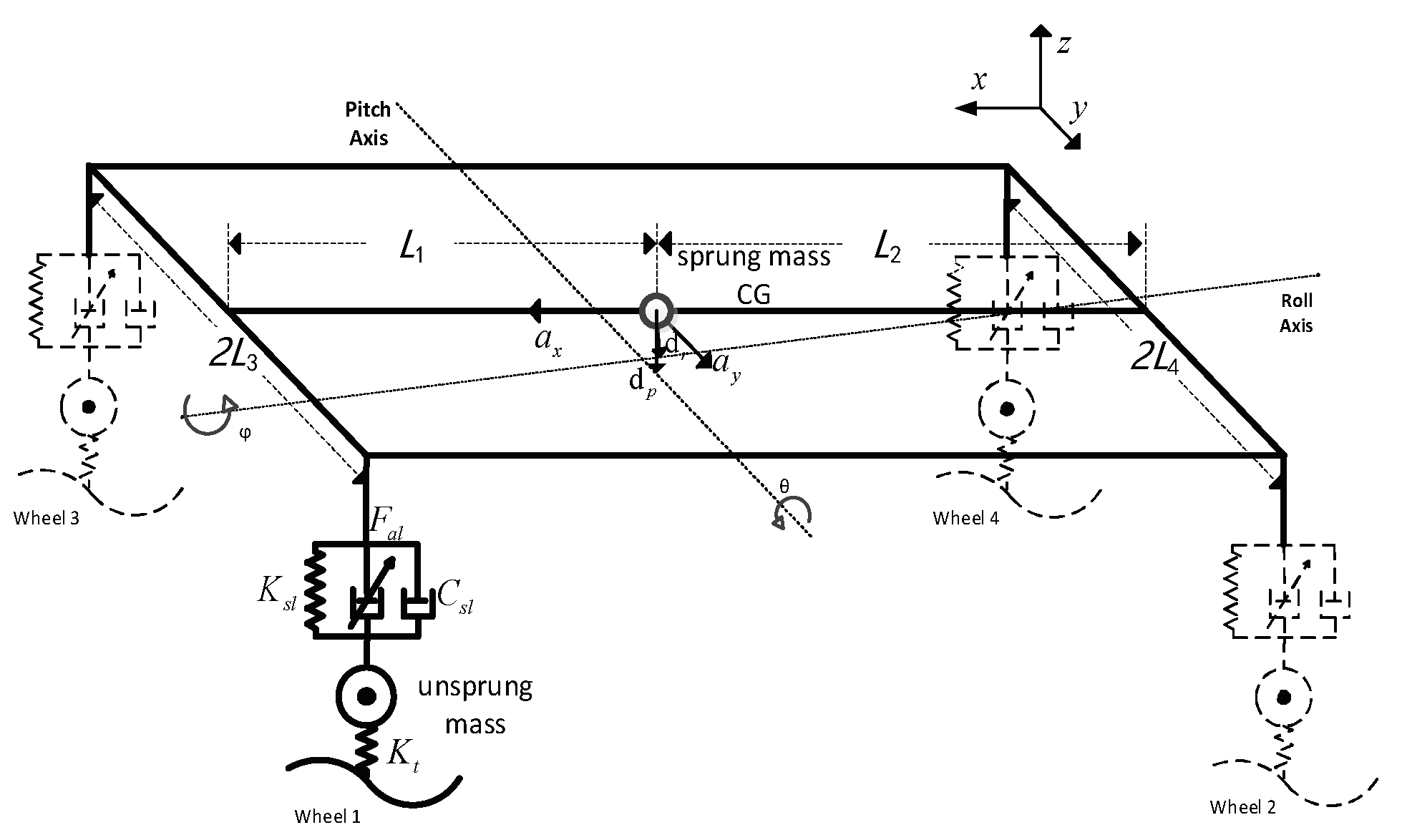
Figure 2.
Architecture for Hybrid Controller.
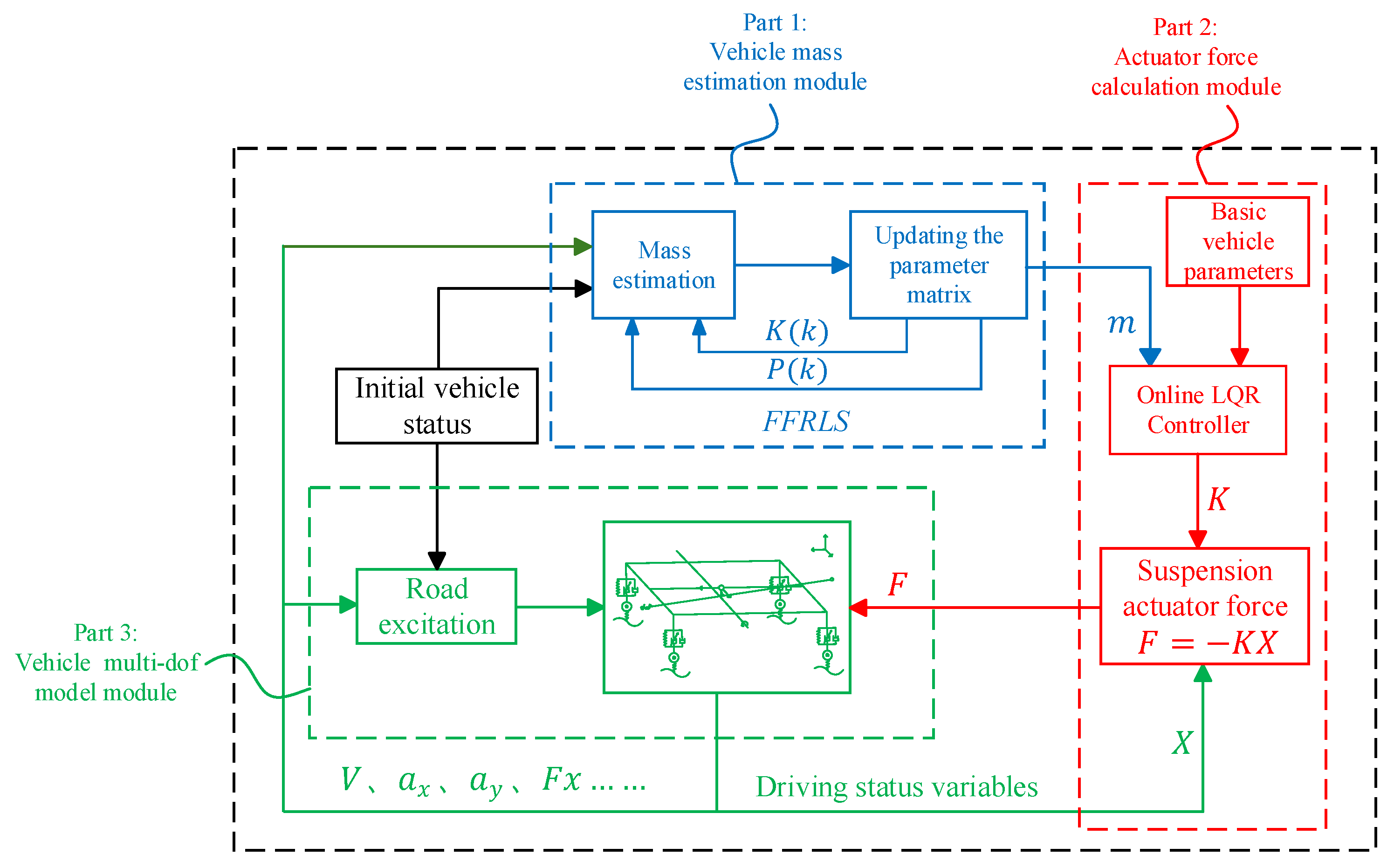
Figure 3.
Vehicle longitudinal speed.
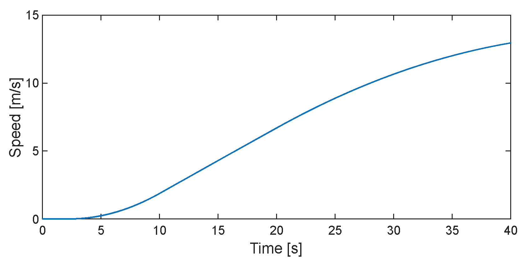
Figure 4.
Vehicle longitudinal acceleration.
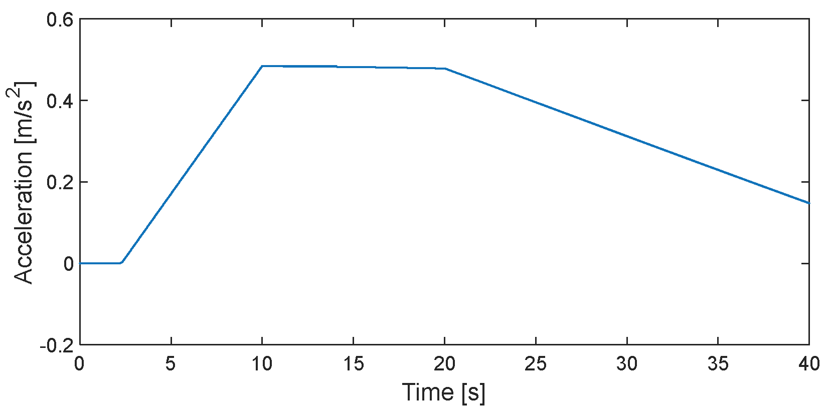
Figure 5.
Vehicle mass estimation result.
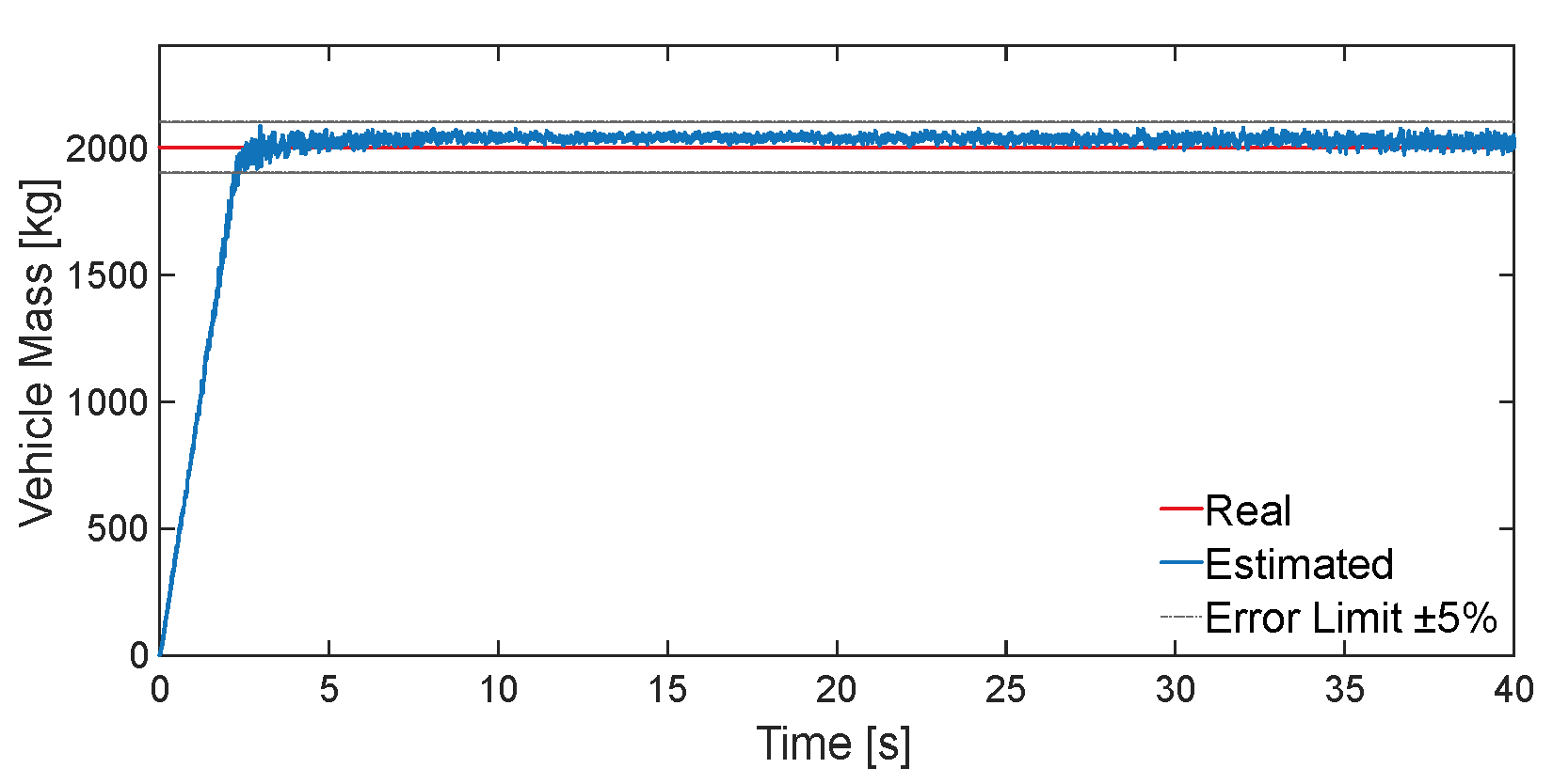
Figure 6.
Mean-processed mass estimation result.
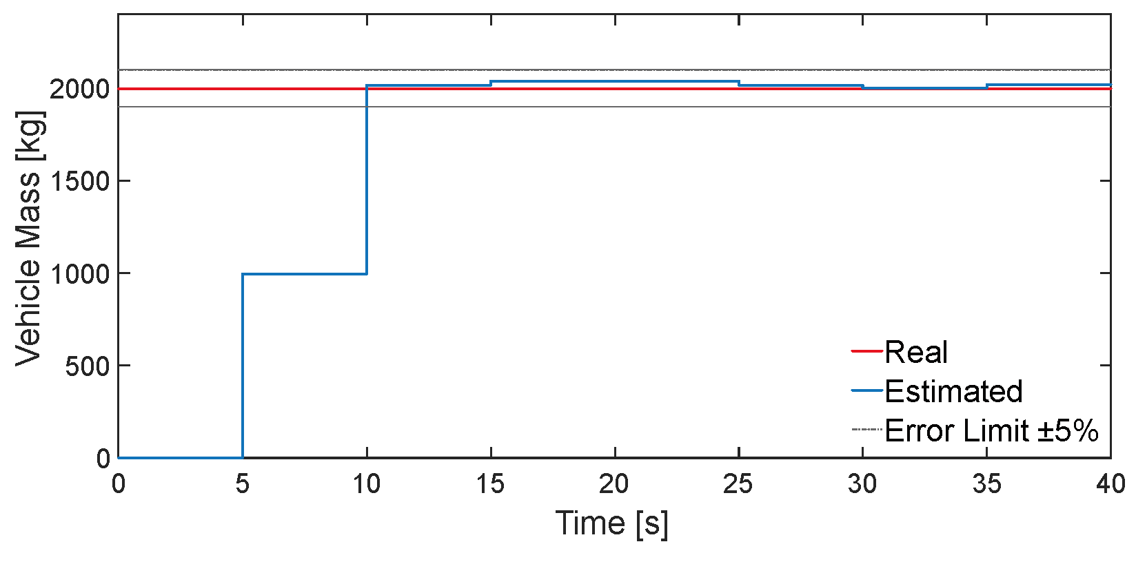
Figure 7.
Vehicle lateral and longitudinal acceleration.
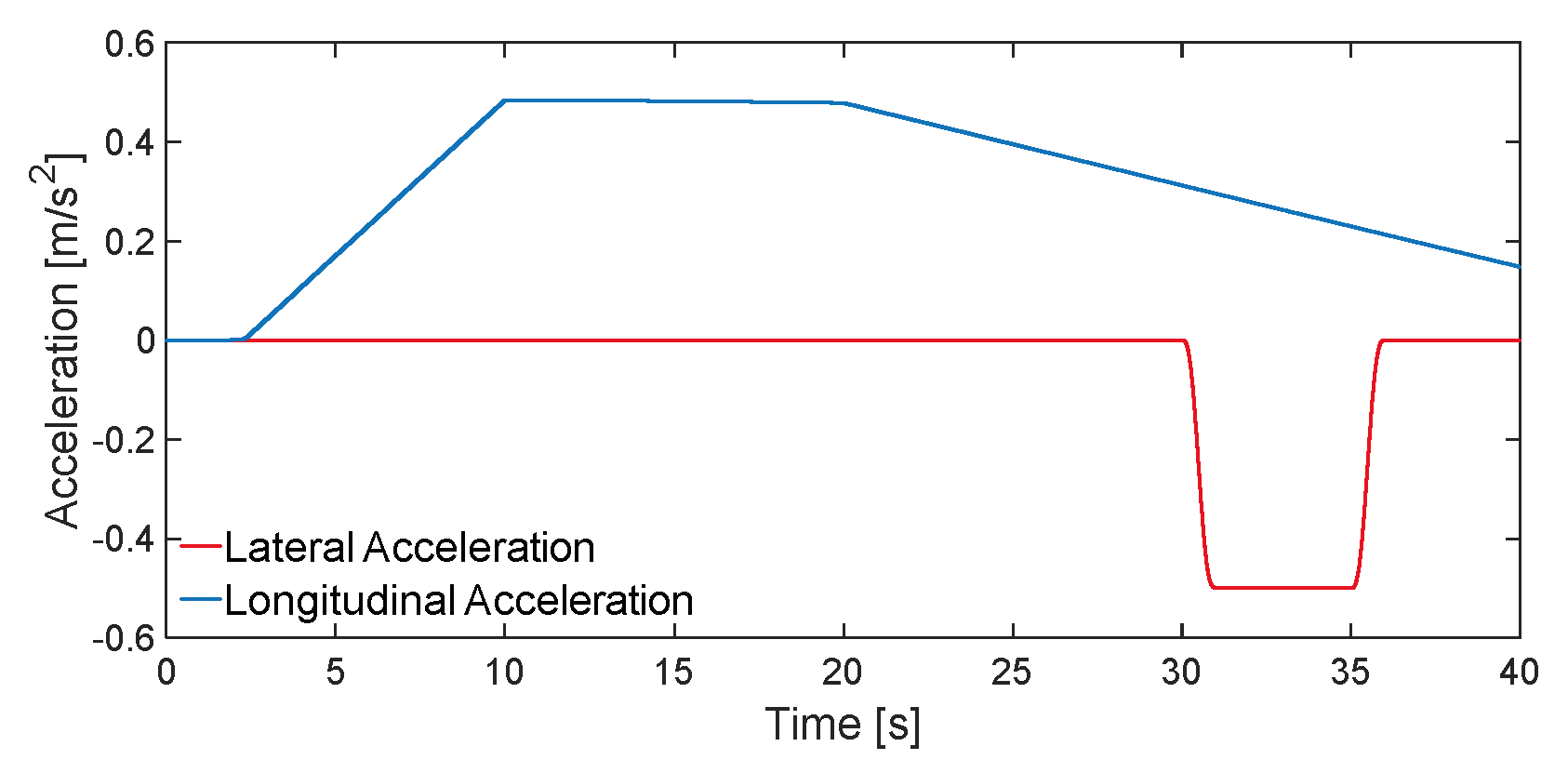
Figure 8.
Time domain response curve of body pitch angle.
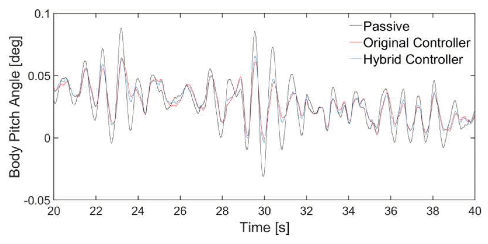
Figure 9.
Time domain response curve of body roll angle.
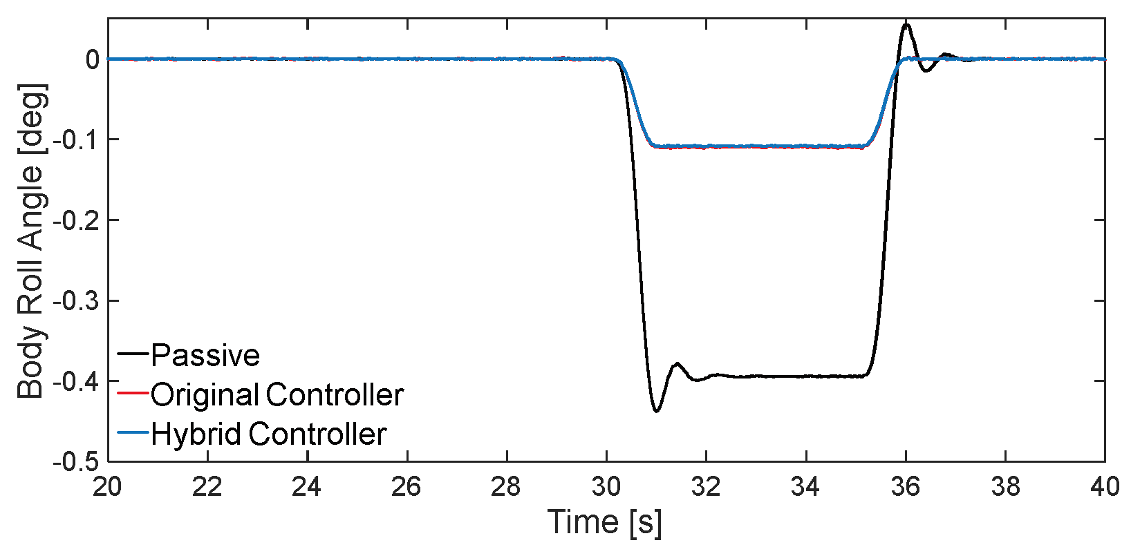
Figure 10.
Time domain response curve of suspension dynamic deflection: (a) Wheel 1; (b) Wheel 2; (c) Wheel 3; (d) Wheel 4.
Figure 10.
Time domain response curve of suspension dynamic deflection: (a) Wheel 1; (b) Wheel 2; (c) Wheel 3; (d) Wheel 4.
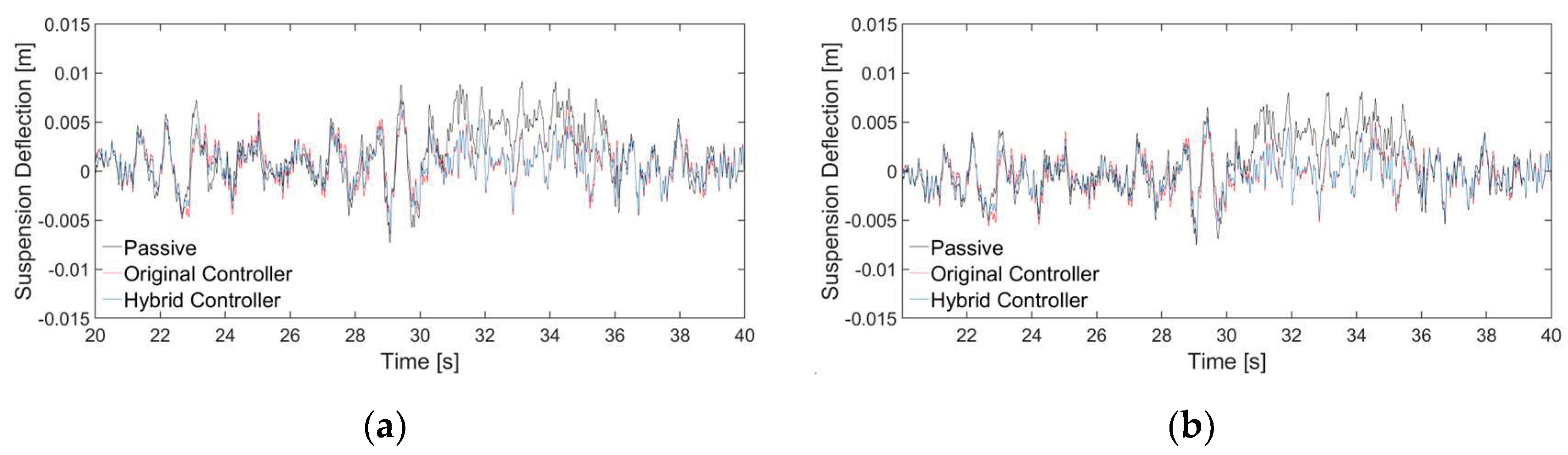
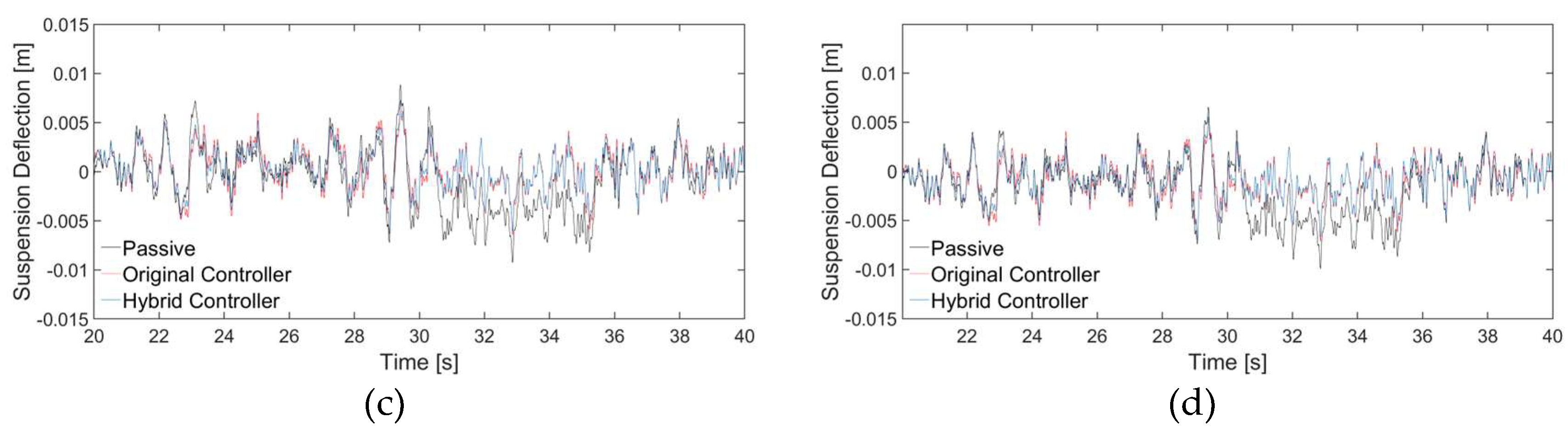
Figure 11.
Time domain response curve of body vertical acceleration.
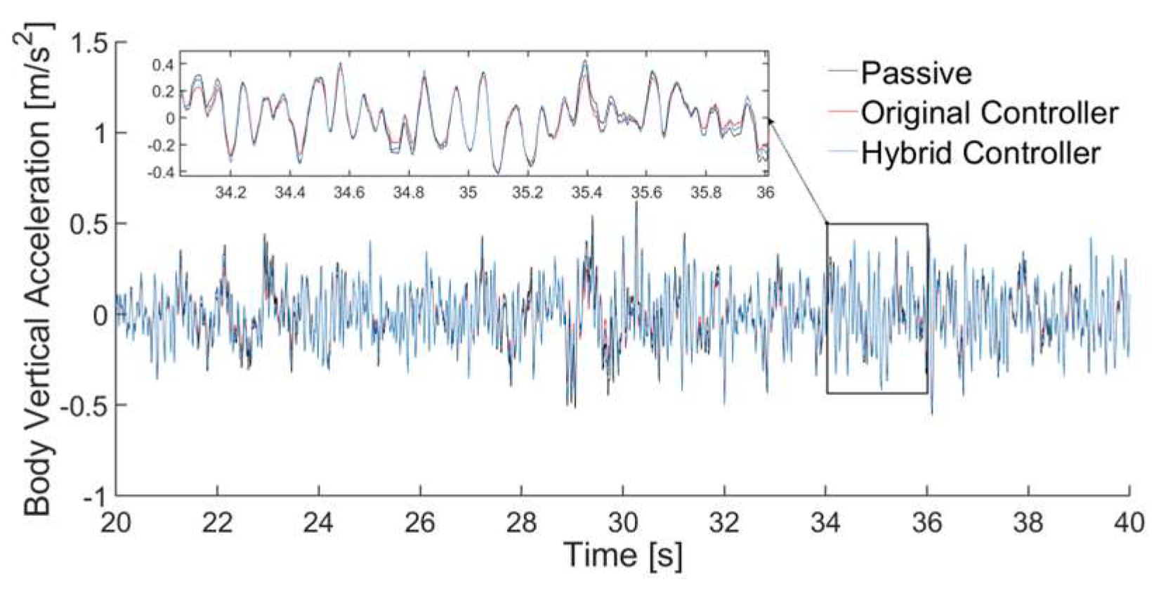
Figure 12.
Time domain response curve of tire dynamic deformation: (a) Wheel 1; (b) Wheel 2; (c) Wheel 3; (d) Wheel 4.
Figure 12.
Time domain response curve of tire dynamic deformation: (a) Wheel 1; (b) Wheel 2; (c) Wheel 3; (d) Wheel 4.
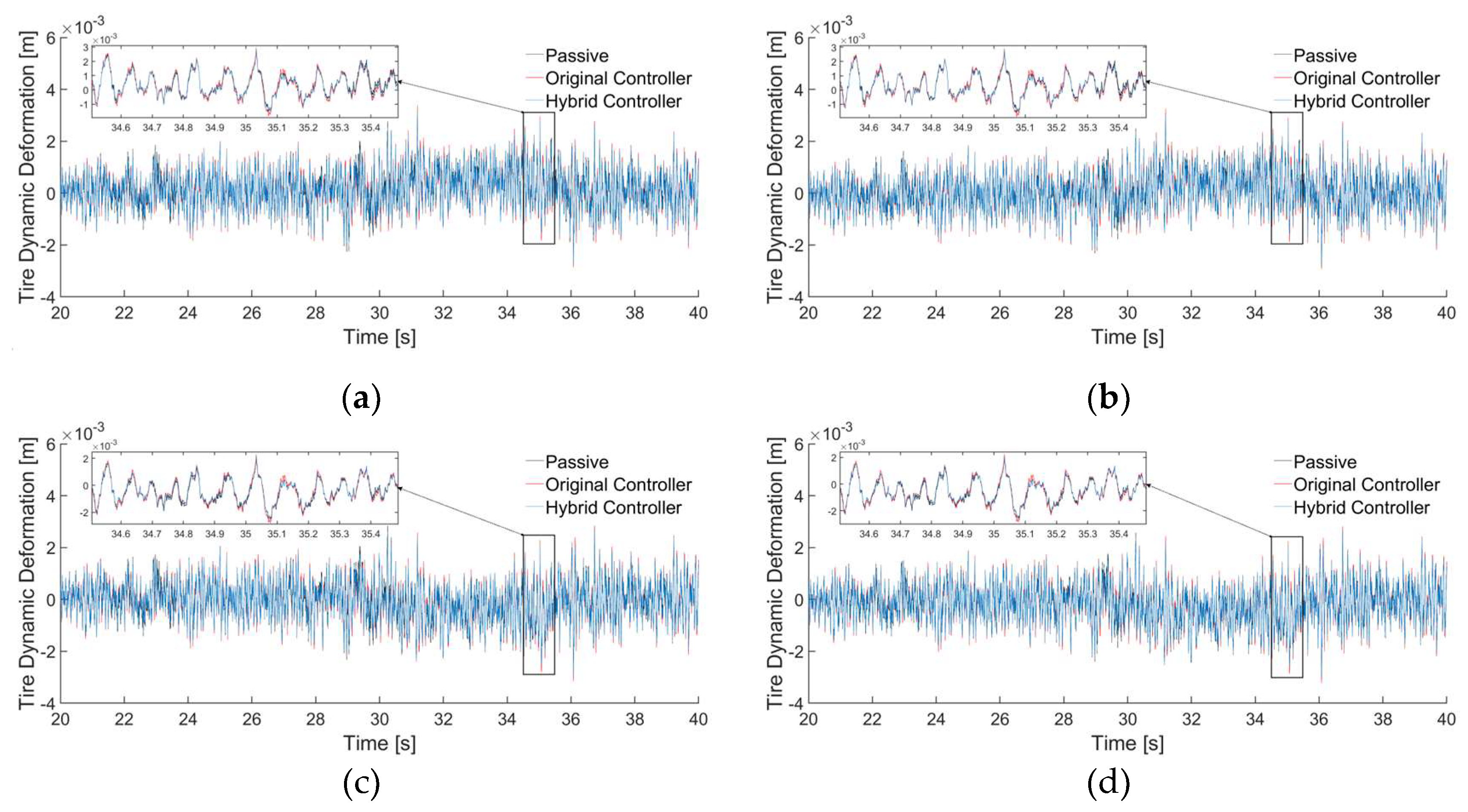
Figure 13.
Frequency domain response curve of body vertical acceleration.
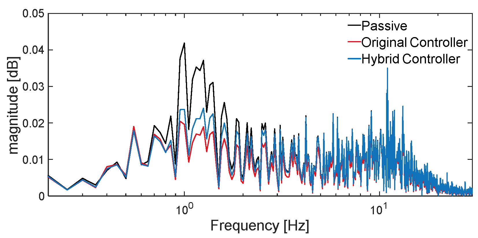
Figure 14.
Frequency domain response curve of suspension dynamic deflection: (a) Wheel 1; (b) Wheel 2; (c) Wheel 3; (d) Wheel 4.
Figure 14.
Frequency domain response curve of suspension dynamic deflection: (a) Wheel 1; (b) Wheel 2; (c) Wheel 3; (d) Wheel 4.
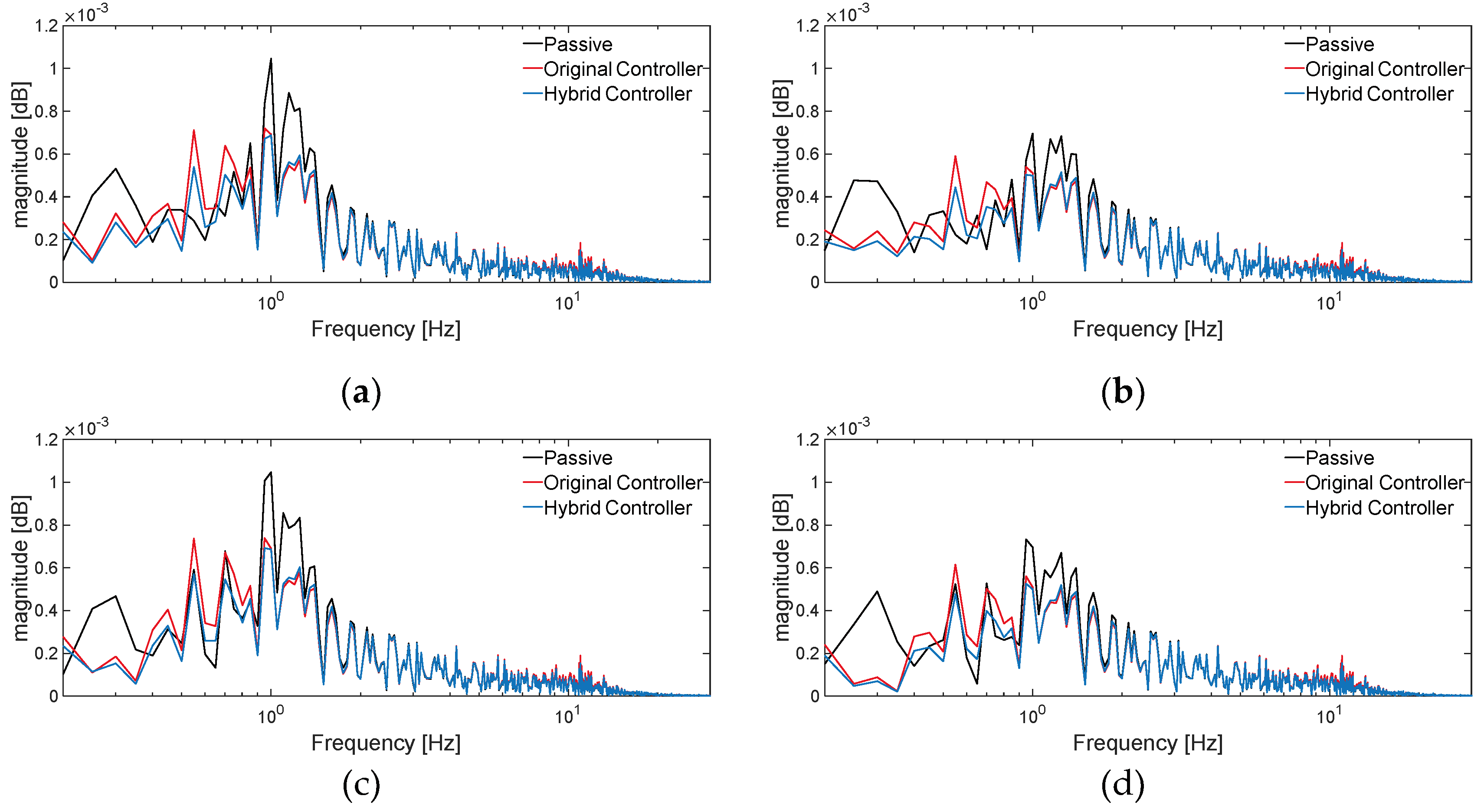
Figure 15.
Frequency domain response curve of tire dynamic deformation: (a) Wheel 1; (b) Wheel 2; (c) Wheel 3; (d) Wheel 4.
Figure 15.
Frequency domain response curve of tire dynamic deformation: (a) Wheel 1; (b) Wheel 2; (c) Wheel 3; (d) Wheel 4.
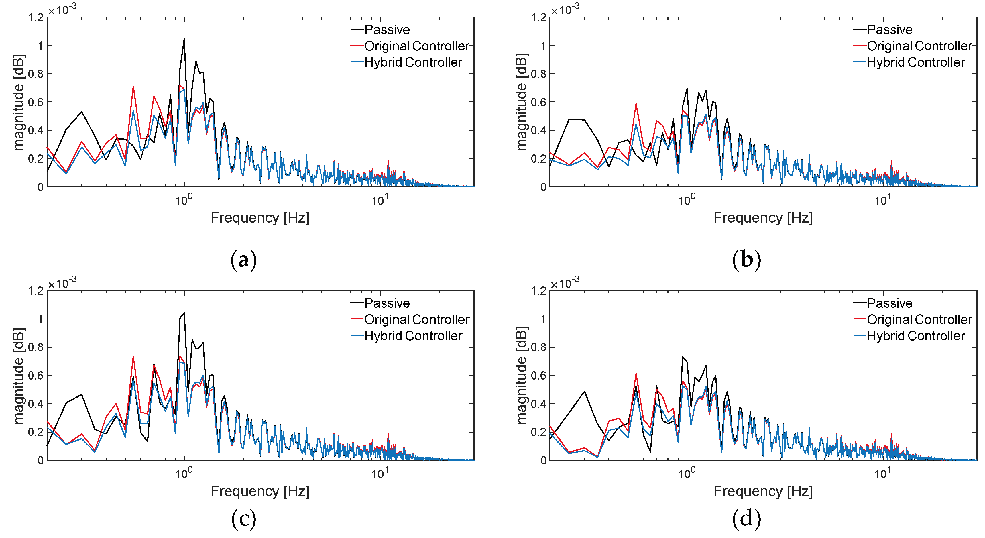
Figure 16.
Comparison of actuator force: (a) Time domain comparison; (b) Frequency domain comparison.
Figure 16.
Comparison of actuator force: (a) Time domain comparison; (b) Frequency domain comparison.
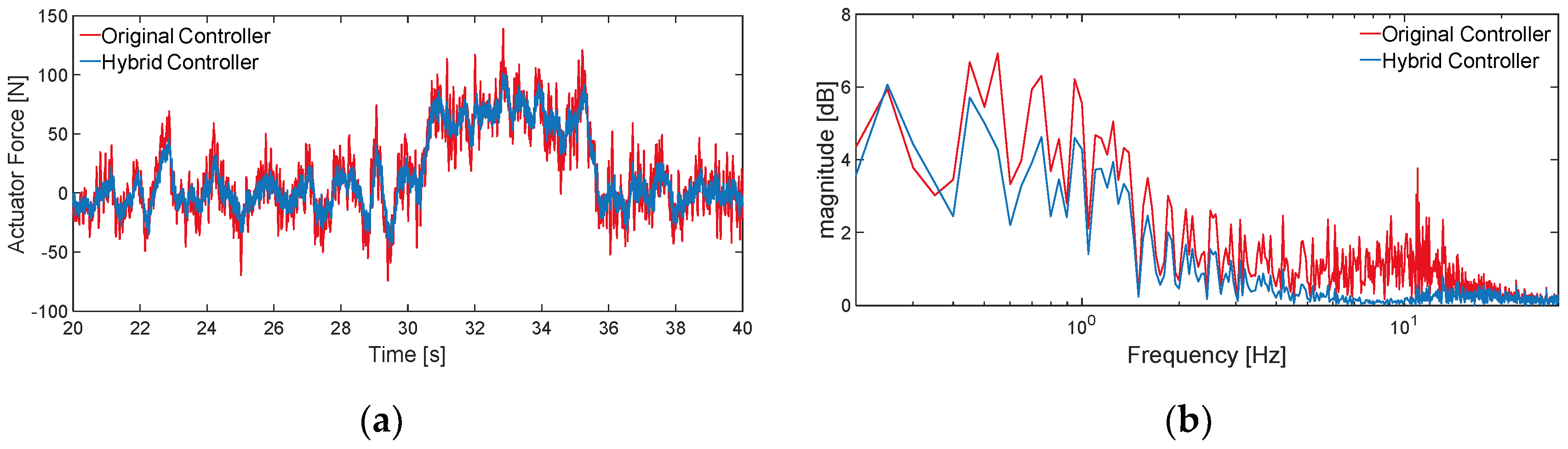

Table 1.
Effect of forgetting factors on historical data
| Effect on historical data | |
|---|---|
| 0<<1 | diluted |
| =1 | unaffected |
| >1 | enhanced |
Table 2.
Vehicle parameters.
| Parameters | Value | Unit |
|---|---|---|
| Nominal vehicle mass | 1200 | kg |
| Vehicle actual mass | 2000 | kg |
| Air density | 1.18 | kg·m⁻³ |
| Windward area | 1.6 | m² |
| Coefficient of air resistance | 0.3 | |
| Coefficient of rolling friction | 0.015 | |
| Acceleration of gravity | 9.81 | m·s-2 |
| Centroid to front axes distance | 1.178 | m |
| Centroid to rear axes distance | 1.464 | m |
| Centroid to roll axes distance | 0.256 | m |
| Centroid to pitch axes distance | 0.104 | m |
| Front half shaft base | 0.729 | m |
| Rear half shaft base | 0.7275 | m |
| Unsprung mass at front wheels | 40.5 | kg |
| Unsprung mass at rear wheels | 45.4 | kg |
| Roll inertia | 522 | kg·m² |
| Pitch inertia | 2131 | kg·m² |
| suspension stiffness | 20000 | N·m⁻¹ |
| wheel stiffness | 200000 | N·m⁻¹ |
Table 3.
Root mean square plant for each evaluation metric.
| Passive | Original Controller |
Rate of change of Original Controller vs. Passive/% | Hybrid Controller |
Rate of change of Hybrid Controller vs. Passive/% | ||
| Body vertical acceleration(m·s⁻²) | 0.16 | 0.13 | 18.33 | 0.15 | 7.95 | |
| Body roll angle(deg) | 0.19 | 0.054 | 72.46 | 0.053 | 72.8 | |
| Body pitch angle(deg) | 0.033 | 0.031 | 7.73 | 0.031 | 7.2 | |
| Suspension deflection (m) |
Wheel 1 | 0.0034 | 0.0022 | 35.16 | 0.0021 | 38.23 |
| Wheel 2 | 0.0028 | 0.0019 | 33.28 | 0.0018 | 36.52 | |
| Wheel 3 | 0.0031 | 0.0021 | 30.54 | 0.002 | 34.22 | |
| Wheel 4 | 0.0032 | 0.0021 | 35.62 | 0.002 | 38.66 | |
| Tire dynamic deformation (m) |
Wheel 1 | 0.00071 | 0.00072 | -1.8 | 0.00068 | 3.76 |
| Wheel 2 | 0.00069 | 0.00071 | -3.05 | 0.00067 | 2.72 | |
| Wheel 3 | 0.00072 | 0.00074 | -2.7 | 0.00069 | 3.58 | |
| Wheel 4 | 0.00073 | 0.00075 | -3.4 | 0.00071 | 2.62 | |
Note , is the left front wheel, left rear wheel, right front wheel, and right rear wheel, respectively
Disclaimer/Publisher’s Note: The statements, opinions and data contained in all publications are solely those of the individual author(s) and contributor(s) and not of MDPI and/or the editor(s). MDPI and/or the editor(s) disclaim responsibility for any injury to people or property resulting from any ideas, methods, instructions or products referred to in the content. |
© 2025 by the authors. Licensee MDPI, Basel, Switzerland. This article is an open access article distributed under the terms and conditions of the Creative Commons Attribution (CC BY) license (http://creativecommons.org/licenses/by/4.0/).
Copyright: This open access article is published under a Creative Commons CC BY 4.0 license, which permit the free download, distribution, and reuse, provided that the author and preprint are cited in any reuse.


