
Submitted:
01 April 2025
Posted:
01 April 2025
You are already at the latest version
Abstract
The frequent occurrence of space debris collision incidents has made research on autonomous satellite avoidance necessary. Against this backdrop, the paper presents a short-term autonomous space debris avoidance algorithm based on the Equivalent Linear Velocity Obstacle (ELVO) paradigm, which addresses the challenges of multiple debris scenarios and real-time decision-making. Error analysis and compensating terms are provided to enhance the algorithm’s accuracy. Simulations are proposed to validate the algorithm, and the simplified design reduces the online computational load, demonstrating its feasibility for future on-orbit usage.
Keywords:
multiple space debris
; autonomous avoidance
; short-term avoidance
; fuel efficiency
; continuous thrust
; adaptive control
1. Introduction
In the last few decades, the amount of space debris has dramatically increased [1,2,3], and this trend is expected to continue in the near future. According to estimations by the European Space Agency, as of December 2023, the amount of space debris pieces exceeding 10 centimeters stands at approximately 36,500, with a staggering one million pieces ranging from 1 to 10 centimeters. With the continuous increase in satellites and space debris, the risk of collision has proliferated. When the density of objects in low Earth orbit (LEO) becomes too high, collisions between objects could trigger a cascade of further collisions, a phenomenon known as Kessler syndrome. The collision of Kosmos 2251 with Iridium 33 in 2009 serves as a prime example.
Traditional collision avoidance maneuvers rely on ground station and manual operation, requiring extra time and computational resources. Decisions often have to be made days in advance, imposing substantial operational control burdens and increasing the likelihood of a high false alarm rate. Given the continuous deterioration of the LEO environment, autonomous satellite avoidance is imperative.
Autonomous avoidance brings noteworthy merits. For instance, satellite-based sensors exhibit superior accuracy in close-range detection, thereby reducing observational uncertainties. High-precision measurements can substantially mitigate false alarms, minimize unnecessary orbital maneuvers, and enable precise estimation of smaller safety margins. Furthermore, satellite-based sensors are capable of detecting uncatalogued space debris in close proximity that ground-based sensing systems cannot observe. By implementing emergency autonomous avoidance maneuvers, satellites are equipped with the capability to effectively respond to unexpected contingencies.
However, current autonomous avoidance systems face critical challenges, with the core contradiction lying in the mismatch between limited onboard resources and the dynamic demands of complex space environments. Specifically:
- Severely constrained computational resources conflict sharply with high real-time responsiveness requirements for collision avoidance algorithms.
- Precious propellant reserves necessitate that frequent maneuvers be minimized, as they significantly shorten operational lifespans. Optimal orbital maneuvers must balance safety avoidance with propellant conservation, as well as mission interruption minimization.
- Cascading collision risks emerge in constellation satellite clusters or densely populated orbital regions. Single collision avoidance maneuver may trigger domino-like collision chains, making it exceptionally difficult to resolve. Indeed, mitigating global collision risks should be a priority and requires a systematic approach.
Scholars have recognized the aforementioned issues and devoted efforts to related research. A genetic algorithm based multiple debris avoidance method was proposed by [8], focusing on finding a safe orbit. Recently, [9] proposed an autonomous collision-avoidance strategy based on adaptive potential fields and [10] attempted to address the autonomous collision avoidance problem using a reinforcement learning approach. Regarding the mission level, [11] developed an autonomous spacecraft avoidance framework that dynamically coordinates routine operations and collision evasion through closed-loop planning. Nevertheless, real-time decision-making in multi-debris environments remains insufficiently resolved, particularly due to the computational complexity and dynamic uncertainties involved. Furthermore, existing approaches typically focus on avoidance at a single point in time, neglecting the spacecraft’s entire trajectory. This oversight may compromise the satellite’s long-term safety.
In this paper, we propose an algorithm for short-term autonomous avoidance of multiple debris, leveraging the Equivalent Linear Velocity Obstacle (ELVO) method, which is inspired by the Velocity Obstacle concept introduced by [12]. VO paradigm is one effective method for addressing the challenge of autonomous navigation for robots and vehicles , which was later improved into multi-agent cases by [14,15]. While original VO paradigm focused on uniform linear motion with impulse control, several variations have been proposed to extend its application scenarios. [16] proposed ELVO, extending VO to arbitrary trajectories by considering equivalent linear trajectories of objects, while [15] studied robots with finite acceleration, and [17,18] applied the method into 3D scenarios.
By dynamically computing the Velocity Obstacle Domain (VOD) between debris and the spacecraft, we can generate avoidance paths in real time, making the approach suitable for multi-debris scenarios. It should be noted that this method is valid only under the assumptions of linear uniform motion, impulsive control, and accurate measurement. So, it leads to certain safety risks for satellites during actual close-range space avoidance maneuvers. We overcome the aforementioned issues through safety distance compensation and adaptive online adjustment. It demonstrates that, as long as the maneuverability can satisfy the velocity increment required by the ELVO method, the algorithm guarantees collision-free operation for the satellite in short-term scenarios. Detailed error analysis is provided. We finally integrat the proposed autonomous algorithm into traditional long-term avoidance system, and discuss under what circumstances it is appropriate to activate this algorithm for short-term autonomous avoidance.
The rest of this paper is organized as follows. Section 2 outlines the problem formulation and Section 3 develops an ELVO-based collision avoidance algorithm supported by error analysis. This algorithm is integrated into long-term avoidance strategies and discussed in Section 4. Section 5 evaluates the method through numerical simulations of two scenarios, while Section 6 concludes the work.
2. Problem Formulation
This paper studies autonomous collision avoidance of the satellite against multiple proximate space debris objects. Assume that multiple pieces of space debris are distributed near the satellite’s mission orbit, and all of them are within the observable range of the satellite’s onboard sensors. At time , the satellite has received warnings indicating that some of them are predicted to collide with it at specific future moments. More precisely, let the Time of Closest Approach (TCA) between the satellite and the space debris be denoted as , where is the number of the proximate debris. We say that debris i collides with the satellite, if their distance at time is less than or equal to the preset safety distance . To avoid collisions, the satellite will execute an autonomous orbital maneuver, which needs to meet the following engineering constraints:
- control saturation;
- fuel efficiency;
- mission continuity.
2.1. Coordinate System
In this work, the Local Vertical Local Horizontal (LVLH) coordinate system is employed to analyze the satellite and debris dynamics.
- Introduce a reference orbit, whose orbital elements are consistent with those of the satellite at time before any maneuver is performed. The semi-major axis, eccentricity, inclination, right ascension of the ascending node, argument of periapsis and true anomaly of the reference orbit are denoted by
- The origin of the LVLH coordinate system is located at the center of mass of the reference satellite. The x-axis points from the center of the Earth to the satellite’s center of mass (local vertical), the z-axis points in the direction of the orbital angular momentum vector (perpendicular to the orbital plane), and the y-axis completes the right-handed coordinate system by pointing in the direction of the satellite’s velocity vector (local horizontal).
2.2. Dynamics Models
This paper employs a time-variant linear model from [19] to describe the relative motions regarding the elliptical reference orbit. In the LVLH coordinate system, the relative motion of the space debris can be written as a series of time-varying linear equations:
where denotes the state of the i-th debris, which consists of both position and velocity components. Moreover, matrix is defined by (2), where is the Earth gravity constant, and
Similarly, in the LVLH coordinate system, the dynamics for the satellite are
where denotes the state of the satellite and is the control matrix, with and being the zero and identity matrices of corresponding shapes. The control input , which represents the satellite’s orbital thrust acceleration, is bounded by its maximum value .
3. ELVO-Based Space Debris Avoidance
Write the relative state between the satellite and the i-th debris by
Accordingly, the position and velocity components of are denoted by and , respectively. In this section, we will design a fast online algorithm to ensure that the satellite maintains a sufficient safety distance from any space debris, i.e.,
3.1. Velocity Obstacle
The Velocity Obstacle (VO) method is a geometric approach that defines the set of all velocities leading to collisions with other objects, under the assumption that these objects maintain their current velocities. In this work, the idea of VO is employed for space debris avoidance, and the errors introduced by the uniform linear motion assumption will be systematically analyzed and compensated.
We first elaborate on the fundamental principle of the VO method. To this end, we make an ideal assumption here, which will be relaxed in subsequent sections. Suppose the satellite with state performs an orbital maneuver control at time to avoid the debris with state , where both objects are assumed to be in uniform linear motion (It holds when is an extremely short time interval). Therefore, the relative position as a function of time and constant relative velocity is given by:
According to (5), the Relative Collision Cone for the satellite and the i-th debris is defined as the set of all relative velocities that lead to collision:
where is the magnitude of vector . In the following text, we denote the magnitude of vector by a without further explicit mention. Given the geometric relationship, it follows that forms a cone in the space of relative velocity, with apex, axis and vertex angle defined by , and , respectively. Defining
as the half-vertex angle of the cone, one has
The corresponding Velocity Obstacle is then the collection of all the velocities of the satellite that would result in a collision with the i-th debris:
Figure 1 illustrates the VO for the satellite and debris.
A velocity is collision-free for the satellite with respect to the i-th debris, if and only if
Alternatively, this constraint can be expressed in terms of cosine as
or, equivalently,
Considering all the space debris, we say a velocity is collision-free for the satellite if and only if
3.2. Equivalent Linear Velocity Obstacle
In view of (1) and (3), the satellite and debris typically undergo nonlinear motion in the LVLH coordinate system. So, these space objects with time-varying velocities actually correspond to the positions
In this sense, we apply the Equivalent Linear Velocity Obstacle (ELVO) method proposed by [16], defined below, which is a variation of VO developed to account for arbitrary trajectories.
Definition 1.
The Equivalent Linear Velocity Obstacle (ELVO) between the satellite and the i-th debris at time , denoted , is defined as the VO between the satellite and a virtual object which reaches by moving at a constant velocity over the interval .
Evidently, the virtual object in Definition 1 has a constant velocity , and at any time t, its position satisfies
as illustrated in Figure 2. So, is defined as the VO between the satellite and this virtual object. That is,
where , and . Note that both and are constant vectors, where represents a target velocity of the satellite.
It can be seen from Figure 2 that a portion of collisions resulting from a curved trajectory can be captured by the ELVO. The effectiveness of the method increases as the actual trajectory approaches a straight line. In fact, a velocity increment provided above guarantees safety only under the assumptions of linear uniform motion, impulsive control, and accurate measurement. But in real close-proximity scenarios, these assumptions is not strictly valid, leading to potential safety risks. To ensure the effectiveness of the method, we need a larger safety distance to replace in (6). The specific value of will be calculated in the following section.
3.3. Compensated safe distance
Determining in the ELVO method is crucial for satellite safety during the avoidance maneuvers. To compensate for the mentioned errors and maintain the required safety margins, additional terms must be added to the original safe distance . Now, we will propose a compensated safe distance to substitute in (6) to guarantee a successful evasion.
Let be the new TCA after the maneuver being applied after time , where is the deviation of the TCA. The real relative trajectory under the dynamics model (3) is
where
is the corresponding state transition matrix, and is a constant thrust control completing the velocity increment over a time period . Moreover, defines the corresponding increment in the state.
On the other hand, the relative trajectory used for the ELVO is given by
where is the transfer matrix of uniform linear motion defined as
and is the forecast relative state at time . This forecast inherently contains randomness due to the measurement inaccuracy, and we can write
where is the real relative state at the TCA , and , refer to the Gaussian distribution and its covariance matrix, respectively. Consequently, (9) can be rewritten as
The difference between the above two trajectories therefore becomes
where . So, the trajectory difference in the ELVO method given by (11) comprises three error terms, given by
Here, and denote the position and velocity components of , respectively. Moreover, , , and represent the corresponding sub-blocks of matrices
I. Estimation of
This term is the observation error. Suppose the position and the velocity components of are independent. Then, one has
where represents the corresponding sub-block of matrix .
Recall the Mahalanobis distance, defined for a zero-mean distribution, as presented in [20]:
The squared Mahalanobis distance follows a chi-squared distribution whose degree of freedom, k, equals the dimension of the original distribution, e.g., .
Given a sufficiently small , one can get a safe Mahalanobis distance D such that
by the cumulative distribution function of the chi-squared distribution. Then, the compensating term can be selected as
which is identical to
with denoting the square root of the maximal eigenvalue of .
II. Estimation of
The second error term, , describes the position deviation introduced by the TCA deviation . Determining the exact value of poses significant challenges. Fortunately, in most flyby scenarios, , considering the notably high relative velocity during the encounter compared to the satellite’s short-term maneuvering capabilities.
The total effect consists of two components: one arising from the uniform linear motion approximation, and the other resulting from the inaccuracy in velocity measurement. The first part is bounded by
Figure 3 shows the norms of the above matrices with respect to , determined by the six orbital elements of the reference orbit. Together with and , they give a bound of .
For the second part, let where represents the corresponding sub-block of matrix and is the square root of its maximal eigenvalue. Similar to (12), serves as a bound of . Hence, is less than
III. Estimation of
This term is the error from approximating continuous thrust as impulse. Suppose the time period required for completing the velocity increment satisfies , where is a preset constant. Then,
Clearly, can be computed by , T and the the reference orbital elements. Figure 4 show the numerical values of and .
IV. Computation of
Now, a compensated safe distance is defined as
The compensating terms effectively capture the difference between the real trajectories and the virtual trajectories employed in the ELVO approach. At the same time, the ELVO, by design, guarantees that the virtual trajectories of the satellite and debris remain separated by at least the safe distance . In fact,
where is the position component of . Therefore, solving the ELVO problem with the compensated safe distances can ensure the satellite’s safety.
Proposition 1.
If , then the satellite can avoid collisions by applying the ELVO approach with the compensated safe distances .
Remark 1.
Assume that the onboard sensors of the satellite have high observation accuracy, say, . Take , then and hence . The reference orbit is further set as nearly circular at an altitude of approximately 500 km. Additionally, suppose , , and , then . Take , , , which lead to . So, it is reasonable to take a safe distance within 1 kilometer. This example illustrates that, unlike long-term avoidance [10,21], a much smaller safe distance can be set due to the higher prediction accuracy in short-term avoidance.
Remark 2.
The computation for the compensated safe distance is applicable to all underlying systems with linear forms, including time-invariant ones like C-W equations and time-variant ones, such as those described in [22].
3.4. ELVO-Based Avoidance Algorithm
Considering fuel efficiency and mission continuity, the orbital elements of the satellite after maneuvering should be as close as possible to those of the reference orbit. In other words, the instantaneous orbital velocity and position of the satellite after the maneuver should not differ significantly from those of the virtual satellite. More simply, we aim to minimize the velocity increment required for the satellite to avoid space debris. That is, for any orbital control implementation time , we aim to solve
where is the TCA of the satellite and the i-th debris reported at time and is the reference satellite velocity. Selecting velocity increment as the programming variable, then (14) becomes
Remark 3.
Additional constraints can be incorporated into the optimization problem (15) to enforce mission-specific requirements. For instance, in most cases, in-plane adjustments are prioritized over out-of-plane corrections due to their significantly lower propellant consumption. So, a linear equality constraint
can be imposed to restrict the velocity increment vector to the orbital plane.
The pseudo-code for the ELVO-based short-term avoidance is presented in Algorithms 1 and 2.
| Algorithm 1 Closest Approach ELVO |
|
| Algorithm 2 Adaptive ELVO-Bases Avoidance |
|
Remark 4.
When solving the constraint optimization problem (15), Algorithm 2 generates maneuver increments scheduled for completion within the current programming horizon T. Any unfinished increments are preserved as initial guesses for the subsequent iterations. This approach not only maintains maneuver sequence consistency but also optimizes computational efficiency through solution inheritance between consecutive horizons. Notably, the error in the compensated safe distance estimate can be corrected via information updates (Evidently, and will tend to zero as the i-th debris nears its TCA).
4. ELVO-Based Algorithm into Avoidance Framework
Autonomous perception-based adaptive short-term avoidance algorithm offers advantages such as a low false alarm rate and the ability to handle emergency events. However, it also suffers from larger fuel consumption and the inability to avoid high-speed approaching debris. To address these issues, we integrate this short-term avoidance algorithm with long-term avoidance strategies.
Suppose at time , the ground stations or space-based sensing systems detect that one or a group of space debris may collide with the satellite in the future and forecasts their TCAs , . The satellite then faces a choice: either to perform an avoidance maneuver immediately or to wait for the debris to enter the field of view of the onboard sensors to further confirm whether it is a false alarm. Clearly, close-range observation will yield more accurate information. Some false alarms can be eliminated, and more accurate TCAs can be acquired. In fact, the judgment depends on the following two points:
- 1.
- After the pieces of space debris enter the field of view of the satellite’s sensing system, does the satellite have the capability to successfully avoid them autonomously?
- 2.
- Early avoidance is more fuel-efficient, but it risks unnecessary fuel expenditure due to false alarms. Waiting for the debris to approach to obtain high-precision information by satellite-borne sensors requires more fuel consumption for shor-term maneuvers. How to balance the two?
For the first question, we presume that the ground-based observations predict that the i-th space debris will enter the satellite’s field of view at time and introduce the following concept.
Definition 2.
The collision against the i-th debris is said Inevitable for the ELVO, if
Clearly, any space debris meeting the criteria of Definition 2 cannot be addressed using the short-term ELVO-based method. Instead, early avoidance based on impulsive maneuvers for such debris is more preferable.
Notice that before time , observation and prediction data from ground/space-based perception systems possess stochastic properties. So, we model the inevitability of collisions as random events. Denote the probability of the collisions for some debris being inevitable as . If exceeds a given threshold , an immediate avoidance maneuver should be performed for safety.
To address the second question, we introduce the Expected Fuel Consumption (EFC) of an autonomous perception-based short-term avoidance maneuver based on the prediction data acquired at time .
Definition 3.
Let be the collision probability of a group of debris based on the prediction data at time , which exceeds the threshold requiring maneuver avoidance. If the velocity increment magnitude for an autonomous perception-based short-term avoidance maneuver (for example, the ELVO) calculated by the prediction data is , then its EFC is .
Let and . Then, the fuel consumption for the long-term and short-term avoidance strategies should be compared for a satellite with autonomous perception capabilities. Let the magnitude of the optimal impulsive maneuver velocity increment for early avoidance be . If
then we prefer to execute the autonomous perception-based short-term avoidance maneuver. Otherwise, an early maneuver is suggested to be taken.
The long-term avoidance incorporating the proposed short-term avoidance algorithms is shown in Figure 5. It is noteworthy that this avoidance framework differs from previous ones [7,23,24], where only the collision probabilities without any maneuvers are calculated. However, in this framework, the probability of inevitability with a short-term maneuver is considered.
5. Simulation and Analysis
In this section, simulations will be conducted to verify the performance of the proposed algorithms in short-term avoidance scenarios.
5.1. Simulation Set-Up
The initial orbital elements of the reference satellite used for simulation, along with the satellite and algorithm parameters, are listed in Table 1 and Table 2, respectively.
This section addresses two distinct space debris threat scenarios. Scenario 1: The relative states between the satellite and the space debris are randomly generated using the parameters provided in Table 3. Here, all the space debris are located within the satellite’s field of view and approach it at relatively low velocities. The avoidance is deemed successful if all the satellite-debris separations maintain their safe distances throughout the operation window.
Scenario 2: The satellite receives a warning that it will encounter a high-speed debris object. The state at the TCA and the orbital elements at the initial time are detailed in Table 4 and Table 5, respectively. From the tables, the debris is far from the satellite at the initial time, outside its field of view, and will collide with the satellite at a high speed at the TCA. Clearly, the collision against this debris is inevitable for the ELVO by Definition 2 and an impulse maneuver, aligned with the satellite’s velocity based on the early prediction data, is implemented at the warning time. The velocity increment for the maneuver and the resulting orbit after the maneuver, referred to as the avoidance orbit, are provided in Table 6. However, when the satellite is on the avoidance orbit, it detects several low-relative-speed uncatalogued debris nearby, whose parameters are randomly generated by Table 3. Therefore, the satellite needs to handle this unexpected situation while ensuring it avoids the aforementioned high-speed collision debris.
5.2. Simulation Results
A total of 100 test cases were generated for each debris configuration (2-10 pieces) under Scenario 1. In addition, one test case under Scenario 2 is examined. The algorithm demonstrated 100% collision avoidance success rates across all test scenarios.
Result of Scenario 1: In Scenario 1, Figure 6 depict the minimum distance between the satellite and the debris for different . Figure 7 illustrate the maneuver increments required for avoidance. The algorithm operates within a significantly shorter collision time, which also allows it to adopt a smaller safe distance due to high-precision autonomous observation. On the other hand, velocity increment peaks in Figure 7 (b) are observed primarily at the integer multiples of (e.g., in the horizontal axis), suggesting that the algorithm terminates maneuvers once the scenario is deemed non-dangerous. These two factors ensure that the fuel consumption remains acceptable even in the short-term avoidance.
Result of Scenario 2: In Scenario 2, the algorithm successfully guided the satellite to separate from the high-speed collision debris, maintaining a minimum distance above 8 km, while simultaneously avoiding three additional low-speed debris pieces, each kept at a minimum distance larger than 100 m. Here, the impulse maneuver listed in Table 6 is used as the initial guess for solving the ELVO-based algorithm, when responding to the unexpected debris threat. Orbital elements for three cases – the unperturbed reference orbit, the avoidance orbit, and the actual orbit after maneuvers – are summarized in Table 7, following a 600-second simulation. The total velocity change required for all avoidance maneuvers was m/s. The resulting trajectory remained within acceptable tolerances of the avoidance orbit, validating the efficacy of the constrained optimization approach.
Besides, Figure 8 presents the algorithm’s average running time. The results show that the average running time for subsequent iterations is significantly shorter than that of the first iteration and the time required for J2 orbit propagation (used for the realistic orbit simulation). The overall performance highlights the algorithm’s potential for on-orbit usage and handling emergent events.
6. Conclusions
This study presents an ELVO-based algorithm that enables satellites to avoid multiple space debris in short-term scenarios, achieving a 100% success rate in avoiding up to 10 debris in the simulations. The algorithm’s error is analyzed under a time-variant linear dynamics model, which is the extension of C-W equations. A compensated safe distance is proposed to ensure the algorithm’s performance. Due to its simple design, it achieves fast online computation speeds, demonstrating its potential for on-orbit autonomous avoidance in future applications. The paper also discusses under what circumstances it is appropriate to activate the algorithm for short-term autonomous avoidance, though more detailed determination of discrimination thresholds requires further research.
Author Contributions
Ziyao LI: Writing–Original draft preparation, Writing–Reviewing and Editing, Software. Hongchao LI: Writing–Reviewing and Editing. Chanying LI: Writing–Reviewing and Editing, Supervision. All authors discussed the results and approved the final version of the manuscript.
Funding
This work was supported by the National Natural Science Foundation of China under Grants U21B6001 and 11925109.
Data Availability Statement
The original contributions presented in this study are included in the article/supplementary material. Further inquiries can be directed to the corresponding author(s).
Conflicts of Interest
Li Chanying, a member of the editorial board for Aerospace, was not involved in the editorial review process or the decision to publish this article. All authors declare no conflicts of interest.
Abbreviations
The following abbreviations are used in this manuscript:
| EFC | Expected Fuel Consumption |
| ELVO | Equivalent Linear Velocity Obstacle |
| LEO | Low Earth Orbit |
| LVLH | Local Vertical Local Horizontal |
| TCA | Time of Closest Approach |
| VO | Velocity Obstacle |
References
- Bigdeli, M.; Srivastava, R.; Scaraggi, M. Mechanics of Space Debris Removal: A Review. Aerospace 2025, 12. [Google Scholar] [CrossRef]
- Mehrholz, D.; Leushacke, L.; Flury, W.; Jehn, R.; Klinkrad, H.; Landgraf, M. Detecting, tracking and imaging space debris. ESA Bulletin(0376-4265) 2002, pp. 128–134.
- Schildknecht, T. Optical surveys for space debris. The Astronomy and Astrophysics Review 2007, 14, 41–111. [Google Scholar]
- Kessler, D.; Johnson, N. The Kessler syndrome: Implications to future space operations. 33rd Annu. In Proceedings of the American Astronautical Soc. Rocky Mountain Section. Guidance and Control Conf. Breckinridge, Colorado, USA, 2010.
- Braun, V.; Flohrer, T.; Krag, H.; Merz, K.; Lemmens, S.; Bastida Virgili, B.; Funke, Q. Operational support to collision avoidance activities by ESA’s space debris office. CEAS Space Journal 2016, 8, 177–189. [Google Scholar]
- Casanova, D.; Tardioli, C.; Lemaitre, A. Space debris collision avoidance using a three-filter sequence. Monthly Notices of the Royal Astronomical Society 2014, 442, 3235–3242. [Google Scholar] [CrossRef]
- Gonzalo, J.L.; Colombo, C.; Di Lizia, P. Analytical framework for space debris collision avoidance maneuver design. Journal of Guidance, Control, and Dynamics 2021, 44, 469–487. [Google Scholar] [CrossRef]
- Kim, E.H.; Kim, H.D.; Kim, H.J. A study on the collision avoidance maneuver optimization with multiple space debris. Journal of Astronomy and Space Sciences 2012, 29, 11–21. [Google Scholar]
- Wang, C.; Chen, D.; Liao, W.; Liang, Z. Autonomous obstacle avoidance strategies in the mission of large space debris removal using potential function. Advances in Space Research 2023, 72, 2860–2873. [Google Scholar]
- Mu, C.; Liu, S.; Lu, M.; Liu, Z.; Cui, L.; Wang, K. Autonomous spacecraft collision avoidance with a variable number of space debris based on safe reinforcement learning. Aerospace Science and Technology 2024, 149, 109–131. [Google Scholar]
- Chen, X.; Wang, T.; Qiu, J.; Feng, J. Mission Planning on Autonomous Avoidance for Spacecraft Confronting Orbital Debris. IEEE Transactions on Aerospace and Electronic Systems 2024, pp. 1–11. [CrossRef]
- Fiorini, P.; Shiller, Z. Motion planning in dynamic environments using velocity obstacles. The International Journal of Robotics Research 1998, 17, 760–772. [Google Scholar]
- Vesentini, F.; Muradore, R.; Fiorini, P. A survey on Velocity Obstacle paradigm. Robotics and Autonomous Systems 2024, 174, 104645. [Google Scholar]
- Van Den Berg, J.; Lin, M.; Manocha, D. Reciprocal velocity obstacles for real-time multi-agent navigation. In Proceedings of the 2008 IEEE International Conference on Robotics and Automation. IEEE, 2008, pp. 1928–1935.
- Van Den Berg, J.; Guy, S.J.; Lin, M.; Manocha, D. Reciprocal n-body collision avoidance. In Proceedings of the Robotics Research: The 14th International Symposium ISRR. Springer, 2011, pp. 3–19.
- Shiller, Z.; Large, F.; Sekhavat, S. Motion planning in dynamic environments: Obstacles moving along arbitrary trajectories. In Proceedings of the Proceedings 2001 ICRA. IEEE International Conference on Robotics and Automation (Cat. No. 01CH37164). IEEE, 2001, Vol. 4, pp. 3716–3721.
- Jenie, Y.I.; van Kampen, E.J.; de Visser, C.C.; Ellerbroek, J.; Hoekstra, J.M. Three-dimensional velocity obstacle method for uncoordinated avoidance maneuvers of unmanned aerial vehicles. Journal of Guidance, Control, and Dynamics 2016, 39, 2312–2323. [Google Scholar]
- Lin, Z.; Castano, L.; Mortimer, E.; Xu, H. Fast 3D collision avoidance algorithm for fixed wing UAS. Journal of Intelligent & Robotic Systems 2020, 97, 577–604. [Google Scholar]
- Sullivan, J.; Grimberg, S.; D’Amico, S. Comprehensive survey and assessment of spacecraft relative motion dynamics models. Journal of Guidance, Control, and Dynamics 2017, 40, 1837–1859. [Google Scholar] [CrossRef]
- De Maesschalck, R.; Jouan-Rimbaud, D.; Massart, D.L. The mahalanobis distance. Chemometrics and Intelligent Laboratory Systems 2000, 50, 1–18. [Google Scholar]
- Leleux, D.; Spencer, R.; Zimmerman, P.; Propst, C.; Frisbee, J.; Wortham, M.; Heilman, W. Probability-based space shuttle collision avoidance. In Proceedings of the SpaceOps 2002 Conference, 2002, p. 50.
- Broucke, R.A. Solution of the elliptic rendezvous problem with the time as independent variable. Journal of Guidance, Control, and Dynamics 2003, 26, 615–621. [Google Scholar] [CrossRef]
- Li, J.S.; Yang, Z.; Luo, Y.Z. A review of space-object collision probability computation methods. Astrodynamics 2022, 6, 95–120. [Google Scholar] [CrossRef]
- Patera, R.P. General method for calculating satellite collision probability. Journal of Guidance, Control, and Dynamics 2001, 24, 716–722. [Google Scholar] [CrossRef]
Figure 1.
Illustration of Velocity Obstacle, projected into 2D space.
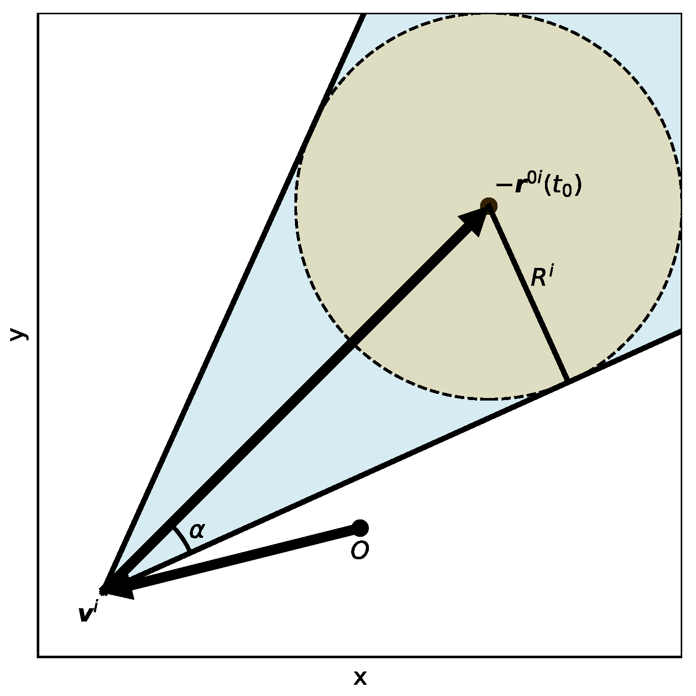
Figure 2.
Illustration of Equivalent Linear Velocity Obstacle. The debris moves with a varying velocity . At time , the debris reaches position with velocity , as indicated by the dashed circle . The dashed circle represents a virtual object that will reach at time with a constant velocity of . The ELVO of the satellite with respect to the i-th debris at time is defined by the VO of the satellite with respect to this virtual object.
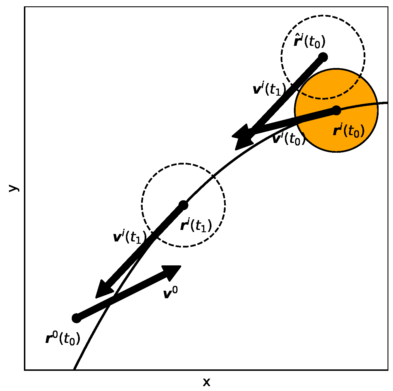
Figure 3.
Values of and with respect to .
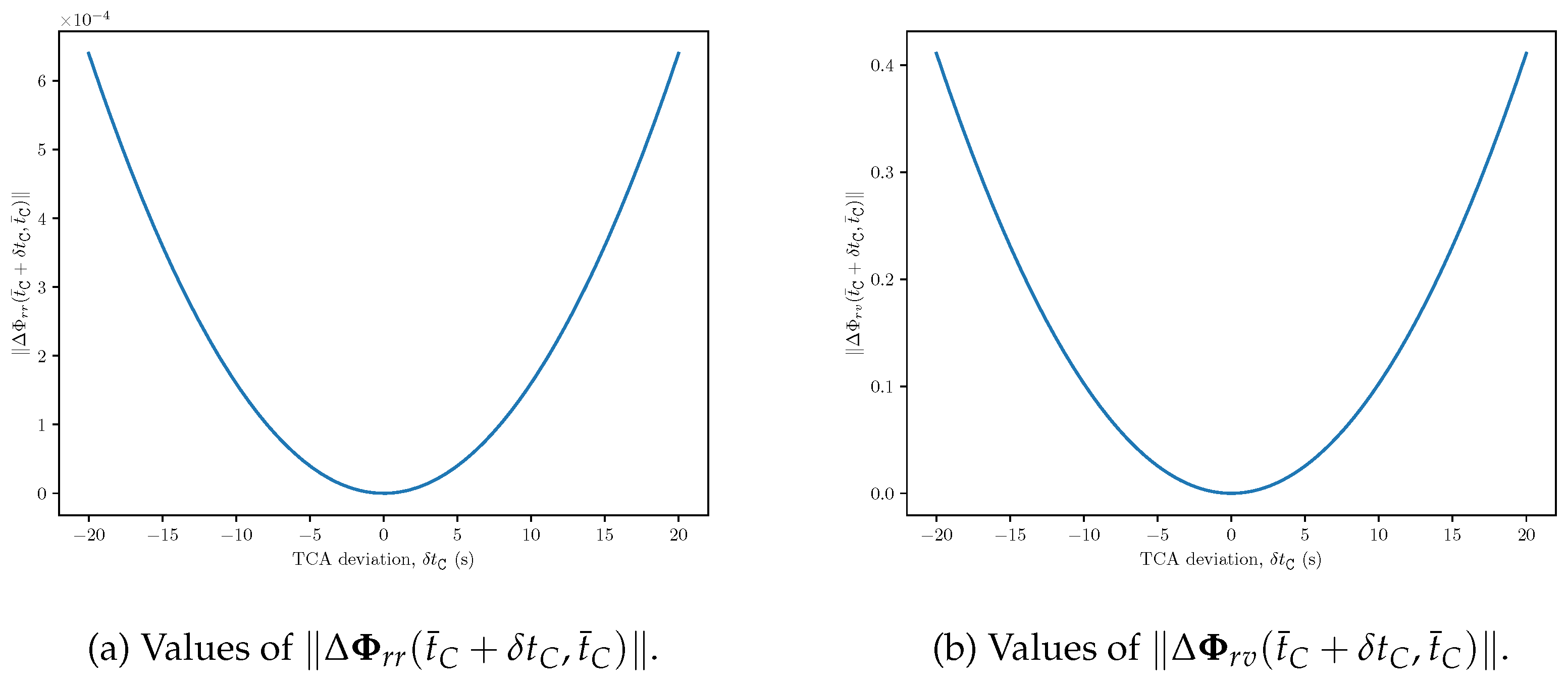
Figure 4.
Values of and .
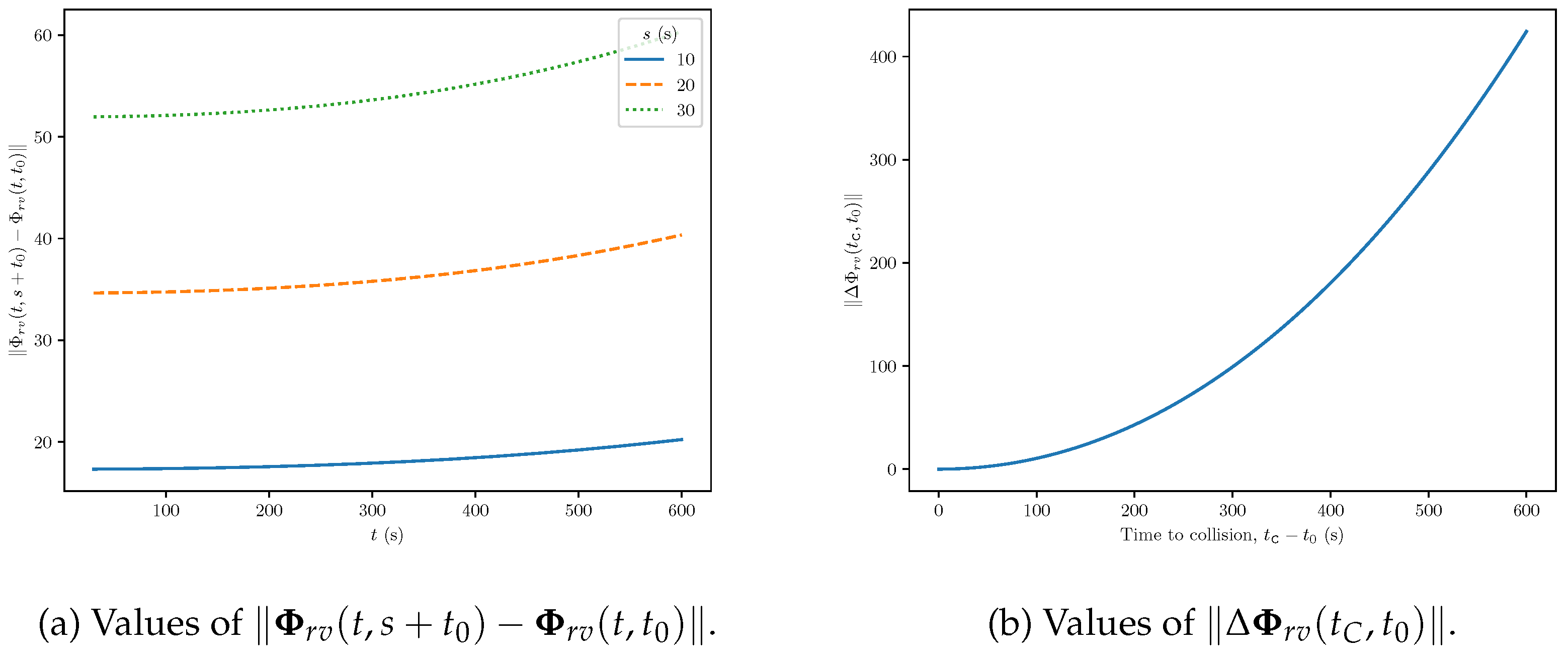
Figure 5.
Space debris collision avoidance procedure.
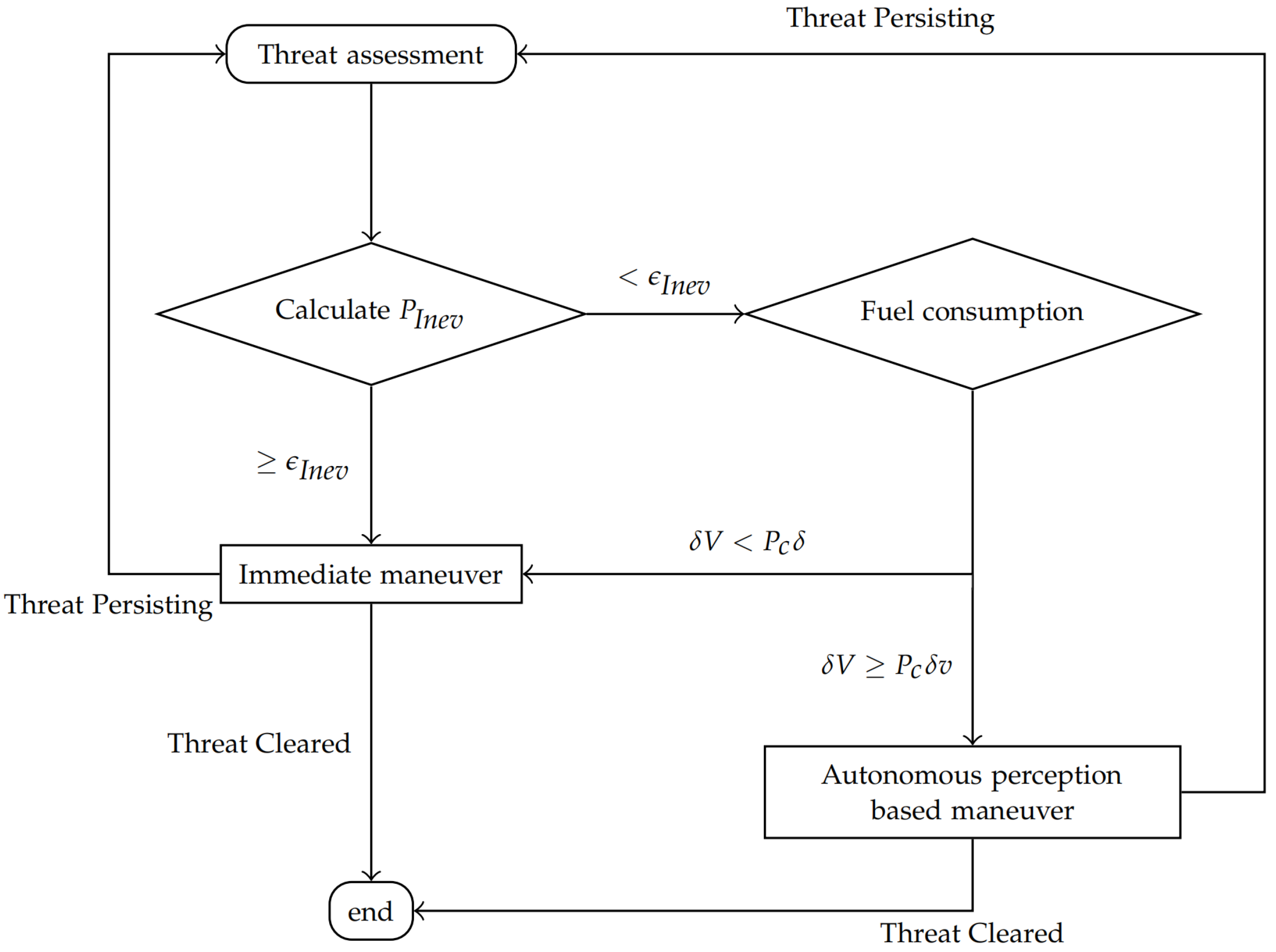
Figure 6.
Minimal distances between satellite and closest debris after maneuvers for Scenario 1.
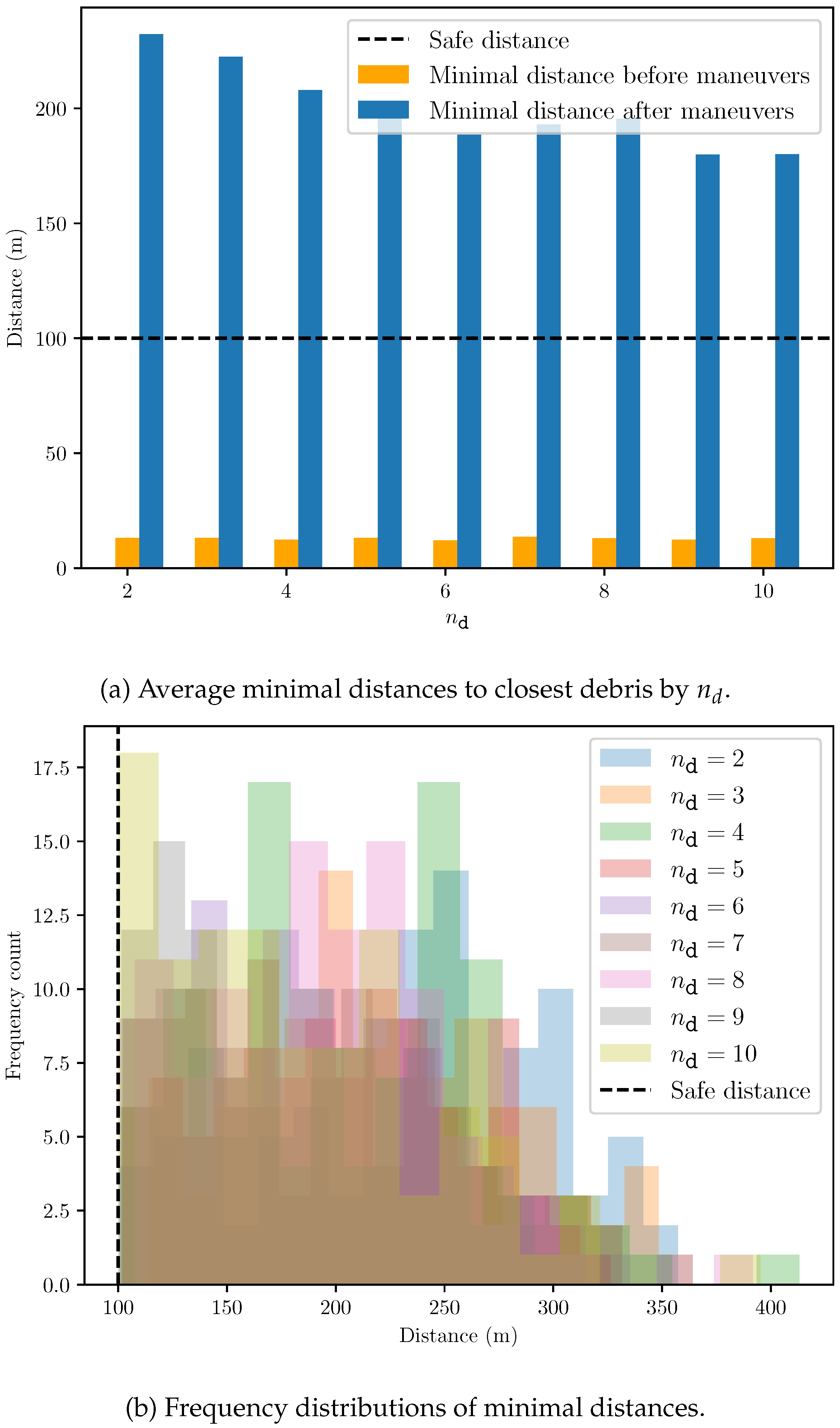
Figure 7.
Maneuver increments for Scenario 1.
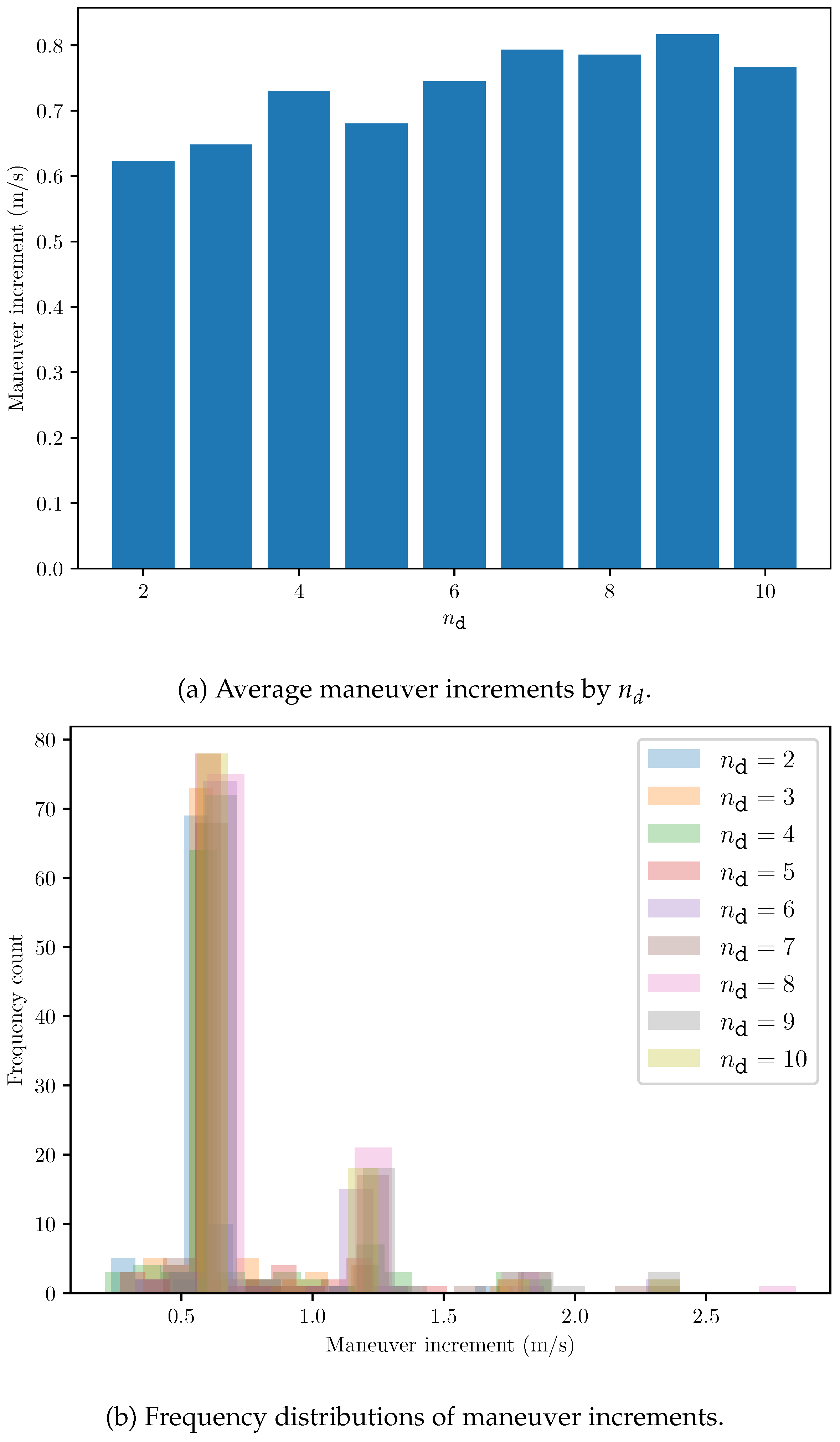
Figure 8.
Average running time of the algorithm. The time required for subsequent iterations is nearly zero. Both the propagation of the orbit and the solving of the ELVO problem are invoked once per programming iteration, i.e., for each .
Figure 8.
Average running time of the algorithm. The time required for subsequent iterations is nearly zero. Both the propagation of the orbit and the solving of the ELVO problem are invoked once per programming iteration, i.e., for each .
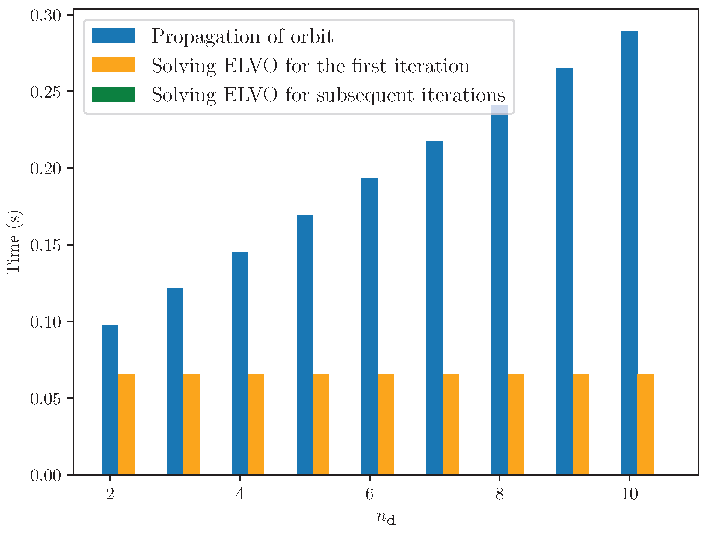

Table 1.
Initial orbital elements of reference satellite.
| Symbol | Description | Value |
|---|---|---|
| Semi-Major Axis | 7155.459 km | |
| Eccentricity | 1.174 | |
| Inclination | 1.292 rad | |
| RAAN | 0.301 rad | |
| Argument of Periapsis | 1.468 rad | |
| True Anomaly | 0.234 rad |
Table 2.
Satellite and algorithm parameters.
| Symbol | Description | Value |
|---|---|---|
| Maximal acceleration | 0.03 m/ | |
| max standard deviation of on-board position observation |
10 m | |
| max standard deviation of on-board velocity observation |
1 m/s | |
| T | Programming horizon | 20 s |
Table 3.
Parameters of debris in the satellite’s field of view, with relative positions and velocities in LVLH coordinate system. Simulations are generated by using data sampled from uniform distributions based on these parameters.
Table 3.
Parameters of debris in the satellite’s field of view, with relative positions and velocities in LVLH coordinate system. Simulations are generated by using data sampled from uniform distributions based on these parameters.
| Symbol | Description | Value |
|---|---|---|
| Number of debris pieces | 2 ∼ 10 | |
| safe distance | 100 m | |
| TCA | 400 ∼ 600 s | |
| TCA distance in x | 0 ∼ 500 m | |
| TCA distance in y | 0 ∼ 500 m | |
| TCA distance in z | 0 ∼ 500 m | |
| TCA velocity in x | 0 ∼ 50 m/s | |
| TCA velocity in y | 0 ∼ 100 m/s | |
| TCA velocity in z | 0 ∼ 100 m/s |
Table 4.
State of high-speed collision debris at TCA, with relative positions and velocities in LVLH coordinate system. The debris is far from the satellite at the initial time, outside its field of view.
Table 4.
State of high-speed collision debris at TCA, with relative positions and velocities in LVLH coordinate system. The debris is far from the satellite at the initial time, outside its field of view.
| Symbol | Description | Value |
|---|---|---|
| - | safe distance given by ground-based prediction |
8 km |
| TCA | 3600 s | |
| TCA distance in x | 0 m | |
| TCA distance in y | 0 m | |
| TCA distance in z | 0 m | |
| TCA velocity in x | 0 km/s | |
| TCA velocity in y | -7.440 km/s | |
| TCA velocity in z | -7.440 km/s |
Table 5.
Initial orbital elements of high-speed collision debris.
| Symbol | Description | Value |
|---|---|---|
| Initial Semi-Major Axis | 7168.867 km | |
| Initial Eccentricity | 2.990 | |
| Initial Inclination | 0.874 rad | |
| Initial RAAN | 2.115 rad | |
| Initial Argument of Periapsis | 0.833 rad | |
| Initial True Anomaly | -0.235 rad |
Table 6.
Parameters of planned avoidance orbit for impulse maneuver.
| Symbol | Description | Value |
|---|---|---|
| Maneuver increment | 0.82 m/s | |
| Target Semi-Major Axis | 7157.034 km | |
| Target Eccentricity | 1.39 | |
| Target Inclination | 1.292 rad | |
| Target RAAN | 0.301 rad | |
| Target Argument of Periapsis | 1.504 rad | |
| Target True Anomaly | 0.197 rad |
Table 7.
Orbital elements comparison for Scenario 2.
| Elements | Avoidance orbit (impulse) |
Reference orbit (no maneuver) |
Actual orbit (ELVO-based) |
|---|---|---|---|
| a (km) | 7164.859 | 7163.280 | 7165.757 |
| e | 2.733 | 2.524 | 2.850 |
| i (rad) | 1.292 | 1.292 | 1.292 |
| (rad) | 0.301 | 0.301 | 0.301 |
| (rad) | 1.399 | 1.373 | 1.414 |
| (rad) | 0.931 | 0.956 | 0.914 |
Disclaimer/Publisher’s Note: The statements, opinions and data contained in all publications are solely those of the individual author(s) and contributor(s) and not of MDPI and/or the editor(s). MDPI and/or the editor(s) disclaim responsibility for any injury to people or property resulting from any ideas, methods, instructions or products referred to in the content. |
© 2025 by the authors. Licensee MDPI, Basel, Switzerland. This article is an open access article distributed under the terms and conditions of the Creative Commons Attribution (CC BY) license (http://creativecommons.org/licenses/by/4.0/).
Copyright: This open access article is published under a Creative Commons CC BY 4.0 license, which permit the free download, distribution, and reuse, provided that the author and preprint are cited in any reuse.


