
Submitted:
24 March 2025
Posted:
25 March 2025
You are already at the latest version
Abstract
This study explores the growing application of 3D remote sensing in geohazard studies, particularly for rock slope monitoring. It highlights Street View Imagery (SVI) as a cost-effective alternative to traditional methods like UAVs. By comparing 3D point clouds generated from SVI data over time, researchers can track rockfall progression and quantify retreat volume. A case study in Koto Panjang cliff, Indonesia, demonstrates this approach. Utilizing seven years of SVI data, the study reveals a total rockfall retreat of 5,270 m3, with an average retreat rate of 7.53 m3/year. Structural analysis identified six major discontinuity sets and confirmed inherent instability within the rock mass. Kinematic simulations using SVI-derived data further assessed rockfall trajectories and potential impact zones. Results indicate that 40 % of simulated rockfall deposits accumulated near existing roads, with significant differences in distribution based on scree slope angles. This emphasizes the role of scree slope in influencing rockfall propagation. In conclusion, SVI presents a valuable tool for 3D point cloud reconstruction and rockfall hazard assessment, particularly in areas lacking historical data. The study showcases the effectiveness of using SVI in quantifying rockfall volume and identifying critical areas for mitigation strategies, highlighting the importance of scree slope angle in managing rockfall hazard.
Keywords:
Rockfall
; SVI
; Indonesia
1. Introduction
Geohazard investigations increasingly rely on three-dimensional remote sensing techniques, as they can effectively capture the shape and changes in natural hazards such as mass movements, lava flows, and debris flows by comparing 3-D point clouds acquired at different times [1]. These techniques are particularly useful in quantifying the evolution of rock slopes, including rockfall rates and deformation before failure, through the use of lidar technology [2,3,4] and point clouds obtained from photogrammetric methods [5,6,7,8,9].
The process of investigating rockfall changes can utilise technologies such as LiDAR [10,11,12] UAV with Structure from Motion (SfM) [5,7,8,13]. Those two methods yield point clouds, which are characterised by x, y, and z coordinates that portray a subject by representing it through a series of points. Point clouds that can reach centimetres [2] to sub-centimetre [14] resolution (i.e., point spacing) possess the potential to delineate topography with high precision, depending on the quality of the acquisitions. Through the quantitative analysis and comparison of topographic information acquired at distinct points in time, it becomes feasible to discern and gauge modifications associated with terrestrial surface processes [6].
Street view imagery (SVI) services, which provide 360° panoramas from various roads, streets, and locations worldwide, constitute a significant portion of the vast array of online images [15]. Street view images can be accessed through several providers such as Google Maps/Google Earth Pro [16], Apple Maps, Mappilary, Karta View, Baidu Maps and Tencent Street View [15,17]. In most cases, panoramic imagery is acquired using a car mounted with multiple cameras, accompanied by various sensors, including lidar, though backpack-mounted cameras are also used for surveying narrow roads [18]. In this study, we utilised Google Street View (GSV) as our data services provider. Initially, GSV was primarily used in urban areas for virtual street navigation, but its use has since expanded to such as non-urban areas allowing to asses the rate slope hazard through imagery [19] and for detecting and quantifying volume changes due to rock failures [20].
This research aims to illustrate that 3-D models generated from street view images can not only aid the identification of changes in the landscape of rock slopes but also reveal the evolutionary patterns of a rock cliff throughout the documented year in a region where regular surveying and monitoring systems for rockfall hazards are not in place.
2. Geological and Geographical Setting
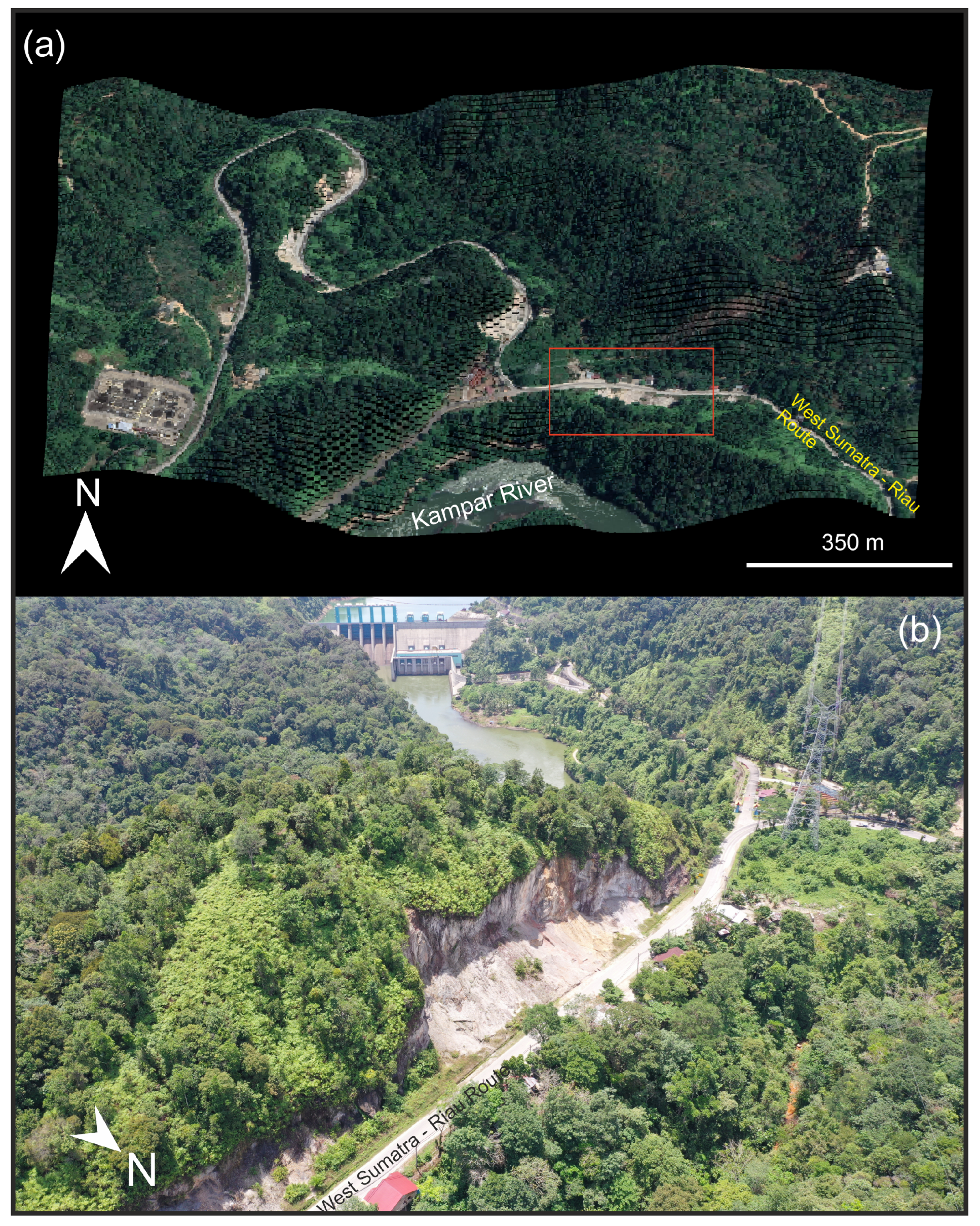
The study site is at KM 77 of the highway that connects the Riau and West Sumatra provinces, located within the Kampar Region of Riau Province, Sumatra Island, Indonesia (Figure 1). The studied rock cliff spans 170 metres laterally and stands 25 metres high, adjacent to the highway to the north and the Kampar River to the south. Three rockfall occurrences were documented in 2015, 2016, and 2019, obstructing the road. As a result, the economic route linking the Riau and West Sumatra provinces was adversely impacted (Figure 2).
The study site is part of the Bahorok Formation, composed of pebbly mudstone deposited in the Carboniferous – Early Permian [21]. This formation is mainly composed of non-bedded medium to coarse-grained breccioconglomeratic wackes [22], also The Bohorok Formation has generally been affected by low, slate-grade, and metamorphism [23]. Subordinate interbedded mudstones, siltstones, quartzose arenites, and lime-stones are also present. These pebbly mudstones have a silt to fine sand-grade matrix. Their clasts are angular to subrounded, and clast lithologies indicate a continental source; vein quartz, argillites, and arenites are dominant among less common limestones, mica schist, and granite. Gneiss, chloritic schist, greenish calcsilicate rocks, and possibly rhyolite also occur. Fresh angular microcline is prominent in thin section [24].
The main structural feature on the island of Sumatra is the Sumatra Fault System, which initiated in the Mid-Miocene. It was formed due to various superimposed tectonic events, including the widening of the Andaman Sea to the northwest of Sumatra and extension of the Sunda Strait to the southeast of Sumatra in ±11 Ma [25,26]. Additionally, it is also associated with the oblique subduction of the Indo-Australian plate beneath the Eurasian plate [27,28,29] at a rate of 7 cm/year [30]. The Sumatra Fault System is characterized by broad, sinusoidal faults with length on the order of ten kilometres [25]. Structures in the Kampar Regency mainly trend northwest-southeast and northeast-southwest. Fractures in the area comprise dextral strike-slip faults and normal faults. Also, it has an average persistence five fractures/ meter with mostly joint and vein [30].
Figure 1.
(a) Location of study site at KM 77 of the Riau-West Sumatra route in Kampar Regency, Riau, Indonesia;(b) Simplified geological situation of site which predominantly consist of metamorphic rock and northwest–southeast trending structures (modified after [31].
Figure 1.
(a) Location of study site at KM 77 of the Riau-West Sumatra route in Kampar Regency, Riau, Indonesia;(b) Simplified geological situation of site which predominantly consist of metamorphic rock and northwest–southeast trending structures (modified after [31].
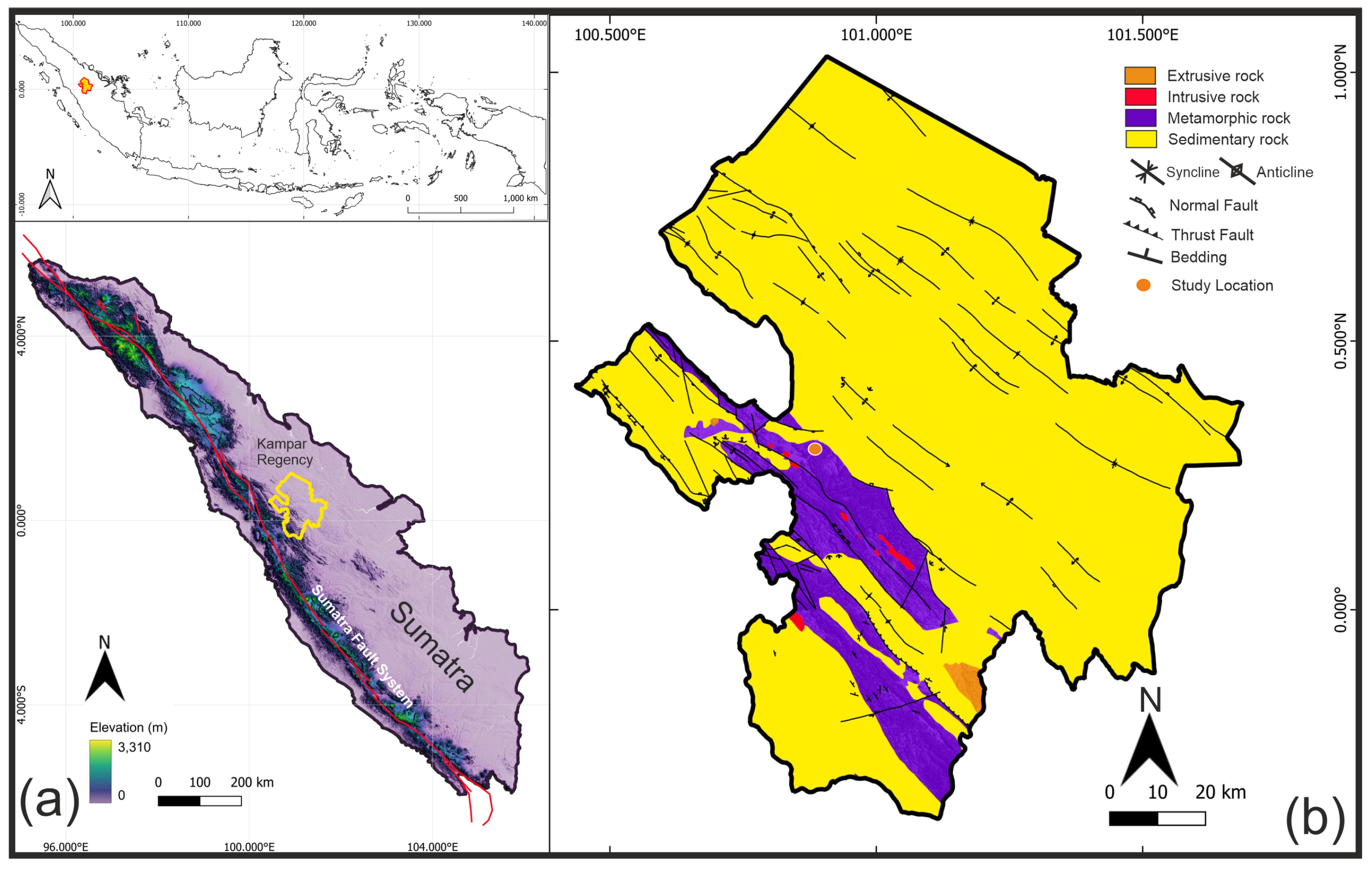
Figure 2.
(a) Oblique 3D view of aerial photo of the study area (modified from Google Earth) draped over a 8 m digital elevation model (DEM); (b) Oblique aerial photo of the study site, captured using a DJI Mavic Pro 2 UAV on July 2021.
Figure 2.
(a) Oblique 3D view of aerial photo of the study area (modified from Google Earth) draped over a 8 m digital elevation model (DEM); (b) Oblique aerial photo of the study site, captured using a DJI Mavic Pro 2 UAV on July 2021.
3. Methodology
3.1. Image Acquisition
Two types of images were used in this study, from which 3D point clouds of the studied rock face were generated: Google Street View panoramas (i.e., SVI) and images captured using a digital camera mounted on an Unmanned Aerial Vehicle (UAV) (Table 1). Street view panoramas were accessed and downloaded through the Google Street View Static API [32,33].The data has been historically by monthly accuracy collected by GSV from 2015 and continued to be captured yearly for up to seven consecutive years, ending in 2021.
In 2021, image acquisition was conducted using an unmanned aerial vehicle (UAV) equipped with a DJI Mavic 2 Pro. The UAV was fitted with a high-resolution camera capable of capturing images at 5472 x 3648 pixels, ensuring detailed and precise data collection. The point clouds generated from these UAV images were subsequently utilized for the calibration of point clouds derived from the SVI (Street View Imagery). This calibration process aimed to enhance the accuracy and consistency of the spatial data obtained from both sources.
3.2. Decomposing 360-degree SVI images
Panoramic SVI (i.e., equirectangular images; Figure 3a) were converted into perspective images (i.e., cube faces; Figure 3b), which are more suitable for further processing into 3D point clouds using a structure-from-motion (SfM) workflow. These high-quality 360-degree SVI (Table 1) were decomposed using a MATLAB script [34] that converted equirectangular images into six cube faces with a resolution of 3328 x 3328 pixels per cube face image (Figure 3). The process of deriving cube maps from equirectangular images followed the method of Bourke [35]:
The process begins by taking an equirectangular image as input. The width and height of this image are used to determine the size of the output cubic faces. If no specific output size is provided, a default size is calculated based on the width of the input image. Additionally, a vertical field of view (VFOV) is defined, determining how much of the spherical projection is visible in each face of the cube. By default, the VFOV is set to 90 o. Each face of the cube corresponds to a specific direction: front, right, back, left, top, and bottom (see Table 2). To define these directions, the function uses three angles: yaw, pitch, and roll. These angles describe how the cube face is oriented relative to the equirectangular image.
To project an equirectangular image onto the faces of a cube, the process begins by defining the point as as the top-left coordinate origin. This point serves as the reference for constructing the grid that will be mapped onto each cube face. The position of (in Figure 4a)is determined by the vertical field of view (vfof) and the dimensions of the target cube face, as mathematically formulated in Equation (1).
Here, and denote the width and height of each cubic face, respectively.
A scaling factor is derived to regulate the proportional spacing between grid points, as defined in Equation (2). This ensures the projected grid aligns precisely with the dimensions of the output cube face, preserving geometric accuracy during the mapping process.
where , , denote the x-, y-, and z-coordinates of the top-left reference point . For each cube face, a grid of spatial coordinates is generated, corresponding to pixel positions on the output face. This grid is initially constructed as a 2D array but is flattened into a sequential list of points to streamline computational processing. The initial coordinates are then transformed using and to , ensuring precise alignment between the grid and the equirectangular image. This transformation process is mathematically defined in the equations below:
where , , denote the scaling factors for the x-, y-, and z-axis components, respectively. The vectors , represent horizontal and vertical coordinate vectors of the grid. The initial 3D positions of the grid points, denoted as are computed by combining the base coordinates of the reference point and the scaled grid .
Since each cube face requires a distinct spatial orientation, rotation matrices are applied to achieve alignment. Equation (4) defines the composite transformation matrix for each face, constructed from Euler-angle rotations: (pitch), (yaw), (roll). This matrix rotates the grid points to match the target orientation of the cube face, ensuring seamless correspondence with the equirectangular projection.
The transformation matrix for each cube face is computed as the product of Euler-angle rotation matrices:
Then, The transformed 3D coordinates (see in Figure 4b), is achieved by applying T to the initial points :
After transformation, the points are repositioned in 3D space and decomposed into their cartesian components , , and . These components correspond to positions on the unit sphere represented by the equirectangular image.
The next step converts the 3D Cartesian coordinates to spherical coordinates, as defined by Equations (6) and (7). Here, each point is parameterized by two angles: the azimuth , which measures the horizontal direction around the sphere (left/right), and the , which measures the vertical direction above/below the equatorial plane (up/down).
These angles are then mapped to pixel coordinates in the equirectangular image. The mapping ensures that each point on the cube face corresponds to the correct location in the equirectangular image as following Equation (8) and (9):
where (, ) represent new horizontal and vertical pixel coordinate for cube face, and (,) denote the width and height of the equirectangular image in pixels. The azimuth angle , which spans , defines the horizontal position around the sphere, while the elevation angle , bounded between and , determines the vertical position relative to the equatorial plane. The scaling terms and normalize the angular ranges to the pixel dimensions of the output image.
After all cube-face images were generated, geospatial coordinates were embedded into the images using the ExifTool library [36].
3.3. Data Processing
3.3.1. Dense Points Cloud Model Generation
The process for image datasets of GSV in Kotopanjang is only three out of six image cubes, which represent part of the road and rock cliff. All the selected photographs were processed using Agisoft Metashape Professional (version 1.5.4) SfM-MVS (Multi-View Stereo) software [37]. Graber and Santi (2023) [6] explain the general process of creating 3D point clouds from images using Agisoft Metashape, which involves initial photo screening and importing, photo alignment and tie point selection, trimming of the sparse point cloud, optimization of the camera alignment, and creation of a dense, high-quality point cloud.
3.3.2. Georeferencing and Registration of 3D Model
Five point clouds generated from GSV images and one point clouds generated from UAV images were imported into the CloudCompare (version 2.12 alpha) software package for alignment and analysis. These 3D point clouds were aligned (i.e., co-registered) with a reference point cloud extracted from the national Digital Elevation Model (DEMNAS), which has a resolution of 8 meters per pixel. Preliminary alignment (i.e., coarse alignment) was performed by choosing a minimum of three pairs of points based on their features from the entire 3D point cloud.
Alignment of the point clouds was further improved using the Iterative Closest Point (ICP) algorithm [38], which minimised the root mean square error (RMSE) between the point clouds. Before applying the ICP technique, we marked two areas which were considered to be stable. The stabilisation of the remaining sections of the datasets, initially considered unstable, was achieved using the transformation matrix derived from the first step. The Poisson Surface Reconstruction algorithm [39] was then employed to produce a 3D mesh [39].
3.3.3. Change Detection of Point Clouds
We used the M3C2 plugin [40] within CloudCompare [41] to detect change between the point clouds. The cylindrical neighbourhoods were oriented using the normal vectors obtained during the SfM processing instead of creating new ones. All of the points in point cloud (01/2019; Figure 6), following down sampling and cleaning in the pre-processing steps, served as ’core points’ where the M3C2 calculation was carried out. Multiple neighbourhood sizes (representing the cylinder’s diameter) were applied for each change detection interval to ensure the detection of both small and large changes. For the point clouds, we used neighbourhood diameters of 0.3, 0.5, and 1.0 m. For every set of M3C2 distances, an empirical limit of detection (LOD) was determined by fitting a normal distribution to the M3C2 distance histogram. This process involved minimizing the sum of squared errors between the distance histogram and the normal distribution model. The empirical LOD was defined as the range within ±2 standard deviations from the mean M3C2 distance. M3C2 distances were computed between the initial and final scans for each slope to identify potential rock-falls throughout the monitoring campaign. After assessing the changes, alterations exceeding the empirical LOD were manually inspected to distinguish rockfalls from other factors such as erosion, missed vegetation, photogrammetric noise, or registration error. To confirm each rockfall sources and to bracket the timing of each rockfall events as closely as possible, we reviewed all the photo datasets for the relevant locations where changes occurred[40].
3.3.4. Rockfall Clustering and Volume Calculation
In the process of validating each rockfall occurrence and pinpointing their timing with precision, the photo datasets relating to the specific areas where the changes took place were carefully analysed. In cases where changes were unclear, the photo datasets were used to confirm their correlation with rockfall incidents. The examination of change plots and RGB photos served the purpose of pinpointing the locations linked to rockfalls [12]. Following that, we manually defined and separated the clusters of points linked to rockfall events. The rockfall volume calculation was conducted using the 3D alpha-shape method, as per the guidelines proposed by [7,42].
3.3.5. Structural Measurement and Kinematic Analysis
By utilizing georeferenced 3D point cloud data acquired through SfM photogrammetry and Coltop3D software [43], a 3D shaded, coloured relief map was generated, with colours corresponding to the rock cliff orientation (slope aspect and angle) (Figure 5). These point clouds enabled topographic and structural analyses, which are critical to the study of rock slopes that are remote or difficult to access, making traditional field investigations challenging. To gain a better understanding of how discontinuities contribute to progressive slope failure, it is essential to determine the discontinuity sets involved in past events. Using the point clouds, we were able to identify the discontinuity sets associated with rock slope instability. Six primary joint sets (J1 to J6) were identified in the Coltop3D software. The point cloud of each discontinuity set was imported into CloudCompare, where it was compared with the locations of rockfall sources (interpreted from the point cloud of the rock cliff) [44]. This method allowed us to determine the number of rockfalls each joint set had been involved in.
Kinematic analysis from also provided by examining the potential movement of rock blocks on point clouds which performs using DIPS and StnParabel software. This analytical approach is particularly done by identifying types of block failures, such as sliding, toppling, or falling, which can occur due to the orientation of geological discontinuities, including joints and faults.
3.3.6. Precipitation Analysis
In analyzing precipitation data, two data sources were used, weather station data from 2018 - 2021, and NASA Global Precipitation Measurement (GPM) data using The Integrated Multi-satellite Retrievals for GPM (IMERG) algorithm to estimate precipitation over the majority of the Earth’s surface [45]. The analysis is done by calculating the Antecedent precipitation index (API)[46] against daily weather precipitation data, combined with temperature data plots. As for the GPM data, we selected the IMERG precipitation Half Hourly 0.1 degree x 0.1 degree V06 and IMERG precipitation day 0.1 degree x 0.1 degree V06 product which provides more accurate precipitation information across Global Precipitation Climatology Centre (GPCC)-gauged regions compared to the near real-time products [45]. The data was selected based on rockfall events that occurred on November 13, 2016. This IMERG plot data is taken on rockfall events that occurred in 2016 because weather station data has not covered data before 2018. Data processing is done by extracting. hdf5 which can be accessed on https://www.earthdata.nasa.gov/ and taking daily and 24-hour data every half hour. The data is calculated cumulatively daily and plotted by overlaying the study location point.
3.3.7. Trajectography Analysis
Simulation of rockfall trajectories and impacts was performed with stnParabel [47], using the point cloud as topographic input. This algorithm takes into account the size and shape of the falling rock, the roughness of the terrain, the gravitational potential energy of the rock, air resistance, and frictional forces between the rock and terrain. For this simulation, the point cloud is used to represent the terrain over which the rockfall is simulated. For the data preparation, we used a set of data points in a 3D coordinate system that represents the surface of an object or terrain. In this case, the point cloud represents the terrain over which the rockfall is simulated. Detail of spacing point cloud is defined on how big the size of the rock. So smaller size of the rock will follow by the density of the point spacing between the point cloud [48]. We utilized kinematic analysis for source identification and integrated the results into the provided instruction website for detailed steps [48].
4. Results
4.1. Structural Interpretation
This scarp area shows a slope face oriented on average at , with a dip slope up to . The scarp has a length of 165 m, 50 m in height, with six main discontinuity sets (J1 to J6) that identified from point cloud data and direct field measurements Table 3. J1 and J3 stand out as pervasive joint sets that are present almost along the entire outcrop. These sets are similarly oriented to regional fracture zones (Figure 5).
Based on the collected discontinuity and slope orientation data from the rockfall source zone. Although the orientation of discontinuity sets may slightly vary at different sections, a total of two dominant discontinuity sets (J1 and J3) were identified; , (Figure 5). The friction angle of discontinuities in the rockfall source zone was calculated to be . Based on the kinematic analyses conducted for the rockfall source zone, it was determined that the most common discontinuity-controlled failure type on the source zone is wedge and block toppling failure (Figure 5). This dominant discontinuity is attributable to its alignment with a regional fracture zone.
4.2. Comparison of Point Cloud Data
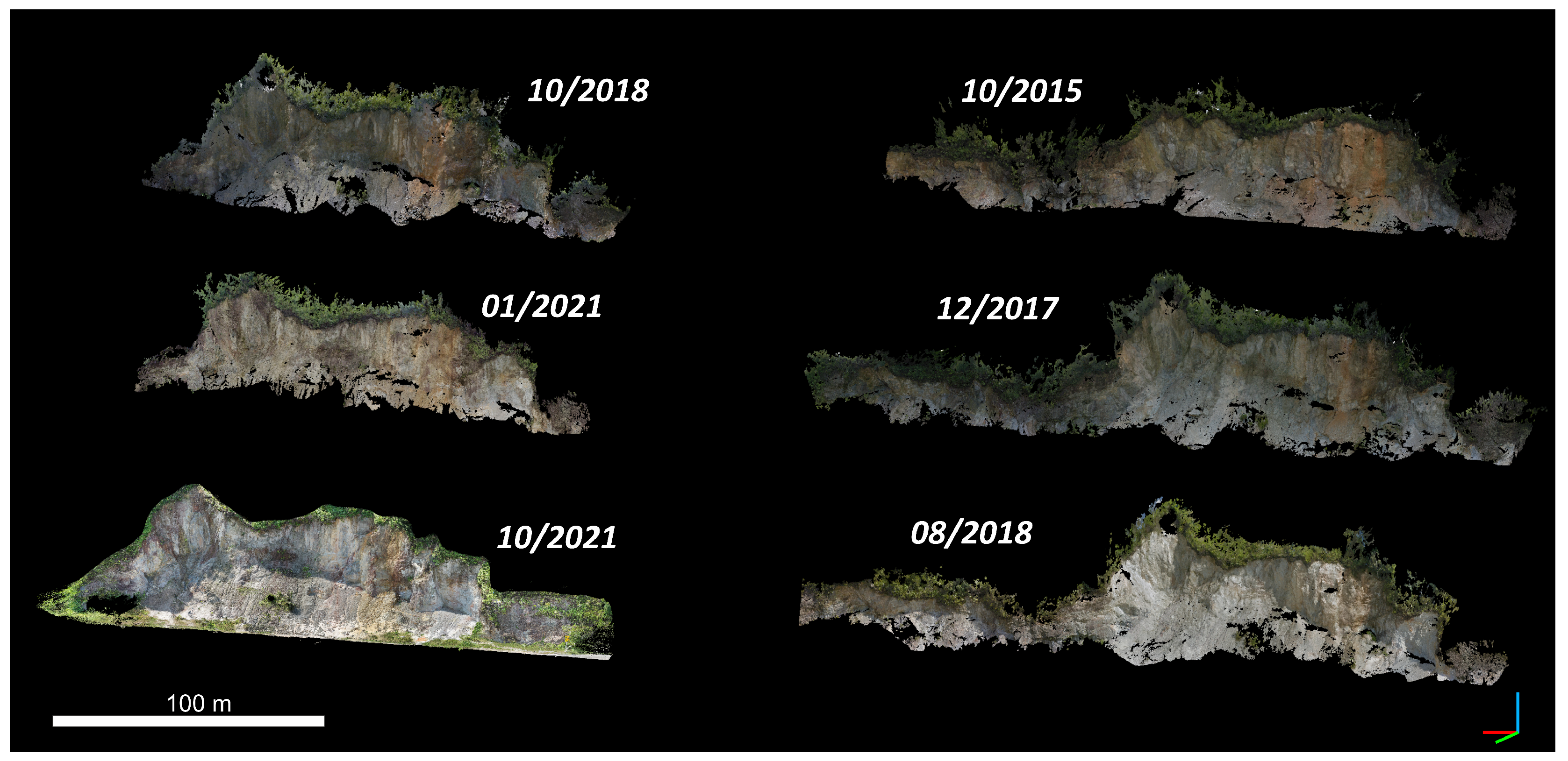
Based on the results of SVI and UAV data processing using Agisoft software, seven point clouds can each be processed and compared. The result covered all the cliff scarp in the area, only SVI from 01/2019 that have missing section of the scarp (Figure 6).
The topography of the studied rock cliff appears to have changed significantly between 2015 and 2021 due to mining and rock collapse (Figure 7). By comparing the 3D point clouds from these years, 27 rockfall source areas are identified as source of rockfall, with volumes ranging from 8 to 1774 , have been identified. Between October 2015 and December 2017, 11 rockfalls occurred, followed by 7 rockfalls between December 2017 and October 2018 and 10 rockfalls between October 2018 and October 2021 (Figure 7). The cumulative rockfall volume from 2015 to 2021 was approximately 5.27 × m. On average, 3.85 rockfall events occurred annually, resulting in a total volume change of 7.53 from 2015 to 2021.
Figure 6.
Result of SfM for 7 years of SVI data from 2015 – 2021. The 3D point clouds from 10/2015 to 01/2021 are resulted using images from SVI and 10/2021 are result from UAV acquisitions.
Figure 6.
Result of SfM for 7 years of SVI data from 2015 – 2021. The 3D point clouds from 10/2015 to 01/2021 are resulted using images from SVI and 10/2021 are result from UAV acquisitions.
The volume-frequency (V-F) relationship for rockfalls and rock fall sources volumes is distributed according to a power law [49]. Before 2015, no data were noted and recorded. This might make our estimates more cautious, leading to a calculated return period for rock failure that may differ from its actual frequency but align with the power law pattern. The relationship differs if we consider only the events from 2015 to 2021 or if we include two large events from 2016 and one from 2018. The corresponding power law fittings for 27 blocks retreat are as follows: = 22.43 obtained using least squares linear regression. In this case, the minimum, or cut off, volume () of the power law fitting is set as 5.25 (Figure 8).
Concluding that the scaling exponent b, crucial for assessing the frequency of rock failure events, is more significantly influenced by the maximum recorded rock failure volume in the historical inventory than by the minimum volume, and it achieved this by analysing both types of volumes through regression and using the scaling exponent b from published references [6,50]. The insufficient representation of large rock failure events in fitting the power-law tail profoundly impacts the ability to predict the frequency of future, more significant events. This underscores the importance of considering the maximum rock failure magnitude in the inventory to pre-vent unrealistic extrapolation and to accurately determine the frequency or return period of larger failure events.
4.3. Precipitation Analysis
A detailed analysis of GPM-IMERG data on 1-day before the event (13/10/2016) on reveals a surge in rainfall intensity starting on 15:00 until 20:00, with values ranging from 32–36 mm/day, and lasted for 5 hours. This substantial rainfall peak stands out prominently amidst the overall rainfall distribution for the day, accumulating to a total of 220–240 mm/day (Figure 9a). Meanwhile, based on the climatological weather daily precipitation data, it shows the maximum API value of 189.33 mm and the lowest at 2.69 mm (Figure 9b). This indicates theres an increase in rainfall happen just before the rockfall event occured at that time.
4.4. Trajectography Results
Upon analyzing the processed kinematic analysis data, we identified 1542 potential sources. Subsequent simulations parameter were conducted using a rolling friction algorithm for impact model and a volume size of 1 x 1 , with 100 simulations performed for each point source as detail parameter shown in (Table 4) and in 3D view perspective (Figure 10a).
The simulation results of the simulated from rockfall deposits primarily which approximately 40% accumulated at locations where roads and infrastructure were present, generating translational kinetic energy impacts with an average value of 52 and a maximum value of 321 . Additionally, the average energy line exhibited a value of (Figure 10d).
Particularly noteworthy is the differential distribution of deposited rockfall across sectors with scree slopes exceeding and those with slopes below . This distinction underscores the significant impact of scree slope on rockfall trajectories. As evident from (Figure 10b), the eastern sector consistently exhibits a more extended trajectory compared to the western sector, demonstrating the pronounced influence of scree angle on rockfall distribution. This is also shown by the roughness in the eastern sector which is higher due to to active scree slope accumulated from rockfall events while the western sector has already excavated and less accumulated rockfall which tends to be more flat.
5. Discussion
5.1. Volume Calculation
While the identified discontinuity sets and orientations matched field observations, normal spacing remained unknown due to inaccessible rock faces. Utilizing 3D point cloud data and existing methods allowed for an objective estimation of normal spacing and, consequently, the detached block’s average volume. Factoring in this size provides more realistic travel distances and energies as the fallen block fragments along existing discontinuities[51].
Decomposing images from street view imagery could provide a solution in order to provide historical topography relief condition although it gives a lower detail resolutions compared with recent technologies using UAV and LiDAR. Since our result also related to the volume calculation which carried out solely uses the ICP (iterative closest point) method with UAV data that has been calibrated and georeferenced with DEM data. It is still necessary to pay attention to the volume of the comparison results between point clouds that can provide a large enough standard deviation on the accuracy of the data used in the calculation of the magnitude frequency relationship graph [6,52].
From the detected block release using detection of point cloud maximum detected is around 1.7 x and the smallest block is around 5.25 , this result giving some varianve between total number of rockfall and rock mining done by the locals. also this result is still insufficient representation of large rock failure events in fitting the power-law tail profoundly impacts the ability to predict the frequency of future, more significant events [6]. This underscores the importance of considering the maximum rock failure magnitude in the inventory especially on the ground which has became block fragment to prevent unrealistic extrapolation and to accurately determine the frequency or return period of larger failure events. However since there are no comparison related to previous data result, so inventory plays an important role for predicting a future failure rockfall events.
5.2. Simulation Accuracy
Block size significantly impacts the outcomes of 3D rockfall simulations, influencing both trajectories and energy loss [52]. While the average size can be estimated from past rockfall deposits, this method is often impractical due to the immense number of blocks involved. Additionally, fragmentation during the rockfall itself can render such measurements inaccurate[51].
Predicting rockfall trajectories is complex due to inherent uncertainties in both the rockfall process itself and the computer modeling techniques used. These uncertainties can be addressed by incorporating probability models for factors like source location, soil properties, initial conditions, and terrain features within the rockfall process. Our findings indicate a potential 40% probability of road closures, primarily correlated with historical rockfall events. Although we lack precise data on the location of past rockfalls, as these are often promptly addressed by road engineers, our simulations suggest a continued risk of future rockfall incidents impacting the roadway.
Similarly, uncertainties in numerical modeling can be mitigated by applying probabilistic models to simulate rockfall dynamics. While stnparabel software offers a probabilistic component encompassing most parameters [48], it still needs to explore more on rock fragmentation modeling capabilities. This probabilistic approach presents a valuable alternative, particularly in emergency situations where data is scarce.
6. Conclusions
In this paper, we provide the use of street view imagery as an alternative solution to be able to reconstruct 3D point clouds and provide comparison for evolution retreat of rockwall with decomposing the images rather than processed directly from the panorama images. Although, the detail of point cloud resulted less than UAV, however, it can give the best picture if there is no historical data or report at all related to rockfall events. According to cumulative volume comparison between 2015 - 2021 data shows 5.27 × has been fallen or near the road. This further reinforces that there is a possibility of periodic events that make this area a priority to be monitored. The results of the structural kinematic analysis show the possibility of wedge and direct toppling failures holding an important influence in the occurrence of failures that occur in the rock wall. From the comparison of scree in both east and west sectors, it shows that lowering the scree angle gives the possibility of slowing down the trajectory.
Author Contributions
Conceptualization, T.C., M.J., Y.Y.; methodology, T.C.; field investigation, T.C., Y.Y. and L.F; re-sources, H.W.; data curation, T.C.; writing—original draft preparation, T.C., Y.Y., L.F.; writ-ing—review and editing, T.C., Y.Y., M.J, A.S., L.F., M.D. ; visualization, T.C.; supervision, M.J, A.S., M.D.; funding acquisition, T.C. M.J,. All authors have read and agreed to the published version of the manuscript.
Funding
This research was funded by the Beasiswa Unggulan Dosen Indonesia LPDP of Ministry of Finance Indonesia (NO. 201905220214428).
Data Availability Statement
The data presented in this study are available upon the request from the corresponding author.
Acknowledgments
The authors gratefully acknowledge the support from LPDP Indonesia and the Department of Geological Engineering, Universitas Islam Riau. The entire team of the RISK Group of the University of Lausanne are also thanked for providing help, support, and feedback.
Conflicts of Interest
The authors declare no conflicts of interest.
References
- Voumard, J.; Abellán, A.; Nicolet, P.; Penna, I.; Chanut, M.A.; Derron, M.H.; Jaboyedoff, M. Using street view imagery for 3-D survey of rock slope failures. Natural Hazards and Earth System Sciences 2017, 17, 2093–2107. [Google Scholar] [CrossRef]
- Kromer, R.A.; Hutchinson, D.J.; Lato, M.J.; Gauthier, D.; Edwards, T. Identifying rock slope failure precursors using LiDAR for transportation corridor hazard management. Engineering Geology 2015, 195, 93–103. [Google Scholar] [CrossRef]
- Oppikofer, T.; Jaboyedoff, M.; Blikra, L.; Derron, M.H.; Metzger, R. Characterization and monitoring of the Åknes rockslide using terrestrial laser scanning. Natural Hazards and Earth System Sciences 2009, 9, 1003–1019. [Google Scholar] [CrossRef]
- Rosser, N.J.; Petley, D.; Lim, M.; Dunning, S.; Allison, R. Terrestrial laser scanning for monitoring the process of hard rock coastal cliff erosion. Quarterly Journal of Engineering Geology and Hydrogeology 2005, 38, 363–375. [Google Scholar] [CrossRef]
- Fernandez-Hernández, M.; Paredes, C.; Castedo, R.; Llorente, M.; de la Vega-Panizo, R. Rockfall detachment susceptibility map in El Hierro Island, Canary Islands, Spain. Natural hazards 2012, 64, 1247–1271. [Google Scholar] [CrossRef]
- Graber, A.; Santi, P. UAV-photogrammetry rockfall monitoring of natural slopes in Glenwood Canyon, CO, USA: Background activity and post-wildfire impacts. Landslides 2023, 20, 229–248. [Google Scholar] [CrossRef]
- Guerin, A.; Abellán, A.; Matasci, B.; Jaboyedoff, M.; Derron, M.H.; Ravanel, L. Brief communication: 3-D reconstruction of a collapsed rock pillar from Web-retrieved images and terrestrial lidar data–the 2005 event of the west face of the Drus (Mont Blanc massif). Natural Hazards and Earth System Sciences 2017, 17, 1207–1220. [Google Scholar] [CrossRef]
- Lucieer, A.; Jong, S.M.d.; Turner, D. Mapping landslide displacements using Structure from Motion (SfM) and image correlation of multi-temporal UAV photography. Progress in physical geography 2014, 38, 97–116. [Google Scholar] [CrossRef]
- Walstra, J.; Chandler, J.; Dixon, N.; Dijkstra, T. Aerial photography and digital photogrammetry for landslide monitoring. Geological Society, London, Special Publications 2007, 283, 53–63. [Google Scholar] [CrossRef]
- Jaboyedoff, M.; Oppikofer, T.; Abellán, A.; Derron, M.H.; Loye, A.; Metzger, R.; Pedrazzini, A. Use of LIDAR in landslide investigations: a review. Natural hazards 2012, 61, 5–28. [Google Scholar] [CrossRef]
- Lan, H.; Martin, C.D.; Zhou, C.; Lim, C.H. Rockfall hazard analysis using LiDAR and spatial modeling. Geomorphology 2010, 118, 213–223. [Google Scholar] [CrossRef]
- Tonini, M.; Abellan, A. Rockfall detection from terrestrial LiDAR point clouds: A clustering approach using R. Journal of Spatial Information Science 2014, pp. 95–110. [CrossRef]
- Vanneschi, C.; Camillo, M.D.; Aiello, E.; Bonciani, F.; Salvini, R. SFM-MVS photogrammetry for rockfall analysis and hazard assessment along the ancient roman via Flaminia road at the Furlo gorge (Italy). ISPRS International Journal of Geo-Information 2019, 8. [Google Scholar] [CrossRef]
- Williams, J.G.; Rosser, N.J.; Hardy, R.J.; Brain, M.J.; Afana, A.A. Optimising 4-D surface change detection: an approach for capturing rockfall magnitude–frequency. Earth Surface Dynamics 2018, 6, 101–119, Publisher: Copernicus GmbH. [Google Scholar] [CrossRef]
- Li, Y.; Peng, L.; Wu, C.; Zhang, J. Street View Imagery (SVI) in the Built Environment: A Theoretical and Systematic Review. Buildings 2022, 12, 1167, 32 citations (Crossref) [2024-06-28]. [Google Scholar] [CrossRef]
- Google. Explore Street View and add your own 360 images to Google Maps.
- Biljecki, F.; Ito, K. Street view imagery in urban analytics and GIS: A review. Landsc. Urban Plan. 2021, 215. [Google Scholar] [CrossRef]
- Anguelov, D.; Dulong, C.; Filip, D.; Frueh, C.; Lafon, S.; Lyon, R.; Ogale, A.; Vincent, L.; Weaver, J. Google Street View: Capturing the World at Street Level. Computer 2010, 43, 32–38. [Google Scholar] [CrossRef]
- William, S.; Yonathan, A. Using google earth and google street view to rate rock slope hazards. Environmental and Engineering Geoscience 2018, 24, 237–250. [Google Scholar] [CrossRef]
- Guerin, A.; Stock, G.M.; Radue, M.J.; Jaboyedoff, M.; Collins, B.D.; Matasci, B.; Avdievitch, N.; Derron, M.H. Quantifying 40 years of rockfall activity in Yosemite Valley with historical Structure-from-Motion photogrammetry and terrestrial laser scanning. Geomorphology (Amst.) 2020, 356, 107069, Publisher: Elsevier BV. [Google Scholar] [CrossRef]
- Cameron, N.R. The geological evolution of Northern Sumatra. In Proceedings of the Proc. Indon Petrol. Assoc., 9th Ann. Conv, Jakarta, 2018.
- Crowell, J.C. Origin of Pebbly Mudstones. GSA Bulletin 1957, 68, 993–1010. [Google Scholar] [CrossRef]
- Koesoemadinata, R.P. An Inroduction Into the Geology of Indonesia (General Inroduction and Part I Western Indonesia); Vol. 1, Ikatan Alumni Teknik Geologi ITB.
- Cameron, N.R. The stratigraphy of the Sihapas Formation in the Northwest of the Central Sumatra Basin. Indonesian Petroleum Association, Proceedings 12th annual convention 1983, I, 43–66.
- Curray, J.R. The Sunda Arc: A model for oblique plate convergence. Neth. J. Sea Res. 1989, 24, 131–140, Publisher: Elsevier BV. [Google Scholar] [CrossRef]
- Huchon, P.; Le Pichon, X. Sunda strait and central sumatra fault. Geology 1984, 12, 668–672. [Google Scholar] [CrossRef]
- Hamilton, W.B. Tectonics of the Indonesian region. Report 1078, USGS, 1979. [Google Scholar] [CrossRef]
- Katili, J.A. A review of the geotectonic theories and tectonic maps of Indonesia. Earth-Science Reviews 1971, 7, 143–163. [Google Scholar] [CrossRef]
- McCaffrey, R. The tectonic framework of the Sumatran subduction zone. Annu. Rev. Earth Planet. Sci. 2009, 37, 345–366. [Google Scholar] [CrossRef]
- Barber, A.J. The origin of the Woyla Terranes in Sumatra and the late Mesozoic evolution of the Sundaland margin. Journal of Asian Earth Sciences 2000, 18, 713–738. [Google Scholar] [CrossRef]
- Barber.; Crow. Sumatra: geology, resources and tectonic evolution (references). Tectonics 2005, 21, 1040. [CrossRef]
- Bruno, N.; Roncella, R. Accuracy assessment of 3d models generated from Google Street View imagery. ISPRS - Int. Arch. Photogramm. Remote Sens. Spat. Inf. Sci. 2019, XLII-2/W9, 181–188. [Google Scholar] [CrossRef]
- Yin, L.; Cheng, Q.; Wang, Z.; Shao, Z. `Big data’ for pedestrian volume: Exploring the use of Google Street View images for pedestrian counts. Appl. Geogr. 2015, 63, 337–345. [Google Scholar] [CrossRef]
- Phan, R. equi2cubic: MATLAB script that converts equirectangular images into six cube faces, 2015.
- Bourke, P. Converting to/from cubemaps, 2020.
- Harvey, P. ExifTool 10.11. Kingston, Ontario, Canada 2016.
- Agisoft. Agisoft Metashape User Manual-Professional Edition; Agisoft, 2022.
- Besl, P.J.; McKay, N.D. A method for registration of 3-D shapes. IEEE Trans. Pattern Anal. Mach. Intell. 1992, 14, 239–256, Publisher: Institute of Electrical and Electronics Engineers (IEEE). [Google Scholar] [CrossRef]
- Kazhdan, M.; Hoppe, H. Screened poisson surface reconstruction. ACM Trans. Graph. 2013, 32, 1–13, Publisher: Association for Computing Machinery (ACM). [Google Scholar] [CrossRef]
- Lague, D.; Brodu, N.; Leroux, J. Accurate 3D comparison of complex topography with terrestrial laser scanner: Application to the Rangitikei canyon (N-Z). ISPRS Journal of Photogrammetry and Remote Sensing 2013, 82, 10–26. [Google Scholar] [CrossRef]
- CloudCompare. CloudCompare 2.12 [GPL Software] 2022.
- van Veen, M.J. Building a Rockfall Database Using Remote Sensing : Techniques for Hazard Management in Canadian Rail Corridors. PhD thesis, Queen’s University, Kingston, Ontario, Canada, 2016.
- Jaboyedoff, M.; Metzger, R.; Oppikofer, T.; Couture, R.; Derron, M.H.; Locat, J.; Turmel, D. New insight techniques to analyze rock-slope relief using DEM and 3D-imaging cloud points: COLTOP-3D software. Proceedings of the 1st Canada-US Rock Mechanics Symposium - Rock Mechanics Meeting Society’s Challenges and Demands 2007, 1, 61–68. [Google Scholar] [CrossRef]
- Matasci, B.; Stock, G.M.; Jaboyedoff, M.; Carrea, D.; Collins, B.D.; Guérin, A.; Matasci, G.; Ravanel, L. Assessing rockfall susceptibility in steep and overhanging slopes using three-dimensional analysis of failure mechanisms. Landslides 2018, 15, 859–878, Publisher: Landslides ISBN: 1034601709. [Google Scholar] [CrossRef]
- Hufmann, G.J.; Stocker, E.F.; Bolvin, D.T.; Nelkin, E.J.; Tan, J. GPM IMERG Final Precipitation L3 Half Hourly 0.1 degree x 0.1 degree V06. NASA Goddard Earth Sciences Data and Information Services Center 2019.
- Fedora, M.; Beschta, R. Storm runoff simulation using an antecedent precipitation index (API) model. Journal of hydrology 1989, 112, 121–133, Publisher: Elsevier. [Google Scholar] [CrossRef]
- Noël, F.; Cloutier, C.; Jaboyedoff, M.; Locat, J. Impact-Detection Algorithm That Uses Point Clouds as Topographic Inputs for 3D Rockfall Simulations. Geosciences 2021, 11, 188, Publisher: MDPI AG. [Google Scholar] [CrossRef]
- Noel, F. stnParabel documentation, 2021.
- Graber, A. Power law models for rockfall frequency-magnitude distributions: review and identification of factors that influence the scaling exponent. Geomorphology 2022, 418. 12 citations (Crossref) [2024-07-08] Type: Review. [Google Scholar] [CrossRef]
- Hantz, D.; Corominas, J.; Crosta, G.B.; Jaboyedoff, M. Definitions and Concepts for Quantitative Rockfall Hazard and Risk Analysis. Geosciences 2021, 11, 158, Publisher: MDPI AG. [Google Scholar] [CrossRef]
- Corominas, J.; Mavrouli, O.; Ruiz-Carulla, R. Rockfall Occurrence and Fragmentation. In Proceedings of the Advancing Culture of Living with Landslides; Sassa, K.; Mikoš, M.; Yin, Y., Eds. Springer International Publishing, 2017, pp. 75–97. [CrossRef]
- Moos, C.; Bontognali, Z.; Dorren, L.; Jaboyedoff, M.; Hantz, D. Estimating rockfall and block volume scenarios based on a straightforward rockfall frequency model. Engineering Geology 2022, 309, 106828. [Google Scholar] [CrossRef]
Figure 3.
Example of (a) panoramic image (i.e., equirectangular image) that has been converted into (b) six cubic images (i.e., perspective images) (see Figure 4 and Table 2)
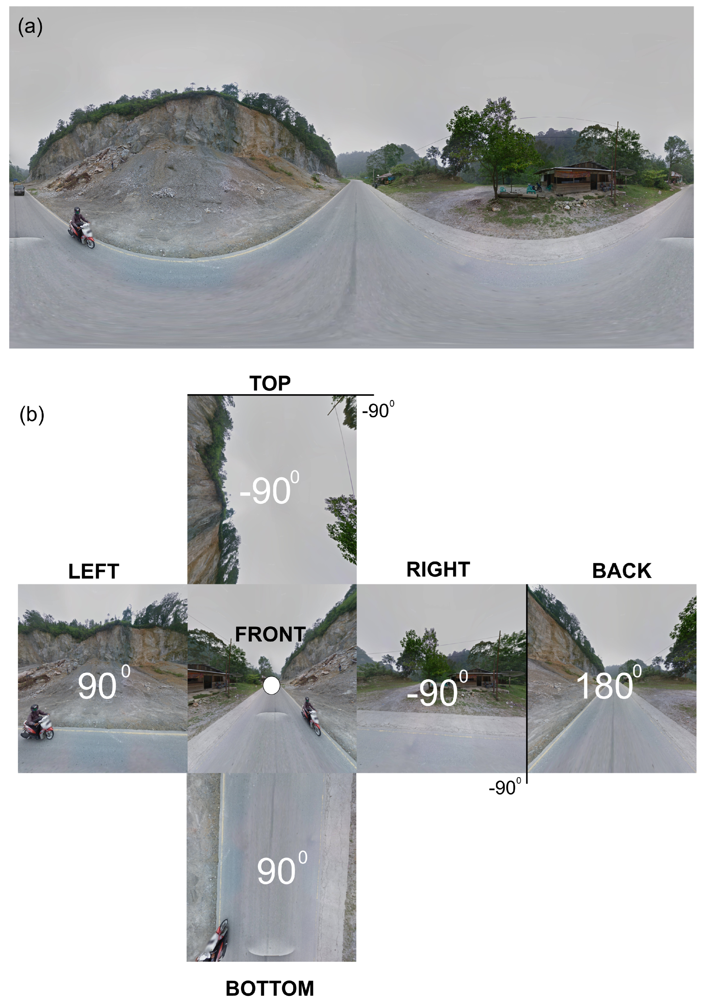
Figure 4.
The image which represent graph of equirectangular and perspective projection image (modified from [35]: (a) Equirectangular image (b) Perspective image.
Figure 4.
The image which represent graph of equirectangular and perspective projection image (modified from [35]: (a) Equirectangular image (b) Perspective image.
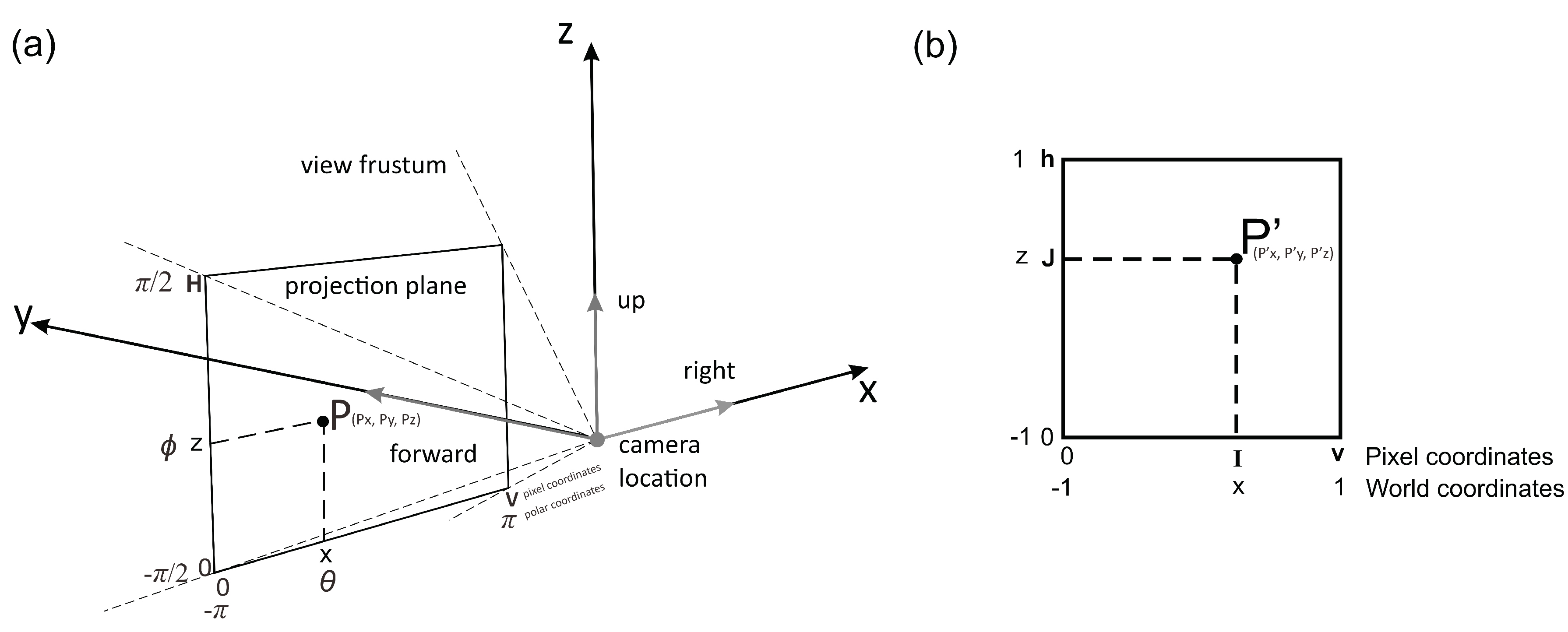
Figure 5.
(a) general view of the rock cliff. (b) Field measurement and identification six set of joint structure on the field (as shown by the yellow and red square (c)). (d) potential failure of wedge and direct toppling from kinematic analysis. (e) detection of joint using coltop3d for point cloud analysis (UAV scanned in 2021).
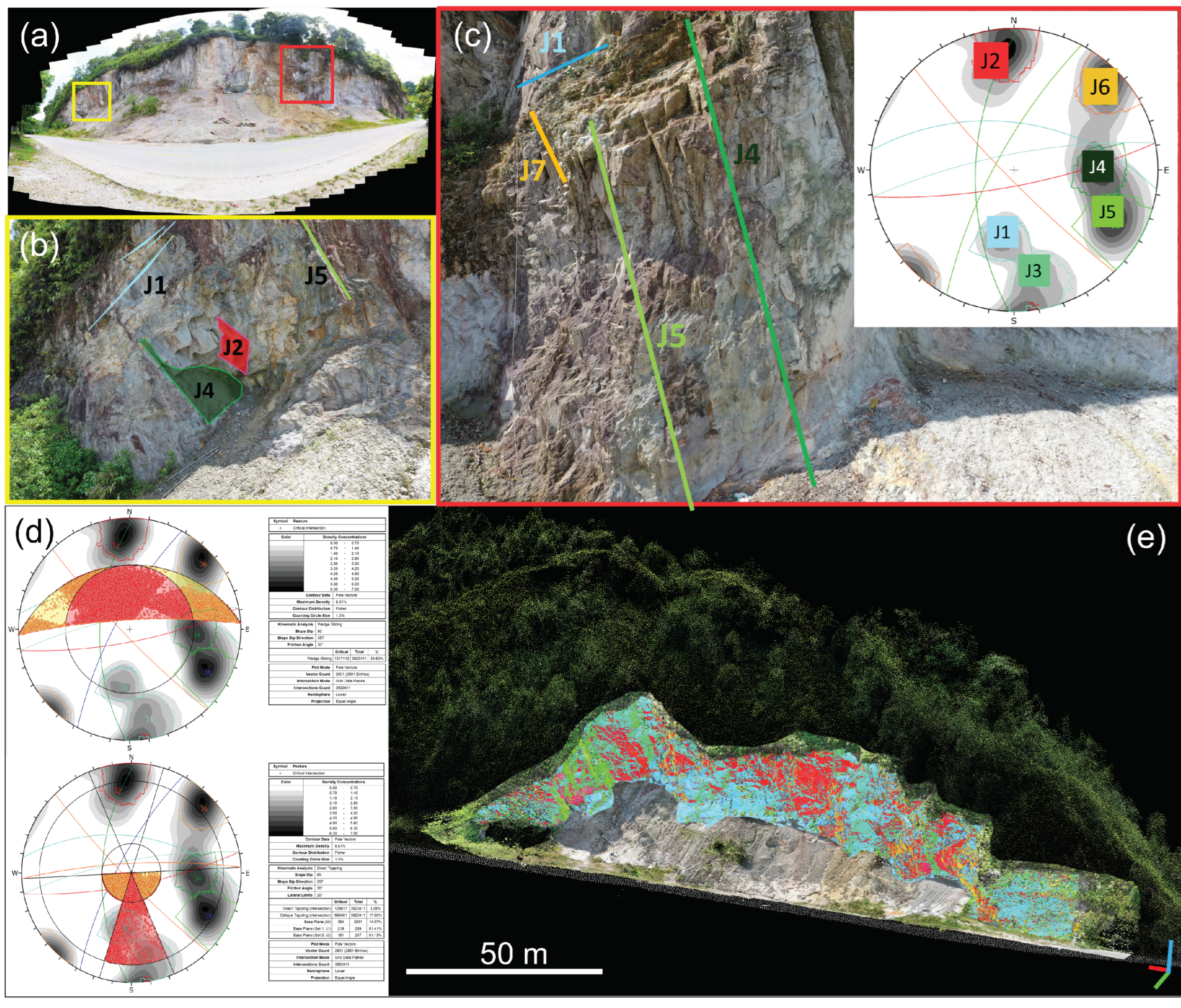
Figure 7.
Cumulative change of rock cliff volume. Blue indicates negative volume change due to erosion or rockfalls; red indicates positive volume change due to deposition.
Figure 7.
Cumulative change of rock cliff volume. Blue indicates negative volume change due to erosion or rockfalls; red indicates positive volume change due to deposition.
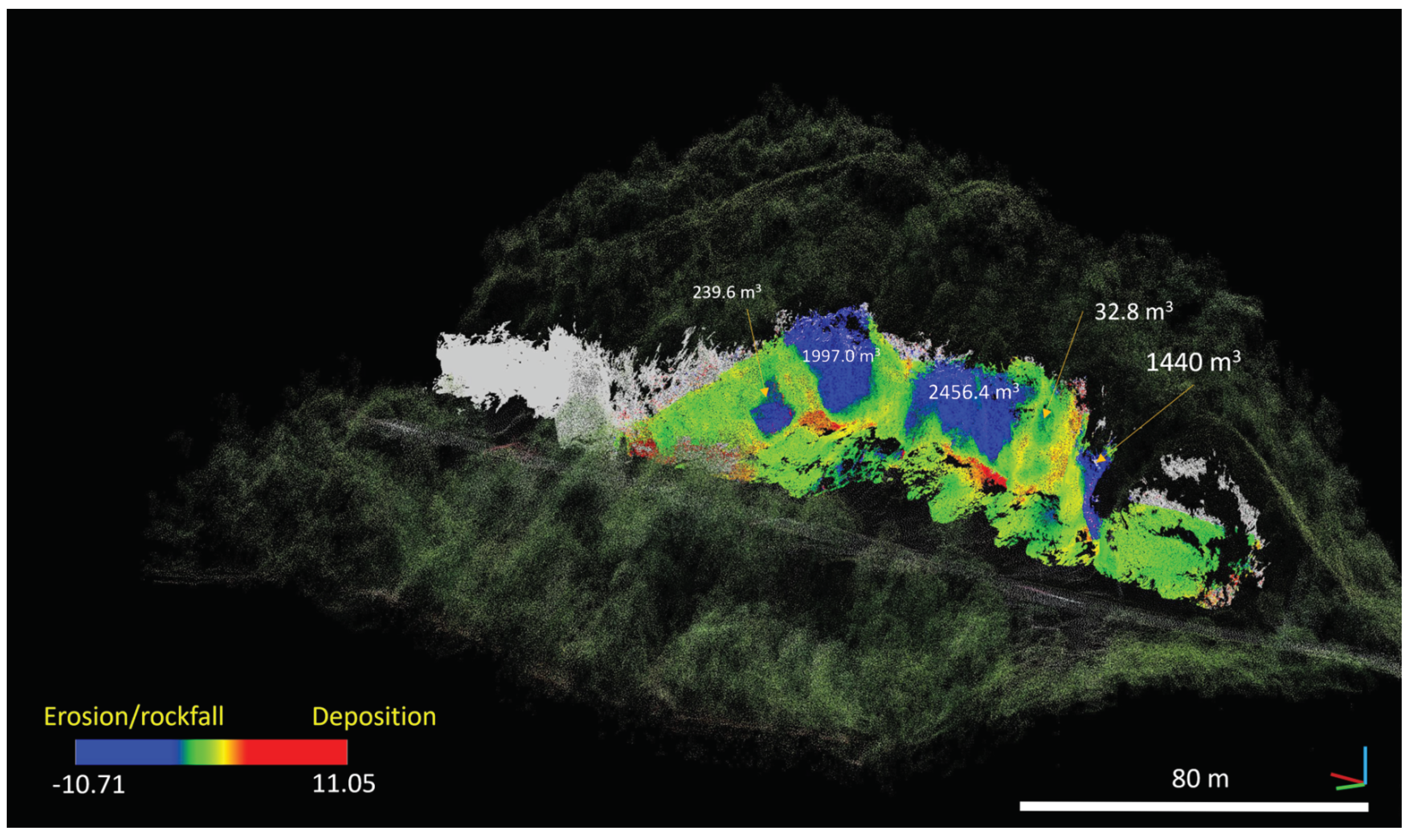
Figure 8.
Magnitude vs frequency of rockfall in Kotopanjang from 2015 – 2021.
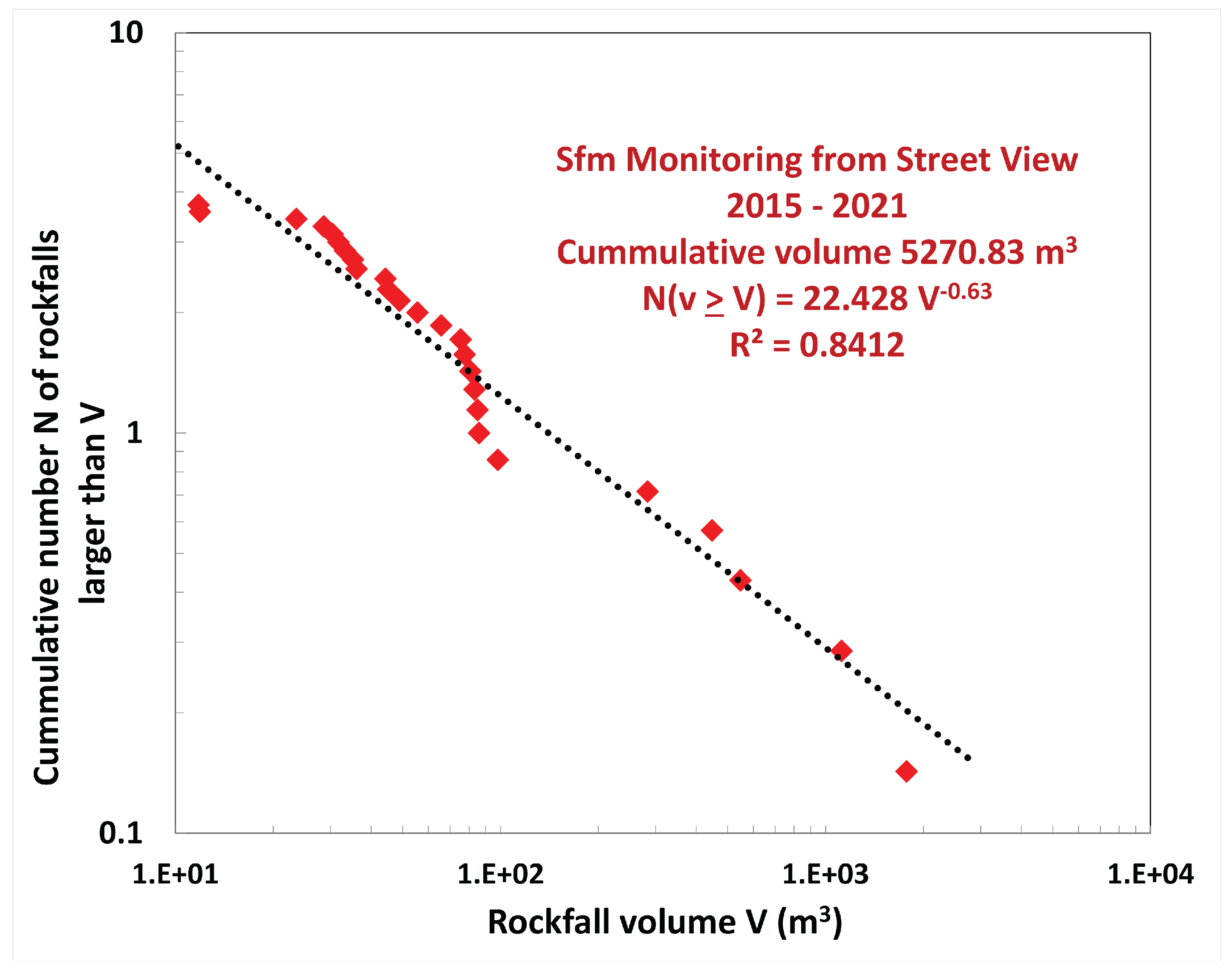
Figure 9.
(a) Spatial variability of intense rainfall every half hour event before rockfall on 13/10/2016 over Kampar area as measured by IMERG ( study show location in the red dot) and (b) Daily precipitations retrieved from IMERG data (2015-2017) and local weather station (BMKG) (2018-2022) with API calculations with regard to the acquisitions of images and event of rockfall.
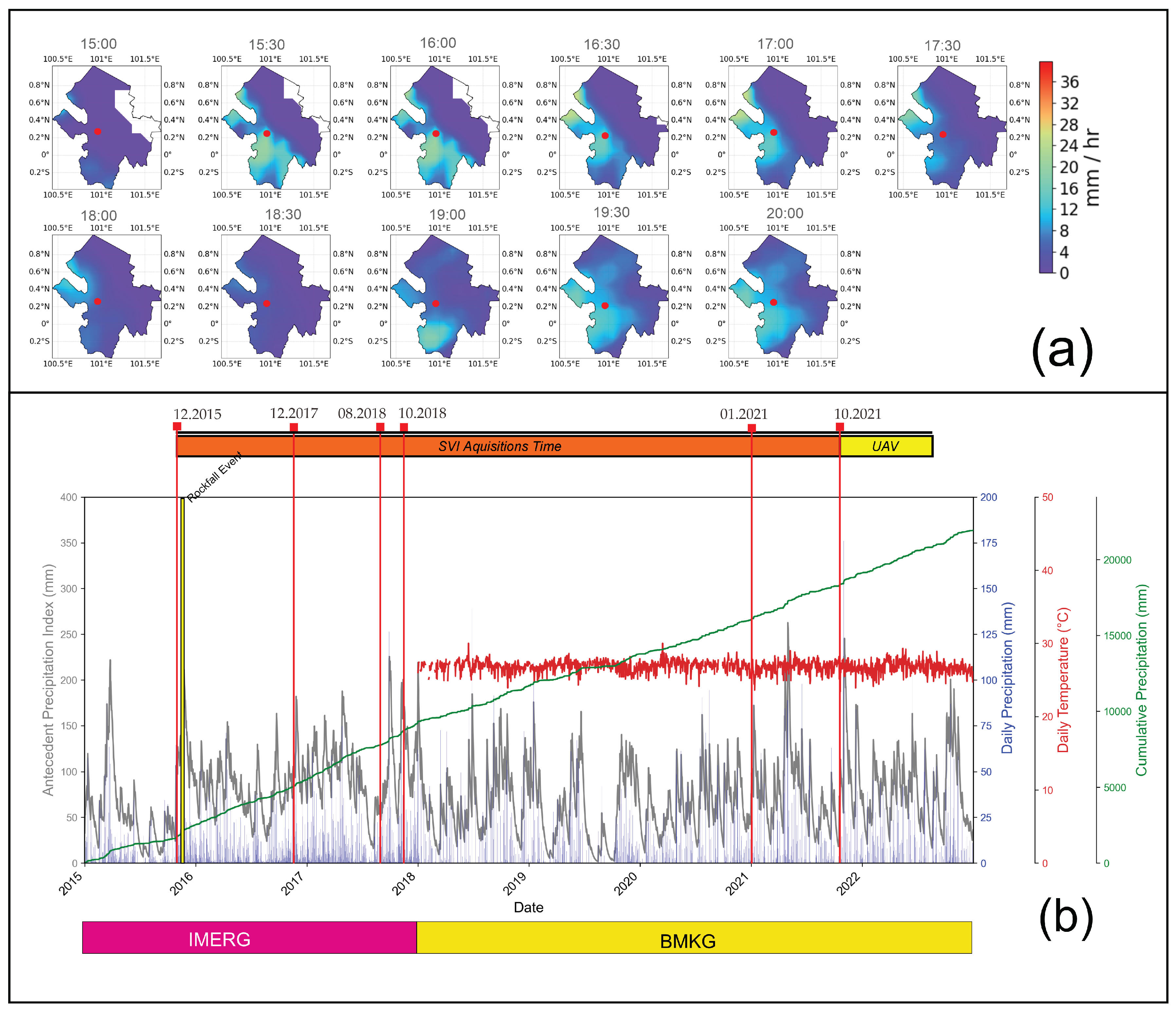
Figure 10.
Image (a) depicts the simulation results based on the 1542 identified source points. (b) presents a comparison of sediment positions at scree slopes with angles less than 20° and greater than 20°. Reach probability and are Maximum velocity presented in (c) and (d), respectively.
Figure 10.
Image (a) depicts the simulation results based on the 1542 identified source points. (b) presents a comparison of sediment positions at scree slopes with angles less than 20° and greater than 20°. Reach probability and are Maximum velocity presented in (c) and (d), respectively.
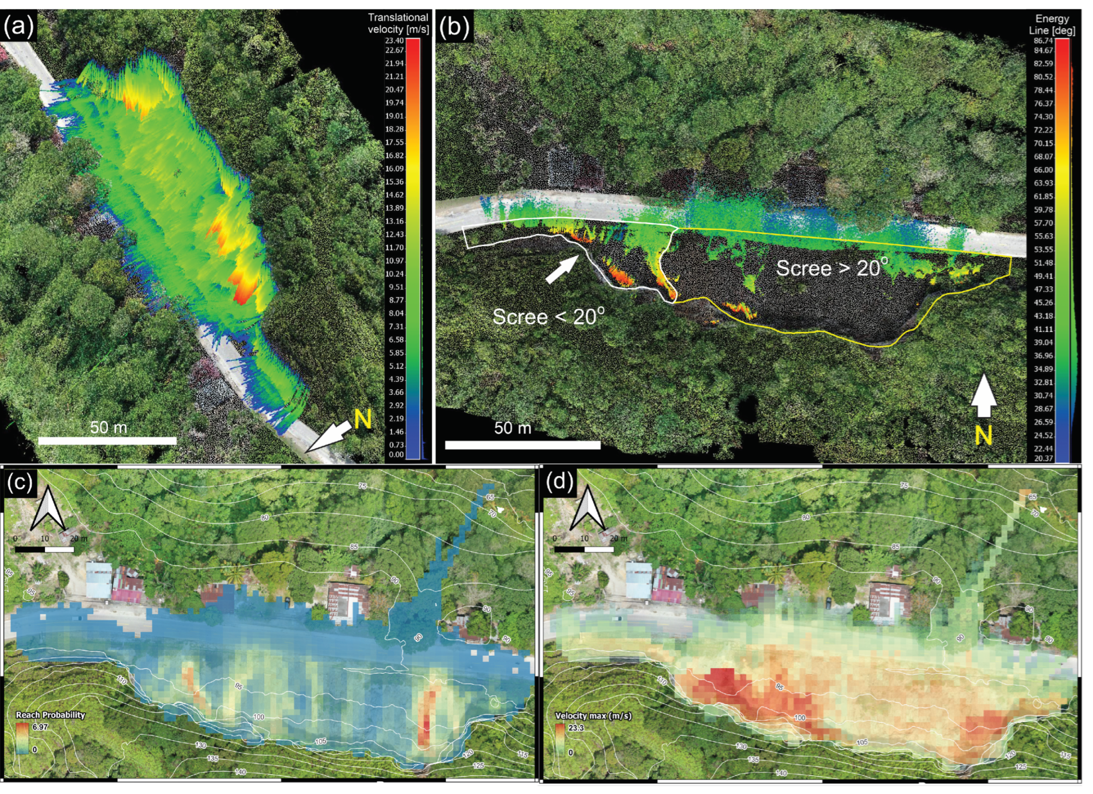

Table 1.
List of Image retrieve from street view imagery and acquisition of UAV.
| Time of Acquisition (MM.YYYY) | No. of Images | Acquisition Method |
|---|---|---|
| 12.2015 | 26 | SVI |
| 12.2017 | 19 | SVI |
| 08.2018 | 26 | SVI |
| 10.2018 | 28 | SVI |
| 01.2021 | 36 | SVI |
| 10.2021 | 280 | UAV |
Table 2.
Cube face and rotation view from initial camera images.
| Cube face | Rotation |
|---|---|
| front | - |
| left | Pan by 90 degrees |
| right | Pan by -90 degrees |
| back | Pan by 180 degrees |
| top | Tilt by -90 degrees |
| bottom | Tilt by 90 degrees |
Table 3.
Dip direction and dip of planar discontinuities measured in the field and from point clouds (using Coltop3D).
Table 3.
Dip direction and dip of planar discontinuities measured in the field and from point clouds (using Coltop3D).
| Discontinuity Set | Dip Direction / Dip from Field Measurements | Discontinuity / m | Dip Direction / Dip from Point Cloud Measurements | Tolerance angle |
|---|---|---|---|---|
| J1 | 5 | ± 15.0 | ||
| J2 | 5 | ± 15.0 | ||
| J3 | 5 | ± 15.0 | ||
| J4 | 5 | ± 15.0 | ||
| J5 | 5 | ± 15.0 | ||
| J6 | 5 | ± 15.0 |
Table 4.
Parameter used for trajectography simulation.
| Parameter | Value |
|---|---|
| 3D terrain model | points |
| Friction Angle | 28o |
| Cohesion | 30 kPa |
| Volume | 1 |
| Density | 2700 kg/ |
| No. of Simulations | 100 each sources |
Disclaimer/Publisher’s Note: The statements, opinions and data contained in all publications are solely those of the individual author(s) and contributor(s) and not of MDPI and/or the editor(s). MDPI and/or the editor(s) disclaim responsibility for any injury to people or property resulting from any ideas, methods, instructions or products referred to in the content. |
© 2025 by the authors. Licensee MDPI, Basel, Switzerland. This article is an open access article distributed under the terms and conditions of the Creative Commons Attribution (CC BY) license (http://creativecommons.org/licenses/by/4.0/).
Copyright: This open access article is published under a Creative Commons CC BY 4.0 license, which permit the free download, distribution, and reuse, provided that the author and preprint are cited in any reuse.


