
Submitted:
12 February 2025
Posted:
13 February 2025
You are already at the latest version
Abstract
Aiming at the strong spatio-temporal coupling relationship between data in the actual industrial production process, which leads to the problem of insufficient reliability and poor timeliness of traditional process anomaly monitoring methods, a time series anomaly monitoring model based on the graph similarity network with multi-scale features is proposed, which can react to the anomalies in the process in a timely and effective manner to guarantee the production safety.First, a graph-building method for spatio-temporally coupled time-series data using multidimensional time-varying feature map embedding is designed to capture the data’s dependence on time, while the topology of the graph is utilized to learn the spatial coupling of the data; second, a graph similarity-based anomaly monitoring strategy is innovatively proposed to measure the anomalies of the process using the difference degree index between the standard normal process data and the monitoring data. Finally, the proposed method is validated using the standard normal operating condition data of the Tennessee-Eastman (TE) process as well as the standard fault data. The experimental results show that the proposed model can identify anomalies more quickly and accurately than other typical methods, which significantly improves the reliability and timeliness of industrial process anomaly monitoring.
Keywords:
Industrial process anomaly monitoring
; Multidimensional spatio-temporally coupled time series data
; Graph similarity computation
; Discrepancy indicators
; Deep learning
1. Introduction
With the continuous expansion of the production scale of industrial processes, the abnormal monitoring of industrial process operation status is of great significance in improving product quality and ensuring production safety[1,2]. Distributed control system (DCS) in the field of industrial control is widely used, so that the complex industrial process of multi-dimensional spatial and temporal coupling of real-time acquisition and processing of time series data has become a reality. The in-depth analysis of process data can accurately reflect the operating status of industrial processes, providing unprecedented opportunities for process anomaly monitoring and diagnosis.
Data-based process monitoring methods have become one of the hot directions in the research field of industrial operation conditions, but the existing anomaly monitoring methods face many challenges[3,4,5,6]. First, multivariate statistics-based process anomaly monitoring methods usually monitor whether the statistics exceed the control limits to determine whether the process is anomalous or not. For example, Principal Component Analysis (PCA) detects anomalies by reducing dimensionality and reconstruction errors and is suitable for high-dimensional linear data[7,8]; Independent Component Analysis (ICA) detects anomalies by separating independent components, which is suitable for complex, non-Gaussian signals[9]; Partial Least Squares (PLS) detects process anomalies and assists in troubleshooting by extracting latent variables and monitoring residuals or statistics[10]. Although the above methods show certain advantages when dealing with high-dimensional linear or non-Gaussian data, they are difficult to effectively capture the complex nonlinear relationships in spatio-temporal data when dealing with multi-dimensional spatio-temporal coupled time series data, and at the same time, they ignore the time-dependence in the data, which leads to insufficient anomaly detection ability in the temporal dimension, and limits the effectiveness of their practical application in complex industrial processes. Second, deep learning based process anomaly monitoring methods such as convolutional neural networks predict target values by modeling the process through a black box model, and anomaly monitoring is performed by comparing the predicted values with the observed values. While CNNs are able to capture local patterns and spatial dependencies, their inherent local feel-good field design makes it difficult to model global spatio-temporal dependencies, especially in industrial processes where there are long-range dependencies between variables, and CNNs are often limited in their performance[11,12]. Long and short-term memory networks are suitable for time-series data and are able to capture temporal dependencies, although their weak modeling ability for spatial features and significant increase in computational complexity and training time when dealing with high-dimensional multivariate data limit their application in real industrial scenarios[13,14]. In the face of industrial process anomaly monitoring with multidimensional spatio-temporal coupled time series data, deep learning-based methods face a series of deep challenges and limitations in both theoretical and practical applications.
Industrial processes have their unique operational characteristics: first, production processes often need to be maintained in steady state or show periodic changes for a long time to ensure the stability of product quality; second, due to the high reliability of modern industrial systems, the probability of failures occurring is extremely low, leading to a scarcity of anomaly samples, which brings significant difficulties to data-driven anomaly detection methods. However, this specificity also provides new research ideas for anomaly monitoring. The properties of steady-state processes imply that when an abnormality occurs, there is a significant difference between the abnormal working condition and the standard normal working condition. Therefore, accurate identification of abnormal states in a production process can be achieved by effectively capturing this dissimilarity through mathematical methods[15,16]. Further, the measure of dissimilarity between working conditions can be transformed into a similarity calculation problem, which provides a quantifiable evaluation framework for anomaly detection. Traditional similarity calculation methods, such as Euclidean distance calculating similarity by interval distance, are applicable to the scenario of data distribution uniformity and low dimensionality, facing high dimensional data is vulnerable to the influence of “dimensional disaster”, resulting in the loss of differentiation of distance calculation[17,18]; cosine similarity measures the similarity by calculating the angle between the vectors, which is applicable to the scenario of text data or high-dimensional sparse data. The cosine similarity measures the similarity by calculating the angle between vectors, which is suitable for textual data or high-dimensional sparse data, but when facing spatio-temporal heterogeneity of industrial data, it only pays attention to the direction of the vectors and ignores the magnitude of the vectors, so its ability of characterization is limited[19,20]; Dynamic Time Warping (DTW) is able to deal with the problem of nonlinear alignment of the time series in the time axis, and thus it has a certain advantage in the analysis of time series. However, DTW has higher computational complexity and ignores the spatial coupling relationship between the data, so its performance is limited when dealing with industrial data with strong spatio-temporal coupling characteristics[21,22]. How to design more adaptable similarity measures by combining the specificity of industrial processes is still an important direction of current research.
The graph-based similarity computation method opens up a brand new research direction for similarity computation and demonstrates a wide range of application value in several academic fields. In social network analysis, by comparing the structural features of users’ social graphs, the similarity of users’ behavioral patterns can be revealed, thus assisting in community detection and group delineation; in the field of bioinformatics, graph similarity algorithms have been used to analyze protein interaction networks and gene regulatory networks, and thus infer protein functions or identify evolutionary homology; in the field of computer vision, graph structure-based image matching techniques rely on graph similarity computation; in natural language processing, text graph similarity provides a new research perspective for semantic analysis and text matching. These applications fully reflect the importance of graph similarity computation in interdisciplinary research. Therefore, it is of significant research value to utilize the advantages of graph theory to understand the multidimensional spatio-temporal coupled time series data of industrial processes, and thus to adapt to the specificity of industrial processes. Bai et al. proposed a new neural network-based method designed to reduce the computational burden while maintaining good performance. The method first designs a learnable embedding function that maps each graph to an embedding vector, thus providing a global summary of the graph. The method also designs a pairwise node comparison strategy to complement the graph-level embedding with fine-grained node-level information, and finally combines two sets of features for graph similarity computation[23].
Based on the above analysis, this paper addresses the difficulties faced by multidimensional spatio-temporally coupled time series data of industrial processes in anomaly monitoring, and innovatively proposes to apply graph similarity to the field of non-stationary industrial process anomaly monitoring on the basis of graph similarity calculation method. In this paper, we design a graph similarity-based industrial process anomaly monitoring model and application, aiming at extracting features on the time series, while capturing the spatio-temporal dependence and the complex coupling relationship between variables, to realize the effective monitoring of industrial process anomalies. The model constructs the spatio-temporal graph structure of the data through the graph embedding strategy of multidimensional time-varying features, maps the multivariate time series data in the two-dimensional space to the graph space while considering the temporal dependence of the data, and aggregates the features by using graph convolution network (GCN) in order to capture the complex coupling relationship between the variables, so as to realize the comprehensive modeling of the spatio-temporal dependence. Further, this paper introduces the method of graph similarity computation, based on the traditional method of feature integration only in the two perspectives of global features of topology and local differences of nodes, and adds the difference features of the adjacency matrix to participate in the similarity analysis, which effectively solves the shortcomings of the traditional similarity computation method in the modeling of high-dimensional coupled data, noise interference, and nonlinear relationships among variables. Through this multi-level similarity analysis, the model is able to more accurately identify and monitor abnormal behaviors in industrial processes. Experimental results show that the model proposed in this paper is not only able to accurately monitor process anomalies, but also has strong robustness and generalizability, which can adapt to the needs of industrial scenarios with few samples of anomalous data and high real-time requirements. The model outperforms existing benchmark methods on multiple industrial datasets, especially when dealing with high-dimensional, nonlinear coupled data. In addition, the computational efficiency of the model is high enough to meet the demands of real-time monitoring of industrial processes. This study provides a new framework and method for industrial process anomaly monitoring, which has important theoretical significance and practical application value. From the theoretical point of view, the anomaly monitoring model based on graph similarity provides a new idea for the analysis of multidimensional spatio-temporal coupled time series data, and extends the application scope of graph neural networks in industrial process monitoring. From the practical application point of view, the model can effectively improve the reliability and timeliness of industrial process anomaly monitoring, which provides a strong guarantee for the stability and safety of industrial production.
2. Materials and Methods
In this section, the relevant methods involved are introduced to facilitate a better understanding of the model architecture proposed in this paper.
2.1. Granger Causality
Granger causality is a statistical method for testing causal relationships in time series data, proposed by economist Clive Granger. The core idea is that X can be considered to have Granger causality for Y if information about a time series X in the past significantly improves the predictive power of another time series Y. Specifically, tests of Granger causality are usually based on the F-test or chi-square test, which determines the significance of causality by comparing the goodness-of-fit (e.g., the residual sum-of-squares or log-likelihood values) of models that include and do not include the potential causal variables. The method is widely used in time series analysis to reveal dynamic dependencies among variables and provides a tractable framework for causal inference[24,25,26].
Suppose there are two time series and , where t denotes time. For a regression model containing past values of and is expressed as follows:
Where is the lag order of , is the regression coefficient, and is the error term, respectively. The F-statistic is calculated using the following formula:
Where T is the sample size, is the lag order of , and is the square of its residuals for the model without causality and the model with causality, respectively. If the F statistic is greater than the critical value, the original hypothesis is rejected and are considered to have Granger causality.
2.2. Autoencoder
Autoencoder is a neural network-based nonlinear dimensionality reduction technique widely used in data compression and feature extraction tasks. Its core idea is to map the original high-dimensional data to a low-dimensional potential space through the collaborative work of encoder and decoder, and reconstruct the original data in that space. This process can effectively capture the nonlinear structure in the data, thus significantly reducing the data dimensionality while retaining the main feature information, and providing support for subsequent data analysis and modeling[27,28,29].
The basic steps of an autoencoder include data preprocessing, model training, and potential space extraction. First of all, the input data usually needs to be normalized to eliminate the effect of the magnitude difference on the model training. The normalization formula is as follows:
Where is the time series data of sensor i, is the mean value of the time series data of sensor i, and is the standard deviation of the time series data of sensor i. The data matrix is obtained after the normalization is completed.
The training process of the autoencoder optimizes the model parameters by minimizing the reconstruction error. The reconstruction error is usually calculated using the mean square error (MSE) as the loss function, which is given in the following formula:
Where is the original data, is the reconstructed data, and n is the number of samples.
During the training process, the encoder maps the input data to a low-dimensional potential space H, whose dimension is much lower than that of the original data. The potential space H is represented as follows:
Where f is the nonlinear transform function of the encoder and is the weight parameter of the encoder. The decoder then reconstructs the original data from the potential space H and its output is:
Where g is the nonlinear transformation function of the decoder and is the weight parameter of the decoder.
Through training, the autoencoder is able to learn a low-dimensional representation of the data H, which captures the main feature information of the data. Different from the traditional data dimensionality reduction methods, autoencoders are able to handle nonlinear data structures, and thus usually perform better on complex data sets. In addition, the potential spatial dimensionality of the autoencoder can be flexibly adjusted according to practical needs, thus providing greater flexibility for data compression and feature extraction.
2.3. Graph Convolutional Network
Graph convolutional network (GCN) proposed by Kipf et al. significantly improves the efficiency and maneuverability of the model by simplifying the spectral graph convolution operation. The core idea lies in iteratively updating the node representations using the aggregation mechanism of local neighborhoods to effectively capture the topological information in the graph structure.Specifically, GCN avoids complex frequency-domain transformations by approximating the spectral graph convolution as a linear combination of first-order neighborhoods, enabling the model to be operated directly in the null domain and reducing the computational complexity. This design not only preserves the global properties of the graph structure, but also enhances the expressive power of the model by realizing the gradual integration of higher-order neighborhood information through multi-layer stacking[30,31,32,33].Define the graph structure as , where V denotes a node in the graph and , and E denotes an edge.The nodes are usually represented by the matrix , n denotes the number of nodes,and m denotes the dimension of the features. Define its adjacency matrix to be a square matrix of order n, where the value of denotes whether there is an edge connection between vertex i and vertex j. Define the matrix and the degree matrix as follows:
Where , is a unit matrix of size with diagonal element 1. Each layer of convolution operation of GCN can be represented as:
Where is the ReLU activation function. When , is the input feature matrix, usually denoted as X, where each column corresponds to the feature vector of a node. is the trainable parameter matrix for linear transformation of the features. is the normalized representation of the adjacency matrix , making the aggregation operation more stable. is the graph node feature representation matrix at layer l. is the updated graph node feature representation matrix.
3. Anomaly Monitoring Model for Industrial Processes Based on Graph Similarity
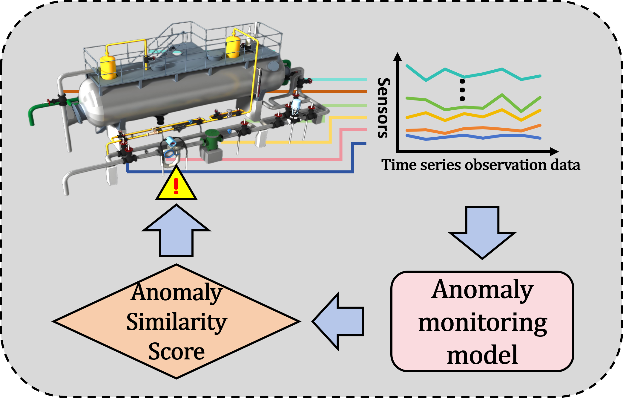
The time series anomaly monitoring model of graph similarity network based on multi-scale features consists of two parts: time series data processing module and graph similarity calculation module, and the model structure is shown in Figure 1. The time series data processing module takes two sets of time series data from standard normal working conditions and monitoring process as input, and completes the transformation from two-dimensional time series data to graph time series set through the multidimensional time-varying feature graph embedding process; the graph similarity computation module takes the above two sets of graph time series sets as input, and obtains the similarity scores of the two graph structures in the same moment after a series of feature extraction and aggregation processes, and then converts them into graph differences to complete the process anomaly monitoring and alarm.
The multidimensional time-varying features proposed in this paper are defined as the historical data based on the moment t. The length of the time window is taken as m. The combination of the original time features of the data at the moment and the statistical features of the time series data computed based on the original time features are extracted as the feature representation of the data values of t at the current moment, and the multidimensional time-varying feature embedding is repeated for t as t progresses step by step in the time series, until t is the current moment. The graph structure usually consists of nodes, edges, edge weights, node features and other elements. When mapping industrial process data into the graph space, each industrial sensor can be represented as a node in the graph structure, and the coupling relationship or physical connection between sensors can be treated as an edge connected to the node.
Complex industrial processes with dynamic and non-stationary features generate multi-dimensional spatio-temporal coupled time series data with high time dependence, based on which, this paper proposes a time series data processing module to deeply extract the time dependence of the data, and at the same time, utilize the graph structure to capture the spatial coupling relationship among sensors, and then monitor the process anomalies timely and accurately through graph similarity computation. Specifically, firstly, in the time series data processing module, Granger causality calculation is used to determine the dynamic dependency relationship among sensors, while data downscaling technology is used to construct a low-dimensional space, and furthermore, a multidimensional time-varying feature map embedding strategy is adopted to expand the time series data in the two-dimensional space to the three-dimensional space and eventually mapped to the graph space, completing the graph structure of the multidimensional spatio-temporally coupled time series data. The graph structure provides a more intuitive expression for the visualization of data relationships, and at the same time, the graph space data can effectively capture the nonlinear coupling relationship between variables, thus enhancing the generalization ability and prediction accuracy of the model. Second, in the graph similarity computation module, node features of the graph structure are extracted using graph convolutional network aggregation to make them globally relevant. Further, global features at the graph level and local features at the node level are captured respectively using Neural Tensor Networks and histogram statistics, and are inputted to the fully connected layer for similarity score output through feature aggregation. Through the multi-level feature capture and feature aggregation and fusion mechanism, the global structure and local details of the graph can be considered comprehensively, which significantly improves the accuracy and robustness of graph similarity calculation. In the absence of a large number of data anomaly markers, the model realizes unsupervised monitoring of industrial process anomalies by outputting the deviation score of the current production process from the standard normal production conditions as the basis for judging the anomalies. The model shows significant advantages in dealing with complex industrial process multidimensional spatio-temporal coupling time series data anomaly monitoring, which can effectively deal with complex industrial data, improve the accuracy and robustness of anomaly detection, and at the same time has a strong generalization ability, which is applicable to a variety of industrial scenarios. Through the combination of global and local features, the module can reflect the operating status of the system more comprehensively and provide reliable support for anomaly monitoring.
3.1. Time Series Data Processing
When dealing with multidimensional spatio-temporally coupled time series data of industrial processes, data dimensionality reduction and compression is a key step to improve the computational efficiency due to data redundancy and complexity. In this paper, the initially collected industrial sensor time series data is firstly represented as a set . In order to reveal the potential dynamic connections between sensors, Granger causality analysis was first used to explore the causal dependencies between the sensors. Next, an autoencoder is used to downscale the data. By minimizing the error between the input data and the reconstructed data, the self-encoder is able to learn an efficient low-dimensional representation of the data while capturing the nonlinear relationships in the data, thus retaining the key information in complex industrial data more effectively. By analyzing the distribution of potential spatial features and their contribution to the reconstruction error, sensor data that play a key role in the dimensionality reduction process can be identified, providing a more robust feature representation for subsequent anomaly detection.
The time-series causality analysis reveals the dynamic dependencies between sensor data, while the autocoder helps to identify the variables that have a major influence by quantifying the contribution of each sensor data. Combining these methods can reduce the dimensionality of the data while retaining key information, thus improving the efficiency and accuracy of the subsequent analysis. The specific calculation formula is shown below:
By processing the industrial process sensor data, the first k main variables calculated by the autoencoder are calculated and the sorted first k sensor data are selected for normalization based on the contribution of the respective variables as the time series data set of the industrial process, where , is the time series data of the sensor i.
For the t-moment data of , the time window length is taken, and the original temporal features and statistical features of the time series data at the moment of are used as the feature representation of the moment t. Multi-temporal dynamic feature embedding is repeated for t as t progresses step by step in the time series, so that the original time series data is extended to the three-dimensional space. The moment t data of embedded with dynamic multitemporal features can be expressed as:
Multidimensional time-varying features are an effective structure for time domain oriented data processing, which can accurately capture the dependency and dynamic fluctuation of data on time series. The multidimensional time-varying feature graph embedding process proposed in this paper is shown in Figure 2.
The core of multidimensional time-varying feature graph embedding lies in mapping two-dimensional spatio-temporal data into the graph structure space, and constructing graph structures reflecting the system state at the current moment for the data in each time window. These time-ordered graph slices are concatenated through the time dimension to form a dynamic graph sequence, thus completely characterizing the spatial coupling properties and temporal evolution laws of sensor networks in industrial processes. This graph structure-based modeling approach has significant advantages: in the spatial dimension, the graph structure can effectively capture the complex correlations among sensors; in the temporal dimension, the dynamic graph sequence can accurately describe the state evolution of the system. By combining the theories and methods of graph theory and graph neural networks to characterize the macroscopic behavioral patterns and microscopic fluctuation characteristics of industrial data, it provides a powerful tool for the analysis and modeling of complex industrial systems.
3.2. Graph Similarity Calculation
In this section, the graph similarity calculation is described in detail.The multidimensional spatial and temporal coupling of the industrial process of the standard normal operating conditions of the graph time series set and online monitoring data after time series data processing from the two-dimensional space mapped to the graph space, the formation of graph time series set ,,where , denotes the graph structural data at the moment , including the nodes, node multidimensional time-varying features, edges, and other graph attributes. is used as the module input, and the graph convolutional network is used to reaggregate all node features based on neighboring nodes to obtain a new node multidimensional time-varying feature representation with global attributes, which is calculated as follows:
Where , is the set of first-order neighbors of node n plus n itself, is the degree of node n plus 1, is the weight matrix associated with the l-th GCN layer, is the bias term, and is an activation function such as .
Overall, the graph convolution operation aggregates features from the first-order neighbors of a node, and when multiple graph convolution operations are performed, each node then has a feature representation of the global attributes. The graph similarity computation process after aggregation by GCN features is schematically shown in Figure 3.
3.2.1. Graph Level Feature Aggregation
The graph level feature aggregation can encode the structure and feature information of the graph, and through the aggregation of two graph level features, it can provide an important basis for judging the similarity between two graphs. In the initial stage of graph similarity computation module of Figure 1, different colors denote different node features and after GCN the node features are re-aggregated and the colors are changed accordingly. After the graph structure has gone through multiple layers of GCN (3 layers are taken in this paper), the node embeddings are ready to be fed into the Global Attention Awareness module (O-Att). In order to characterize each graph structure using a set of features, a weighted aggregation of the nodes’ features can be used. Therefore, in order to determine which nodes are more important and should receive more weights, we propose the Global Attention Awareness Module that allows the model to learn weights guided by a specific similarity metric.
The input node multidimensional time-varying features are represented as , where the nth row is the multidimensional time-varying feature representation of node n . First compute the simple global average vector of the node features in the graph , and then perform a nonlinear transformation as follows:
Where is a learnable weight matrix. The global average vector C adaptively computes an attention weight for each node for the similarity measure of the global structural features of the graph by learning the weight matrix. For node n, take the inner product between the global average vector c and its node features, and the inner product result is used to decide that nodes that are similar to the global average vector should receive higher attention weights. Finally the sigmoid function is applied to the above computed results to ensure that the attention weights are within the range (0, 1). Finally, the graph level feature aggregation result H is the weighted sum of all node features. The above attention mechanism can be expressed as follows:
Where is the sigmoid function .
The weighted graph-level feature aggregation result is thus obtained for modeling the relationship between two graph-level embeddings using a neural tensor network (NTN):
Where is the weight tensor, denotes the tandem operation, is a weight vector, is a bias vector, is an activation function, K is a hyperparameter, and the control model is the number of interaction (similarity) scores generated for each graph embedding pair.
3.2.2. Comparison of Node-Level Features
Node-level information (e.g., node feature distributions and graph sizes) may be lost as a result of computing graph-level feature aggregation. In graph sequence data of industrial processes, the key to the difference between two graphs lies in the difference in node features, which is often difficult to reflect by graph level features. Therefore node-level feature comparison is also a key part of the process of computing graph similarity.
The pairwise interaction score between nodes is calculated by the following equation:
Where , is the characteristic representation of node i and node j. Since the node-level features are not normalized, a Sigmoid function is applied to ensure that the similarity score is in the range (0, 1). In order to ensure that the model’s representation of the graph structure is invariant, a more efficient and natural way of utilizing S needs to be considered. Therefore, it is taken to extract its histogram feature: , where B is the hyperparameter (in this paper ) that controls the bins in the histogram. The histogram feature vector, denoted as , is normalized and output as a key part of the graph similarity computation.
3.2.3. Difference Computation after Adjacency Matrix Spreading
After obtaining the graph level features and node differences, we focus our attention on the adjacency matrix in order to capture the more detailed differences between the two graphs. The adjacency matrices of the two graphs are flattened into one-dimensional vectors, where each element denotes the degree (i.e., the number of neighbors) of the corresponding node. Specifically, for graphs and , their adjacency matrices are and , respectively, where ,n are the number of nodes. First calculate the degree vector for each node: Then, the values of the corresponding positions of these two degree vectors are subtracted to obtain a new vector:
Where the length of is the number of nodes n, and each element represents the difference between the degrees of the corresponding nodes in the two graphs.
Through the above calculation, the difference relationship between the neighboring matrices of two graphs is obtained more intuitively, which provides the basis for graph similarity calculation.
3.2.4. Similarity Score Calculation and Exception Alarm
The coarse global information from graph-level feature aggregation is combined with the fine-grained information captured by node-level feature comparisons as well as the difference features of the adjacency matrix in order to provide a comparative, comprehensive graph structure characterization of the model. In the final stage, a standard multi-layer fully connected neural network is applied to gradually reduce the dimensionality of the similarity score vector. Finally, a score ∈ R, is predicted
and compared to the ground truth similarity score using the following mean square error loss function:
Where is the set of training graph pairs and is the true similarity between , obtained by normalizing the Euclidean distance of the node vectors:
Where is the Euclidean distance formula, denotes the coordinate values of node P and node Q in the kth dimension, respectively, and n denotes the number of dimensions of the space.
The calculated similarity score ∈ R, is transformed into the difference score between [0,1],
with larger values indicating larger differences. After many validations, the anomaly exceeding
threshold is usually set to 1.1-1.5 times of the average value of the difference score under normal
operating conditions, and the specific value needs to be set individually according to different operating
conditions. By comparing the deviation of the difference score calculated by the model with the overrun
threshold, the abnormal state at the current moment is determined.
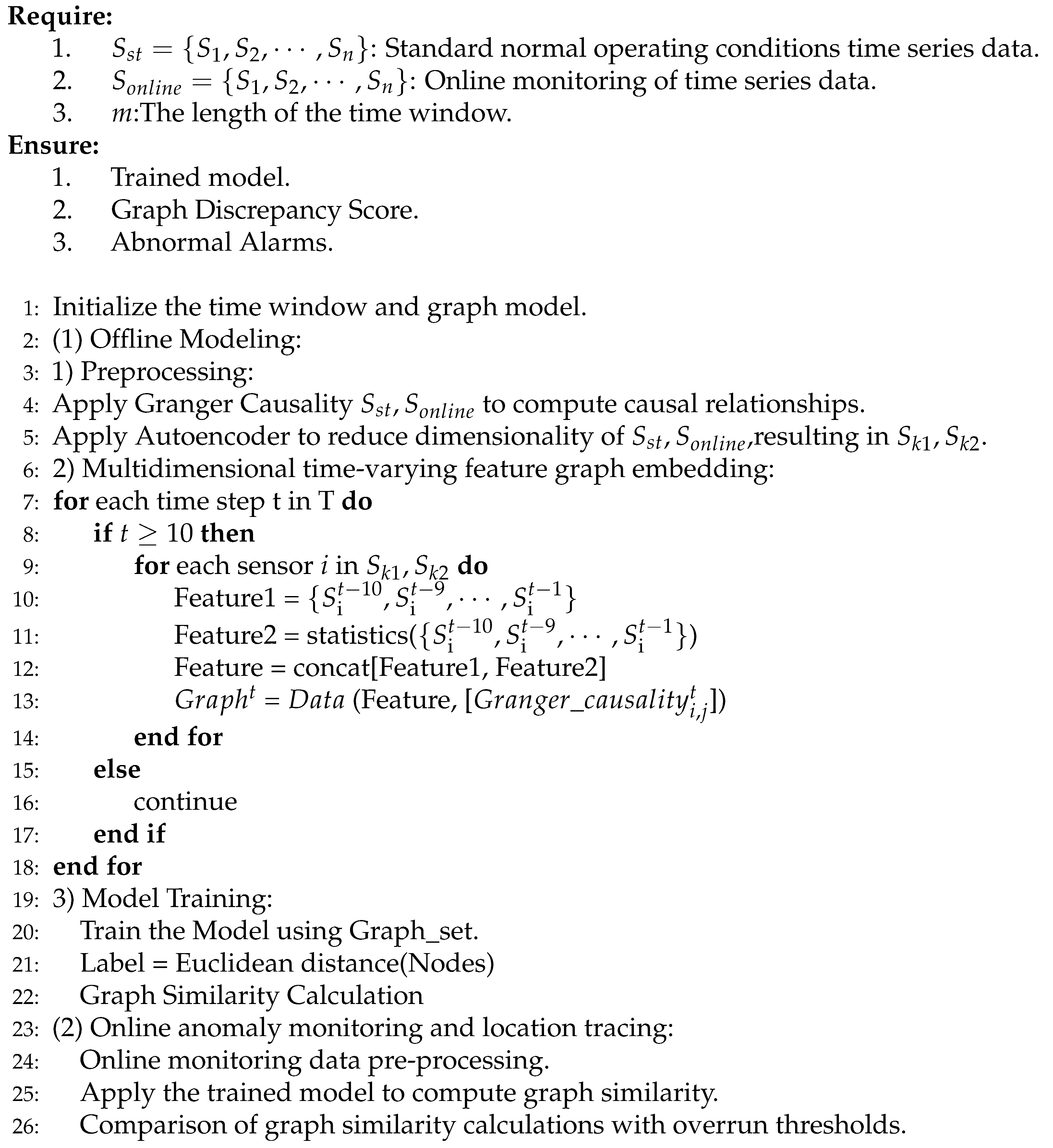
3.3. Application Steps
Note:
- : Data of sensor i at time t.
- : Sensor data after dimensionality reduction.
- Feature1: Raw time characteristics of dynamic data.
- Feature2: Dynamic statistical characteristics of dynamic data.
- Feature: Multidimensional time-varying characteristics of time series data.
- : Graph structure of data at time t.
- Graph_set: A set of graph sequences after time series data is mapped to graph space.
| Algorithm 1 Anomaly monitoring model of industrial processes based on graph similarity and applications |
 |
4. Experimental Applications
This section validates the validity and reliability of the application of the graph similarity network time series anomaly monitoring model based on multi-scale features proposed in this paper based on Tennessee-Eastman (TE) process data. The dataset used and a discussion of the experimental results are presented in the following section.
4.1. Introduction to the Tennessee-Eastman (TE) Process Dataset
Based on the actual chemical reaction process, Eastman Chemical Company has developed an open and challenging chemical modeling simulation platform, the Tennessee Eastman (TE) simulation platform. The data generated by this platform are time-varying, strongly coupled and nonlinear, and are widely used to test control, monitoring and troubleshooting models of complex industrial processes.
Figure 4.
Schematic of the Tennessee-Eastman (TE) process
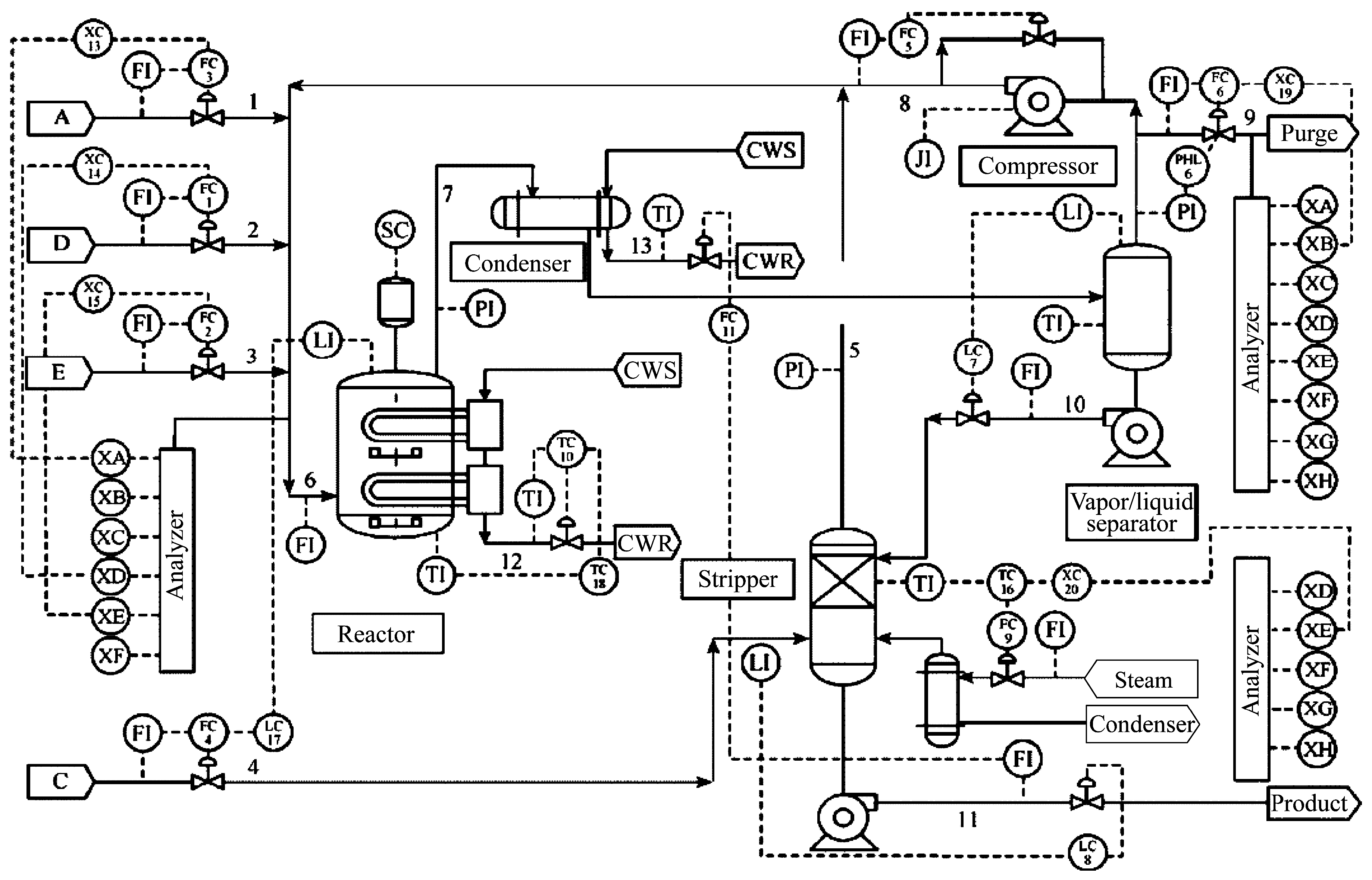
The TE process dataset consists of a training set and a test set, and the training set and test set data consist of data from 22 different simulation runs, respectively, with each sample data containing 12 manipulated variables, 22 continuous process measurement variables, and 19 component measurement variables. The training set samples are numbered as d00.dat to d21.dat, and the test set samples are numbered as d00_te.dat to d21_te.dat. where d00.dat and d00_te.dat are the samples under normal operating conditions. d00.dat training samples are obtained under 25h running simulation. The total number of observations is 500; d00_te.dat test samples were obtained under 48h running simulation and the total number of observations is 960. d01.dat to d21.dat are training set samples with faults and d01_te.dat to d21_te.dat are test set samples with faults. Each sample in the training set∖test set represents a fault. Where the training set samples with faults were obtained under a 25h running simulation. The simulation starts without faults and faults are introduced at the 1h moment of the simulation time, but the observations are collected only after the introduction of the faults, i.e., there are only 480 observations. The test set samples with faults were obtained under a 48h running simulation, the faults were introduced at the 8h time moment and a total of 960 observations were collected, of which the first 160 observations were normal data.
4.2. Experimental Analysis and Discussion of Results
4.2.1. Experimental Modeling
Considering the diversity of normal operating conditions data distribution, the combination of normal operating conditions time series data and some fault conditions time series data in the dataset is used as the training set to model and train the model.
Granger causality was used to determine the causal relationship between the sensors selected by the above process. The maximum lag order of 9 was chosen and the relationship test was selected as residual squared and F-test with p-value less than 0.05 and this was used as the edge of the connection between the nodes. The causality results are shown in Figure 5.
Dimensionality reduction and data compression operations on sensor datasets using autoencoder.The selection of potential dimensions with a cumulative explanatory power of 80% of the autoencoder reconstruction error and the eventual selection of 24 sensor variables as key features that can effectively characterize industrial processes significantly reduces the dimensionality of the data. The selection results are shown in Figure 6 and Table 1.
From the above Granger causality calculation results and with reference to expert experience, a multidimensional time-varying feature graph embedding work is carried out based on the main influencing variables in the downscaling results of the autoencoder data, which extends the two-dimensional time-series data to the three-dimensional space, and then maps it to the graph space, so as to establish a set of graph sliced sequences based on the multi-temporal features, where each layer of the graph structure is schematically shown in Figure 7.
The industrial condition data from TE dataset are individually built into a set of graph slice sequences based on multi-temporal features according to the above steps. The proposed industrial process anomaly monitoring model based on graph similarity computation takes two time series sets of the same length as inputs, feeds the stable graph slice sequence set into the model for offline training, and retains the better model parameters to complete the online monitoring task on process data after training, where the inputs for the online monitoring task are the standard normal working condition data and online data. The Loss curve of offline model training is shown in Figure 8.
4.2.2. Anomalous Monitoring Results
After analyzing the TE process fault samples, it is concluded that fault condition 01 is a step-steady state change, which can characterize the actual production conditions of the process transient anomalies, such as the material changes to correct the re-entry of the steady state; fault condition 06 is a step change, which can be characterized by sudden-type faults in actual production conditions, such as mechanical failures, steep pressure increases, etc.; fault condition 13 is a sinusoidal change, which can characterize slow-change faults in actual production conditions, such as slow drift in sensor accuracy, pipe leakage, etc.; fault condition 18 contains both step and sinusoidal two types of process parameter changes. Therefore, this paper selects the test set data of fault conditions 01, 06, 13 and 18 (data length of 960) as the validation data set to verify the reliability of the model proposed in this paper. Figure 9, Figure 10, Figure 11 and Figure 12 show the anomaly monitoring of the above faulty working conditions by the proposed model in this paper, respectively. The upper part of the figure shows the comparison of the discrepancy monitoring value and the threshold value between the faulty condition and the normal condition, where the blue line represents the real-time monitoring value of the discrepancy, and the orange line represents the over-limit threshold value; the lower part is the standardized result of Variable 1 under the condition, and the combination of the two parts can accurately reflect the trend of the process data over time and the anomalous situation.
Figure 9 demonstrates the anomaly monitoring of the model proposed in the article for the standard fault condition 01. In this case, Variable 1 shows a sinusoidal oscillatory trend at moments 160-500, followed by a steady state at moments 500-960. The anomaly monitoring results show that in the 160-500 moments of abnormal fluctuations in process data to the upper and lower peaks of the graph variance reaches its maximum, the model reacts to it, and then in the process of convergence to the steady state the variance will gradually decrease, and gradually fall back to within the threshold line of the overrun limit, in which there are still small fluctuations in the process data, and the model quickly senses and monitors the changes in the graph variance.
Figure 10 shows in detail the monitoring results for faulty condition 06. Before the fault is injected (moments 0-160), the discrepancy variance value maintains at a normal level and fluctuates slightly following the change of variables. After the fault is injected at moment 160, the discrepancy monitoring value changes with the system step change and remains abnormal thereafter, clearly indicating the sensitive response of the model to the fault. It is worth noting that despite the fault being injected at moment 160, the model’s detection value does not change immediately, and it is not until about moment 210 that the model’s prediction changes significantly. This delay phenomenon can be explained by analyzing the system response at the initial stage of fault injection. At the initial stage of fault injection, the macroscopic performance of the whole industrial process does not change significantly and immediately, despite the change detected by the sensors of variable 1, which is consistent with the system inertia in the real production process. After about 280 moments, the value of variable 1 reaches a new stable level and remains stable thereafter. The maintenance of this stabilization period suggests that once the system has adapted to the faulty state, its behavior will stabilize until appropriate corrective actions are taken. The model proposed in this paper is able to deeply extract the temporal and spatial coupling of production data, and is able to capture and issue timely alarms in case of process anomalies, which is of great practical application value for improving the reliability and safety of industrial processes.
In an in-depth analysis of the standard fault condition 13, we observed that after the introduction of the fault in the system at moment of time point 160, the production data started to exhibit significant non-stationary sinusoidal oscillatory characteristics, and this oscillatory pattern contrasted with the stable or cyclic variation trend that the system exhibits under normal operating conditions. Over time, the amplitude of data oscillations under faulty conditions gradually increases due to the drift of key reaction dynamics parameters, showing a continuous change in the dynamic characteristics of the system. By comparing the sequence of data plots under abnormal conditions and standard normal conditions, it can be found that the difference between the two shows a trend of gradual increase and accompanied by oscillation, and when the oscillation falls back to the normal region, the difference between the conditions also decreases. The model accurately identifies and follows the abnormal changes between the conditions and quantifies them as difference scores, which provides a reliable basis for monitoring the anomalies.
In an exhaustive analysis of the anomaly monitoring results for the standard fault condition 18, by looking at the trend plot of variable 1, we find that after the introduction of the fault, the data undergoes a half-sinusoidal variation followed by a significant jump and then stabilizes. Characterizing anomaly changes using the degree of dissimilarity means that the magnitude of the dissimilarity value varies with the fluctuation of the anomaly over time, and when the anomaly variable remains stable, the degree of dissimilarity between the cases also remains stable within a certain range because the graph similarity calculation is oriented towards the influence of global variables with spatio-temporal coupling relationships.
4.2.3. Control Experiments
In this paper, three groups of controlled experiments are set up to verify the effectiveness of the proposed model. The first group is a control experiment of anomaly monitoring based on the data of standard fault condition 01 using the traditional cosine similarity calculation method in the form of similarity measure with the model proposed in this paper. The second group is a control experiment of anomaly monitoring based on the data of standard fault condition 01 using the PCA through the multivariate statistics of the over-limit determination method with the model proposed in this paper. The third group is a control test using traditional statistical and deep learning methods based on data from standard fault conditions 06, 13, and 18, with FNR and FPR as benchmarks, against the model proposed in this paper. The experimental results are shown below.
In the first set of control experiments, the anomaly detection method based on cosine similarity is used to analyze the process data of standard anomaly condition 01. Specifically, we converted the cosine similarity results for each time point into a difference degree value in the interval [0,1], where a larger difference degree value indicates a more significant difference between the data at the two time points. Figure 13 illustrates the results of this experiment, where the red scatter marks the detected anomalies, the red dashed line indicates the preset threshold line, and the blue curve depicts the trend of the degree of dissimilarity over time. In this experiment, 80% of the cosine similarity is set as the overrun threshold and converted to the value of the dissimilarity in the interval [0,1]. Through Figure 13, it can be observed that the traditional cosine similarity-based anomaly detection method shows significant limitations in complex industrial process data, mainly in the form of higher false alarms and omissions, while there is no significant difference between normal and anomalous data. Specifically, in the range of 200 to 960 time points, the system incorrectly marks some normal data points as abnormal, indicating that the cosine similarity calculation method fails to adequately capture the local features and global coupling relationships of the data. Meanwhile, some of the actual abnormal data points are not effectively identified, further revealing that the method is difficult to accurately capture the abnormal signals in industrial data with strong spatio-temporal coupling relationships. This experiment demonstrates the limitations of the traditional similarity calculation method in dealing with complex industrial process data.
The results of the second set of control experiments are shown in Figure 14, which demonstrates the results of monitoring the squared prediction error (SPE) statistic of PCA for standard abnormal operating condition 01. During the training of the PCA model, it was determined through several experiments that 80% of the variance was retained and the reconstruction error was set to 80%. This parameter choice effectively reduces the dimensionality of the data while retaining most of the important information, thus allowing the model to achieve optimal performance. However, it can be observed from the figure that although the model responds to the working condition anomalies after moment point 160, the analysis of the trend of variable 1 in the lower part of Figure 9 shows that the process data gradually tends to the steady state after moment 500. Although there are still a small number of data points fluctuating outside the normal range, most of the data fluctuate within the normal range. In contrast, the SPE values of the PCA model in Figure 14 still classify all moments as abnormal working conditions after the 500th moment, which is obviously inconsistent with the actual production situation. This result suggests that the PCA model has some limitations in dealing with the spatial coupling relationships and time dependence of the data. Specifically, PCA, as a linear dimensionality reduction method, mainly relies on the second-order statistical properties of the data (i.e., covariance matrix), which makes it difficult to adequately capture the nonlinear relationships and dynamic properties in the data, and its detection may be less than ideal. In addition, the PCA model has a high sensitivity to outliers, which may lead to an increase in false alarms. Despite the advantages of PCA in terms of dimensionality reduction and feature extraction, its limitations may lead to a decrease in the accuracy of anomaly detection when dealing with complex industrial process data, and may not be able to adequately capture the nonlinear relationships and dynamic properties in the data, which may lead to poor performance in the anomaly detection task.
The results of the third set of control experiments are shown in Table 2, which were conducted by principal component analysis (PCA), convolutional neural network (CNN), and long short-term memory network (LSTM) against the method proposed in this paper.
Table 2 demonstrates a systematic comparison of the performance of the four methods on multiple test sets (Test1, Test2, and Test3), focusing on evaluating the two key metrics, FNR and FPR, to measure the accuracy and robustness of the model in the anomaly detection task. Experimental data show that the model proposed in this paper exhibits significant performance advantages in most tests. Specifically, the method proposed in this paper achieves a better balance between FPR and FNR, and both are at a low level. In contrast, PCA, as a linear dimensionality reduction method, although it performs better in terms of FPR, its FNR is higher, and the difference between FPR and FNR is more obvious. This indicates that PCA has some limitations in dealing with high-dimensional and nonlinear data, and it is difficult to fully capture the complex structure and dynamic characteristics in the data. CNN and LSTM, although they perform well in local feature extraction and time series modeling, and are able to capture long-term dependencies in the time series, they have deficiencies in dealing with spatially-coupled data modeling with a global structure. This leads to their large FPR and FNR values, which affects the overall performance of the model in anomaly detection tasks. In summary, by combining the advantages of graph neural networks, the method proposed in this paper is able to better model the global structure and spatio-temporal coupling relationships in industrial processes and effectively deal with temporal and spatial dependencies, thus achieving better performance in the anomaly detection task. This result shows that the model proposed in this paper has high accuracy and robustness in dealing with complex industrial process data and provides new ideas and methods for future anomaly detection research.
5. Conclusion
In this paper, a graph similarity network time series anomaly monitoring model based on multi-scale features is proposed, while introducing a multi-dimensional time-varying feature embedding method based on historical data and a data building graph structure method based on data reduced dimensionality and causality calculation. Based on this, an inter-graph similarity calculation method by aggregating global features, node differences, and neighbor matrix differences is designed for process anomaly monitoring applications. The reliability and timeliness of the proposed method in real-world scenarios are verified by standard normal operating condition data as well as standard fault data of the Tennessee-Eastman (TE) process. The proposed method for multidimensional spatio-temporal coupling time series data, unsupervised and accurate monitoring of abnormal conditions with fewer model parameters, effectively reduces the false alarms and omissions of normal measurement points under abnormal conditions of industrial processes, and provides strong technical support for intelligent monitoring and fault diagnosis of industrial processes.
6. Statement
Author Contributions
Data curation, Mingyi Yang, Zhigang Xu and Junyi Wang; Investigation, Yuan Lu and Pengfei Yin; Methodology, Guoqing Du; Resources, Cheng Xie; Software, Guoqing Du; Visualization, Guoqing Du; Writing – original draft, Guoqing Du; Writing – review & editing, Mingyi Yang. All authors will be updated at each stage of manuscript processing, including submission, revision, and revision reminder, via emails from our system or the assigned Assistant Editor.
Funding
This work was partially supported by the Youth Innovation Promotion Association CAS (2021203) and the Special Project of Scientific Research for Explosives and Powders.
Data Availability Statement
All data are publicly available and free to access and use.
Acknowledgments
All the authors of this article have made significant contributions to the article and we would like to thank all the participants.
Conflicts of Interest
The authors have no relevant financial or non-financial interests to disclose.
References
- Yang, T.; Yi, X.; Lu, S.; Johansson, K.H.; Chai, T. Intelligent manufacturing for the process industry driven by industrial artificial intelligence. Engineering 2021, 7, 1224–1230. [Google Scholar] [CrossRef]
- Liu, J.; Ren, Y. A general transfer framework based on industrial process fault diagnosis under small samples. IEEE Transactions on Industrial Informatics 2020, 17, 6073–6083. [Google Scholar] [CrossRef]
- Dai, X.; Gao, Z. From model, signal to knowledge: A data-driven perspective of fault detection and diagnosis. IEEE Transactions on Industrial Informatics 2013, 9, 2226–2238. [Google Scholar] [CrossRef]
- Ding, S.X. Data-driven design of monitoring and diagnosis systems for dynamic processes: A review of subspace technique based schemes and some recent results. Journal of Process Control 2014, 24, 431–449. [Google Scholar] [CrossRef]
- Jiang, M.; Wang, K.; Sun, Y.; Chen, W.; Xia, B.; Li, R. MLGN: multi-scale local-global feature learning network for long-term series forecasting. Machine Learning: Science and Technology 2023, 4, 045059. [Google Scholar] [CrossRef]
- Qin, S.J. Survey on data-driven industrial process monitoring and diagnosis. Annual reviews in control 2012, 36, 220–234. [Google Scholar] [CrossRef]
- Jing, C.; Hou, J. SVM and PCA based fault classification approaches for complicated industrial process. Neurocomputing 2015, 167, 636–642. [Google Scholar] [CrossRef]
- Ibebuchi, C.C.; Obarein, O.A.; Abu, I.O. Application of autoencoders artificial neural network and principal component analysis for pattern extraction and spatial regionalization of global temperature data. Machine Learning: Science and Technology 2024, 5, 015009. [Google Scholar] [CrossRef]
- Zhou, P.; Zhang, R.; Xie, J.; Liu, J.; Wang, H.; Chai, T. Data-driven monitoring and diagnosing of abnormal furnace conditions in blast furnace ironmaking: An integrated PCA-ICA method. IEEE Transactions on Industrial Electronics 2020, 68, 622–631. [Google Scholar] [CrossRef]
- Wang, X.; Kruger, U.; Lennox, B. Recursive partial least squares algorithms for monitoring complex industrial processes. Control Engineering Practice 2003, 11, 613–632. [Google Scholar] [CrossRef]
- Li, Z.; Liu, F.; Yang, W.; Peng, S.; Zhou, J. A survey of convolutional neural networks: analysis, applications, and prospects. IEEE transactions on neural networks and learning systems 2021, 33, 6999–7019. [Google Scholar] [CrossRef] [PubMed]
- Jiao, J.; Zhao, M.; Lin, J.; Liang, K. A comprehensive review on convolutional neural network in machine fault diagnosis. Neurocomputing 2020, 417, 36–63. [Google Scholar] [CrossRef]
- Yu, J.; Liu, X.; Ye, L. Convolutional long short-term memory autoencoder-based feature learning for fault detection in industrial processes. IEEE Transactions on Instrumentation and Measurement 2020, 70, 1–15. [Google Scholar] [CrossRef]
- Tang, Y.; Wang, Y.; Liu, C.; Yuan, X.; Wang, K.; Yang, C. Semi-supervised LSTM with historical feature fusion attention for temporal sequence dynamic modeling in industrial processes. Engineering Applications of Artificial Intelligence 2023, 117, 105547. [Google Scholar] [CrossRef]
- Rao, S.; Wang, J. A comprehensive fault detection and diagnosis method for chemical processes. Chemical Engineering Science 2024, 300, 120565. [Google Scholar] [CrossRef]
- Md Nor, N.; Che Hassan, C.R.; Hussain, M.A. A review of data-driven fault detection and diagnosis methods: Applications in chemical process systems. Reviews in Chemical Engineering 2020, 36, 513–553. [Google Scholar] [CrossRef]
- Dokmanic, I.; Parhizkar, R.; Ranieri, J.; Vetterli, M. Euclidean distance matrices: essential theory, algorithms, and applications. IEEE Signal Processing Magazine 2015, 32, 12–30. [Google Scholar] [CrossRef]
- Mussabayev, R. Optimizing Euclidean Distance Computation. Mathematics 2024, 12, 1–36. [Google Scholar] [CrossRef]
- Xia, P.; Zhang, L.; Li, F. Learning similarity with cosine similarity ensemble. Information sciences 2015, 307, 39–52. [Google Scholar] [CrossRef]
- Zheng, L.; Jia, K.; Wu, W.; Liu, Q.; Bi, T.; Yang, Q. Cosine similarity based line protection for large scale wind farms part II—the industrial application. IEEE Transactions on Industrial Electronics 2021, 69, 2599–2609. [Google Scholar] [CrossRef]
- Atluri, G.; Karpatne, A.; Kumar, V. Spatio-temporal data mining: A survey of problems and methods. ACM Computing Surveys (CSUR) 2018, 51, 1–41. [Google Scholar] [CrossRef]
- Li, H.; Liu, J.; Yang, Z.; Liu, R.W.; Wu, K.; Wan, Y. Adaptively constrained dynamic time warping for time series classification and clustering. Information Sciences 2020, 534, 97–116. [Google Scholar] [CrossRef]
- Bai, Y.; Ding, H.; Bian, S.; Chen, T.; Sun, Y.; Wang, W. Simgnn: A neural network approach to fast graph similarity computation. In Proceedings of the Proceedings of the twelfth ACM international conference on web search and data mining, 2019, pp. 384–392.
- Sahinoglu, O.; Kumluca Topalli, A.; Topalli, I. Discovering Granger causality with convolutional neural networks. Journal of Intelligent Manufacturing 2024, 1–14. [Google Scholar] [CrossRef]
- Geweke, J. Measurement of linear dependence and feedback between multiple time series. Journal of the American statistical association 1982, 77, 304–313. [Google Scholar] [CrossRef]
- Chen, Y.; Rangarajan, G.; Feng, J.; Ding, M. Analyzing multiple nonlinear time series with extended Granger causality. Physics letters A 2004, 324, 26–35. [Google Scholar] [CrossRef]
- Zhao, C. Perspectives on nonstationary process monitoring in the era of industrial artificial intelligence. Journal of Process Control 2022, 116, 255–272. [Google Scholar] [CrossRef]
- Wang, Y.; Yao, H.; Zhao, S. Auto-encoder based dimensionality reduction. Neurocomputing 2016, 184, 232–242. [Google Scholar] [CrossRef]
- Zheng, S.; Zhao, J. A new unsupervised data mining method based on the stacked autoencoder for chemical process fault diagnosis. Computers & Chemical Engineering 2020, 135, 106755. [Google Scholar]
- Kipf, T.N.; Welling, M. Semi-supervised classification with graph convolutional networks. arXiv preprint arXiv:1609.02907 2016.
- Guo, S.; Lin, Y.; Feng, N.; Song, C.; Wan, H. Attention based spatial-temporal graph convolutional networks for traffic flow forecasting. In Proceedings of the Proceedings of the AAAI conference on artificial intelligence, 2019, Vol. 33, pp. 922–929.
- Defferrard, M.; Bresson, X.; Vandergheynst, P. Convolutional neural networks on graphs with fast localized spectral filtering. Advances in neural information processing systems 2016, 29. [Google Scholar]
- Atwood, J.; Towsley, D. Diffusion-convolutional neural networks. Advances in neural information processing systems 2016, 29. [Google Scholar]
Figure 1.
Schematic structure of graph similarity-based industrial process anomaly monitoring model
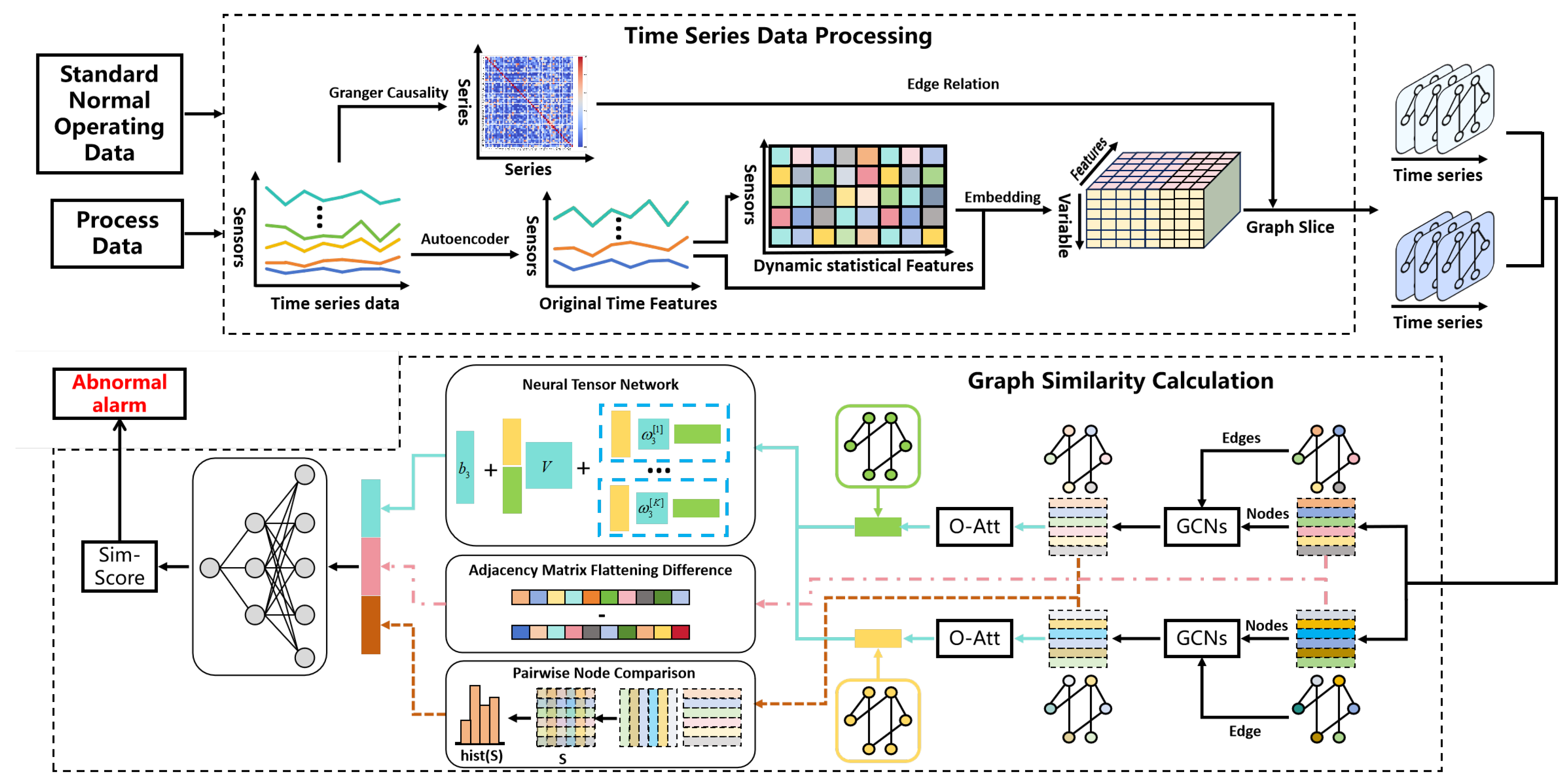
Figure 2.
Multi-dimensional time-varying feature graph embedding
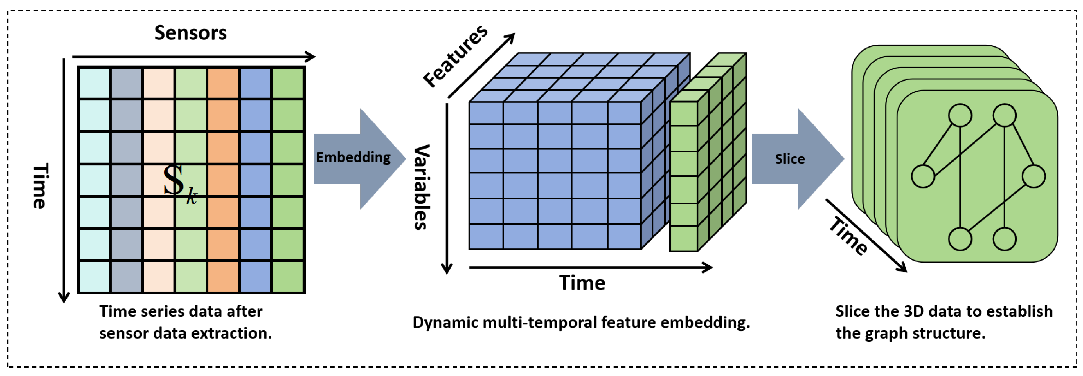
Figure 3.
Schematic diagram of the graph similarity calculation process
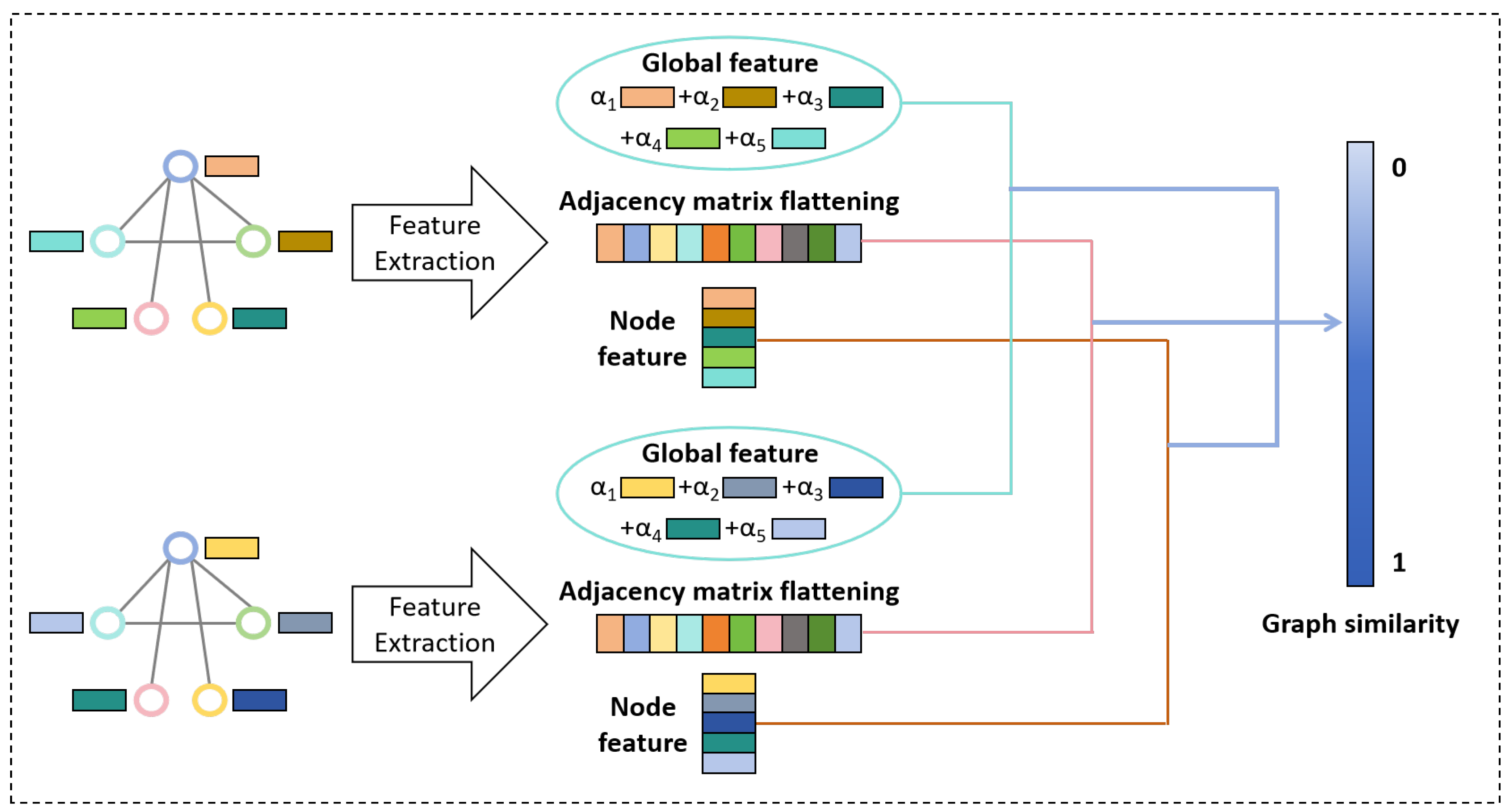
Figure 5.
Results of Granger causality calculation for TE process variables
Figure 6.
Autoencoder dimensionality reduction of TE process sensor data
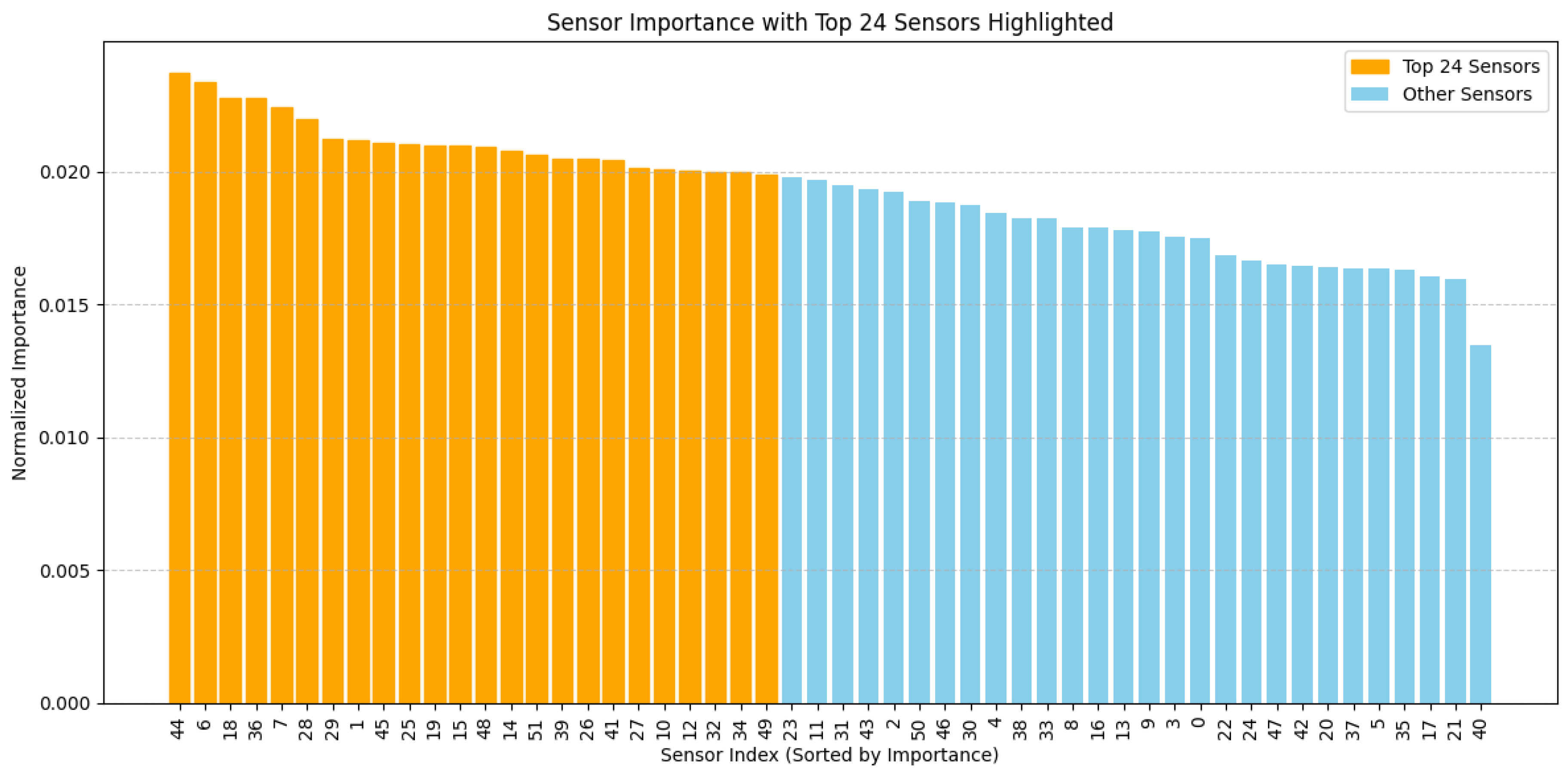
Figure 7.
Graph structure creation
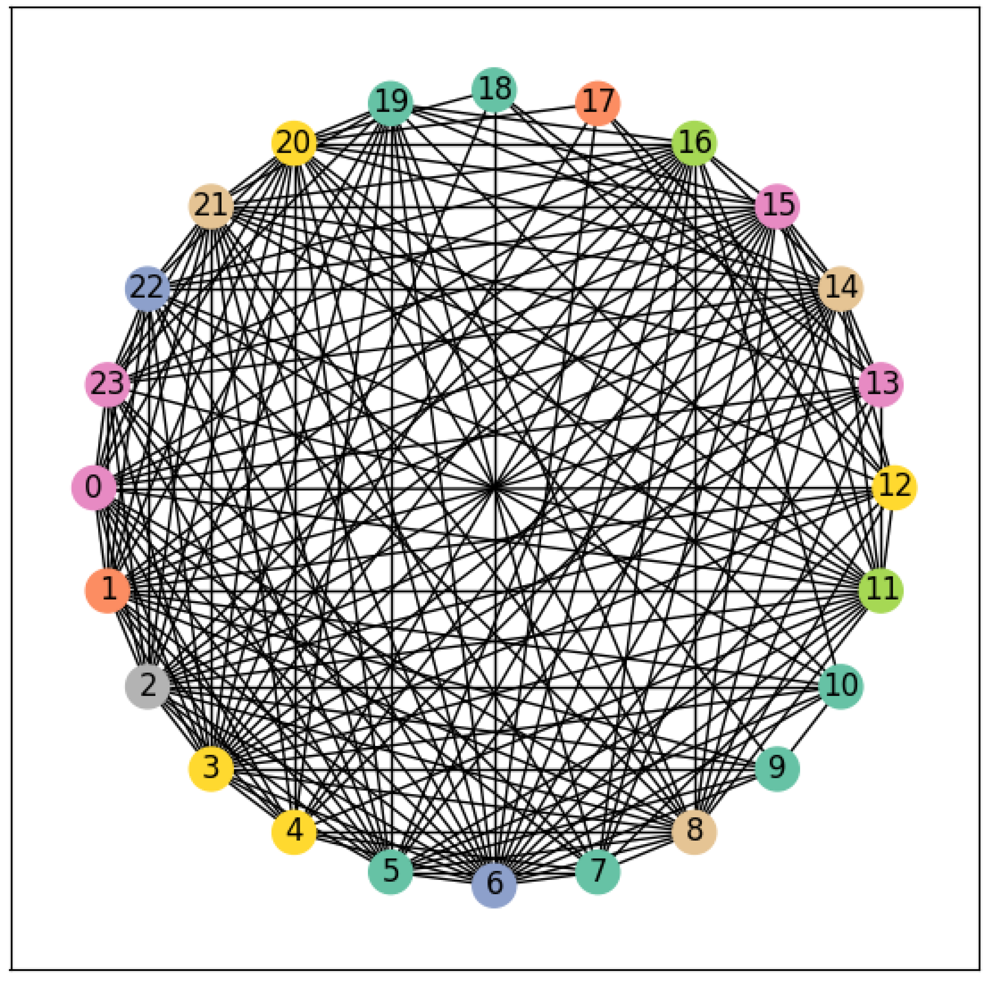
Figure 8.
Loss Curve
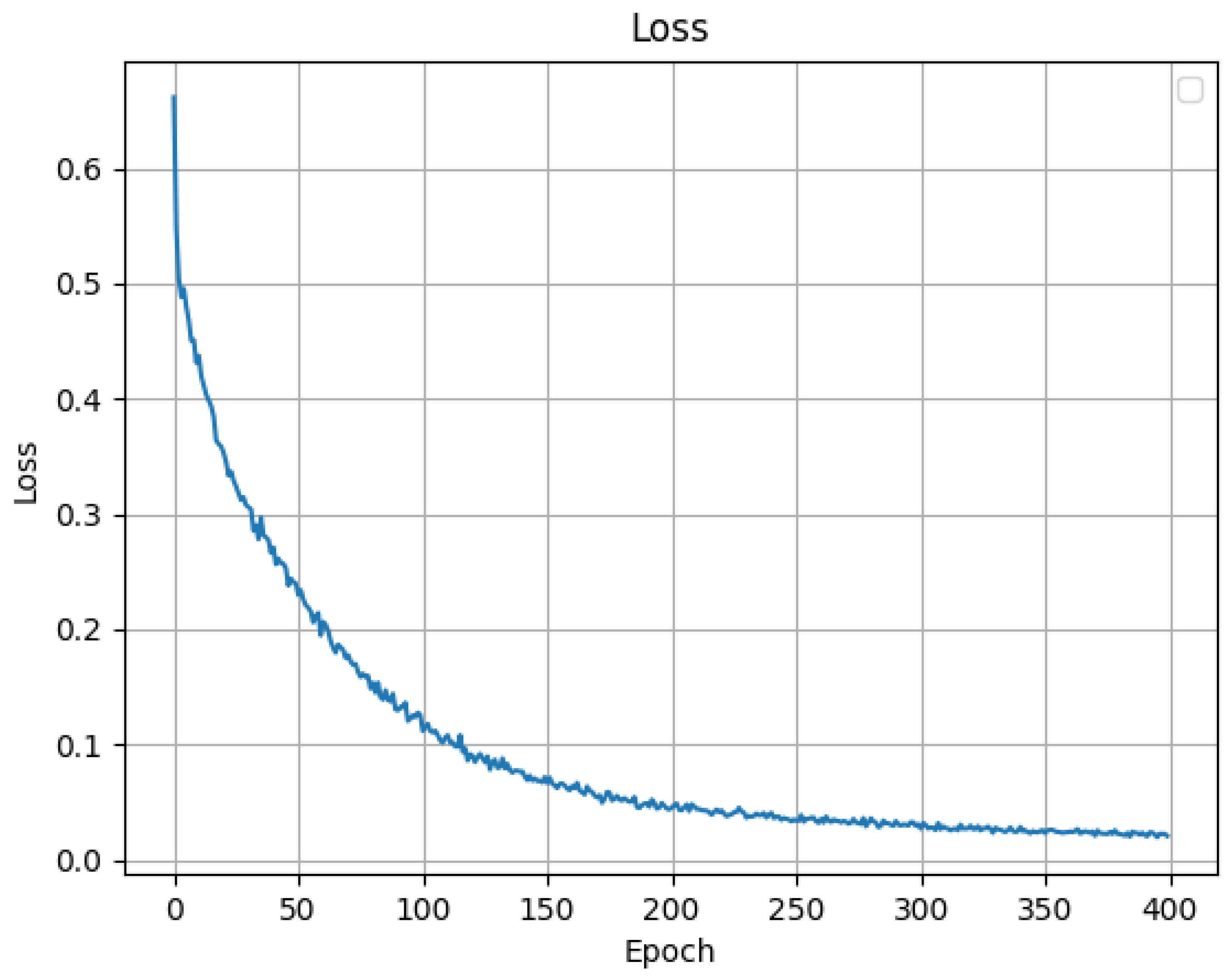
Figure 9.
Experimental results of abnormal monitoring for standard fault condition 01
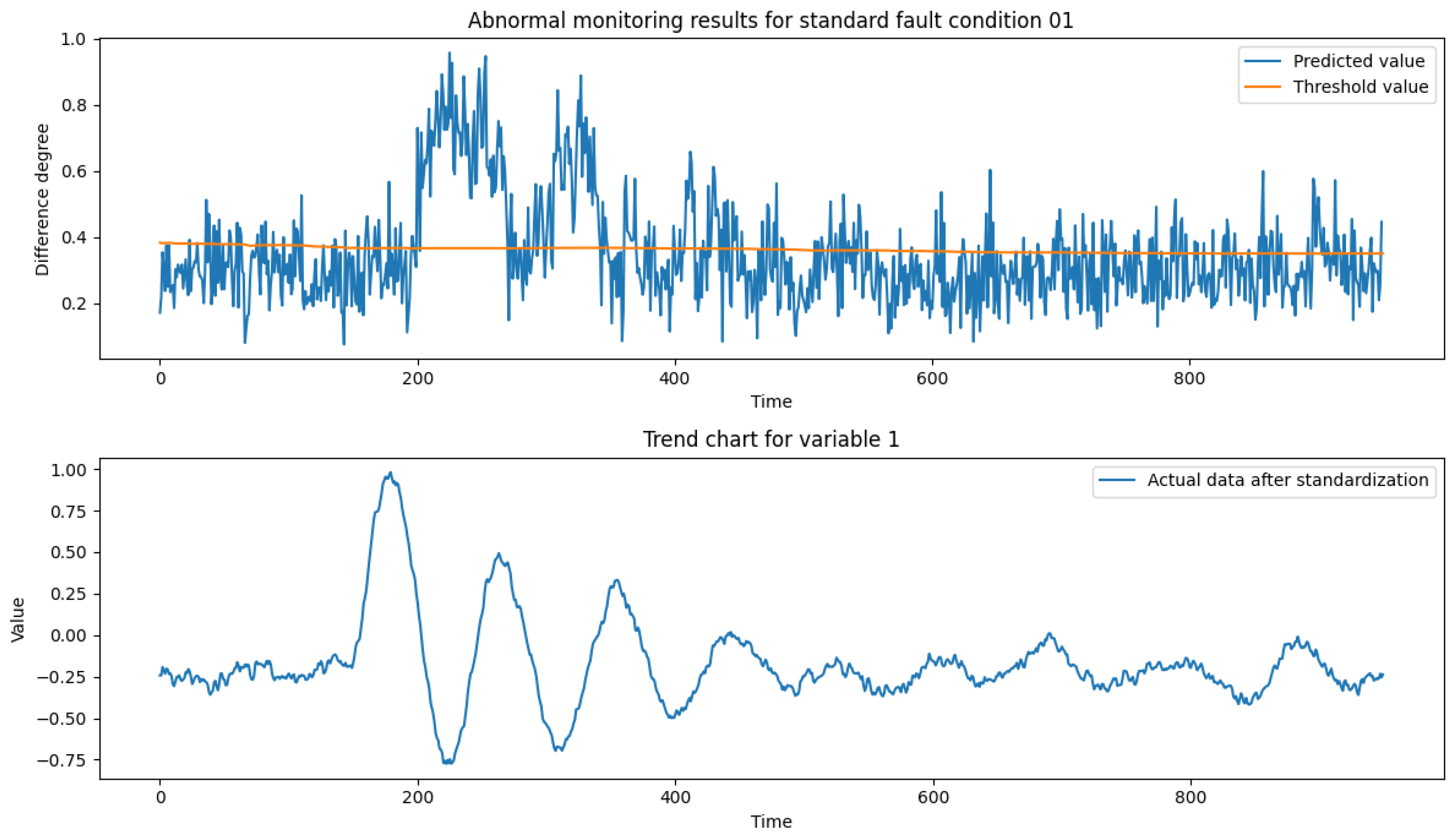
Figure 10.
Experimental results of abnormal monitoring for standard fault condition 06
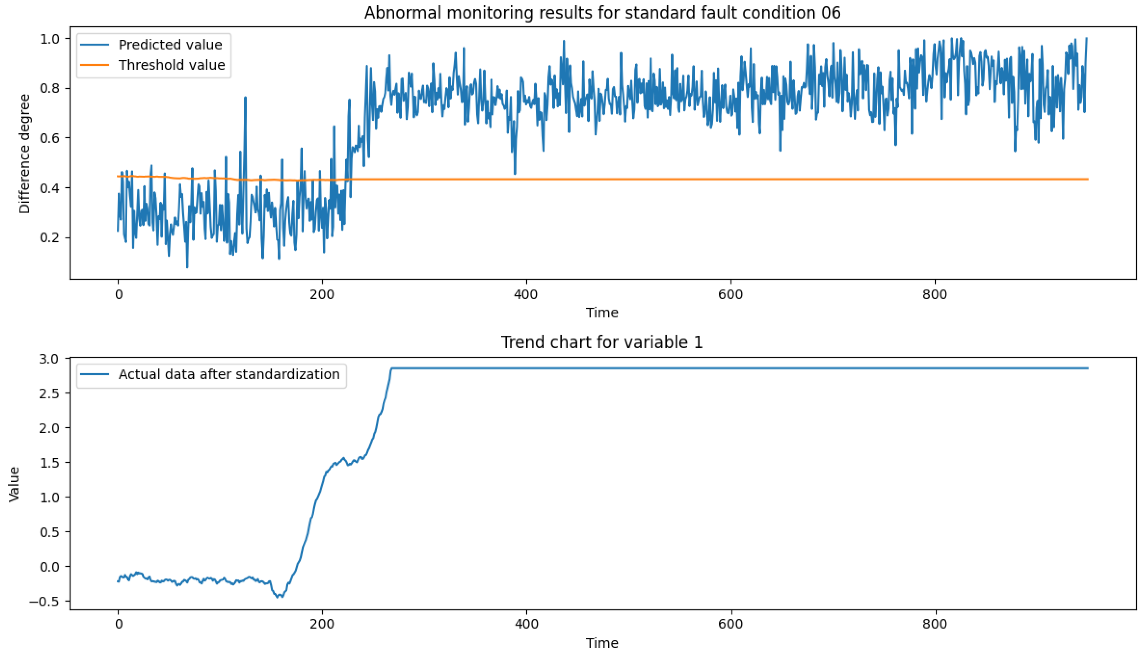
Figure 11.
Experimental results of abnormal monitoring for standard fault condition 13
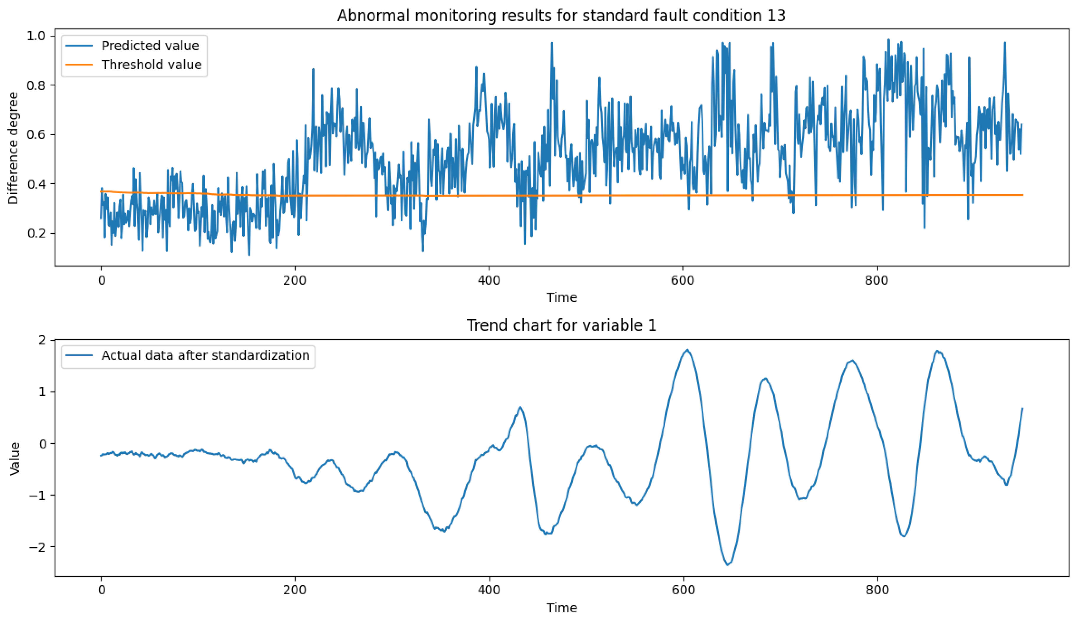
Figure 12.
Experimental results of abnormal monitoring for standard fault condition 18
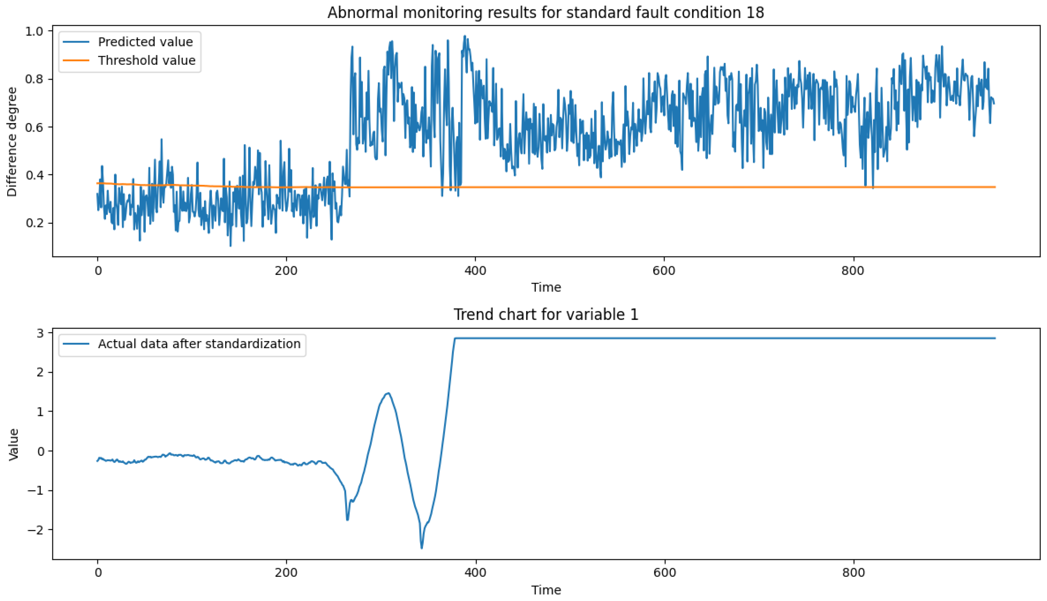
Figure 13.
Anomaly monitoring results based on cosine similarity
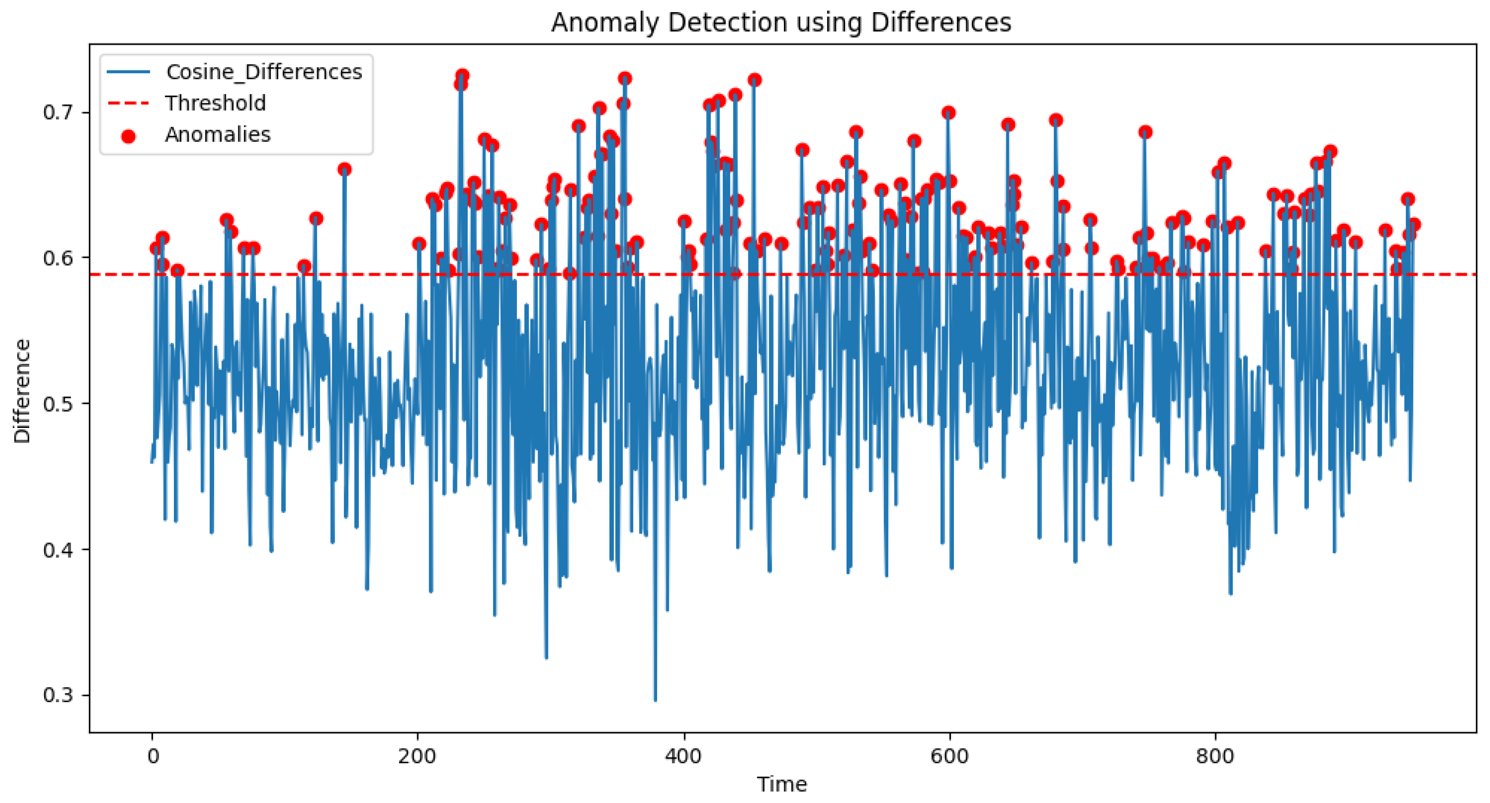
Figure 14.
PCA squared prediction error (SPE) anomaly monitoring results
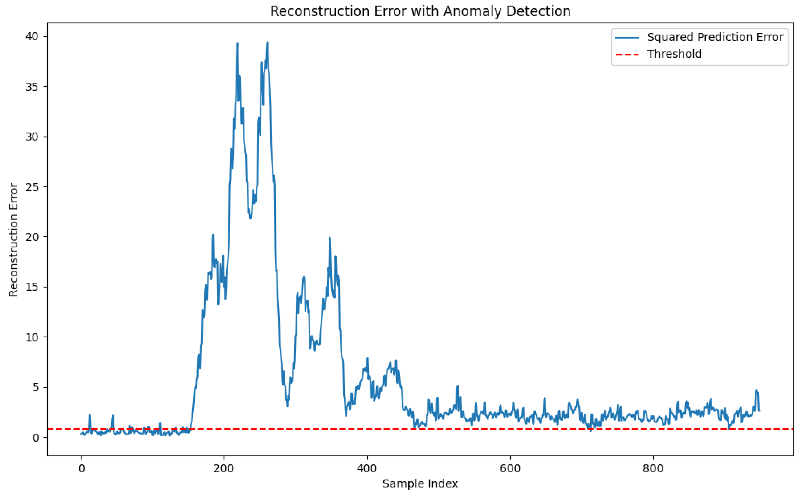

Table 1.
Results of the TE process autoencoder extraction of sensor variables, numbered in order of largest to smallest explained variance ratiot
Table 1.
Results of the TE process autoencoder extraction of sensor variables, numbered in order of largest to smallest explained variance ratiot
| Node number | Sensor number | Sensor Name |
|---|---|---|
| 0 | 44 | Total feed volume |
| 1 | 6 | Reactor pressure |
| 2 | 18 | Stripper Steam Flow |
| 3 | 36 | Product component D |
| 4 | 7 | Reactor level |
| 5 | 28 | Reactor feed component C |
| 6 | 29 | Empty material component A |
| 7 | 1 | Material D Flow |
| 8 | 45 | Compressor recirculation valve |
| 9 | 25 | Reactor feed component D |
| 10 | 19 | Compressor power |
| 11 | 15 | stripper pressure |
| 12 | 48 | Stripper gas flow |
| 13 | 14 | Stripper Level |
| 14 | 51 | Condenser cooling water flow |
| 15 | 39 | Product component G |
| 16 | 26 | Reactor feed component E |
| 17 | 41 | D feed volume |
| 18 | 27 | Reactor feed component F |
| 19 | 10 | Vapor/liquid separator temperature |
| 20 | 12 | Vapor/liquid separator pressure |
| 21 | 32 | Empty material component E |
| 22 | 34 | Empty material component G |
| 23 | 49 | Steam Valve for Stripper Tower |
Table 2.
Results of the third group of controlled experiments
| Methods | PCA | CNN | LSTM | Proposed model | ||||
| Index | FNR | FPR | FNR | FPR | FNR | FPR | FNR | FPR |
| Test1 | 0.1600 | 0.0050 | 0.0612 | 0.2000 | 0.0912 | 0.1067 | 0.0875 | 0.0867 |
| Test2 | 0.1867 | 0.0300 | 0.1638 | 0.1800 | 0.1288 | 0.1800 | 0.1163 | 0.1600 |
| Test3 | 0.2000 | 0.0625 | 0.1212 | 0.1800 | 0.1163 | 0.2067 | 0.1075 | 0.1600 |
Disclaimer/Publisher’s Note: The statements, opinions and data contained in all publications are solely those of the individual author(s) and contributor(s) and not of MDPI and/or the editor(s). MDPI and/or the editor(s) disclaim responsibility for any injury to people or property resulting from any ideas, methods, instructions or products referred to in the content. |
© 2025 by the authors. Licensee MDPI, Basel, Switzerland. This article is an open access article distributed under the terms and conditions of the Creative Commons Attribution (CC BY) license (http://creativecommons.org/licenses/by/4.0/).
Copyright: This open access article is published under a Creative Commons CC BY 4.0 license, which permit the free download, distribution, and reuse, provided that the author and preprint are cited in any reuse.


