
Submitted:
11 January 2025
Posted:
13 January 2025
You are already at the latest version
Abstract
The aim of this paper is to present an approach to condition monitoring of actuated mechanical systems (e.g. machine tools) operating in a steady state regime. The signals generated by the sensors placed on a mechanical system (e.g. a lathe gearbox) operating in a steady state regime are mainly a sum of many periodic components with different amplitudes and frequencies, sometimes mixed with a considerable amount of noise. Each periodic component (consisting of a fundamental sine wave and some harmonics) usually characterizes the state of a rotating part (e.g. a shaft, a belt, a bearing, etc.). This paper proposes a simple pattern extraction (recognition) method to find the time-domain description for the significant periodic components within these signals. This method is based on the averaging of a number of periodically selected signal samples. It acts as a kind of numerical multiple narrow bands pass numerical filtering. Some results prove the availability of this method for condition monitoring, applied in this work on three different signals: the active electrical power absorbed by an asynchronous AC electric motor that acts a lathe headstock gearbox, vibration of this gearbox and instantaneous angular speed of the output spindle.
Keywords:
sensors
; state signals
; mechanical system
; gearbox
; signal pattern recognition
; condition monitoring
1. Introduction
A reasonable assumption in monitoring and diagnosis is that a mechanically actuated system (machine) running in steady-state operation regime, containing mechanical components (MC, such as shafts, gears, belts, bearings, etc.) with periodic (usually rotary) motion, all together generate a state signal (e.g., vibration, mechanical power, force, torque, speed, etc.) to which all MC additively contribute, depending on their state. This state signal contains (usually) constant or slowly varying signal components (CSC) and periodically varying signal components (PVSC), where each CSC and PVSC is usually generated by one MC. The description of the health of the MC (its state) can obviously be done by analyzing the time-domain representation of the CSC and PVSC generated by MC. Because the mechanical system naturally mixes all these components into a single state signal, the first problem to solve for monitoring purposes is to separate the CSC and PVSC components generated by each MC from this signal. Of course, at the current state of the art, the CSC components cannot be separated because they have no characteristic elements that link them to the MC. It is obvious that any PVSC generated in the steady state regime can be approximated as a sum of harmonically correlated sinusoids (with a fundamental and several harmonics). The separation of any PVSC from the state signal is possible because there is a certain feature that links it to MC during a steady state regime of operation: the frequency (or the period T as well) of the fundamental component of the PVSC is equal to the rotational frequency (period) of the MC.
The separating of a PVSC is not always easy. For various reasons, the three characteristics of the fundamental and harmonic components within a PVSC as sine waves (amplitude, frequency and phase at the origin of time) can be constant, slightly variable or severely variable (especially with respect to amplitude). In some situations the PVSCs may be generated only temporarily, for short periods of time. For each of the three situations, synthetic or analytical techniques and methods for a partial or a complete description of the PVSCs exist in the literature.
The best-known technique is the Fast Fourier Transform (FFT) of the state signal, which is used in situations where frequencies and amplitudes are constant or vary very little [1,2] and the result is provided as a spectrum. A conversion from the time domain to the frequency domain is performed. Each peak in the spectrum describes the average values of the amplitude and frequency of a component in the PVSC (a fundamental or one of its harmonics). All components of all PVSCs are described in the FFT spectrum. The separation of the spectral peaks describing a certain PVSC generated by a certain MC must be done by other procedures. The FFT technique was applied in various situations for rotary machine monitoring and diagnosis [3,4,5,6,7].
When the PVSC characteristics vary greatly with time or especially when the PVSC is generated temporarily, an alternative to the FFT, the wavelet transform, can be used [8, 9, 10, 11and 12]. It is systematically applied in various fields, in particular to analyze state signals for monitoring purposes of rotary machines [4,5,6,7,8,9,10,11,12,13,14].
A natural question arises about the steady-state regimes: what exactly does this separation of a particular PVSC from a status signal mean? It just means that we should somehow get the time-domain representation of only this PVSC. The simplest way to obtain this representation is to filter the variable part of the status signal (converted to numeric format) with a tunable numerical multiple narrow band pass filter [15] having the pass frequencies harmonically correlated on 1/T Hz, 2/T Hz, 3/T Hz and so on (until the Nyquist limit) and keeping the original phases at the origin of time. The time-domain representation of the desired PVSC (found by using an appropriate value of T in the filtering, T being the period of the fundamental component of the PVSC) appears at the filter output. Indirectly, this is the technique used in this paper. This approach (and FFT as well) is correct only when any two or more harmonics of fundamentals of different PVSC do have not the same frequency.
For comparison and analysis purposes, it is easier to consider a time-domain representation of a PVSC (as a periodic signal) replaced with a PVSC pattern described by a single period obtained by appropriate averaging of the PVSC. This approach also covers the situation where the PVSC contains slightly varying sinusoidal components (caused, for example, by a slightly variation of MC speed). This is a short conceptual description of the approach in this paper.
Finding periodic patterns in state signals (especially vibrations) has been the subject of numerous previous theoretical and experimental approaches in signal processing techniques, particularly in the field of fault detection in rotating machinery. Cepstrum technique [16,17] (or the inverse Fourier transform applied to the logarithm of the magnitudes of the power spectrum obtained by the direct Fourier transform of status signal) or techniques derived from it have been applied in [12,18,19,20]. Spectral correlation density [21] (which examines the correlation between different components of a signal that are related to each other by frequency) or techniques derived from it was applied in [22,23,24,25]. Some other appropriate techniques (as cyclostationary analysis [26,27], autocorrelation [28,29] and averaged cyclic periodogram [30]) are also available.
A relative new approach in determination of patterns within the evolution of state signals (the well-known concept of signal pattern recognition) is a well-covered theoretical and experimental research topic [31,32].
Signal pattern recognition is a field of machine learning [33,34] (including deep learning based on neural networks [35]) that focuses on defining appropriate algorithms for automatically finding patterns in signals. It is associated with computer-based signal processing, achieved using artificial intelligence. The signal pattern recognition is used frequently for finding of abnormal working conditions (mechanical faults detection). Some interesting achievements on this topic in rotary machines are presented in [36,37] (on rolling bearings condition), [38,39,40] (on gears condition), [41] (on rotors vibrations), [12,42,43] (on induction motors condition), [44] (on driving belts condition, a topic also covered in our paper) and [45,46,47] (on detection of chatter in cutting processes).
Generally, vibration description signals are analyzed, but other resources are also used, such as force description signals [48], instantaneous angular velocity [47], active electric power [49], and electric current [50].
This diversity of approaches and achievements does not limit the perspectives of possible new contributions. There are still enough new accessible resources that can be highlighted and exploited in the identification of PVSC patterns useful for off-line monitoring and predictive diagnostics of mechanical systems (e.g., rotating machines) operating in steady state regimes. This is the objective of the present work, which proposes a simple method (with theoretical and experimental approaches) for extracting these PVSC patterns through a selective averaging process of the state signal samples (with examples in active electrical power, vibrations, instantaneous angular velocity) describing the operation of a lathe gearbox running in steady state regime. A setup and a theoretical approach already presented and described in [3] will be extensively used here for experimental purposes.
The rest of the paper is organized as follows:
-Section 2 presents the materials and methods (mainly the averaging method of state signal samples used to define the PVSC patterns);
-Section 3 presents some experimental results (with the PVSC patterns detected in active electrical power, vibration and instantaneous angular velocity);
-Section 4 is reserved for discussion, with a brief review of the requirements of the averaging method, of the performances in pattern detection, with a summary of the advantages and shortcomings, and future research directions.
2. Materials and Methods
An analog signal s(t) provided by an appropriate sensor placed on a mechanical system running in steady state regime is usually described (after analog-to-digital conversion) by a sequence of p equidistant numerical samples (with a constant sampling time Δt between any two successive samples), with the kth sample written as s[k], taken at the time t = k·Δt.
Suppose this signal contains a periodic component with the constant period T (or with 1/T constant frequency), and it has at least m periods. The numerical description of this component over a period T (as a pattern) can be obtained (extracted) mathematically with a good approximation using an averaging method with samples selected at regular time intervals (AMSSRTI) from the signal s (as a signal pattern recognition method). This regular time interval is exactly the period T. With m big enough, the selection rule of these samples results from the definition of a sample sT[h] of this pattern, according to:
Here is the nearest whole number (integer) to x. If the ratio n=T/Δt is exactly a whole number and the signal s has at least p = m·n samples, then a sample sT[h] of this pattern is more easily written as:
According with Eq. (2), a sample sT[h] of this pattern is calculated as the average of m equidistant samples from signal s, more specifically as the average of these samples: s[h], s[h+n], s[h+2·n]….., s[h+m·n]. Because usually T/Δt is not a whole number, the description of a sample sT[h] of this pattern from Eq. (1) is more exact. However, the description from Eq. (2) can also be regarded as acceptable with n defined as , if n is sufficiently large.
The pattern sT can be artificially extended to m successive identical periods, thus realizing a description of the periodical component under consideration, with a signal sTe having also p samples, but with n sets of m identical samples, the hth set being described with a good approximation as:
This signal sTe can be viewed as being generated at the output of a tunable numerical multiple narrow band pass (TNMNBP) filter, at whose input the signal s is applied (and processed according with Eq. (3)). This filter has the pass frequencies on T/j Hz, with j=1, 2...., here being the Nyquist limit. First period from the signal sTe is identical with the pattern sT.
The dependence of transmittance by frequency for this TNMNBP filter is partially depicted (as a particular example) in Figure 1 (frequency range between 1 and 300 Hz)), as a result of a numerical simulation (in Matlab) with Δt = 1/50000 s, T=1/33 s, and m = 60. A numerical sine wave with amplitude of 1 and a frequency f in the frequency range is fed into the filter as signal s. The amplitude of the output signal sTe is equal to the transmittance at this frequency.
and m = 60).
As clearly is indicated on Figure 1, mainly the input signal components (sine waves) having T/j =j·33 Hz frequencies pass through the filter unaffected (with undiminished or canceled amplitudes). A zoomed-in detail on in area A is depicted in Figure 2 (centered on the pass band frequency of 198 = 6·33 Hz). It is clear that the transmittance is not ideal (because of the small lateral lobes), however this filter can be used acceptably for the extraction of periodic signal components, as the experimental results will show below.
It is intuitive that this filter does not introduce any phase shift. An illustration of the effectiveness of AMSSRTI can be realized as follows. The signal s is defined to be periodic, as a sum of harmonically correlated harmonic components (a fundamental of period T and several harmonics with period’s l·T) as follows (as example):
Here is consider Δt = 1/25,000 s and T=1s.
The AMSSRTI is used to extract the periodic pattern sT from the signal s, with m = 50, according to Eq. (2), because = 25,000. It is expected that the correct operation of the AMSSRTI should be confirmed by the perfect identity between the pattern sT and the first period of the signal s. This identity is confirmed if any difference s[k]-sT[k] = 0 (also called residual) for any k = 1÷n, or for any time t expressed as k·Δt.
If we plot how these residuals s[k]-sT[k] evolve over time k·Δt, we should get a line that coincides with the t-axis. Figure 3 shows the time-domain representation of the residuals over a period T=1s (this being the time duration of the pattern sT).
Figure 3 proves that this theoretical assumption (with the residuals represented as a line identical to t-axis) is not totally true, for unknown reasons. However the maximum peak-to-peak amplitude of the residuals (3·10-10) is extremely small, so it can be considered that the AMSSRTI (and TNMNBP filtering as well) works as presumed. This approach also confirms that the AMSSRTI and TNMNBP filter don’t introduce any phase shift.
It is obvious that the smallest peak-to-peak amplitude of the residuals (and the best result for AMSSRTI and TNMNBP filtering) is obtained when as already proved in Figure 3. And obviously, the biggest peak-to-peak amplitude of the residual (and the worst result for AMSSRTI and TNMNBP filtering) is obtained when = 0.5. Figure 4 shows the worst-case time-domain representation of the residuals (2.49 peak-to peak, curve 1) after the AMSSRTI of the signal from Eq. (4) with T=1 and Δt = 1/25,000.5 s when = 0.5.
= 0.5); Curve 2 - Δt=1/25,000.493 (with= 0.493); Curve 3 - Δt=1/25,000.507 (with = 0.493);.
However this peak-to-peak amplitude of the residual is not significant compared with the peak-to-peak amplitude of sT (1430.9). By comparison, on Figure 4 curve 2 depicts the time-domain representation of the residuals if Δt = 1/25,000.493 s and curve 3 depicts the residuals if Δt = 1/25,000.507 s. In both scenarios = 0.493, as consequence, the peak-to-peak amplitude of the residuals (curves 2 and 3) strongly decreases.
This worst-case =0.5 often happens because the value of T. This worst-case can be avoided by resampling the signal s (by changing Δt) in order to obtain = 0.
There is another way to illustrate the effectiveness of AMSSRTI (and TNMNBP filtering as well). Consider a random noise signal rn where each sample is generated as a random number in the interval [-5 ÷ 5]. A short sequence of this signal is depicted in Figure 5. Consider that this random noise signal is mixed with a periodical signal s (playing the role of a PVSC in this simulation) described as:
A period of this signal s (T=1/25 s) is depicted in Figure 6. Figure 7 shows the result of the addition of signals rn+s during a period T (both simulated signals having the same sampling times Δt=1/100,000 s).
Figure 8 shows the result of the extraction of the pattern sT of this signal s (as curve 2) extracted from the signal rn+s using AMSSRTI, with m=100 and T=1/25 s.
Because of high noise of rn, the AMSSRTI with m=100 produces a relative noisy description of the pattern sT. A better result is presented in Figure 9 which shows the superimposed signal s (curve 1) and pattern sT (curve 2) obtained by AMSSRTI with m = 500.
In the previous example, it was shown that a very large value of m is required to reasonably reduce the influence of noise. This may be seen as an argument against the effectiveness of AMSSRTI. However, this situation (related to the type and magnitude of the noise) is very rare in practice.
With the signal s acquired under experimental conditions, as delivered by a sensor placed on an actuated mechanical system operating in the steady state regime, a correct extraction of the pattern sT of a PVSC by AMSSRTI usually requires the use of Eq. (1).
We should mention that it is mandatory to know (or to find somehow) the most accurate value of the period T of PVSC. An obvious approach is available for determining the exact value of the period T. Knowing an approximate value of T, we can set an interval around this value. We systematically change the value of T in this interval until we obtain by AMSSRTI (Eq. (1)) a pattern sT with maximum peak-to-peak amplitude. Thus the correct sT pattern and the exact value of the period T are determined. The correctness of this approach was confirmed experimentally as will be shown later.
It should also be mentioned that if the signal s contains (for example) two periodic components (1, 2) with periods T1, T2, and if the i-th harmonic of component 1 has the same period as the j-th harmonic of component 2 (or T1/i=T2/j), then AMSSRTI will produce distorted results in the description of both patterns sT1 and sT2, these two harmonics will be incorrectly described as belonging to both patterns.
This method of extracting a periodic signal pattern has been partially presented and was the subject of some experimental research related by the PVSC pattern found in instantaneous active electrical power, as a characterization of a three-phase AC asynchronous motor running at idle [51] and related by the PVSC pattern found in the evolution of the roughness of a 2D surface manufacturing by milling with a ball nose end mill [52].
3. Results
An experimental setup already described in detail in [3] is used here (Figure 10 and Figure 11). As an electrically driven mechanical system (with a three-phase AC asynchronous motor), a lathe gearbox is used (with the kinematic scheme partially shown in Figure 11). In this approach, some different signals provided by appropriate sensors are useful for condition monitoring purposes during a steady state regime (at idle) of the lathe gearbox: the active electrical power (Pa) absorbed by the driving motor, the vibration signal (Vs) and the instantaneous angular speed (IAS) as signal Ias. The active electric power Pa is mathematically defined [3] based on the signals supplied by a voltage transformer (VT) and a current transformer (CT). The vibration signal Vs is provided by a vibration sensor (VS) [3]. The signal Ias involved in the description of the instantaneous angular speed (IAS) of the spindle is provided by an IAS sensor IASS placed in the jaw chuck of the spindle [3]. All signals are sampled using a numerical oscilloscope [3] connected to a computer. The signal processing was done in Matlab.
The establishment of each signal has been extensively explained in two previous papers ([3] for Pa, and Vs, [53] for Ias). The gearbox is running in steady state at idle (according to the gearing diagram depicted in Figure 11), the rotation speeds (experimentally revealed) are highlighted in red.
Next only the variable part of these signals (as Pav, Vs and Iasv) are considered experimentally to extract the patterns of the periodic signal components induced by the operation (with constant speed rotation) of the gearbox elements (in particular belts and shafts) using AMSSRTI, if possible (if these components exist and have a sufficiently high amplitude). These patterns are useful for characterizing the state of each of these elements (condition monitoring).
3.1. Some Results Obtained by Analyzing the Variable Part of the Active Electrical Power Signal Using AMSSRTI
Figure 12 shows the time-domain representation of Pa (curve 1), a long sequence of 200 s (with pa = 5,000,000 samples, Δt = 1/25,000 s, 12 bit resolution). To produce Pav signal (as sP signal) the constant and the very low frequency variable part of Pa were mathematically subtracted from Pa. This very low frequency variable part (curve 2) was obtained by low pass filtering of Pa (using numerical multiple moving average filters [54]). Since this filtering produces false values at the beginning and end of the filtered sequence (zones ZA and ZB in Figure 12), these zones are removed from Pav (so Pav is shorter than Pa, as having just pav = 4,984,501 samples).
The time-domain representation of Pav is shown in Figure 13, with a zoomed-in detail (with 1.5detail with 1.5 s duration) from the beginning, shown in the rectangle on the right. This is a first simple proof that Pav is a deterministic signal with a very low level of noise. In the time-domain representation of Pav, many signals are mixed, most of them generated by the parts of gearbox, as will be demonstrated below.
There is a second more reliable proof that the Pav signal is deterministic with a low level of noise: how the FFT spectrum of Pav appears, as described in Figure 14.
According to the study performed before [3], each of the labeled peaks (A ÷ E) indicates the frequency (inverse of period) and the average amplitude of the fundamental of the periodic components PVSC generated by the flat belt 1 (A), the flat belt 2 (B), the shaft II (C), the shaft III and the spindle (D), the shaft I (E). Some other significant peaks are harmonics of the fundamentals A ÷ E already presented. It should be noted that the peaks in the FFT spectrum describes the average amplitude and frequency of the periodic components. The frequency (and period as well) of some PVSC may vary slightly (here due to a slight variation of motor rotation speed).
The patterns of each of these periodic components (as sPTA ÷ sPTE) can be extracted from signal sP by AMSSRTI based on Eq. (1). There is a first way to confirm partially the availability of AMSSRTI, related by the average frequencies fPA ÷ fPE of peaks A ÷ E revealed in Figure 14, as already fixed before. For each marked peak in the FFT spectrum (e. g. for the periodic component A), with AMSSRTI applied at the maximum possible value of m (tending to mmax =) we search in a small frequency range centered on the value given in the FFT spectrum (e.g., fPA = 5.34 Hz) for the frequency (period, TPA=1/fA) at which the pattern (sPTA) has the maximum peak-to-peak amplitude. This is the mean value of the frequency of the respective component (fPA), determined indirectly by AMSSRTI, which is expected to be close to that already shown in the FFT spectrum. This hypothesis is fully confirmed with the results depicted in Table 1.
For a more understandable graphical representation, we propose a partial extension of the patterns sPTA ÷ sPTE, up to the duration of 5 periods of their fundamentals (as sPTAe5 ÷ sPTEe5 for the MC A), based on Eq. (3) rewritten (as example for the component A), as:
These extended patterns sPTAe5 ÷ sPTEe5 can be obtained by the extension of patterns sPTA ÷ sPTE computed for different numbers of samples (or time durations of the Pav signal) considered in the definition of m < mmax.
To show the repeatability of the extended patterns sPTAe5 ÷ sPTEe5, there is an interesting possibility: to superimpose each two extended patterns related to the same component (e. g. A), both calculated with AMSSRTI from sPTA ÷ sPTE, for the same m, the first pattern (e. g., as being sPTAe5a) calculated on the first half of the total number of Pav samples (from 1 to pav/2, for almost 100 s), the second pattern (e. g. as being sPTAe5b) calculated on the second half of Pav samples (from pav/2 to pav, also for almost 100 s).
Figure 15 shows the superimposed extended patterns sPTAe5a (curve 1, m = 530) and sPTAe5b (curve 2, m = 530) related by the periodical component generated by the flat belt 1. We found that the average frequency fPA (or period TPA= 1/fPA) to consider in AMSSRTI for each extended pattern (whose which produces maximum peak-to-peak amplitude of the pattern) is slightly different: fPAa = 5.3368 Hz for sPTAe5a and fPAb = 5.3414 Hz for sPTAe5b. The sample at the beginning of the Pav sequence from which the second extended pattern (sPTAe5b) has been deduced (in a first approach pav/2) is conveniently changed to obtain the most correct possible overlap of the two patterns.
It is obvious that both patterns are quite similar (the flat belt is relatively new), as an argument for the repeatability, for the availability of AMSSRTI in condition monitoring of this flat belt transmission. There are some minor differences (except for the average frequency/period): the behavior of the belt is slightly changed in time probably because of heating due to slippage. This variation of the active electrical power is a direct consequence of the variation of the mechanical power induced by the belt and therefore of the belt behavior. During one period of this pattern, there is full belt circulation on the pulleys. The variation of the active electrical (mechanical) power is caused by the variation of the belt properties (e.g., stiffness) and does not necessarily describes (in this case) a critical belt failure.
The analytical description of the patterns can be found by using the Curve Fitting Tool application from Matlab, as the sum of harmonically correlated sinusoidal components (sine waves). Figure 16 shows the sPTAe5b pattern (as curve 1), the pattern based on the analytical description as the addition of eight harmonically correlated sinusoidal components (as curve 2, an addition of a fundamental FPA and seven harmonics HPA1, HPA2,…HPA6 and HPA8) and the residuals (curve 3) as the difference between. These sinusoidal components are described in Table 2.
We should mention that a very complicated procedure for finding the shape of the extended pattern for the PVSC generated by the first flat belt has already been presented in a previous work [3].
There is another important argument for the correctness of the AMSSRTI approach. Let us take a sequence of Pav with the duration of 50 periods TPA (234,300 samples for 9.372 s) from its beginning (as sP50). Correspondingly, the exact value of the frequency fPA=5.33448 Hz and the extended pattern sPTAe50 were determined. In Figure 17, the FFT spectrum of the sequence sP50 (in the range 0-40 Hz) is marked as 1. The FFT spectrum of the signal sP1r50 resulting from the mathematical extraction of this extended pattern from the analyzed sequence (with a sample described as sP1r50[k] = sP50[k] - sPTAe50[k]) is marked as 2. It is evident that the fundamental A and its 6 harmonics (A1 ÷A6) have disappeared from the spectrum 2 as a result of the elimination of the extended pattern sPTAe50 from signal sP50. For any other area (except the blue peaks), the two spectra are identical (the spectrum 2 is perfectly superimposed on spectrum 1).
Similarly with Figure 15, Figure 18 shows the superimposed extended patterns sPTBe5a (curve 1, m = 935) and sPTBe5b (curve 2, m = 935) related with the periodical component generated by the flat belt 2. We found that the average frequency fPB (or period TPB = 1/fPB) to consider in AMSSRTI for each extended pattern (whose which produces maximum peak-to-peak amplitude of the pattern) is quite similar: fPBa = 9.45223 Hz for sPTBe5a and fPBb = 9.45981 Hz for sPTBe5b.
There are not very significant differences between the extended patterns, except for the peak-to-peak amplitude, which is most likely related to the increase in temperature. It should be noted, however, that the peak-to-peak amplitude of the variable component of the active electrical power induced by the flat belt 2 is much greater than that induced by the flat belt 1. Most likely, this belt is close to the breakage limit, as it is 35 years older than the first one.
An extended pattern sPTBe89 with 235.494 samples was generated (from a sequence of 89 periods TPB at the beginning of Pav, with m = 89 and the best approximation of the average value of the frequency fPB = 9.446896Hz in AMSSRTI). This pattern is downsized at first 234.300 samples, and renamed sPTBe89*. Now the sPTBe89* extended pattern has the same number of samples as the sequence sP50 and the extended pattern sPTAe50 (both previously used to generate Figure 17). It can be mathematically eliminated from sP1r50 signal, a new signal is obtained as sP2r50, with a sample described as sP2r50[k] = sP1r50[k] - sPTBe89*[k] = sP50[k] - sPTAe50[k] - sPTBe89*[k]. The downsizing of sPTBe89 until sPTBe89*[k] was necessary to perform the mathematical subtraction above.
In other words, this signal sP2r50[k] is described with 234,300 samples taken from the beginning of Pav (as sequence s50) but after removing from sequence sP50 the periodical component generated by first and second flat belt (sPTAe50[k] respectively sPTBe89*[k]). The result of this subtraction is highlighted in the FFT spectrum of signal sP2r50 (marked with 3 in Figure 19, an extension of the result from Figure 17).
It is clear that, in addition to the result and comments of Figure 17, the removal of the PVSC generated by the second flat belt also causes the disappearance of the peaks associated with this component (the fundamental B, and the harmonics B1, B2) from the FFT spectrum. Obviously, looking at Figure 19, the components B, and B2 do not disappear completely, but rather some peaks of the FFT spectrum are diminished (the peaks marked with the symbol *). There is a partial explanation for this shortcoming: the periodic component generated by this second flat belt changes its amplitude more strongly with time (compared to the first flat belt), as already seen in Figure 18.
It is expected that the removing of these extended patterns from a lengthier Pav signal sequence no longer produces the same results in the FFT spectrum, characterized by the complete disappearance of peaks.
Similarly with Figure 15 and Figure 18, Figure 20 shows the superimposed extended patterns sPTCe5a (curve 1, m = 1350) and sPTCe5b (curve 2, m = 1350) related with the periodical component generated by the shaft II. We found that the average frequency fPC (or period TPC = 1/fPC) to consider in AMSSRTI for each extended pattern (whose which produces maximum peak-to-peak amplitude of the pattern) is quite similar: fPCa = 13.75435 Hz for sPTCe5a and fPCb = 13.759 Hz for sPTCe5b. Except a small difference between peak-to-peak amplitudes, there is a very good coincidence between patterns.
Figure 21 shows the superimposed extended patterns sPTDe5a (curve 1, m = 1720) and sPTDe5b (curve 2, m = 1720) related with the periodical component generated by the shaft III and spindle. We found that the average frequency fPD (or period TPD = 1/fPD) to consider in AMSSRTI for each extended pattern (whose which produces maximum peak-to-peak amplitude of the pattern) is quite similar: fPDa = 17.37406 Hz for sPTDe5a and fPDb= 17.38745 Hz for sPTDe5b.
Since the two shafts (III and spindle) have theoretically the same rotational speeds (however, the second belt drive’s transmission ratio is not exactly 1, as indicated in Figure 11), the AMSSRTI cannot generate a pattern for each of them.
Figure 22 shows the superimposed extended patterns sPTEe5a (curve 1, m = 2130) and sPTEe5b (curve 2, m = 2130) related with the periodical component generated by the shaft I. The average frequency fPE (or period TPE = 1/fPE) to consider in AMSSRTI for each extended pattern (which produces maximum peak-to-peak amplitude of the pattern) is quite similar: fPEa = 21.5606 Hz for sPTEe5a and fPEb= 21.5781 Hz for sPTEe5b. A small changing in amplitude of the pattern sPTEe5b is evident.
The mechanical inertia of the gearbox affects the shape and the size of the extended patterns of the PVSC inside Pav. It is obvious that fPAa < fPAb (Figure 15), fPBa < fPBb (Figure 18)…. fPEa < fPEb (Figure 22). This is due to the increase of the motor speed (probably because the increase of the supply voltage frequency, and certainly because to the decrease of the internal friction due to lubrication).
3.2. Some Results Obtained by Analyzing Vibration Signal Using AMSSRTI
A similar analyze can be done directly on vibration signal Vs (written as signal sV). This signal was acquired during the same steady state regime as for active electrical power Pa previously studied (a sequence of 200 s, with pa = 5Ms –or 5,000,000 samples-, Δt = 1/25,000 s as sampling time) and depicted in Figure 23.
This signal Vs describes a beating phenomenon, explained and studied in detail in [55]. The shaft III and the spindle (both with mechanical unbalance) rotate at almost the same instantaneous angular speed, a beating phenomenon (with nodes and anti-nodes) occurs. There is a dominant vibration, shown in an enlarged detail on Figure 23 (on the right), with almost the same frequency as the rotation frequency of the spindle. The partial FFT spectrum of this signal (frequency range 0 ÷ 40 Hz) is shown in Figure 24. A zoomed section of this spectrum is shown in the middle, with the same frequency range and amplitude range severely diminished: 0 ÷ 4.2 mV.
It is surprising that in the FFT spectrum of the Vs signal, the same A ÷ E fundamentals of the PVSC are present as previously seen in the FFT spectrum of Pav (Figure 14). This means that the same phenomena are reflected in the time-domain representation of the active electrical power and vibration. Note that the fundamental A is described with diminished amplitude because it has a frequency below the natural frequency of the sensor (approx. 8 Hz). As expected, there is a dominant PVSC (with D as fundamental, 17 37 Hz frequency and 119.3 mV amplitude) with the origin already explained above (as detailed in Figure 23).
Even if the vibration description signal (Vs, as sV) contains the beat phenomenon and even if there is a large dominant VPSC (with D as fundamental), the patterns obtained by AMSSRTI are of interest for monitoring. Related by the behavior of first flat belt, Figure 25 shows the superimposed extended patterns sVTAe5a (curve 1, m = 533 for almost 2.5 Ms at the beginning of sV) and sVTAe5b (curve 2, m = 530 for almost next 2.5 Ms of sV). We found that the average frequency fVA (or period TVA= 1/fVA) to consider in AMSSRTI for each extended pattern (whose which produces maximum peak-to-peak amplitude of the pattern) is slightly different: fVAa = 5.33736 Hz for sVTAe5a and fVAb = 5.34151 Hz for sVTAe5b. As a first approach, since the two patterns appear to be strongly affected by noise, they are plotted in Figure 25 after a numerical low-pass filtering (using a moving average filter with 100 samples in the average). The sample at the beginning of the sV sequence from which the second extended pattern (sVTAe5b) has been deduced (almost pa/2) is conveniently changed to obtain the most correct possible overlap of the two patterns.
As can be seen on Figure 25, there are sufficient similarities between the two patterns (despite the relatively long durations between the sequences from which they were derived, almost 100 s) to prove the validity of this resource for describing the condition of the belt using AMSSRTI of vibration signal sV. It should be noted that in the patterns of this flat belt, the fundamental A has a low amplitude (due to the low sensitivity of the sensor at low frequency), but there are some harmonics with higher amplitudes. It is interesting to highlight the resources offered by the unfiltered time-domain representation of these two patterns, shown in Figure 26, where there are still obvious similarities between. We propose to realize the extension of one of the patterns (e.g., for unfiltered sVTAe5b) to several periods (e.g., 50 periods, with 234,000 samples), as sVTAe50b. The partial FFT spectrum of this pattern (in the range 0 ÷ 175 Hz) is shown in Figure 27. This figure also shows a zoomed-in detail of this partial spectrum (the same frequency range). This extension of the pattern was necessary to achieve high frequency resolution of the FFT spectrum.
First remark related by Figure 27: the appearance of the FFT spectrum proves that there is no noise in the extended pattern sVTAe50b (so neither in unfiltered sVTAe5a and sVTAe5b patterns). In addition, this signal is strictly deterministic, being defined as the sum of strictly harmonically correlated components with frequency spacing exactly equal to the value of fVAb.
This is another strong argument in favor of the usefulness of AMSSRTI for describing the state of a mechanical component of the mechanical system under investigation. The spectral content highlighted here in the case of the first belt vibration pattern was not observed in the case of the active electrical power pattern (Figure 26 compared to Figure 25) because this power is defined by numerical low pass filtering of the instantaneous power.
It is very important to note that, in the same way, for all the patterns presented above (in the time-domain representation of the variable part of the active electrical power) it is possible to characterize them by means of the FFT spectrum of the extended patterns. Both variants of the extended pattern (filtered and unfiltered) can be used to monitor the condition of a rotating MC. The filtered version has the advantage of a quick estimation of the condition (e.g., by comparison with a standard pattern).
Related by the behavior of second flat belt, Figure 28 shows the superimposed extended patterns sVTBe5a (curve 1, m = 935 for almost 2.5 Ms at the beginning of sV) and sVTBe5b (curve 2, m = 935 for almost next 2.5 Ms samples of sV). The average frequency fVB (or period TVB= 1/fVB) to consider in AMSSRTI for each extended pattern (which produces maximum peak-to-peak amplitude of the pattern) is again slightly different: fVBa = 9.4525 Hz for sVTAe5a and fVBb = 9.4596 Hz for sVTAe5b. Figure 29 shows the same extended patterns treated with numerical low-pass filtering, using a moving average filter (with 30 samples in the average).
There are certain similarities between the filtered patterns, but also differences, probably due to the change in temperature of the belt during operation. It should be noted that the flat belt 2 introduces greater peak-to-peak variation in the active electrical power pattern compared to flat belt 1 (see Figure 18 and Figure 15). In the description of pattern from vibration, the flat belt 2 introduces less variation than belt 1 (see Figure 29 and Figure 25).
Figure 30 shows the superimposed extended patterns generated by the shaft II: sVTCe5a (curve 1, m = 1365 for almost 2.5 Ms at the beginning of sV, with fVCa = 13.75399 Hz) and sVTCe5b (curve 2, m = 1365 for almost next 2.5 Ms samples of sV, with fVCb = 13.76565 Hz). Figure 31 shows the same extended patterns treated with numerical low-pass filtering, using a double moving average filter (with 37 and 50 samples in the average).
An examination can now be made of the components of one of the unfiltered patterns in Figure 30 (e.g., sVTCe5b). Using the Curve Fitting Tool application from Matlab, an approximation of this pattern has been identified based on the first two most representative sinusoidal components. This approximation -labeled sVTCe5b2c- is described as:
Figure 32 shows these two superimposed patterns: sVTCe5b pattern as curve 2 (already shown in Figure 30), and sVTCe5b2c as curve 3, mathematically described by Eq. (7).
A detail from zone ZA illustrating the fit of the two curves is magnified in region ZB.
As expected, the angular frequency of the first component, or fundamental (as ω1 = 86.57 rad/s), is related to the frequency fVCb (with 2·π·fVCb ≈ ω1, so 86.4921 rad/s≈ 86.57 rad/s). The AMSSRTI ensure that the second component of sVTCe5b2c from Eq. (7) (with angular frequency ω2= 4152 rad/s) is necessarily harmonically correlated with the fundamental. This is totally confirmed, because: ω2/ω1 = 47,9611 ≈ 48. This very small difference is explained by the approximations of the fitting procedure in finding the values of the constants from Eq. (7).
Obviously, this second component in Eq. (7) must correspond to a vibratory phenomenon. The most plausible explanation for the origin of this phenomenon is that in Figure 11, a 48-toothed gearwheel is mounted on shaft II in free meshing (not transmitting mechanical power). The second component in Eq. (7) is generated by the meshing sequence of the teeth of this wheel as a vibration-generating phenomenon with a frequency 48 times higher than the rotational frequency of the shaft II.
It is clear that this second component of Eq. (7) is always present in the vibration signal sV. Moreover, it should be emphasized by AMSSRTI applied to signal sV, related by a variable component with period TVC48=TVC/48. The extended pattern of this component on five periods TVC48 (as sVTC48e5a pattern) is shown as curve 1 in Figure 33 (m = 3250, on first 4.94 s of the signal sV, with the best approximation of the frequency at this variable component fVC48a = 660.045986 Hz). The same analysis by AMSSRTI was performed on a new sV signal sequence starting at the 100th second (m = 3250 with the best approximation of the frequency at this variable component fVC48b = 660.53362 Hz). An extended pattern (sVTC48e5b) was generated, represented by curve 2 in Figure 33 (moved appropriately to get the best overlap with curve 1). The similarity of these patterns is more than obvious, even though they are described with a small number of samples (190).
Similarly, AMSSRTI can be used to determine if there is a variable component induced by the 58 -toothed gearwheel placed on shaft II, as a toothed wheel that transmits mechanical power. The extended pattern of this component on five periods TVC58 (as sVTC58e5a pattern) is shown as curve 1 in Figure 34 (m = 3250, on first 4.04 s of the signal sV, with the best approximation of the frequency at this variable component fVC58a = 797.5646 Hz ≈ 58· fVCa = 58·13.75399 Hz = 797.73142 Hz). A new extended pattern of this component on five periods TVC58 (as sVTC58e5b pattern) is shown as curve 2 in Figure 34 (m = 3250, on 4.04 s of the signal sV, starting with the 100th second, with the best approximation of the frequency at this variable component fVC58b = 798.1551Hz ≈ 58· fVCb = 58·13.76565 Hz = 798.4077 Hz).
Again, a good similarity of the two patterns from Figure 34 (each of them described with 155 samples) was obtained. This proves that the vibrations induced by this toothed wheel occur systematically, and that the AMSSRTI is obviously a good option in gearbox condition research. Increasing the sampling rate of the signal sV increases the number of samples of the patterns from Figure 33 and Figure 34.
As the speed of the electromotor driving the gearbox increases slightly over time (due to the decrease of mechanical load, through the effect of the viscosity decreasing of the lubricating oil), all the frequencies of the components studied so far increase slightly over time. Therefore it should be mentioned that the shape of the patterns generated by AMSSRTI depends relatively strong on the value of m, especially in the case of high frequency components (e.g., for TVC48 periodic component with the patterns already shown in Figure 33 for m = 3250). Figure 35 reproduces these two patterns (curves 1 and 2) but also the extended patterns resulting from AMSSRTI with the maximum possible value for m (curves 3 and 4).
Figure 36 shows the superimposed extended patterns generated by the shaft I, for m = 2155, as sVTDe5a (curve 1, for almost 2.5 Ms at the beginning of sV, with fVDa = 21.56087 Hz) and sVTDe5b (curve 2, for almost the next 2.5 Ms samples of sV, with fVDb = 21.57886 Hz). Figure 37 shows the same extended patterns treated with numerical low-pass filtering, using a moving average filter (with 30 samples in the average). It should be noted that the two filtered extended patterns derived from the vibration analysis by AMSSRTI are more similar for this shaft than for any flat belt previously presented (belt 1 in Figure 25 and belt 2 in Figure 29). Similar studies can be performed on the periodic components associated with the rotation of the shaft I and spindle.
3.3. Some Results Obtained by Analyzing Instantaneous Angular Speed Using AMSSRTI
An instantaneous angular speed (IAS) sensor (as IASS) was placed in the jaw chuck of the spindle (Figure 10 and Figure 11). This sensor is actually a stepper motor that plays the role of a two-phase, 50-pole AC generator [53]. At relatively high IAS, this sensor generates two AC signals (equal amplitudes, 90 degrees out of phase) with 50 periods per revolution. These signals are processed appropriately in order to produce IAS, at the same sampling rate, using an interesting approach, presented in [56]. This approach is based on determining the angle of rotation of the sensor rotor and the numerical derivative of this angle with respect to time. The time-domain representation of the IAS during an identical steady state regime considered previously (but shorter, with duration of only 10 s and a sampling rate of 100,000 s-1) is shown in Figure 38.
A detail from zone ZA, at the beginning of IAS (with 587 samples, during 5.87 ms) is shown magnified in zone ZB. A significant variability of the IAS signal is observed (as peak-to-peak amplitude, with a maximum value of 18.87 rad/s) around the mean value of 109.47 rad/s, corresponding to a mean rotation frequency of 109.47/2/π=17.4227 Hz. This high variability is due to the fact that this AC generator has mechanical and electrical design imperfections and introduces a variable component related to these imperfections, which is greatly amplified by numerical derivation.
The fundamental frequency (period) of this variable component is equal to the rotational frequency (period) of the spindle. In order to use AMSSRTI properly (here with a smaller allowed values for m, because the IAS sequence is short), this variable component should be removed somehow, e.g., using a moving average filter with the number of samples in the average equal to the number of samples per spindle rotation period (here 5,739 samples). This means that the AMSSRTI pattern generated by the spindle cannot be obtained. Figure 39 shows the variable part of the filtered IAS, seen from here onwards as signal sI.
Of course, all other components of the signal sI are affected by this filtering (some with diminished amplitude, others being eliminated). However, some of them can still be revealed by AMSSRTI.
Figure 40 shows the partial FFT spectrum of the signal sI (0÷40 Hz range, with 0.100715 Hz resolution).
Surprisingly, this spectrum contains the four fundamental (A, B, C and E) and some harmonics (B1, B2, C1) of the PVSCs previously highlighted in the active electrical power spectrum (Figure 14) and vibration description signal spectrum (Figure 24). This is the first important argument in favor of using the signal sI in condition monitoring using AMSSRTI. As clearly indicated, the fundamental of PVSC generated by the rotation of spindle in signal sI (D in Figure 14 and Figure 24) was completely eliminated in the spectrum from Figure 40 by due to an appropriate filtering of IAS signal.
In the same way as above, AMSSRTI can be used in signal processing of the signal sI to extract the extended patterns of these available variable components.
Related by the behavior of first flat belt mirrored in filtered signal sI (with fundamental A in Figure 40), Figure 41 shows the superimposed AMSSRTI extended unfiltered patterns sITAe5a (curve 1, m = 25 on 467,075 samples at the beginning of sI) and sITAe5b (curve 2, m = 25 for next 467,800 samples of sI). The average frequency fIA is slightly different for each pattern: fIAa = 5.40021 Hz for sITAe5a and fIAb = 5.4107 Hz for sITAe5b.
As expected, there is a good match between the two extended patterns. Surprisingly, the sI signal variation induced by belt 1 is detected and described by the IAS sensor (via AMSSRTI), even if this sensor is placed far away from this belt.
A detail in zone ZA on Figure 41 is magnified in zone ZB. One can see here (especially with respect to the pattern sITAe5a) the existence of a variable signal component, the origin of which will be explained later in the discussion about Figure 42 and Figure 43.
Related by the behavior of second flat belt mirrored in sI (having the fundamental B in Figure 40), Figure 42 shows the superimposed extended unfiltered patterns sITBe5a (curve 1, m = 46 on 484,702 samples at the beginning of sI) and sITBe5b (curve 2, m = 46 for next 484,702 samples of sI). The average value of the frequency used in the AMSSRTI was fIBa = 9.48999 Hz and fIBb = 9.49061 Hz.
A detail from zone ZA (with 370 samples, during 3.7 ms) is shown magnified in zone ZB. This is an example of a distortion phenomenon of the AMSSRTI patterns (more evident in sITBe5a compared with sITBe5b), already anticipated in before in Section 2 of this paper.
It should be noted that the PVSC generated by the spindle in the signal sI has not been completely removed by the IAS filtering (only the D fundamental has been completely removed, as Figure 40 shows that it is missing), some of its upper harmonics still remains in the signal sI. It was found that the period of the 369th harmonic of the fundamental of the variable component generated by the second belt (as TIBa369 = TIBa/369 or TIBb369=TIBb/369) is practically equal to the period of the 201st harmonic of the fundamental of the PVSC generated by the shaft (as TIDa201 =TIDa/201 or TIDb201 =TIDb/201), in other words 369·fIBa ≈201·fIda ≈ 3501.80 Hz or 369·fIBb ≈201·fIDb ≈ 3502.035 Hz. For this reason, the sinusoidal component with period TIDa201 (or TIDb201) appears in the extended AMSSRTI pattern sITBe5a (or sITBe5b) as false sinusoidal component TIBa369 (or TIBb369). Also in these AMSSRTI extended patterns appears any other sinusoidal component having the period TIDa201/j ≈ TIBa369/j (or TIDb201/j ≈ TIBb369/j).
Of course, it is possible to find the AMSSRTI extended patterns sITB369e5a and sITB369e5b of the false variable component with the fundamental with very small period TIBa369 and TIBa369 (or high frequencies as well). These extended patterns (having 145 samples) were each one determined on almost half of number of samples (495,900) from signal sI (for m=17,100) and shown in Figure 43.
As can be clearly seen in Figure 43, there are some similarities between these patterns (as shapes not as amplitudes), already found earlier in Figure 42 as shown in region B. We discovered that these false signal variable components TIDa201 and TIDb201 also occur in the sITAe5a and sITAe5b extended patterns already revealed in Figure 41 (highlighted in the region ZB), as having TIAa648 (or TIAb648) as periods of the fundamental A.
Related by the behavior of shaft II mirrored in signal sI (with fundamental C in Figure 40), Figure 44 shows the superimposed AMSSRTI extended unfiltered patterns sITCe5a (curve 1, m = 68 on 491,776 samples at the beginning of sI) and sITCe5b (curve 2, m = 68 for next 491,776 samples of signal sI). The average value of the frequency used in the AMSSRTI was fICa = 13.826942 Hz and fICb = 13.79066 Hz. Since there are ten periods on each extended pattern, it is obvious that the amplitude of the first harmonic (having period TICa1 or TICb1 described in Figure 40 with the peak C1) is much bigger than the fundamental (having the period TICa or TICb).
Related by the behavior of shaft I mirrored in signal sI (with fundamental E in Figure 40), Figure 45 shows the superimposed AMSSRTI extended unfiltered patterns sITEe5a (curve 1, m = 106 on 489,720 samples at the beginning of sI) and sITEe5b (curve 2, m = 106 for next 489,720 samples of sI).
The average value of the frequency used in the AMSSRTI was fIEa = 21.6422 Hz and fIEb = 21.64315 Hz. In Figure 44 and Figure 45, false variable components also appear, as described earlier. Eliminating these false variable components in the AMSSRTI patterns requires a simple approach, such as determining their mathematical description (by curve fitting, as was done earlier in Figure 16) and removing them from the AMSSRTI.
The AMSSRTI can be used to process state signals produced by many other types of sensors describing a steady state regime or a working process (e. g. in milling process).
4. Discussion
The facilities of numerical description and sampling of the signal sequences generated by the sensors (such as resolution, sampling rate, number of samples), as well as the facilities for assisted computation, allow their processing by various relatively simple numerical techniques and methods.
Among these techniques, this paper proposes the AMSSRTI as procedure for determining the pattern of any periodically varying signal component (PVSC) produced in a steady-state regime of a driven mechanical system, which yields interesting experimentally results for three different signals: active electric power, vibration and instantaneous angular velocity. These signals were provided by appropriate sensors placed on a lathe gearbox headstock (different sensors placed in different locations). The patterns found in these signals characterize the functioning (correct or wrong) of mechanical components of the mechanical system in steady state motion regime (with constant speed rotation) and are useful for offline monitoring of their condition.
4.1. A Brief Overview of the Requirements for Obtaining AMSS Patterns
Mainly some computer programs conceived by us and only occasionally an application in Matlab (Curve fitting tool) were used to prepare and to apply the AMSSRTI (as averaging method with m samples selected at regular time intervals). To find an AMSSRTI pattern of any PVSC inside the state signal (based on Eq. (1)), or any AMSSRTI extended pattern (based on Eq. (3)) is necessary to know:
-The variable part of the state signal.
-The exact value of sampling time (sampling interval) Δt of the numerical description of the state signal (as being constant).
-The number of samples of this signal.
-The exact value of period T (or frequency) of the PVSC.
-The number of time intervals conveniently chosen (m) preferably as larger as possible.
The most difficult issue in the application of AMSSRTI is the determination of the exact value of the period T (or frequency) of the PVSC. In our approach, we have defined and validated an efficient method: in a chosen (small) range for the period (frequency) value, we search for the value at which the peak-to-peak amplitude of the resulting AMSSRTI pattern is maximal. The range is centered on the approximate value of the period (frequency) of the PVSC given by the FFT spectrum or by the kinematic scheme of the actuated mechanical system. After each search result, the range is narrowed and the search is repeated a sufficient number of times to obtain the most accurate value of the period (frequency).
The efficiency of this method of exact determination of the period (frequency), systematically used in this paper, can be demonstrated comparatively, as shown in Figure 46. In the case of the variable component of the active electric power induced by the first flat belt (Figure 15), the AMSSRTI extended pattern sPTAe5a was found (as curve 1, for m = 530, for which the exact frequency fPAa = 5.33748 Hz was determined). This extended pattern is redrawn identically as curve 1 here below in Figure 46.
In the same figure, curve 2 shows an extended pattern (as sPTAe5a-) under the same condition but with an intentionally imprecise, very slightly lower frequency (as fPAa- = 5.335 Hz), curve 3 shows this extended pattern (as sPTAe5a+) but with an intentionally imprecise, very slightly higher frequency (as fPAa+ = 5.339 Hz). The difference between the extended patterns is obvious (also favored by the large value of m), despite the very small changes of frequency. It is obvious that the extended pattern 1, corresponding to the exact frequency, has the largest peak-to-peak amplitude and more accurately describes the behavior of the flat belt 1.
It is important to note that even in the absence of an approximate period (frequency) value of a variable periodic component it is possible to use AMSSRTI, starting with a sufficiently large frequency range. The value of period (frequency) for a possible periodic variable component is found to be the period (frequency) that produces a pattern with the largest peak-to-peak amplitude.
When two patterns (or extended patterns as well) with obvious similarities that characterize the same variable signal component (at different time instants) are to be compared (by overlapping, e.g., Figures 15, 18, 20, etc.), one of them is taken as the reference and the other is shifted until the best overlap is achieved. Shifting is accomplished by changing the first sample of the state signal used in the pattern construction. Any offset component (or DC bias as well) of the pattern should be eliminated.
If the two patterns have relatively large differences in shape, for a correct overlapping, the first sample used in each pattern construction is shifted so that each pattern starts at the phase origin (converted in zero-crossing time) of its fundamental (having 1/T frequency). The description of the phase origin of the fundamental, were found using the Curve Fitting Tool from Matlab. This technique was used in Figure 47, Figure 49 and Figure 50 here below. A method of curve fitting in Matlab has been developed and used by us (slower but giving accurate results).
Figure 47.
The extended AMSSRTI patterns sPTAe5a (m = 530): 1- with all the gearbox parts in rotary motion (a copy of curve 1 from Figure 15, fPAa = 5.33748 Hz); 2 - during the new steady-state regime fPAa = 5.386069 Hz.
Figure 47.
The extended AMSSRTI patterns sPTAe5a (m = 530): 1- with all the gearbox parts in rotary motion (a copy of curve 1 from Figure 15, fPAa = 5.33748 Hz); 2 - during the new steady-state regime fPAa = 5.386069 Hz.
Figure 48.
The extended AMSSRTI patterns sPTEe5a (m = 2130): 1- with all the gearbox parts in rotary motion (a copy of curve 1 from Figure 22, fPEa = 21.5606 Hz); 2 - during the new steady-state regime, fPEa = 21.7923 Hz.
Figure 48.
The extended AMSSRTI patterns sPTEe5a (m = 2130): 1- with all the gearbox parts in rotary motion (a copy of curve 1 from Figure 22, fPEa = 21.5606 Hz); 2 - during the new steady-state regime, fPEa = 21.7923 Hz.
Figure 49.
The extended AMSSRTI patterns sPTMe5 generated by electric motor (m=2465) during first steady state regime: 1- sPTMe5a, fPMa = 24.69481 Hz; 2- sPTMe5b, fPMb = 24.712903 Hz.
Figure 49.
The extended AMSSRTI patterns sPTMe5 generated by electric motor (m=2465) during first steady state regime: 1- sPTMe5a, fPMa = 24.69481 Hz; 2- sPTMe5b, fPMb = 24.712903 Hz.
Figure 50.
The extended AMSSRTI patterns sPTMe5 generated by electric motor (m=2465) during the new steady state regime: 1- sPTMe5a, fPMa = 24.91988 Hz; 2- sPTMe5b, fPMb = 24.93528 Hz.
Figure 50.
The extended AMSSRTI patterns sPTMe5 generated by electric motor (m=2465) during the new steady state regime: 1- sPTMe5a, fPMa = 24.91988 Hz; 2- sPTMe5b, fPMb = 24.93528 Hz.
4.2. Consideration on the Capability of AMSSRTI Patterns to Reflect Changes of Steady-State Regimes
If these patterns are useful for monitoring, it is expected that as the stationary operating conditions of the gearbox change, the behavior of the various MC will also change, which will be reflected in the change in shape of these patterns. This assumption is briefly confirmed below. A recording of the time-domain representation of the active electric power (the same number of samples and sampling time) has been made for a new steady-state regime characterized by the operation of only the electromotor, the flat belt 1 and shaft I (all electromagnetic clutches are disengaged, the shafts II, III and the main spindle not rotates). Figure 47 shows the extended patterns sPTAe5a (with m = 530) produced by the flat belt 1 in the active electrical power during the two steady-state regimes: curve 1 (from the study above, with all elements of the gearnox in rotation, a duplication of curve 1 from Figure 15, fPAa = 5.33748 Hz) and, with overlap, curve 2 (for this new gearbox configuration, fPAa = 5.386069 Hz). Since the mechanical power transmitted through the belt is lower in the new gearbox configuration, the shape and peak-to-peak amplitude of the pattern (2) are significantly different.
Similarly, Figure 48 shows the extended patterns sPTEe5a (with m = 2130) produced by the shaft I during the same steady-state regimes: curve 1 (a duplication of curve 1 from Figure 22, fPEa = 21.5606 Hz) and, with overlap, curve 2 (for this new gearbox configuration, fPAa = 21.7923 Hz).
The peak-to-peak amplitudes for pattern 2 are greatly reduced for the same reason: less mechanical power being transmitted through this shaft in this new gearbox configuration.
4.3. Consideration on the Capability of the AMSSRTI to Detect Patterns for Periodic Components of Small Amplitude
This capability has already been fully demonstrated experimentally in the case of the analysis of the signal sV describing the vibration (the patterns from Figure 33, Figure 34 and Figure 35), but also in the case of the analysis of the signal sI describing the variable part of the filtered instantaneous angular speed (the patterns from Figure 42 and Figure 43).
It can be illustrated that AMSSRTI can also detect patterns of variable, periodic, small amplitude components in the sP signal. It was thus possible to detect the AMSSRTI extended pattern produced by the electric motor in the sP (a topic already discussed in [51]) as time-domain representation (sPTMe5) with the gearbox in the configuration shown in Figure 11 (with the fundamental placed in the 24-25 Hz region of the FFT spectrum from Figure 14). The first half of the sP signal produced an extended pattern (as sPTMe5a with m = 2465, fPMa = 24.69481 Hz, drawn as curve 1 on Figure 49), the second half produced an extended pattern (as sPTMe5b with m = 2465, fPMa = 24.712903 Hz), drawn as curve 2 on Figure 49). Each extended pattern starts at the phase origin (or at zero-crossing time) of its fundamental.
Figure 50 describes the same extended patterns (even smaller as amplitudes) for the new configuration of the gearbox (only the motor, the flat belt 1 and the shaft I in rotary motion).
As can be clearly seen, there are good similarities between these extended patterns. The differences are probably due to heating during operation (the patterns 1 are generated by analyzing 100 seconds of the status signal, the patterns 2 are generated by analyzing the next 100 seconds of the status signal).
4.4. Consideration of the Capability of the AMSSRTI to Detect Patterns for High Frequency (Small Period) Periodic Components
This capability was fully demonstrated before in the analysis of the vibration signal sV (as Figures 32, 33, 34 and 35 proves) and instantaneous angular speed signal sI (as Figure 41, Figure 42 and Figure 43 proves). Because the active electrical power is defined as a result of low pass numerical filtering of the instantaneous electrical power, the high frequencies variable components are not available inside the signal sP.
There is an interesting reason why the vibration description signal is best suited for AMSSRTI pattern-based research of high-frequency periodic variable components: the sensor used is a generator type that provides at its output an electric voltage sV proportional to the derivative (velocity) of the vibratory motion of the support on which it is placed. This derivative favors the description of high frequency components (greatly increases their amplitude). The use of an accelerometer would be even more appropriate, as it provides a voltage proportional to the second derivative of the vibratory motion.
For a better utilization of the AMSSRTI in this regard, the conversion rate of the signal being studied (e.g., sV) must necessarily be greatly increased. Because of the relatively low sampling rate used in our research (25,000 samples per second for sP and sV signals) the extended patterns in Figure 33 contains only 38 samples per period.
4.5. A Summary of the Benefits of Using AMSSRTI
The main advantage of the AMSSRTI is to obtain, by numerical calculation, a pattern characterizing the functioning of any rotating mechanical component of the mechanical system operating in the steady state regime, associated with its rotation period. Compared with a considered reference pattern, its changes (due to wear, failure or change of working conditions) can be used for offline condition monitoring.
Characterization patterns of PVSC can be determined from signals generated by any type of sensor capable of describing fast phenomena. In our work we have exemplified on signals describing active electrical power, vibration and instantaneous angular velocity.
Each AMSSRTI pattern is in fact a sum of sinusoidal components (a fundamental and several harmonics) that can be partially described with amplitude and frequency values by FFT analysis (e.g., according to Figure 25), or fully described analytically (with amplitude, frequency and phase values at the time origin) using the Curve Fitting Tool application in Matlab (e.g., according to Figure 16 and Table 2) or any curve fitting procedure. The analytical description of AMSSRTI patterns obtained by Curve Fitting Tool facilitates the automatic detection of anomalies in the operation of system components. Condition monitoring can be done by examining the time-domain representation of the fundamental or any harmonic (as shown in Figure 33 and Figure 34).
Obtaining the analytical description of the patterns through direct analysis of a state signal (sP, sV, sI or any other type of signal) with the Curve Fitting Tool application from Matlab, already discussed in [3], is possible but extremely difficult.
4.6. Some Shortcomings of Using AMSSRTI
The first major shortcoming in the application of AMSSRTI is that it cannot automatically identify and eliminate false periodic components within the patterns. Two variable periodic components of periods T1 and T2 (with fundamentals frequencies of 1/T1 and 1/T2) may have interference of their harmonics (e.g., ist harmonic for T1 and jst harmonic for T2) with T1/i = T2/j. AMSSRTI finds the harmonic with period T1/i described (incorrectly) in the pattern of the component with period T2 and the harmonic with period T2/j described (also incorrectly) in the pattern of the component with period T1. This shortcoming has already been highlighted in the comments to Figure 42.
There is a second major shortcoming: the shape and peak-to-peak amplitude of the pattern depends strongly on the value of m. The larger m is, the smaller this amplitude will be (and the upper harmonics of the pattern are greatly attenuated). This phenomenon was already observed in Figure 35 (there the TVC48 plays the role of T).
If the period T of the fundamental of the periodic component whose AMSSRTI pattern is to be extracted is not constant and varies very slightly (as systematically happens in our experiments), then a third shortcoming occurs: a correct pattern extraction requires the exact determination of the average period (frequency) on each analyzed sequence (with m as small as possible).
Unfortunately, the use of small values of m introduces the fourth shortcoming, which is highlighted in Figure 51. It shows the extended pattern sPTDe5a1 of the variable component of the active electric power generated by the shaft III and the spindle in the signal sP extracted from the first twenty TPDa1 periods (curve 1, m = 20, fPDa1 = 17.35793 Hz) and a similar pattern, sPTDe5a2 extracted from the first 100 TPDa2 periods (curve 2, m = 100, fDPa2 = 17.3638 Hz).
A detail from zonA detail from zone ZA is shown in zone ZB. In zone ZB an abnormal jump (discontinuity) can be observed on both curves, in zone ZC. The smaller the m is, the larger the jump will be. This means that the AMSSRTI patterns over a period are incorrectly described, the ordinate of the last sample of the current period (here the second in ZA) of the extended pattern is very different from the ordinate of the first sample of the next period (here the third in ZA). In other words, a period of the extended pattern is incorrectly defined (it does not begin and end with points that have very close, almost identical ordinates). We should note that in fact this jump exists in all the patterns presented so far, but (because a high value of m), is practically negligible.
As already mentioned, a correct and complete description of the patterns (especially those with a short fundamental period) implies the need to use a sampling rate (frequency) as high as possible in the numerical description of the analyzed state signal. A higher resolution of the numerical signal (in our research, the resolution expressed in bits is 12) is also useless.
4.7. Future Research Directions
Firstly we intend to find a method of obtaining the AMSSRTI patterns for the situation when the period of the fundamental of the variable component is slightly variable (as systematically happens in actually research).
In a future approach we aim to investigate AMSSRTI patterns using very high sampling rates of signals especially in vibration signals (as easiest to acquire). We want to obtain high reliable patterns describing the condition of some other MC (e.g., bearings, toothed wheel, etc.), or even cutting tools during working process of machine tools (e. g. for milling tools, with patterns that characterize the involvement of each tooth of the tool in the cutting process).
We also intend to highlight the research resources offered by the application of AMRSTI to any state signal containing PVSC, and in particular to reveal and investigate the patterns in instantaneous electrical power absorbed by the drive motors used to actuate mechanical systems. The description signal of the active electrical power (used until now, coming from the low pass filtering of the instantaneous electrical power) has some limitations: it strongly attenuates (or even eliminates) the higher harmonics. We also want to explore the resources of the research offered by the time-domain representation of the instantaneous current and the instantaneous voltage (involved in the definition of instantaneous electrical power).
Author Contributions
Conceptualization A.M, M.H., C.G.D. and N.-E.B.; methodology M.H., A.M, C.G.D. and N.-E.B.; software M.H, A.M., C.-G.D., D.-F.C.; validation M. H, A.M.,C.-G.D. investigation A.M, M.H, C.-G.M., M.K., N.-E.B. and L.O.; resources C.G.D., D.-F.C. and A.M.; data curation M.H., A.M., C.G.D., C.-G.M.,N.-E.B. and D.-F.C.; writing—original draft preparation A.M, M.H., N.-E.B. C.-G.M.,D.-F.C., M.K., L.O. and C.G.D.; writing-review and editing A.M, M.H., D.-F.C., E.-N.B., C.G.D., and C.-G.M.; supervision and project administration M.H. and A.M.; funding acquisition, D.-F.C., A.M. and C.G.D. All authors have read and agreed to the published version of the manuscript.
Funding
This work was funded by the “National Research Grants—ARUT” projects of the Technical University “Gheorghe Asachi” of Iasi, Romania, project number GnaC2023_269.
Institutional Review Board Statement
Not applicable.
Informed Consent Statement
Not applicable.
Data Availability Statement
The data presented in this paper are available upon request addressed to corresponding author.
Conflicts of Interest
The authors declare no conflicts of interest.
References
- Stojanović, V.; Fast Fourier Transform: Theory and Algorithms. Massachusetts Institute of Technology. Available online: https://ocw.mit.edu/courses/6-973-communication-system-design-spring-2006/49a17bd0078f7723100ac1395a476595_lecture_8.pdf (accessed on 04 January 2025).
- Ruetsch, G.; Fatica, M. Applications of the Fast Fourier Transform. In CUDA Fortran for Scientists and Engineers, 2nd ed.; Ruetsch, G.; Fatica, M., Eds.; Morgan Kaufmann, 2024, pp. 154-196.
- Horodinca, M.; Bumbu, N.-E.; Chitariu, D.-F.; Munteanu, A.; Dumitras, C. G.; Negoescu, F.; Mihai, C.-G. On the Behaviour of an AC Induction Motor as Sensor for Condition Monitoring of Driven Rotary Machines. Sensors, 2023, 23, 488. [Google Scholar] [CrossRef] [PubMed]
- Gangsar, P.; Tiwari, R. Signal Based Condition Monitoring Techniques for Fault Detection and Diagnosis of Induction Motors: A State-Of-The-Art Review. Mech. Syst. Signal Process. 2020, 144, 106908. [Google Scholar] [CrossRef]
- Irfan, M.; Saad, N.; Ibrahim, R.; Asirvadam, V.S. Condition Monitoring of Induction Motors via Instantaneous Power Analysis. J. Intell. Manuf. 2017, 28, 1259–1267. [Google Scholar] [CrossRef]
- Jalayer, M.; Orsenigo, C.; Vercellis, C. Fault Detection and Diagnosis for Rotating Machinery: A Model Based on Convolutional LSTM, Fast Fourier and Continuous Wavelet Transforms. Comput. Ind. 2021, 125, 103378. [Google Scholar] [CrossRef]
- Al-Badour, F.; Sunar, M.; Cheded, L. Vibration Analysis of Rotating Machinery Using Time-frequency Analysis and Wavelet Techniques, Mech. Syst. Signal Process. 2011, 25 (6), pp. 2083-2101. [CrossRef]
- Polikar, R.; The Engineer’s Ultimate Guide to Wavelet Analysis. The Wavelet Tutorial. Rowan University, College of Engineering, USA. Available online: https://cseweb.ucsd.edu/~baden/Doc/wavelets/polikar_wavelets.pdf (accessed on 04.01.2025).
- Debnath, L.; Ahmad Shah, F. Wavelet Transforms and Their Applications, 2nd ed., Publisher: Birkhäuser Basel, Switzerland, 2015.
- The Wavelet Transform. Available online: http://mhmc.csie.ncku.edu.tw/web_tw/courses/dsp113fall/Ch10_Wavelet-Supplementary-2024.pdf (accessed on 04 January 2025).
- Yan, R.; Shang, Z.; Xu, H.; Wen, J.; Zhao, Z.; Chen, X.; Gao, R. X. Wavelet transform for rotary machine fault diagnosis:10 years revisited, Mech. Syst. Signal Process. 2023, 200, 110545. [Google Scholar] [CrossRef]
- Liang, B.; Iwnicki, S. D; Zhao, Y. Application of Power Spectrum, Cepstrum, Higher Order Spectrum and Neural Network Analyses for Induction Motor Fault Diagnosis. Mech. Syst. Signal Process. 2013, 39, 2–342. [Google Scholar] [CrossRef]
- Shi, Z.; Yang, X.; Li, Y.; Yu, G. Wavelet-based Synchroextracting Transform: An Effective TFA Tool for Machinery Fault Diagnosis, Control Eng. Pract. 2021, 114, 104884. [Google Scholar] [CrossRef]
- Baydar, N.; Ball, A. Detection of Gear Failures via Vibration and Acoustic Signals Using Wavelet Transform. Mech. Syst. Signal Process. 2003, 17(4), 787–804. [Google Scholar] [CrossRef]
- Naganarasaiah Goud, K.; Rakshitha, C.; Sahitya, K.; Naresh Babu, B.; Naveen, C. Design and Performance Analysis of Multi-Band Band Pass Filter Using Meander-Line Resonator. In Proceedings of the 6th International Conference on Communications and Cyber Physical Engineering. ICCCE 2024. Lecture Notes in Electrical Engineering, Kumar, A., Mozar, S. Eds.; Springer, Singapore; 2024; Volume 1096. [Google Scholar] [CrossRef]
- Randall, R. B. A History of Cepstrum Analysis and its Application to Mechanical Problems, Mech. Syst. Signal Process. 2017, 107, pp–3. [Google Scholar] [CrossRef]
- Randall, R. B.; Antoni, J.; Smith, W. A. A Survey of the Application of the Cepstrum to Structural Modal Analysis, Mech. Syst. Signal Process. 2019, 118, pp–716. [Google Scholar] [CrossRef]
- Yao, P.; Wang, J.; Zhang, F.; Li, W.; Lv, S.; Jiang, M.; Jia, L. Intelligent Rolling Bearing Imbalanced Fault Diagnosis Based on Mel-Frequency Cepstrum Coefficient and Convolutional Neural Networks, Measurement, 2022, 205, 112143. 205. [CrossRef]
- Liu, Y.; Jiang, Z.; Haizhou, H.; Xiang, J. Asymmetric Penalty Sparse Model Based Cepstrum Analysis for Bearing Fault Detections, Appl. Acoust. 2020, 165, 107288. [Google Scholar] [CrossRef]
- Morariu, A. R.; Wictor Lund, W.; Björkqvist, J. Engine Vibration Anomaly Detection in Vessel Engine Room, IFAC-PapersOnLine, 2022, 55 (6), 465-469. [CrossRef]
- Brandt, A.; Manzoni, S. Introduction to Spectral and Correlation Analysis: Basic Measurements and Methods, In Handbook of Experimental Structural Dynamics; Allemang, R., Avitabile, P., Eds.; Springer, New York, NY, 2020.
- Antoni, J. ; Xin, G; Hamzaoui, N. Fast Computation of the Spectral Correlation, Mech. Syst. Signal Process. 2017, 92, 248–277. [Google Scholar] [CrossRef]
- Cottone, G.; Di Paola, M. A New Representation of Power Spectral Density and Correlation Function by Means of Fractional Spectral Moments, Probab. Eng. Mech. 2010, 25, 348–353. [Google Scholar] [CrossRef]
- Shevgunov, T.; Efimov, E.; Guschina, O. Estimation of a Spectral Correlation Function Using a Time-Smoothing Cyclic Periodogram and FFT Interpolation—2N-FFT Algorithm. Sensors, 2023, 23, 215. [Google Scholar] [CrossRef] [PubMed]
- Xiao, C.; Tang, H.; Ren, Y.; Xiang, J.; Kumar, A. A Fault Frequency Bands Location Method Based on Improved Fast Spectral Correlation to Extract Fault Features in Axial Piston Pump Bearings, Measurement, 2021, 171, 2021. 171. [CrossRef]
- Miao, H. Adaptive Filter Design for Cyclostationary Processes Associated with Sine-wave Extraction Operation, Digital Signal Process. 2024, 154,104698. 154. [CrossRef]
- Wang, Z.; Li, H.; Feng, G.; Zhen, D.; Gu, F.; Ball, A. D. An Enhanced Cyclostationary Method and its Application on the Incipient Fault Diagnosis of induction Motors, Measurement, 2023, 221, 113475. 221. [CrossRef]
- Liu, T.; Li, L.; Noman, K.; Li, Y. Local Maximum Instantaneous Extraction Transform Based on Extended Autocorrelation Function for Bearing Fault Diagnosis, Adv. Eng. Inf. 2024, 61, 102487. [Google Scholar] [CrossRef]
- Cai, B.; Zhang, L.; Tang, G. Encogram: An Autonomous Weak Transient Fault Enhancement Strategy and its Application in Bearing Fault Diagnosis, Measurement, 2023, 206, 112333. 206. [CrossRef]
- Jaafar, K. Alsalaet, J. K.; Fast Averaged Cyclic Periodogram Method to Compute Spectral Correlation and Coherence, ISA Trans. 2022, 129 (part B), 609-630. [CrossRef]
- Bishop, C. M. Pattern Recognition and Machine Learning, Springer, Singapore, 2006.
- Little, M. A. Machine Learning for Signal Processing: Data Science, Algorithms, and Computational Statistics, Oxford University Press, UK, 2019.
- Kelleher, J. D.; Mac Namee, B.; D’Archy, A. Fundamentals of Machine Learning for Predictive Data Analytics, The MIT Press, USA, 2015.
- Burkov, A. The Hundred-Page Machine Learning Book. Available online: https://www.amazon.com/Hundred-Page-MachineLearning-Book/dp/199957950X (accessed on 4 January 2025).
- Schmidhuber, J. Deep Learning in Neural Networks: An Overview, Neural Netw. 2015, 61, 85-117. 61. [CrossRef]
- Daga, A.P.; Garibaldi, L. Diagnostics of Rotating Machinery through Vibration Monitoring: Signal Processing and Pattern Analysis. Appl. Sci. 2024, 14, 9276. [Google Scholar] [CrossRef]
- Fu, S.; Wu, Y.; Wang, R.; Mao, M. A Bearing Fault Diagnosis Method Based on Wavelet Denoising and Machine Learning. Appl. Sci. 2023, 13, 5936. [Google Scholar] [CrossRef]
- Liang, R. , Ran, W., Chen, Y. et al. Fault Diagnosis Method for Rotating Machinery Based on Multi-scale Features. Chin. J. Mech. Eng. [CrossRef]
- Keleşoğlu, C. , Küçük, H.; Demetgül, M. Fault Diagnosis of Bevel Gears Using Neural Pattern Recognition and MLP Neural Network Algorithms. Int. J. Precis. Eng. Manuf. 2020, 21, 843–856. [Google Scholar] [CrossRef]
- Cui, L.; Yao, T.; Zhang, Y.; Gong, X.; Kang, C. Application of Pattern Recognition in Gear Faults Based on the Matching Pursuit of a Characteristic Waveform, Measurement, 2017, 104, 212-222. 104. [CrossRef]
- Bie, F. , Zhang, Y., Zhang, Y. et al. Research on Compound Fault Pattern Recognition of Rotor System Based on Grid Search VMD Parameters Combined with RCMDE-Relief-F-GRNN. J. Mech. Sci. Technol. 2024, 38, 5899–5912. [Google Scholar] [CrossRef]
- Choudhary, A.; Goyal, D.; Shimi, S.L.; Akula, A. Condition Monitoring and Fault Diagnosis of Induction Motors: A Review. Arch. Comput. Methods Eng. 2019, 26, 1221–1238. [Google Scholar] [CrossRef]
- Shao, S. Y. , Sun, W. J., Yan, R. Q. et al. A Deep Learning Approach for Fault Diagnosis of Induction Motors in Manufacturing. Chin. J. Mech. Eng. 2017, 30, 1347–1356. [Google Scholar] [CrossRef]
- Kirankumar, M. ; Rajeshwari, Nishmitha, Kumari, P.; Raghavendra, B. K.; Vyankatesh, K. S. Fault Diagnosis in Belts Using Signal Processing Techniques and Machine Learning. In Intelligent Systems in Computing and Communication. ISCComm 2023. Communications in Computer and Information Science, T., S., L., D., Rajesh, S., Eds.; Springer, Cham., 2025; Volume 2231. [CrossRef]
- Sener, B.; Ugur Gudelek, M.; Murat Ozbayoglu, A.; Ozgur Unver, H. , A Novel Chatter Detection Method for Milling Using Deep Convolution Neural Networks, Measurement, 2021, 182, 109689. 182. [CrossRef]
- Ntemi, M.; Paraschos, S.; Karakostas, A.; Gialampoukidis, I.; Vrochidis, S.; Kompatsiaris, I. Infrastructure Monitoring and Quality Diagnosis in CNC Machining: A Review, CIRP J. Manuf. Sci. Technol. 2022, 38, 631–649. [Google Scholar] [CrossRef]
- Lamraoui, M.; Thomas, M.; El Badaoui, M.; Girardin, F. Indicators for Monitoring Chatter in Milling Based on Instantaneous Angular Speeds. Mech. Syst. Signal Process. 2014, 44, (1–2). [Google Scholar] [CrossRef]
- Seong, S. T.; Jo, K. T.; Lee, Y. M. Cutting Force Signal Pattern Recognition Using Hybrid Neural Network in End Milling. Trans. Nonferrous Met. Soc. China, 2009, 19, s209–s214. [Google Scholar] [CrossRef]
- Bousaleh, G.; Darwiche, M.; Hassoun, F. Pattern Recognition Techniques Applied to Electric Power Signal Processing, Int. J. Eng. Innov. Technol. 2013, 2, 43–49. [Google Scholar]
- Soualhi, M.; Nguyen, K. T. P.; Medjaher, K. Pattern Recognition Method of Fault Diagnostics Based on a New Health Indicator for Smart Manufacturing. Mech. Syst. Signal Process. 2020, 142, 106680. [Google Scholar] [CrossRef]
- Chitariu, D.-F.; Horodinca, M.; Mihai, C.-G.; Bumbu, N.-E.; Dumitras, C. G.; Seghedin, N.-E.; Edutanu, F.-D. Condition Monitoring of a Three-Phase AC Asynchronous Motor Based on the Analysis of the Instantaneous Active Electrical Power in No-Load Tests. Appl. Sci. 2024, 14, 6124. [Google Scholar] [CrossRef]
- Horodinca, M.; Chifan, F.; Paduraru, E.; Dumitras, C. G.; Munteanu, A.; Chitariu, D.-F. A Study of 2D Roughness Periodical Profiles on a Flat Surface Generated by Milling with a Ball Nose End Mill. Materials, 2024, 17, 1425. [Google Scholar] [CrossRef] [PubMed]
- Horodinca, M.; Ciurdea, I.; Chitariu D., F.; Munteanu, A.; Boca, M. ; Some Approaches on Instantaneous Angular Speed Measurement Using a Two-phase n Poles AC Generator as Sensor, Measurement, 2020, 157, 107636. [CrossRef]
- Smith, S. W. Moving Average Filters. In The Scientist and Engineer’s Guide to Signal Processing, California Technical Publishing, San Diego, USA, 1999.
- Chitariu, D.-F.; Negoescu, F.; Horodinca, M.; Dumitras, C. G.; Dogan, G.; Ilhan, M. An Experimental Approach on Beating in Vibration Due to Rotational Unbalance. Appl. Sci. 2020, 10, 6899. [Google Scholar] [CrossRef]
- Zhao, M.; Jia, X.; Lin, J.; Lei, Y.; Lee, J. Instantaneous Speed Jitter Detection Via Encoder Signal and its Application for the Diagnosis of Planetary Gearbox, Mech. Syst. Signal Process. 2018, 98, 16–31. [Google Scholar] [CrossRef]
Figure 1.
The dependence of transmittance by frequency for a TNMNBP filter (by numerical simulation (Δt = 1/50000 s, T=1/33 s,
Figure 1.
The dependence of transmittance by frequency for a TNMNBP filter (by numerical simulation (Δt = 1/50000 s, T=1/33 s,
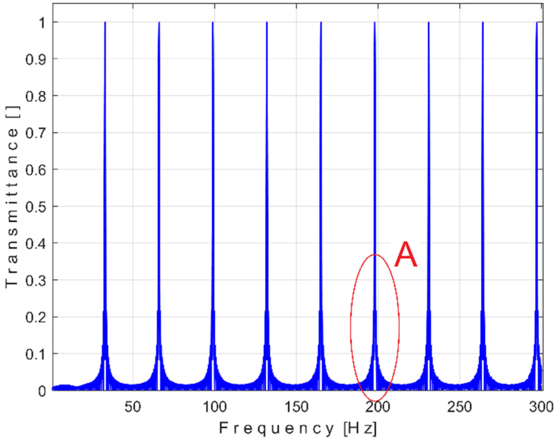
Figure 2.
A zooming-in in area A from Figure 1.
Figure 2.
A zooming-in in area A from Figure 1.
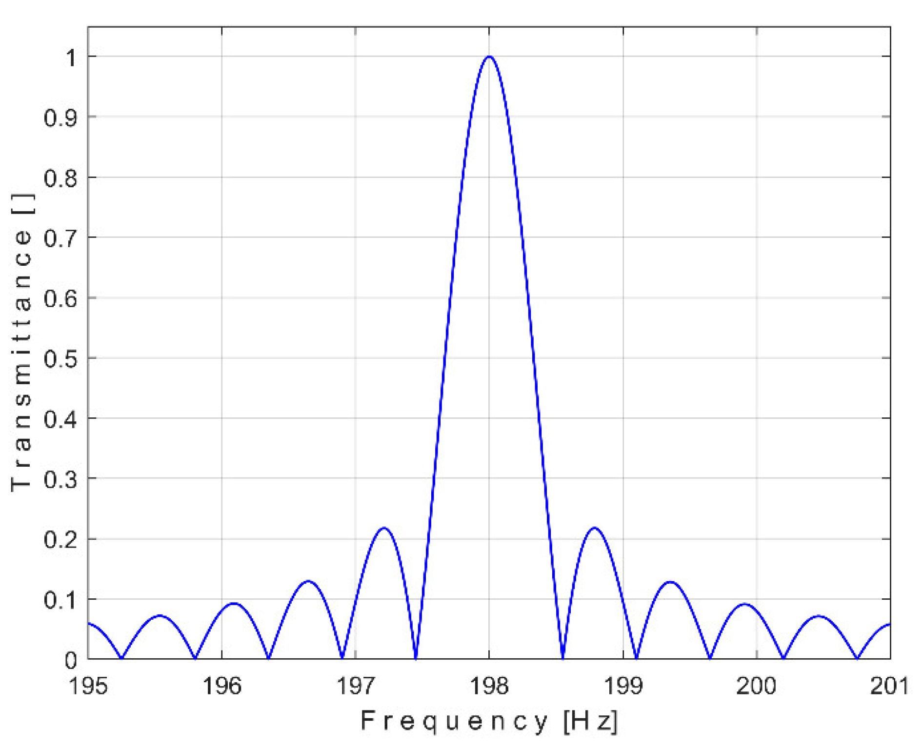
Figure 3.
The time-domain representation of the residuals s[k]-sT[k] over time k·Δt, with k=1÷n, T=1s, Δt=25,000.
Figure 3.
The time-domain representation of the residuals s[k]-sT[k] over time k·Δt, with k=1÷n, T=1s, Δt=25,000.

Figure 4.
The time-domain representations of the residuals s[k]-sT[k] over time k·Δt, with k=1÷n, T=1s. Curve 1 - Δt=1/25,000.5 (with
Figure 4.
The time-domain representations of the residuals s[k]-sT[k] over time k·Δt, with k=1÷n, T=1s. Curve 1 - Δt=1/25,000.5 (with
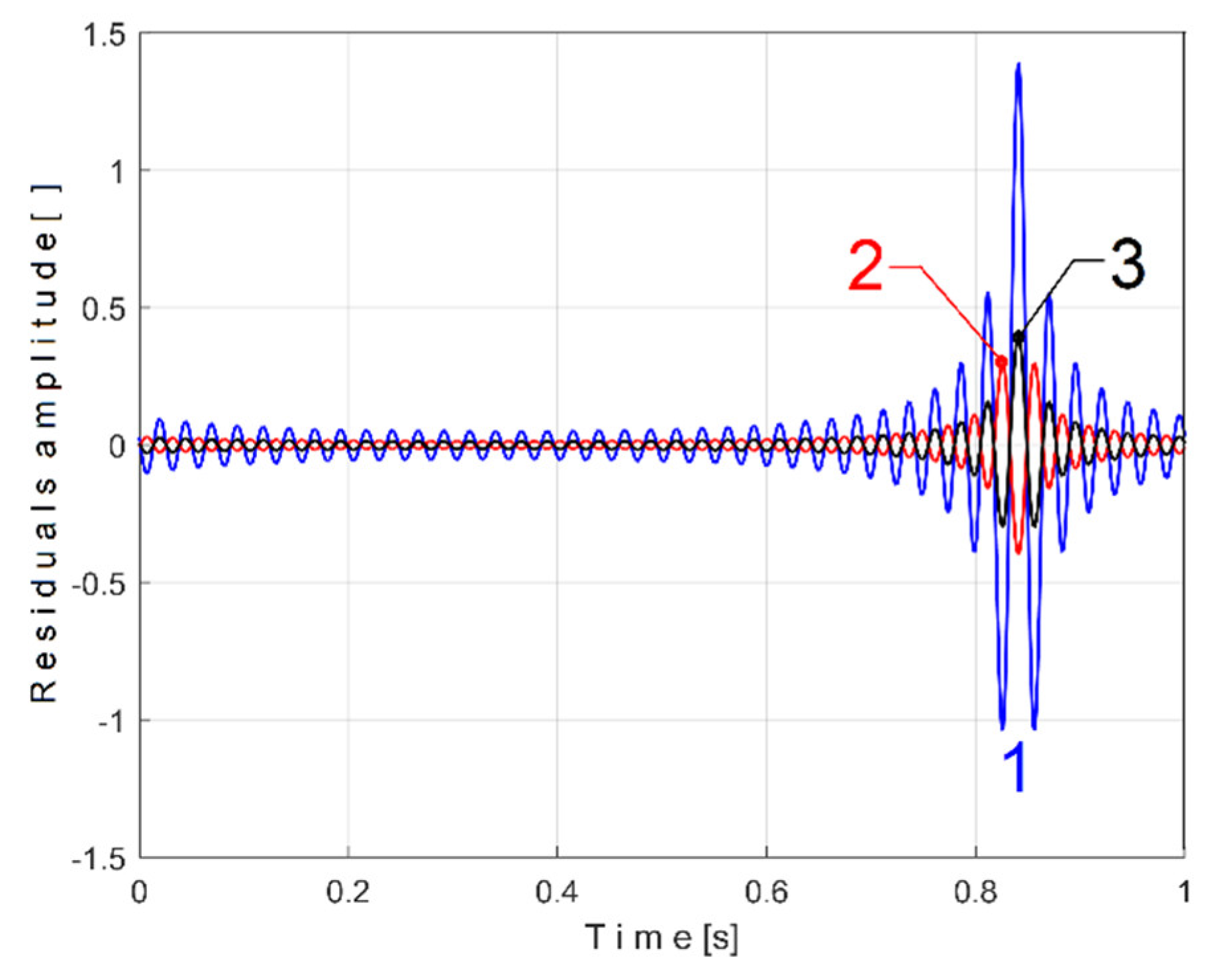
Figure 5.
A sequence of the random noise signal rn during a period T.
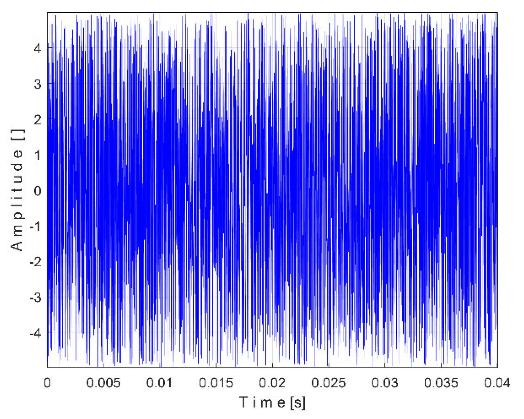
Figure 6.
A description of the periodical signal s from Eq. (5) during a period T=1/25 Hz.
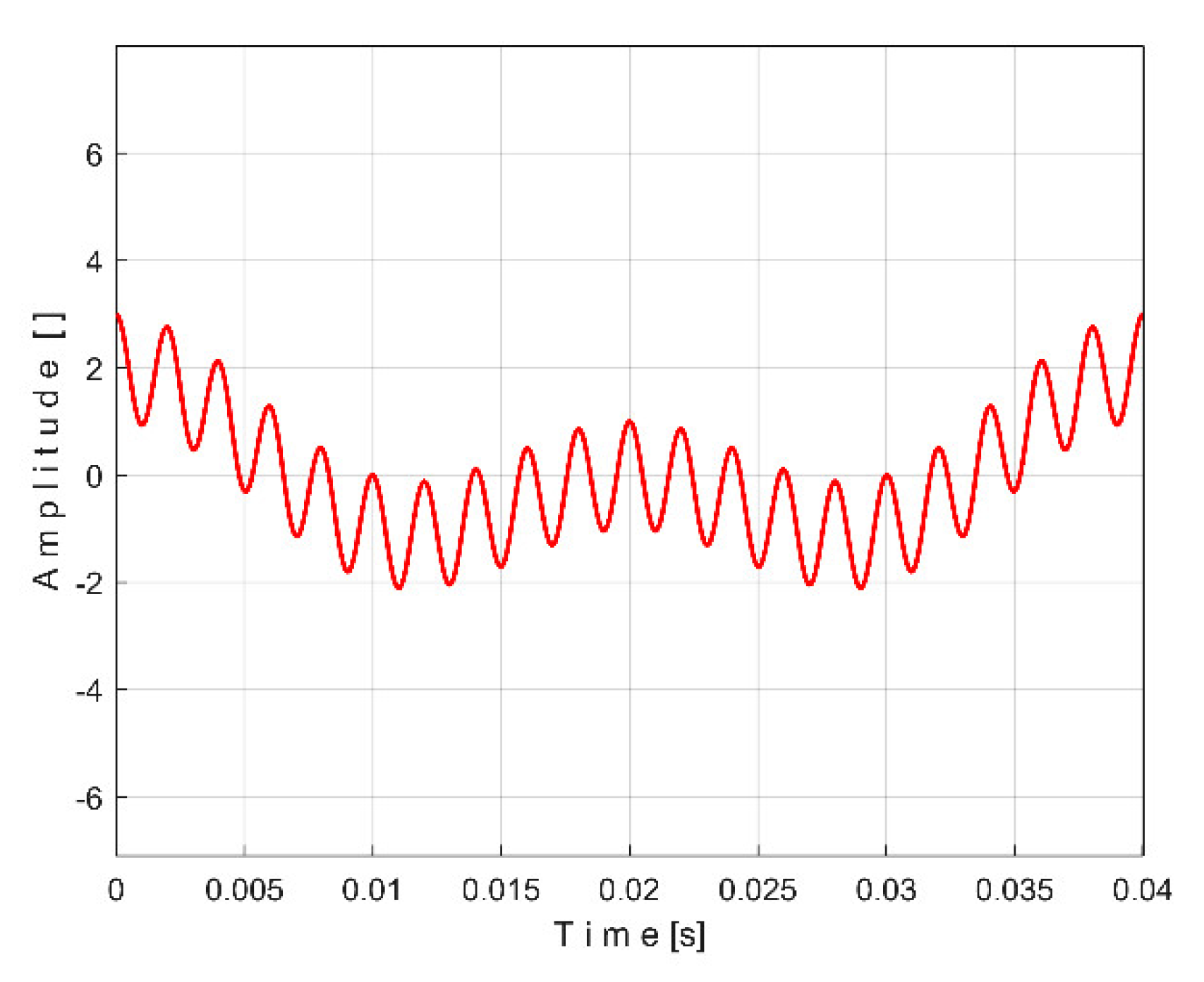
Figure 7.
A description of the mixed signals rn+s during a period T.
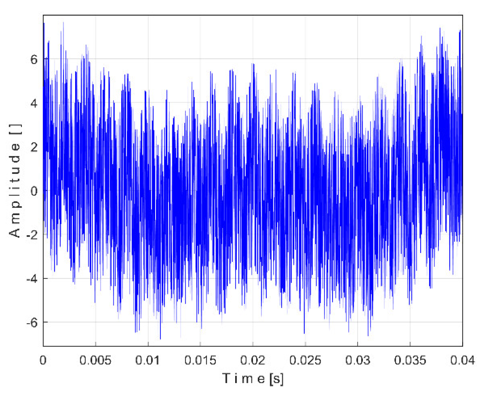
Figure 8.
1 – A period of signal s from Eq. (5); 2 – The sT pattern obtained by AMSSRTI applied on rn+s signal, with m=100 and T=1/25 s.
Figure 8.
1 – A period of signal s from Eq. (5); 2 – The sT pattern obtained by AMSSRTI applied on rn+s signal, with m=100 and T=1/25 s.
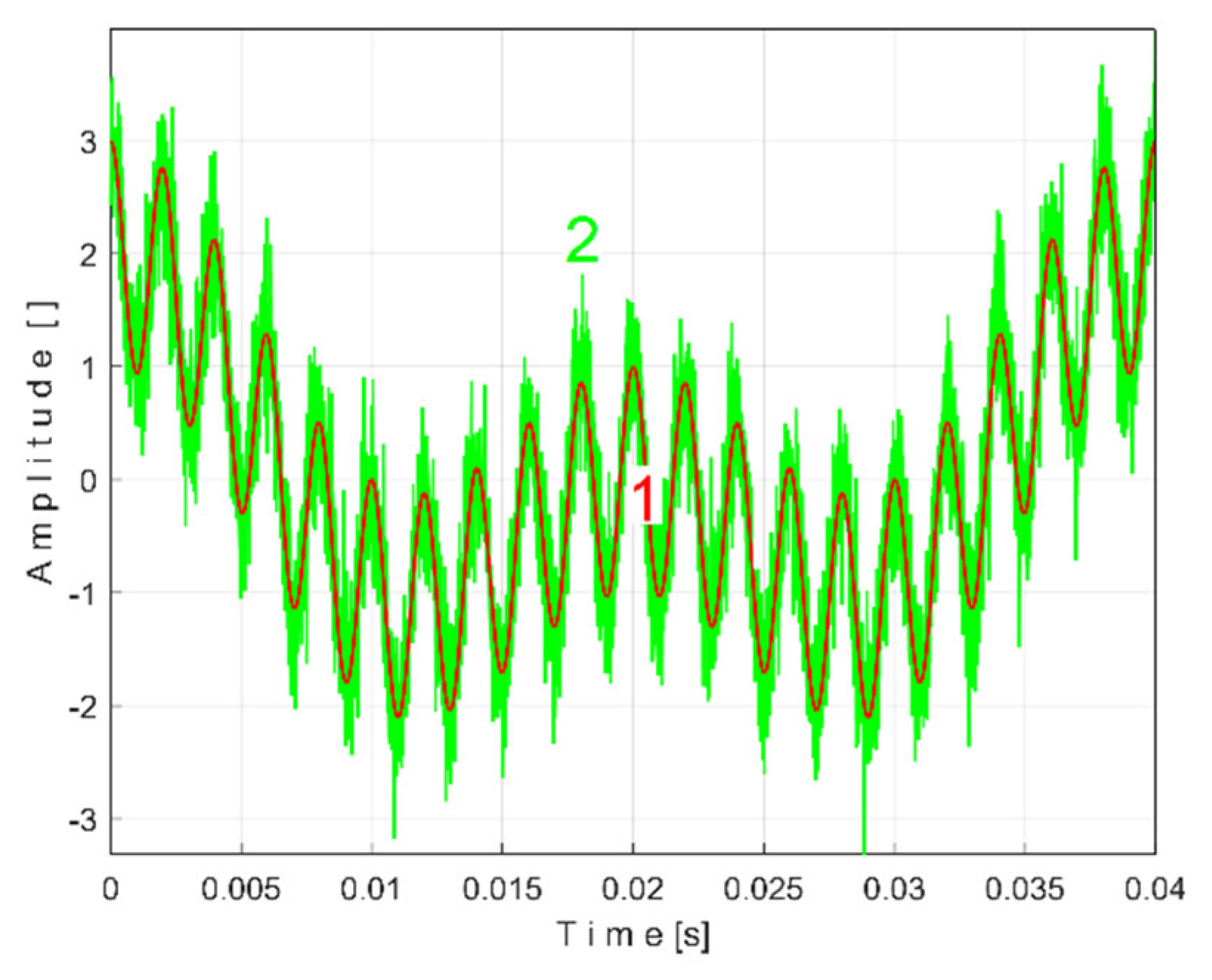
Figure 9.
1 – A period of signal s from Eq. (5); 2 – The sT pattern obtained by AMSSRTI with m=500 and T=1/25 s.
Figure 9.
1 – A period of signal s from Eq. (5); 2 – The sT pattern obtained by AMSSRTI with m=500 and T=1/25 s.
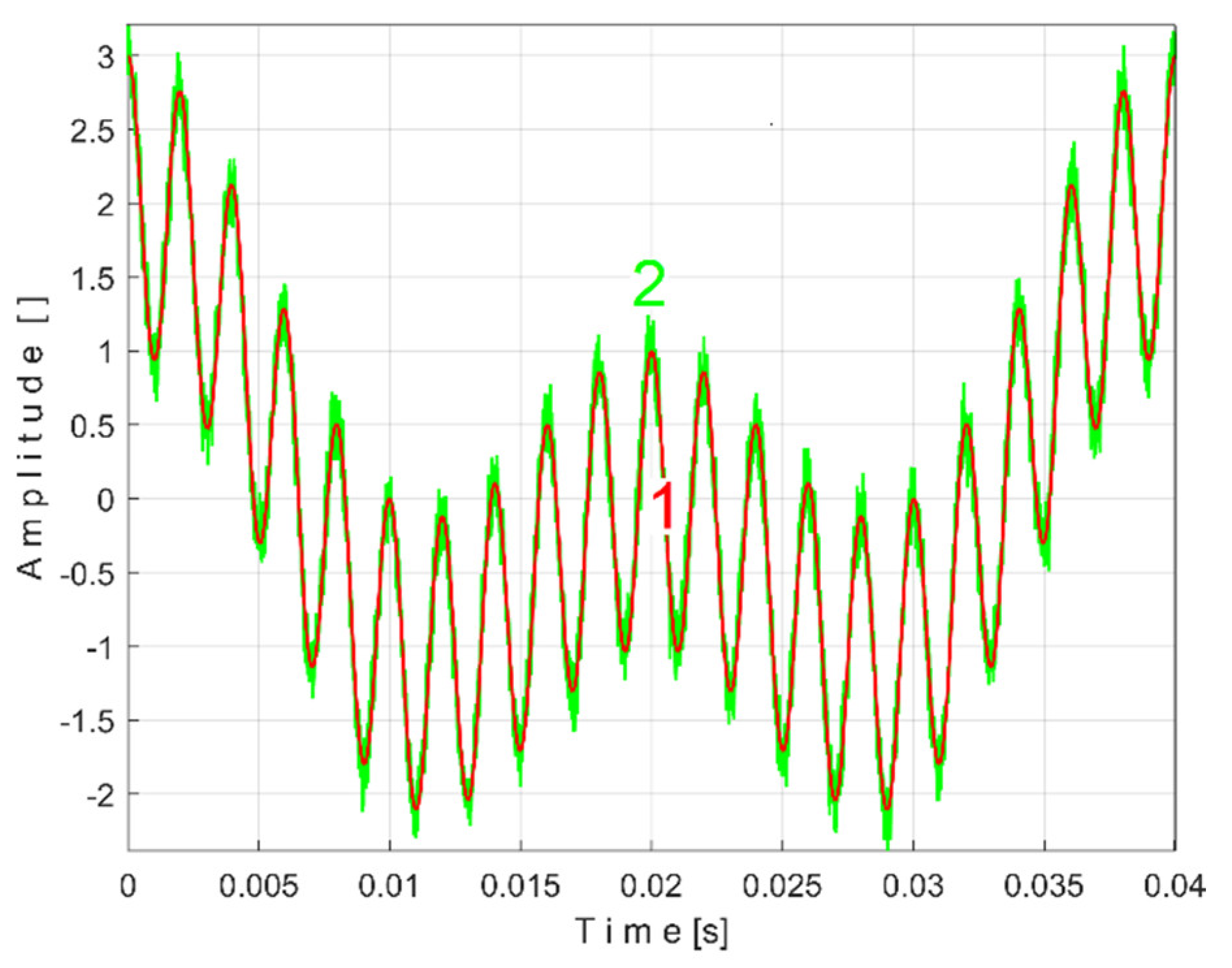
Figure 10.
1 – A description of the experimental setup [3].
Figure 10.
1 – A description of the experimental setup [3].
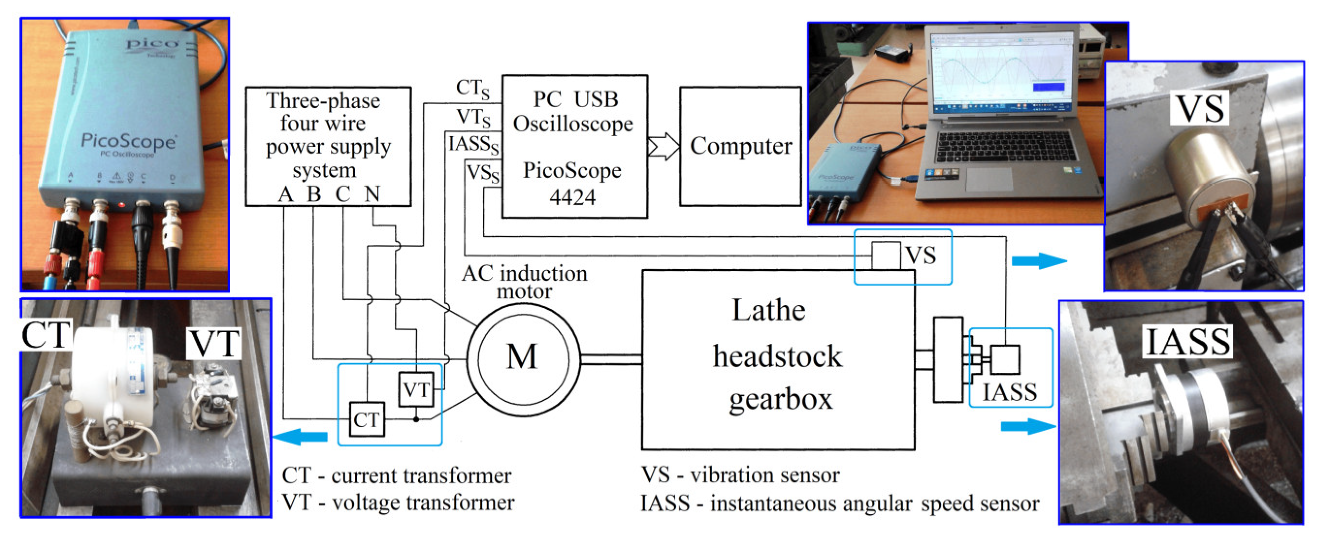
Figure 11.
The gearing diagram of the lathe headstock gearbox [3].
Figure 11.
The gearing diagram of the lathe headstock gearbox [3].
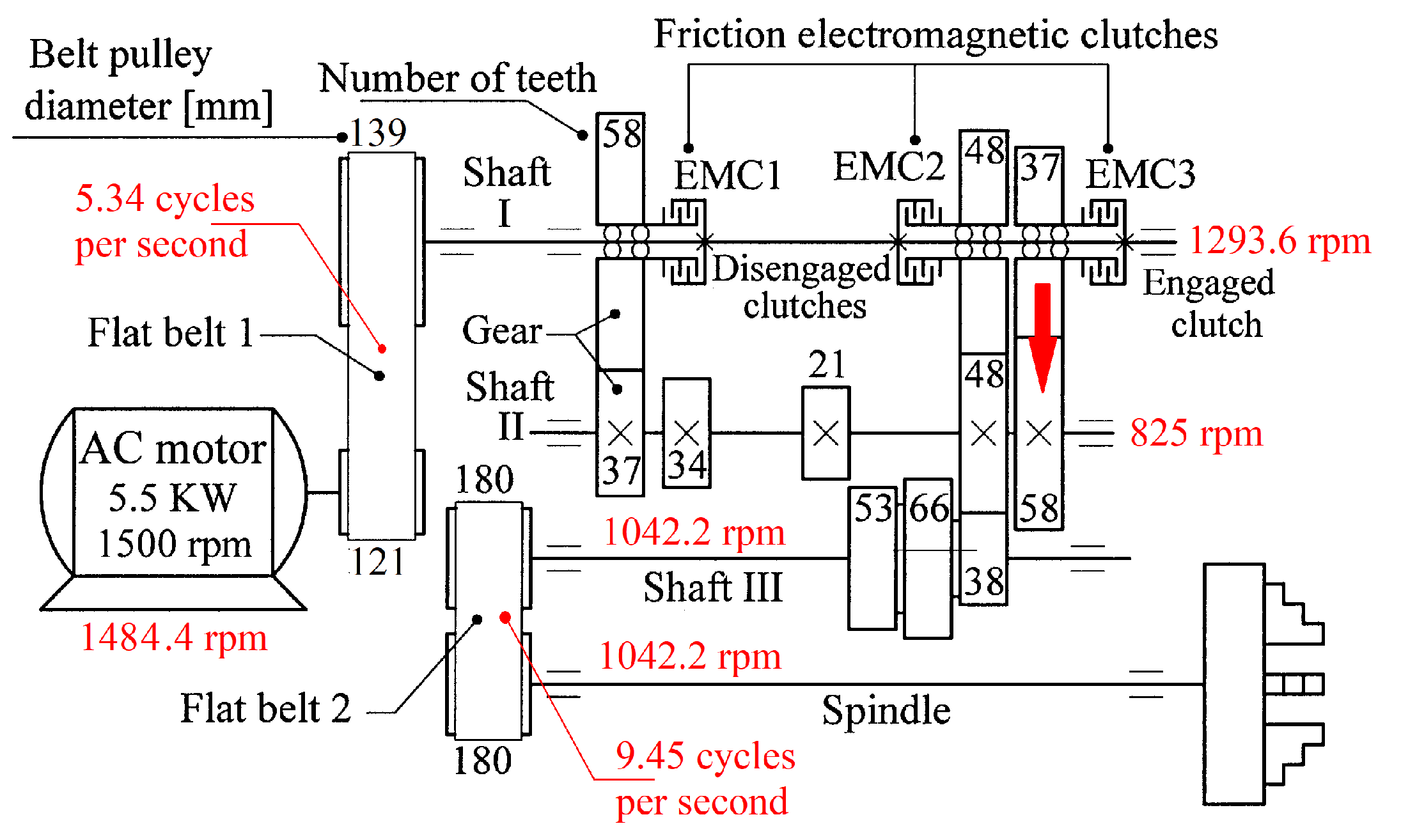
Figure 12.
The time-domain representations of: 1 - Pa; 2 –the very low frequency variable part of Pa.
Figure 12.
The time-domain representations of: 1 - Pa; 2 –the very low frequency variable part of Pa.
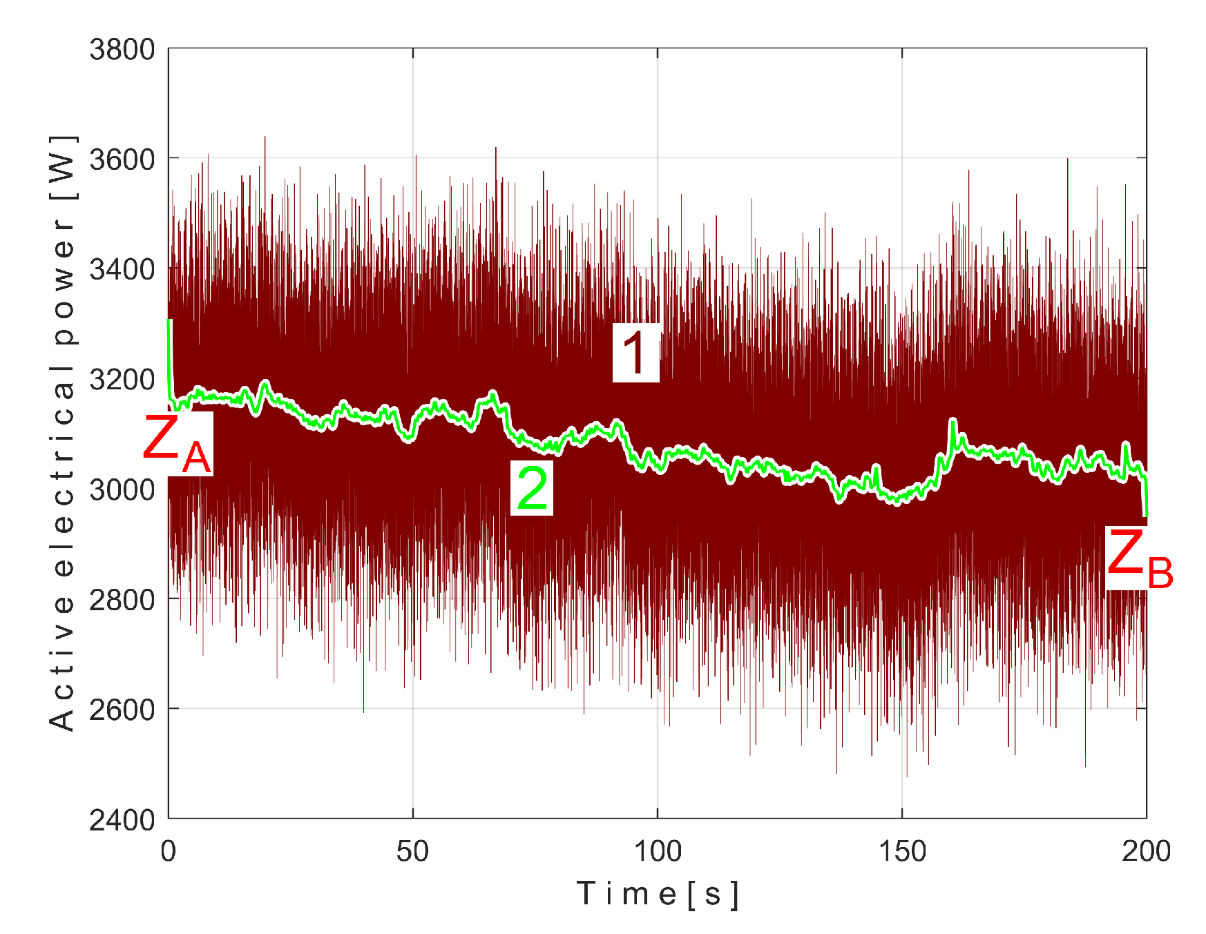
Figure 13.
The time-domain representation of Pav.
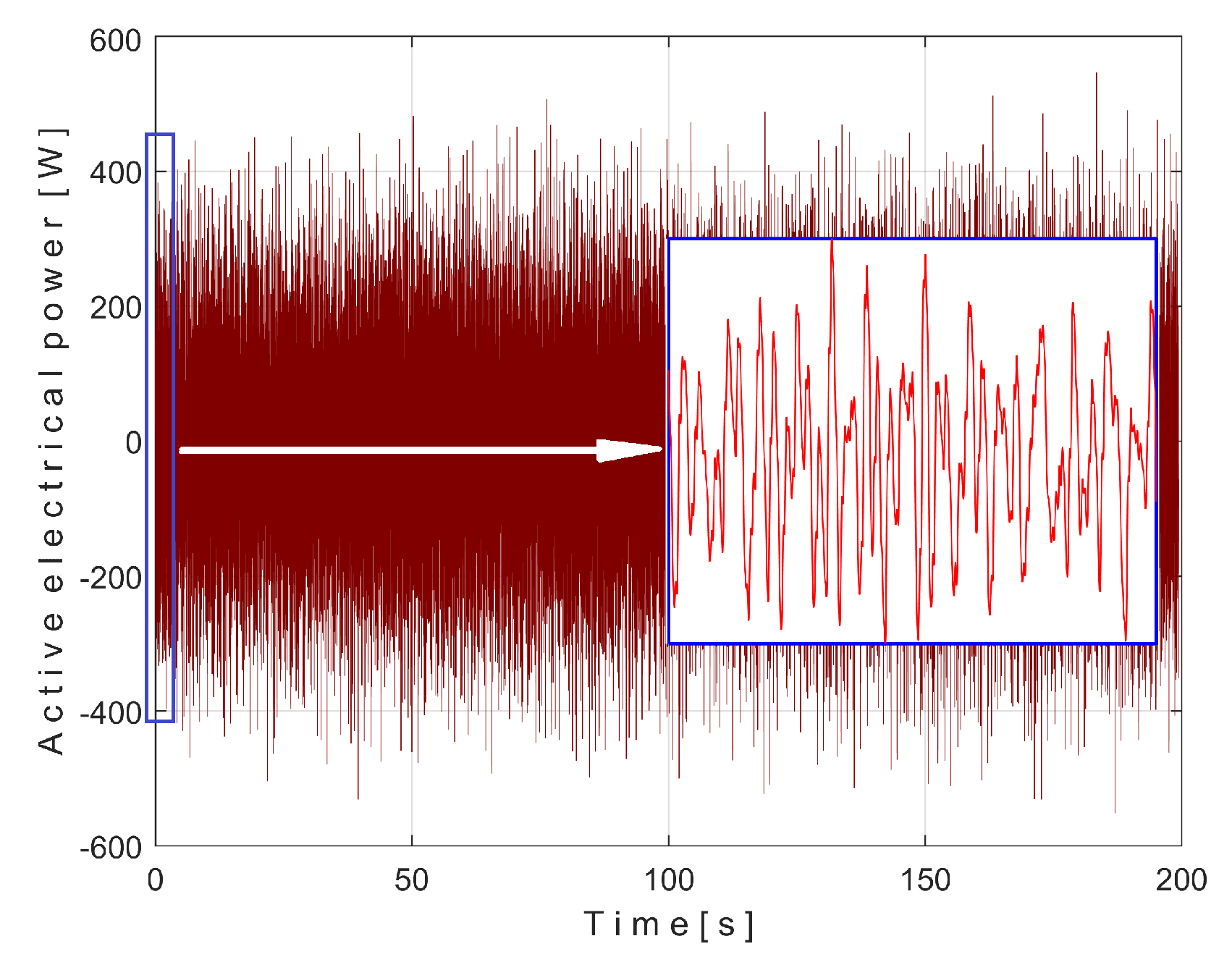
Figure 14.
The FFT spectrum of Pav with A ÷ E the fundamentals of PVSC generated by these MC: A – the flat belt 1; B – the flat belt 2; C – the shaft II; D - the shaft III and the main spindle; E – the shaft I.
Figure 14.
The FFT spectrum of Pav with A ÷ E the fundamentals of PVSC generated by these MC: A – the flat belt 1; B – the flat belt 2; C – the shaft II; D - the shaft III and the main spindle; E – the shaft I.
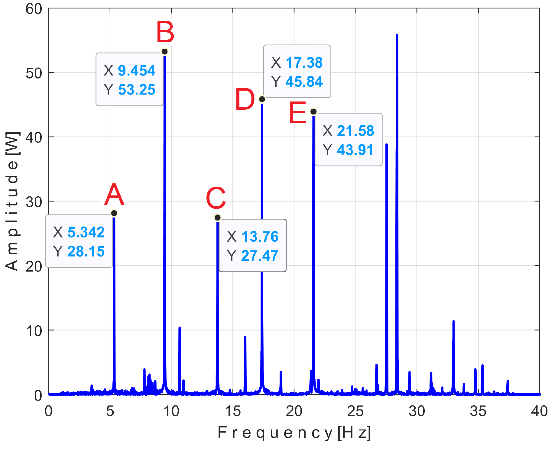
Figure 15.
The extended AMSSRTI patterns (m = 530) which describes the behaviour of first flat belt in signal sP: 1- sPTAe5a (fPAa = 5.33748 Hz); 2- sPTAe5b (fPAb = 5.34162 Hz).
Figure 15.
The extended AMSSRTI patterns (m = 530) which describes the behaviour of first flat belt in signal sP: 1- sPTAe5a (fPAa = 5.33748 Hz); 2- sPTAe5b (fPAb = 5.34162 Hz).
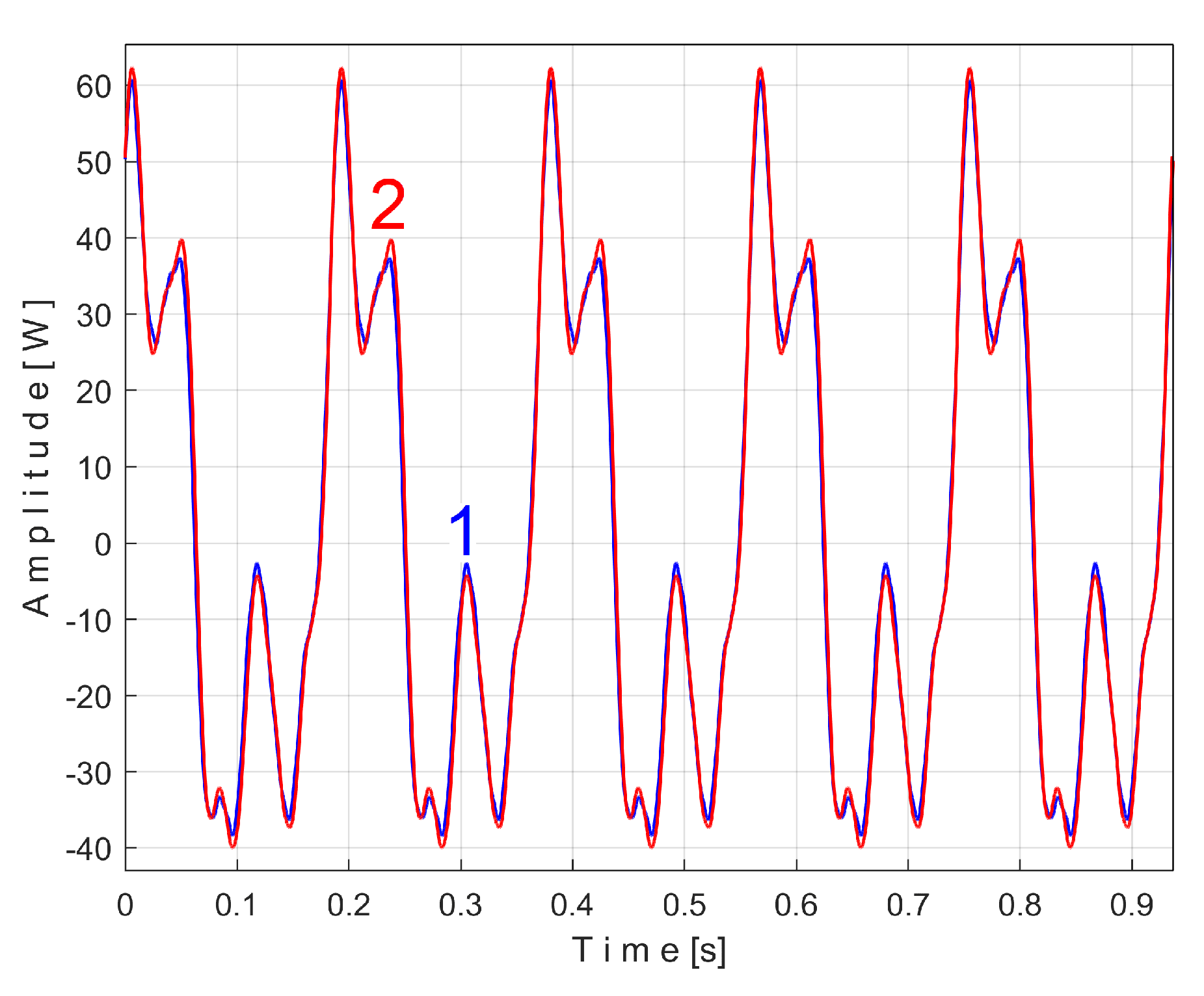
Figure 16.
1 - The extended pattern sPTAe5b (m = 530, fPAb = 5.3414 Hz); 2 – The analytical description of this pattern (with eight sinusoidal components, Table 2); 3 – The residual (the difference between curves 1 and 2);.
Figure 16.
1 - The extended pattern sPTAe5b (m = 530, fPAb = 5.3414 Hz); 2 – The analytical description of this pattern (with eight sinusoidal components, Table 2); 3 – The residual (the difference between curves 1 and 2);.
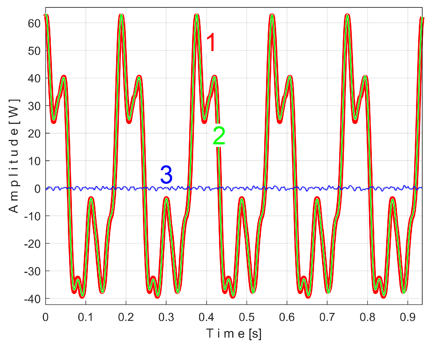
Figure 17.
The FFT spectra of: 1 - the sequence sP50; 2 - the signal sP1r50. .
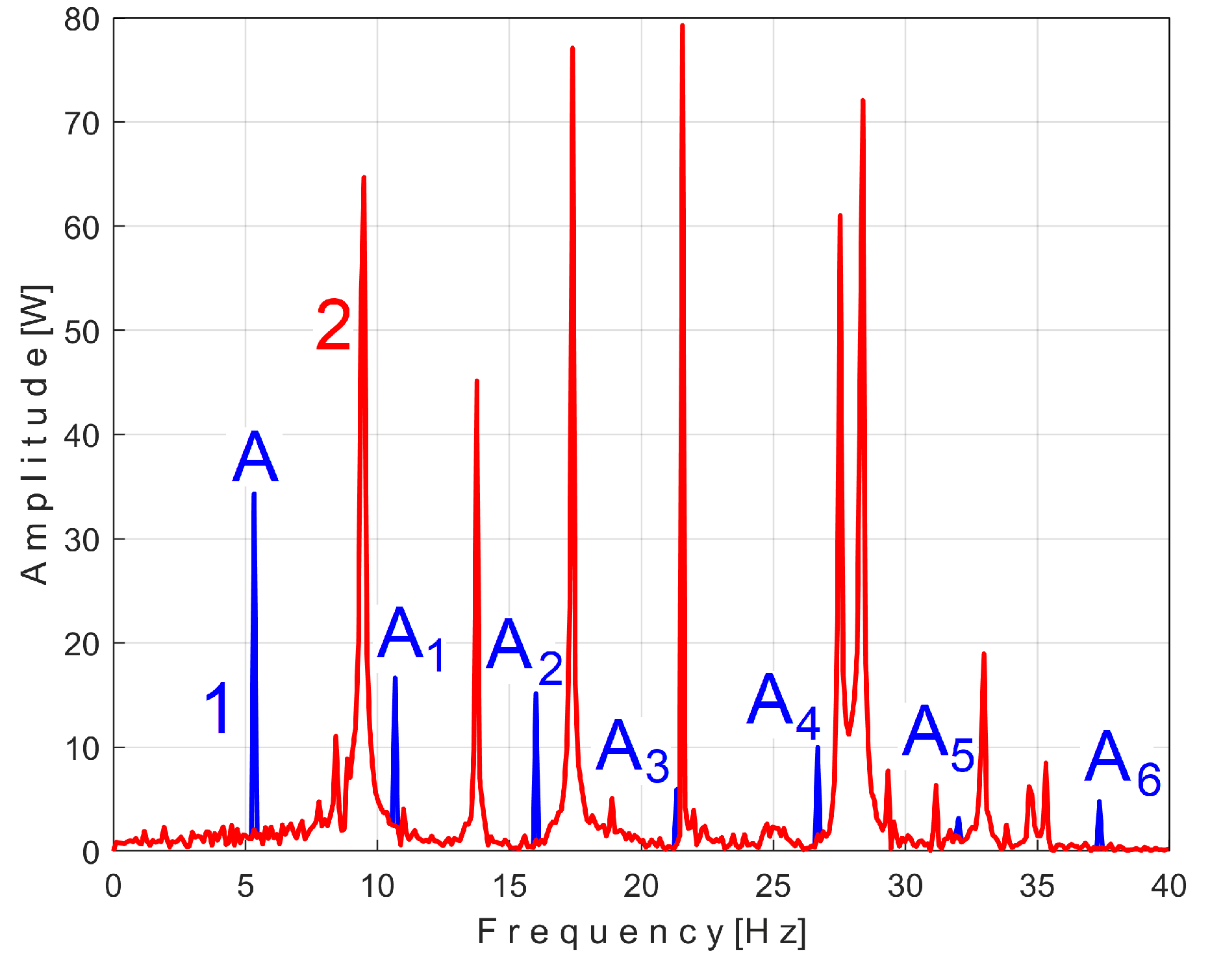
Figure 18.
The extended AMSSRTI patterns (m = 935) describing the behaviour of second flat belt in signal sP: 1- sPTBe5a (fPBa = 9.45223 Hz); 2 – sPTBe5b (fPBb = 9.45981 Hz).
Figure 18.
The extended AMSSRTI patterns (m = 935) describing the behaviour of second flat belt in signal sP: 1- sPTBe5a (fPBa = 9.45223 Hz); 2 – sPTBe5b (fPBb = 9.45981 Hz).
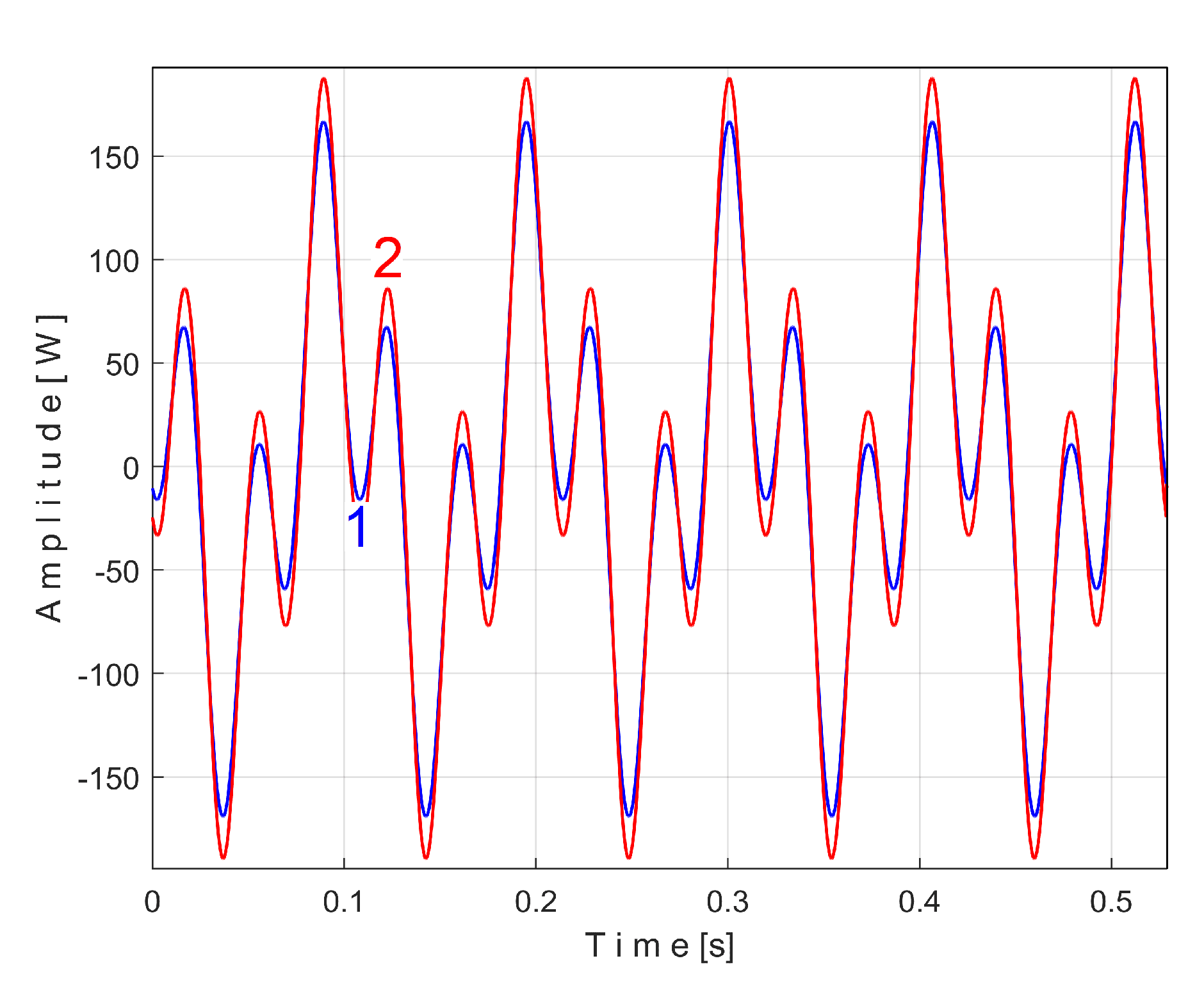
Figure 19.
The results of removing of the extended patterns sPTAe50 and sPTBe89* from sP50 in FFT spectrum. 1 – The FFT spectrum of the sequence sP50 (already depicted in Figure 17); 2 – The overlapped FFT spectrum of sequence sP1r50 (already depicted in Figure 17); 3 – The overlapped FFT spectrum of sequence sP2r50.
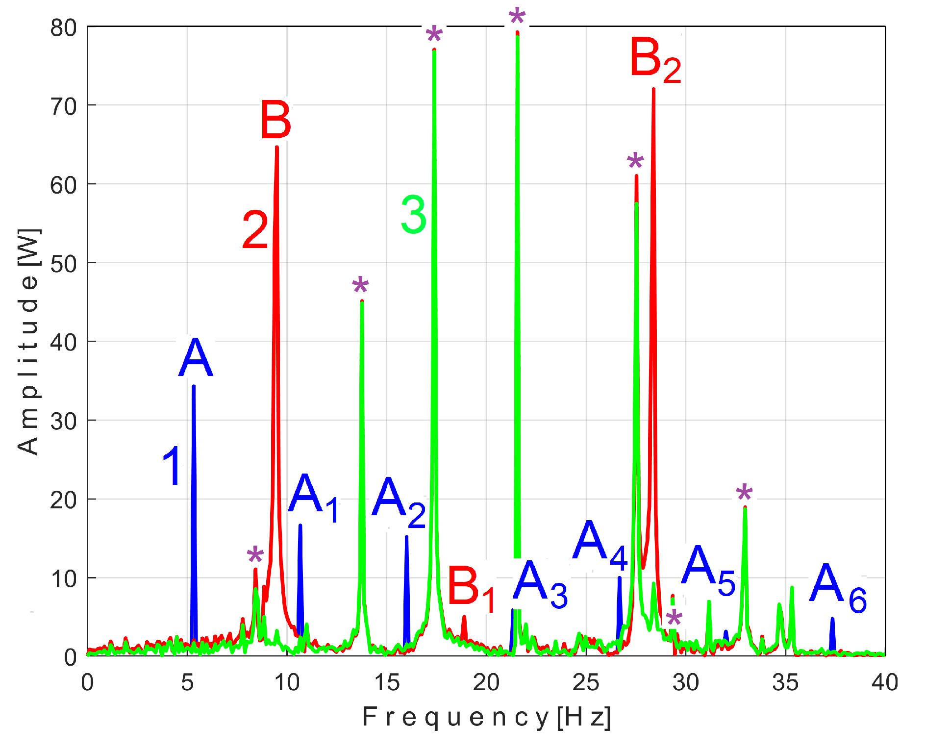
Figure 20.
The extended AMSSRTI patterns (m = 1350) describing the behaviour of the shaft II in signal sP: 1 - sPTCe5a (fPCa = 13.75435 Hz); 2 –sPTCe5b (fPCb = 13.759 Hz).
Figure 20.
The extended AMSSRTI patterns (m = 1350) describing the behaviour of the shaft II in signal sP: 1 - sPTCe5a (fPCa = 13.75435 Hz); 2 –sPTCe5b (fPCb = 13.759 Hz).
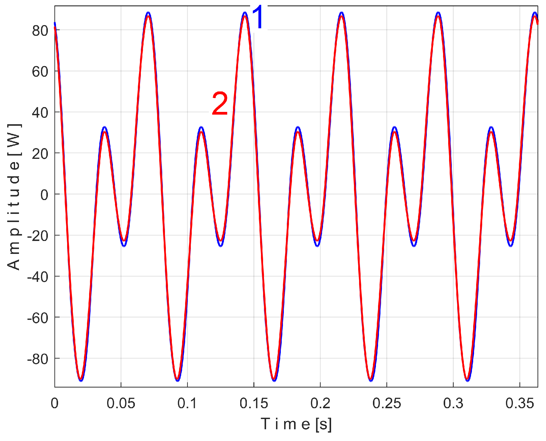
Figure 21.
The extended AMSSRTI patterns (m = 1720) describing the behaviour of the shaft III and spindle in signal sP: 1 - sPTDe5a (fPDa = 17.37406 Hz); 2 – sPTDe5b (fPDb = 17.38745 Hz).
Figure 21.
The extended AMSSRTI patterns (m = 1720) describing the behaviour of the shaft III and spindle in signal sP: 1 - sPTDe5a (fPDa = 17.37406 Hz); 2 – sPTDe5b (fPDb = 17.38745 Hz).
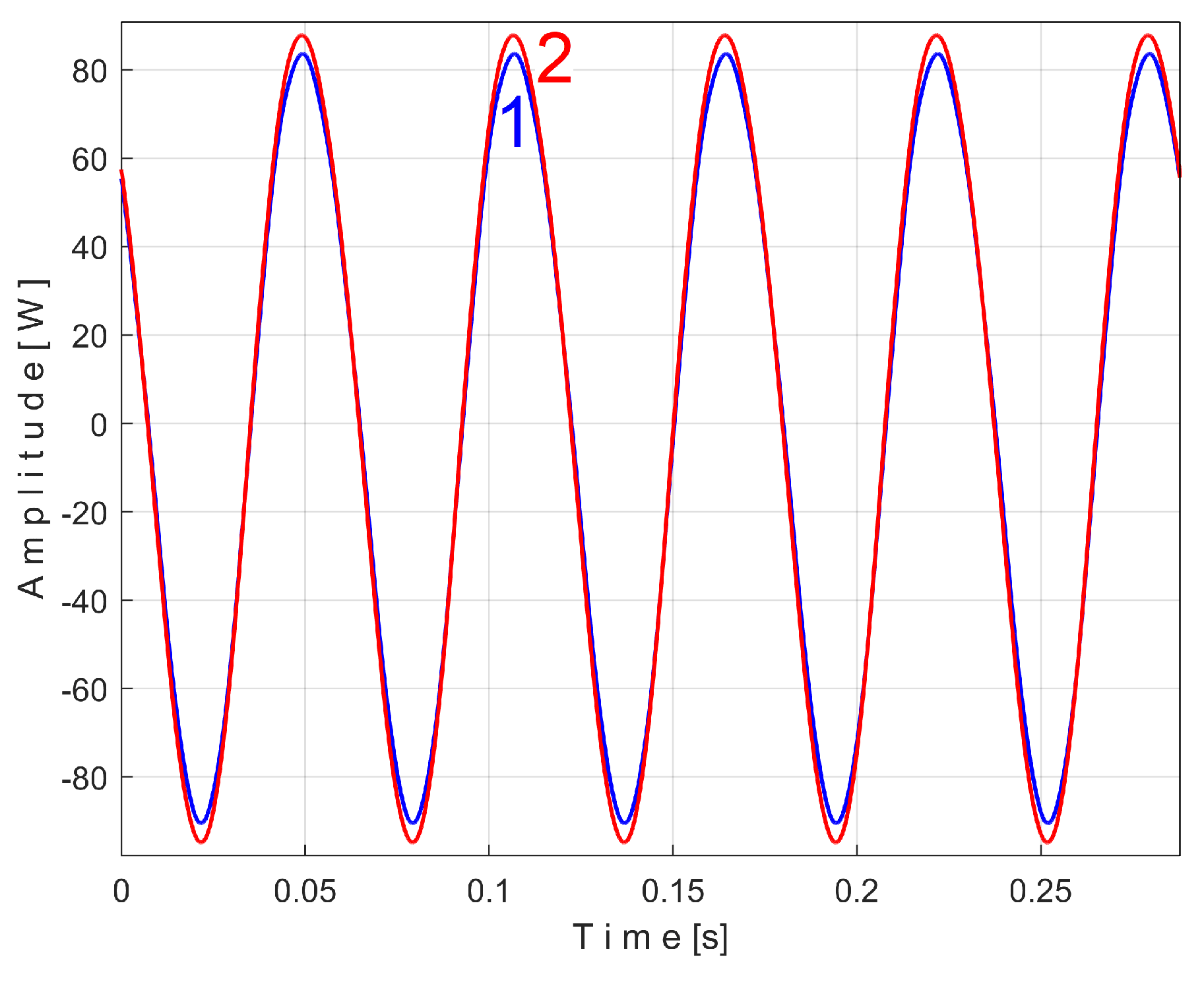
Figure 22.
The extended AMSSRTI patterns (m = 2130) describing the behaviour of the shaft II in signal sP: 1 - sPTEe5a (fPEa = 21.5606 Hz); 2 –sPTDe5b (fPEb = 21.5781 Hz).
Figure 22.
The extended AMSSRTI patterns (m = 2130) describing the behaviour of the shaft II in signal sP: 1 - sPTEe5a (fPEa = 21.5606 Hz); 2 –sPTDe5b (fPEb = 21.5781 Hz).
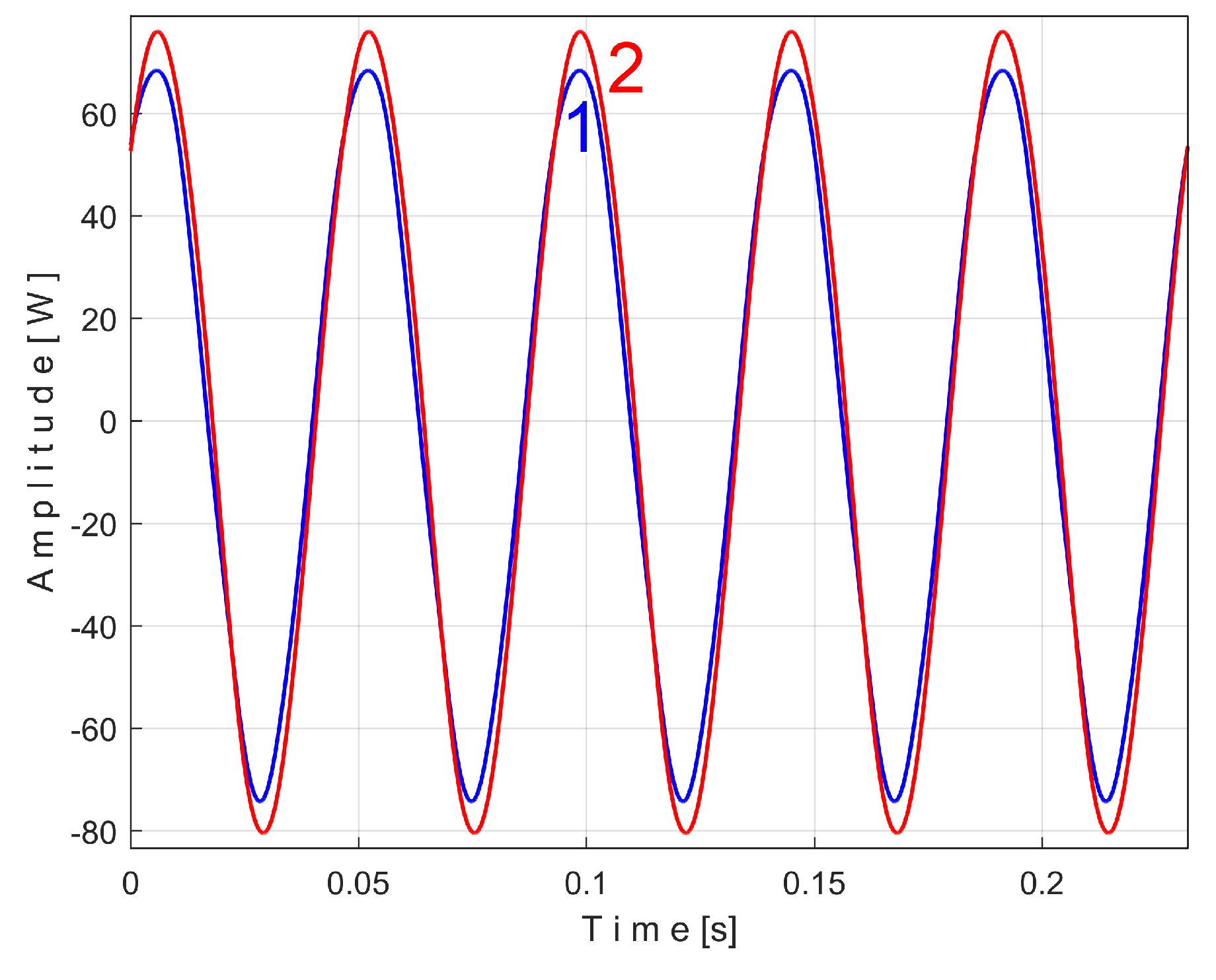
Figure 23.
The time-domain representation of the signal Vs.
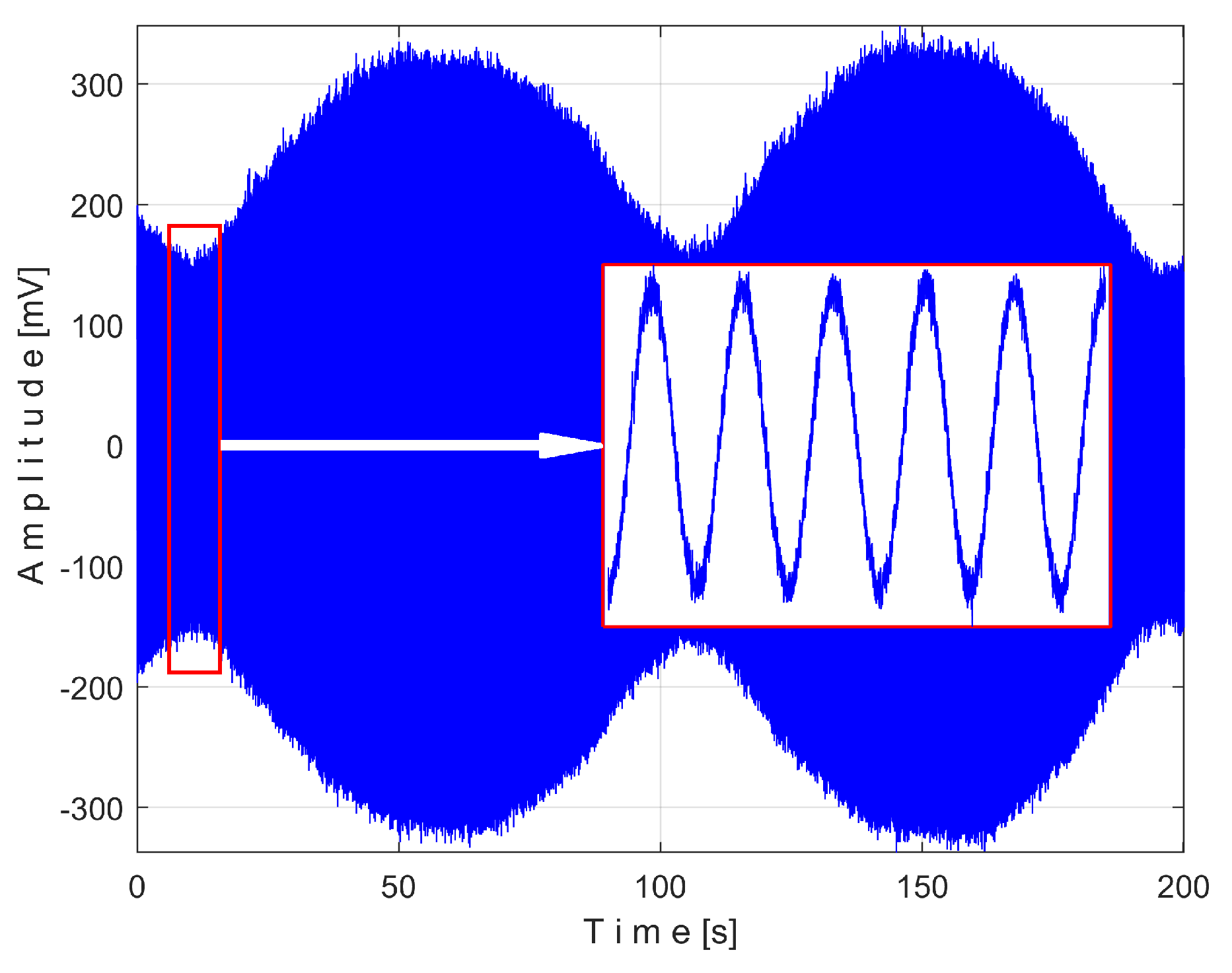
Figure 24.
The FFT spectrum of Vs with A ÷ E the fundamentals of PVSC generated by these MC: A – the flat belt 1; B – the flat belt 2; C – the shaft II; D - the shaft III and the spindle; E – the shaft I.
Figure 24.
The FFT spectrum of Vs with A ÷ E the fundamentals of PVSC generated by these MC: A – the flat belt 1; B – the flat belt 2; C – the shaft II; D - the shaft III and the spindle; E – the shaft I.
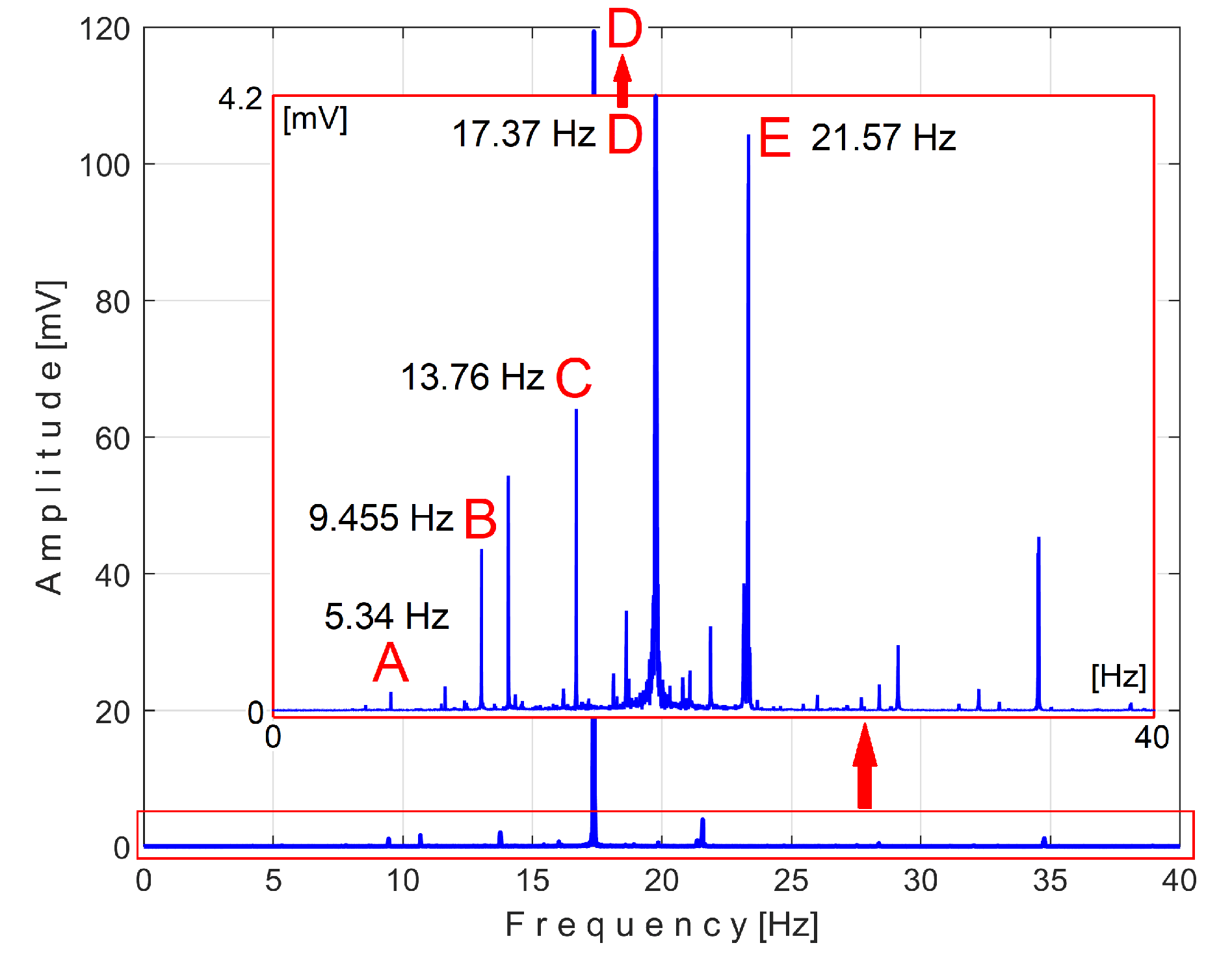
Figure 25.
The low-pass filtered extended AMSSRTI patterns (m = 533) describing the behaviour of the flat belt 1 in signal sV: 1 - sVTAe5a, fVAa = 5.33736 Hz; 2 - sVTAe5b, fVAb = 5.34151 Hz.
Figure 25.
The low-pass filtered extended AMSSRTI patterns (m = 533) describing the behaviour of the flat belt 1 in signal sV: 1 - sVTAe5a, fVAa = 5.33736 Hz; 2 - sVTAe5b, fVAb = 5.34151 Hz.
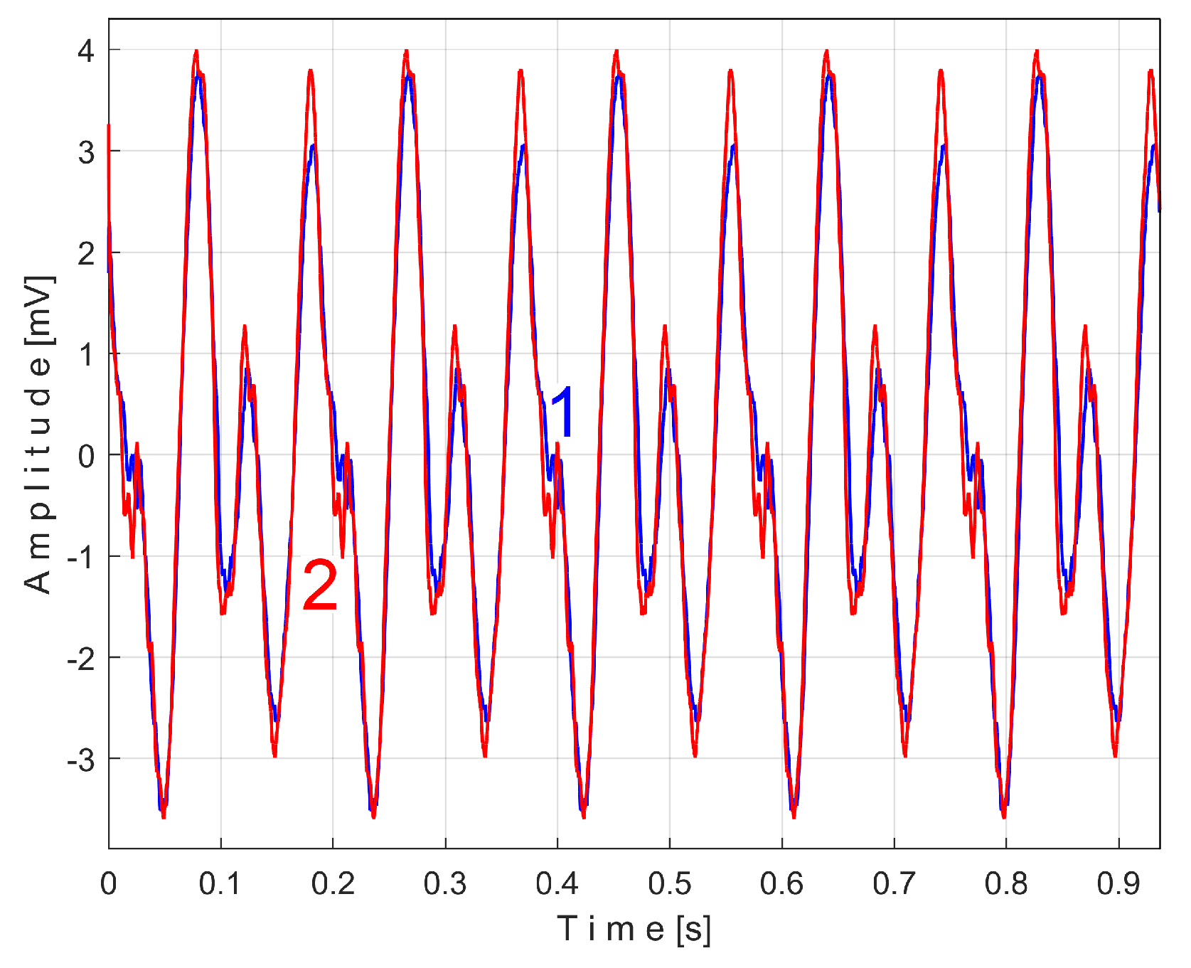
Figure 26.
The unfiltered extended patterns from Figure 25.
Figure 26.
The unfiltered extended patterns from Figure 25.
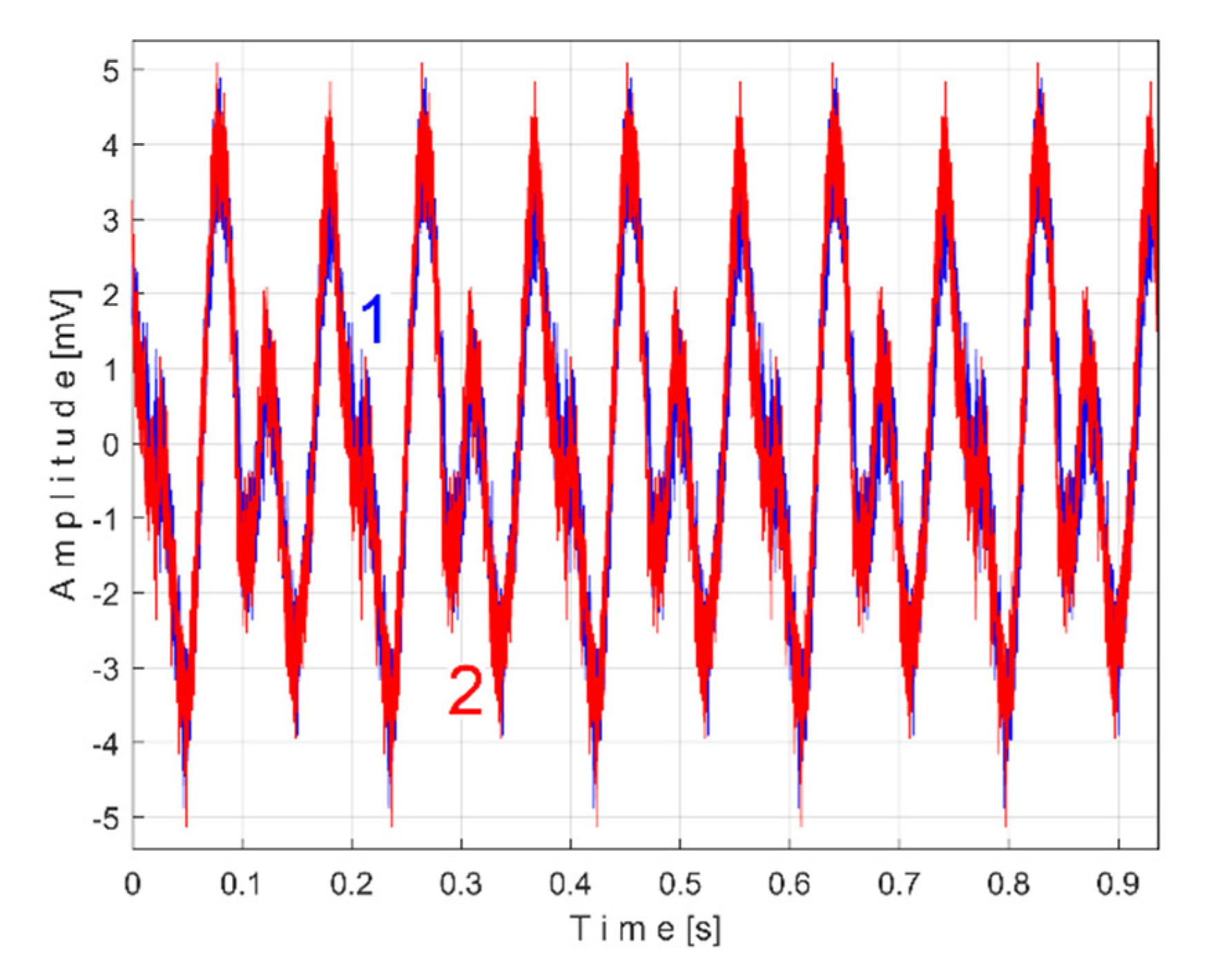
Figure 27.
The FFT spectrum of the extended unfiltered pattern sVTAe50b.
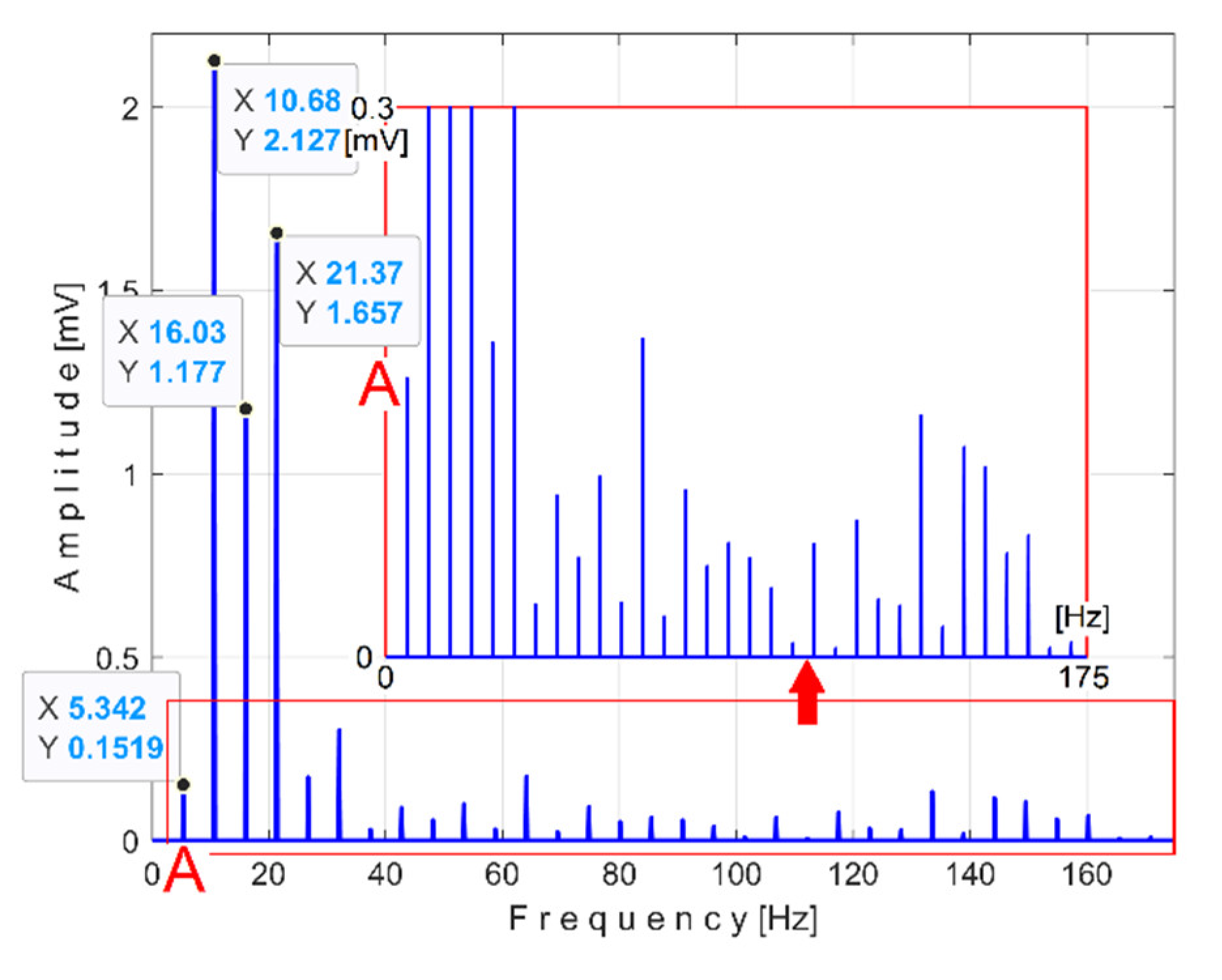
Figure 28.
The unfiltered extended AMSSRTI patterns (m = 935) describing the behaviour of the flat belt 2 in signal sV: 1 - sVTBe5a, fVBa = 9.4525 Hz; 2 - sVTBe5b, fVBb = 9.4596 Hz.
Figure 28.
The unfiltered extended AMSSRTI patterns (m = 935) describing the behaviour of the flat belt 2 in signal sV: 1 - sVTBe5a, fVBa = 9.4525 Hz; 2 - sVTBe5b, fVBb = 9.4596 Hz.
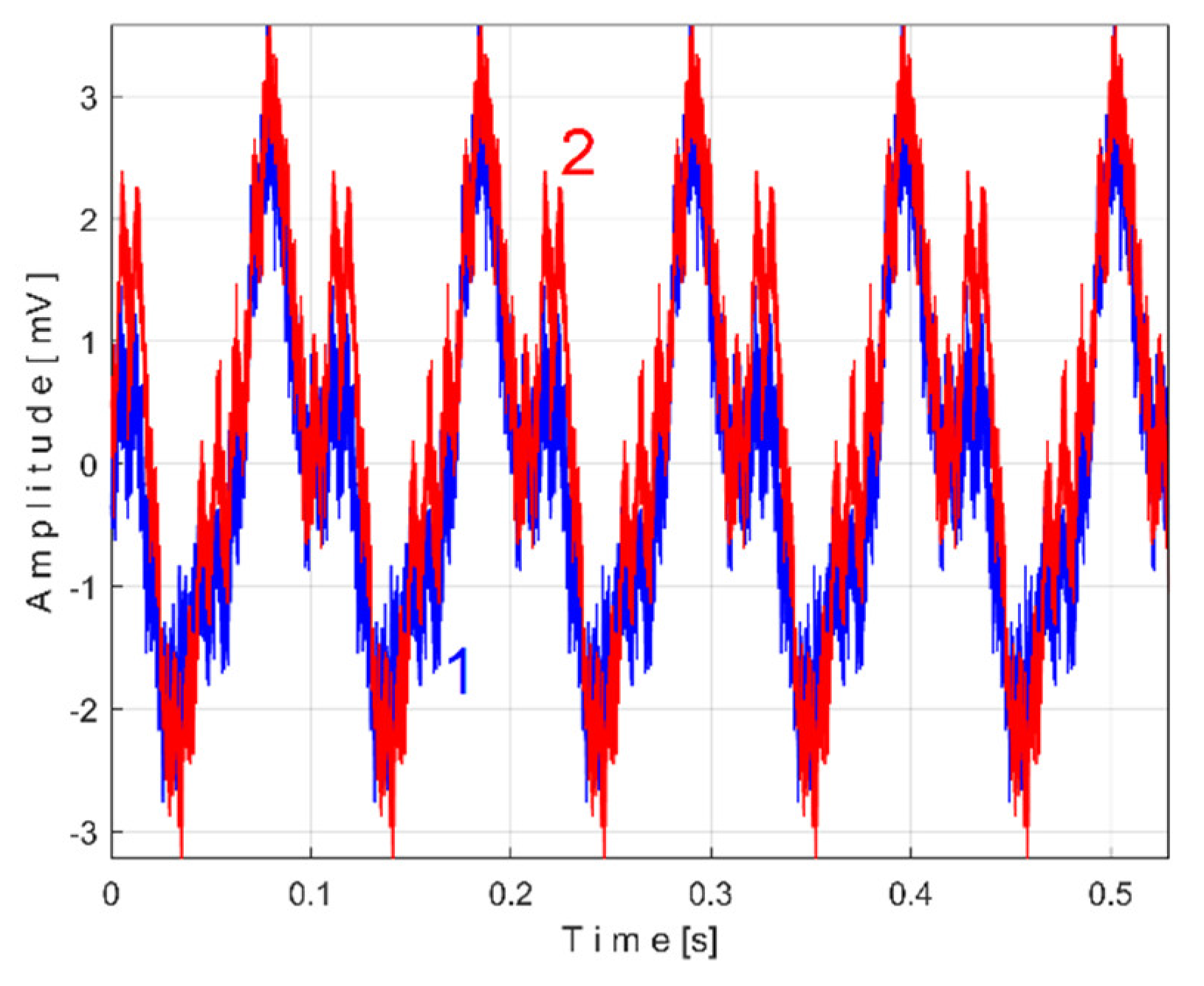
Figure 29.
The low-pass filtered extended patterns from Figure 28 (using a moving average filter with 30 samples in the average). .
Figure 29.
The low-pass filtered extended patterns from Figure 28 (using a moving average filter with 30 samples in the average). .
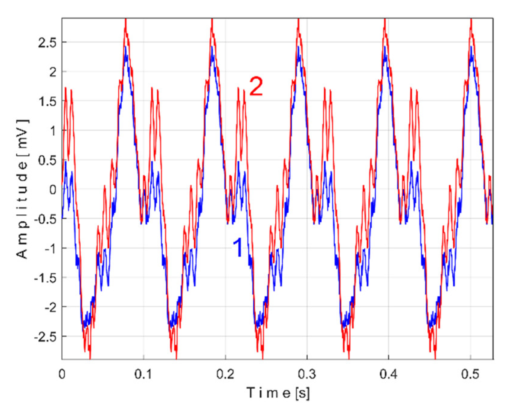
Figure 30.
The unfiltered extended AMSSRTI patterns (m = 1365) describing the behaviour of shaft II in signal sV: 1 - sVTCe5a, fVCa = 13.75399 Hz; 2 - sVTCe5b, fVCb = 13.76565 Hz.
Figure 30.
The unfiltered extended AMSSRTI patterns (m = 1365) describing the behaviour of shaft II in signal sV: 1 - sVTCe5a, fVCa = 13.75399 Hz; 2 - sVTCe5b, fVCb = 13.76565 Hz.
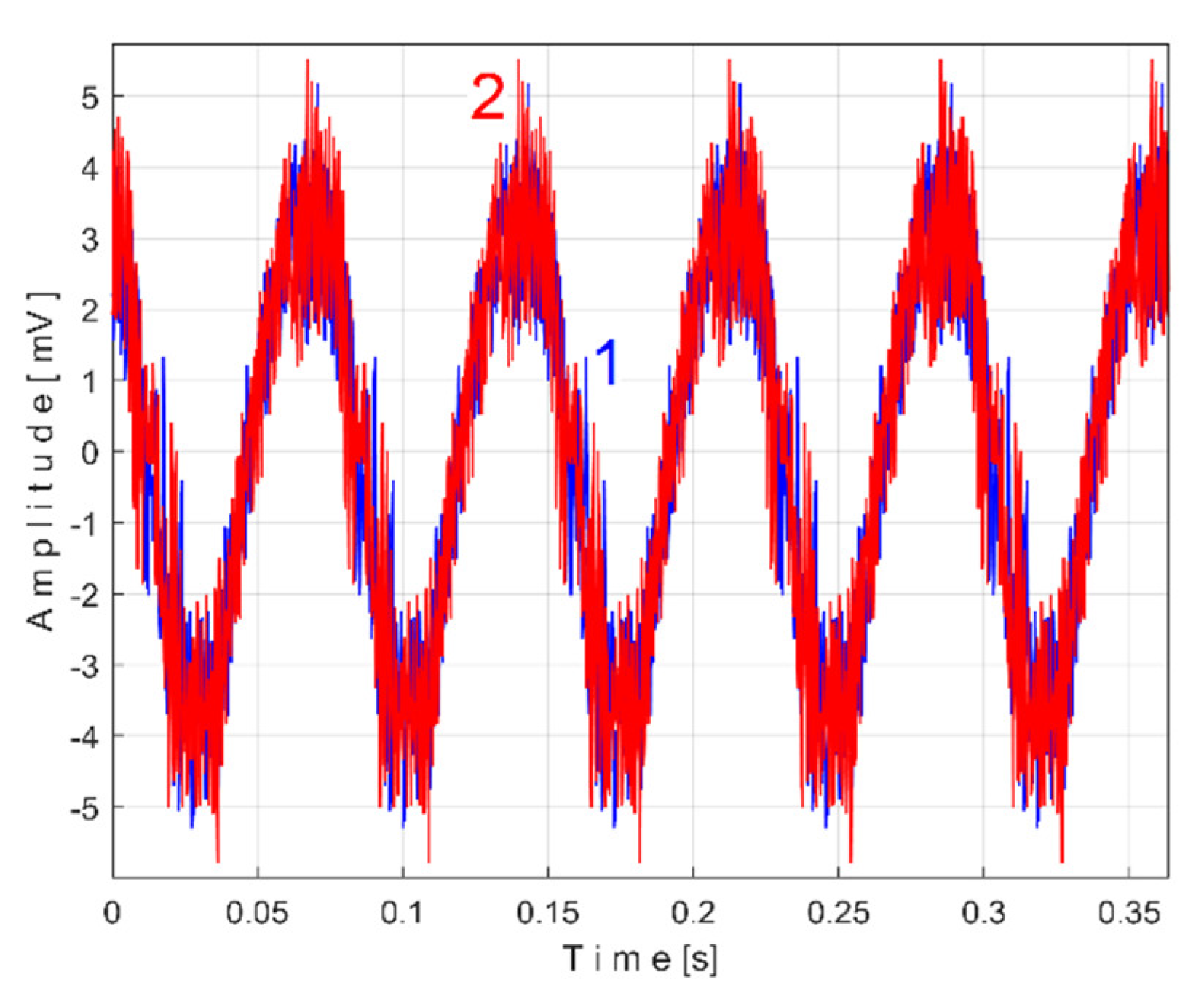
Figure 31.
The low-pass filtered extended patterns from Figure 30 (using a double moving average filter with 37 and 50 samples in the average). .
Figure 31.
The low-pass filtered extended patterns from Figure 30 (using a double moving average filter with 37 and 50 samples in the average). .
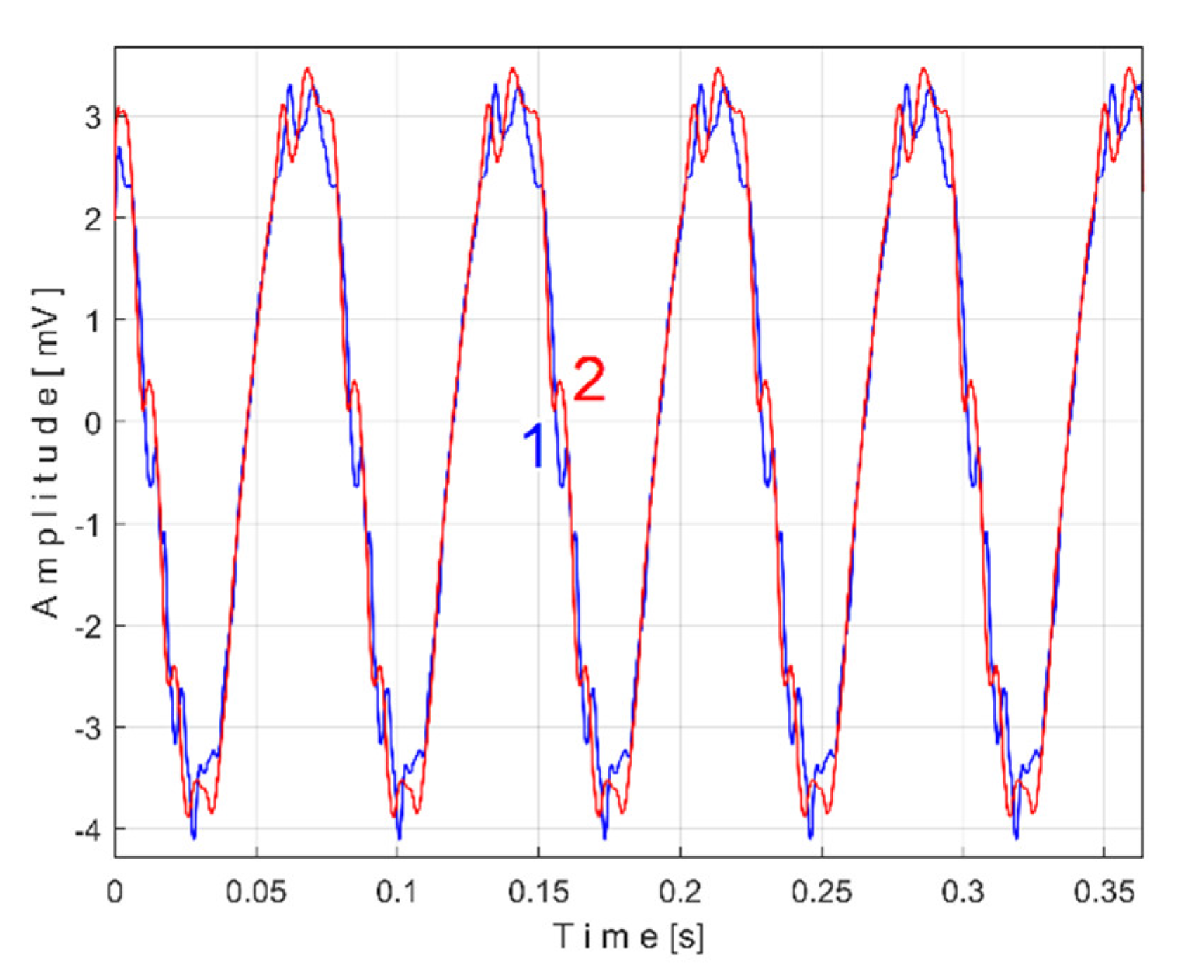
Figure 32.
2 – The unfiltered pattern sVTCe5b; 3 – An approximation of this pattern based on Eq. (7) as sVTCe5b2c.
Figure 32.
2 – The unfiltered pattern sVTCe5b; 3 – An approximation of this pattern based on Eq. (7) as sVTCe5b2c.
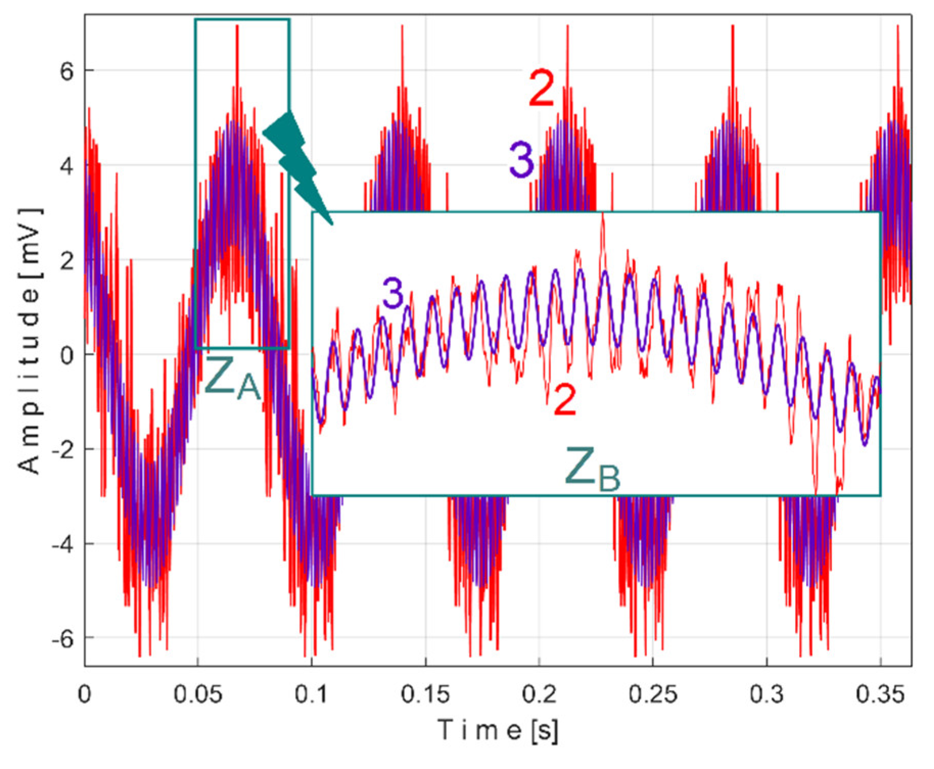
Figure 33.
The extended AMSSRTI patterns (m = 3250) describing the behavior of component TVC48 in signal sV: 1 - sVTC48e5a, fVC48a = 660.045986 Hz; 2 - sVTC48e5b, fVC48b = 660.53362 Hz.
Figure 33.
The extended AMSSRTI patterns (m = 3250) describing the behavior of component TVC48 in signal sV: 1 - sVTC48e5a, fVC48a = 660.045986 Hz; 2 - sVTC48e5b, fVC48b = 660.53362 Hz.
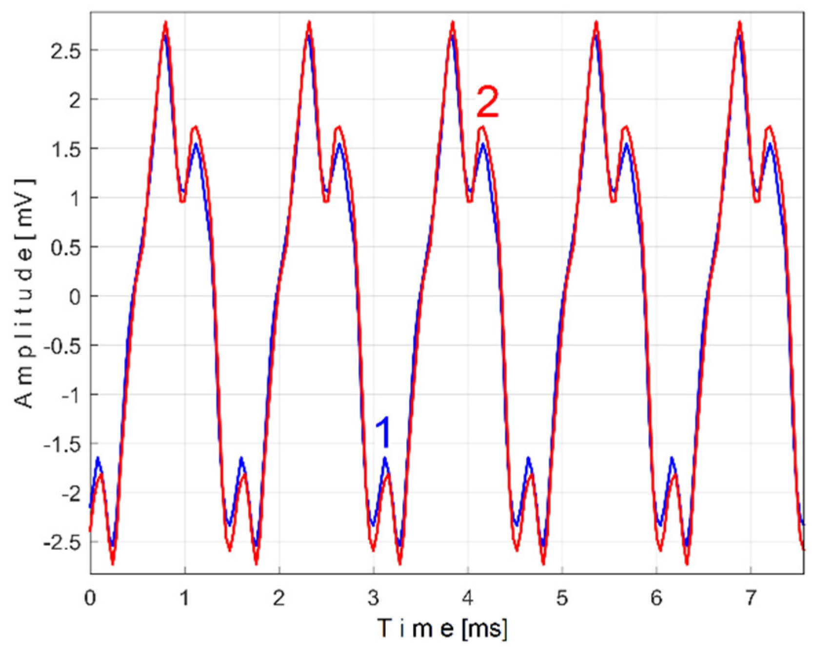
Figure 34.
The extended AMSSRTI patterns (m = 3250) describing the behavior of component TVC58 in signal sV: 1 –sVTC58e5a, fVC58a = 797.5646 Hz; 2 - sVTC58e5b, fVC58b = 798.1551Hz.
Figure 34.
The extended AMSSRTI patterns (m = 3250) describing the behavior of component TVC58 in signal sV: 1 –sVTC58e5a, fVC58a = 797.5646 Hz; 2 - sVTC58e5b, fVC58b = 798.1551Hz.
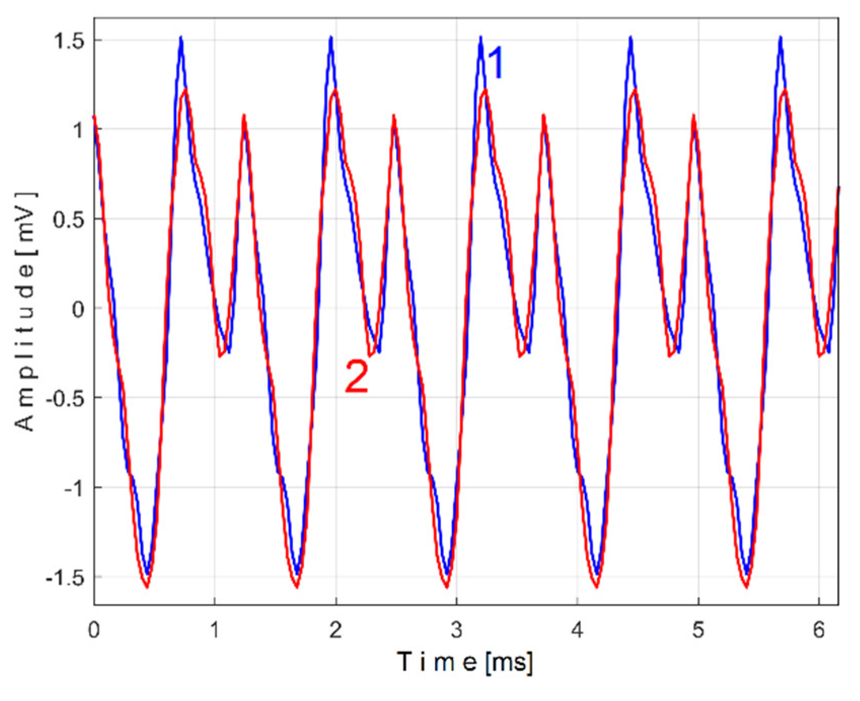
Figure 35.
shows the pattern for m = 65,700 (as sVTC48e5a) from the analysis of almost 2.5 Ms from signal sV (with fVC48a = 660.19726 Hz). Curve 4 shows the pattern for m = 65,700 (as sVTC48e5b) from the analysis of the next almost 2.5 Ms from signal sV (with fVC48b = 660.58252 Hz).
Figure 35.
shows the pattern for m = 65,700 (as sVTC48e5a) from the analysis of almost 2.5 Ms from signal sV (with fVC48a = 660.19726 Hz). Curve 4 shows the pattern for m = 65,700 (as sVTC48e5b) from the analysis of the next almost 2.5 Ms from signal sV (with fVC48b = 660.58252 Hz).
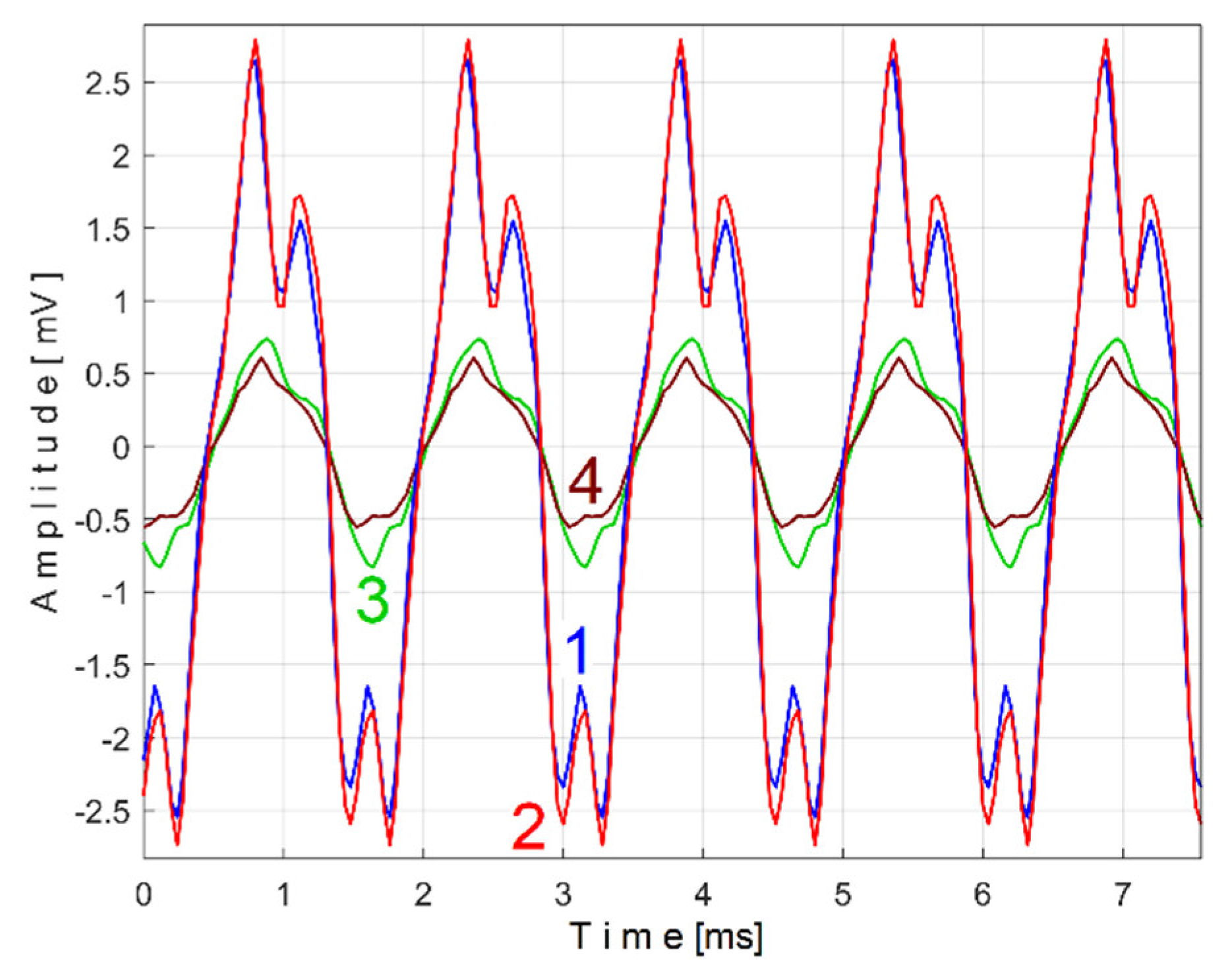
Figure 36.
The unfiltered extended AMSSRTI patterns (m = 2155) which describes the behaviour of shaft I in signal sV: 1 - sVTCe5a, fVDa = 21.56087 Hz; 2 - sVTDe5b, fVDb = 21.57886 Hz.
Figure 36.
The unfiltered extended AMSSRTI patterns (m = 2155) which describes the behaviour of shaft I in signal sV: 1 - sVTCe5a, fVDa = 21.56087 Hz; 2 - sVTDe5b, fVDb = 21.57886 Hz.
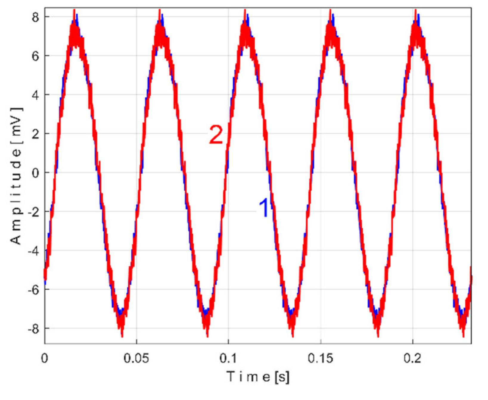
Figure 37.
The low-pass filtered extended patterns from Figure 36.
Figure 37.
The low-pass filtered extended patterns from Figure 36.
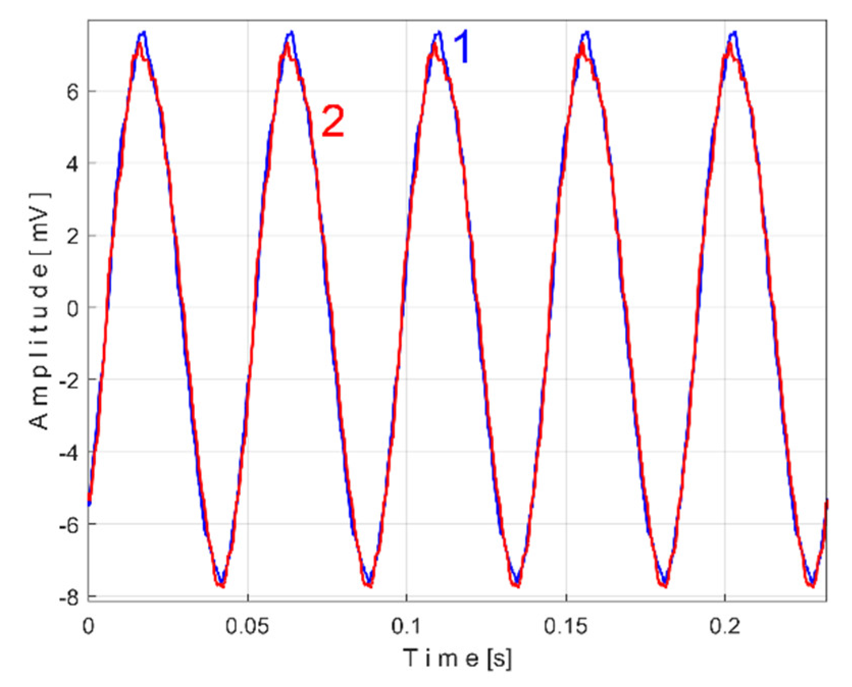
Figure 38.
The time-domain representation of IAS of spindle during 10 s of steady-state regime.
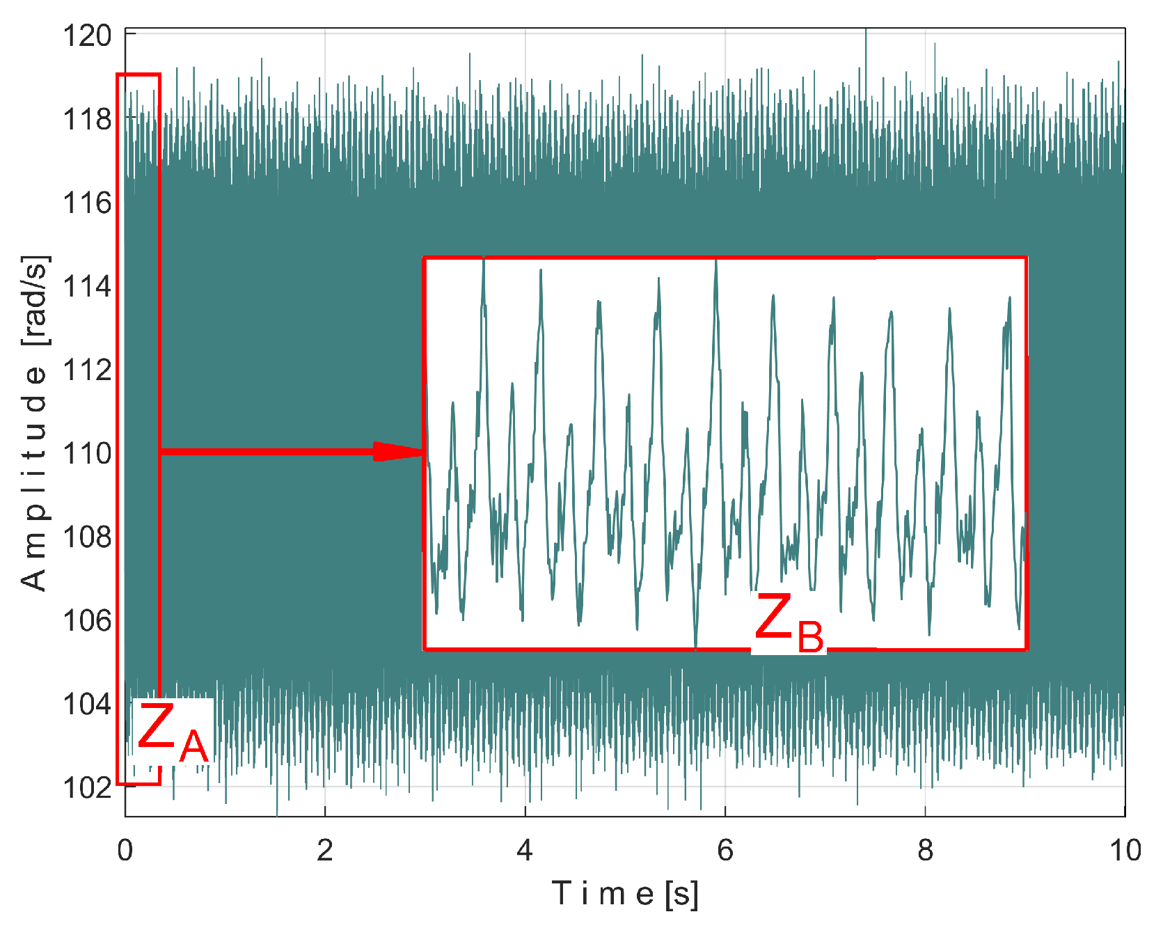
Figure 39.
The time-domain representation of variable part of the filtered IAS (sI) from Figure 38.
Figure 39.
The time-domain representation of variable part of the filtered IAS (sI) from Figure 38.
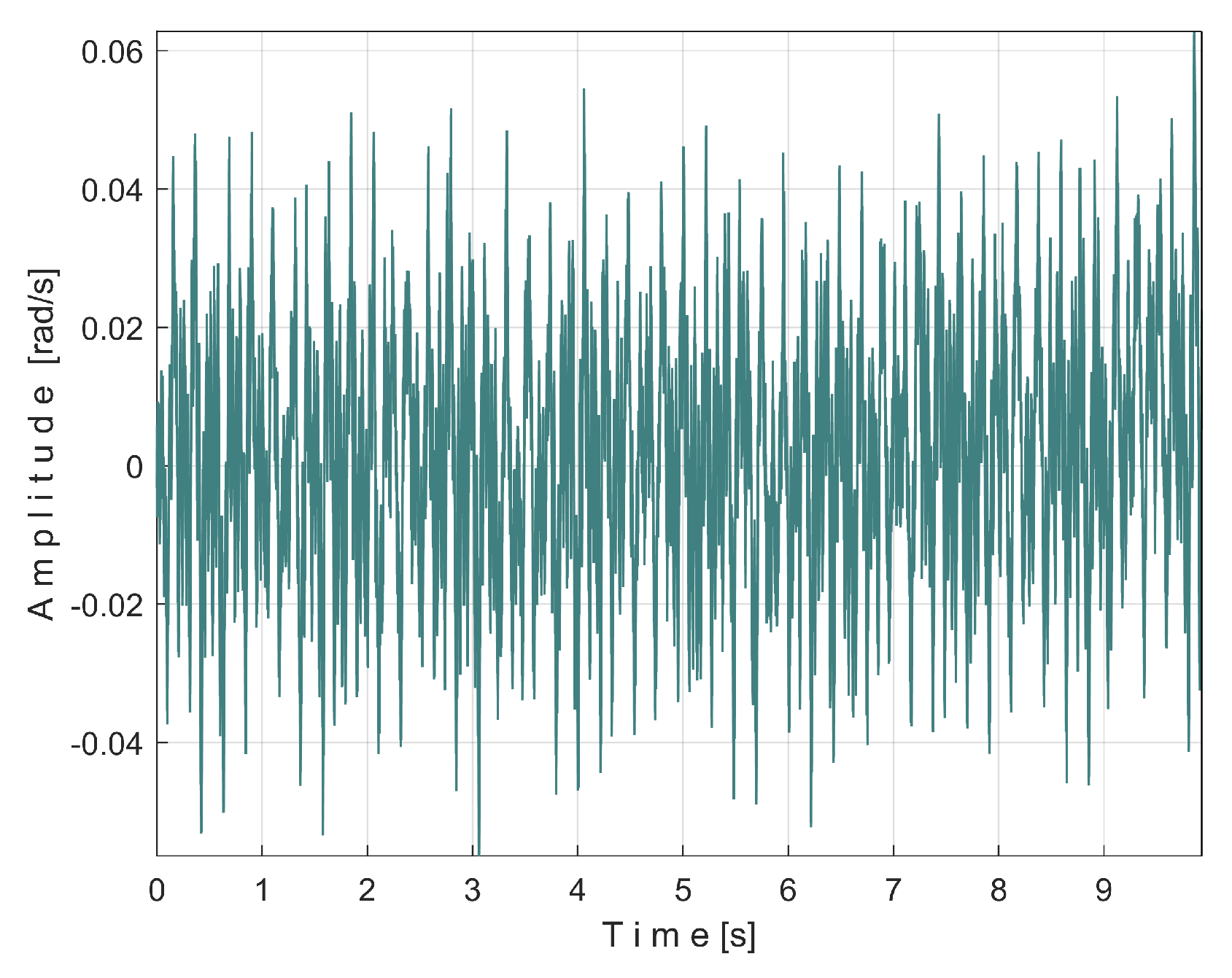
Figure 40.
The partial FFT spectrum of signal sI (0÷40 Hz range).
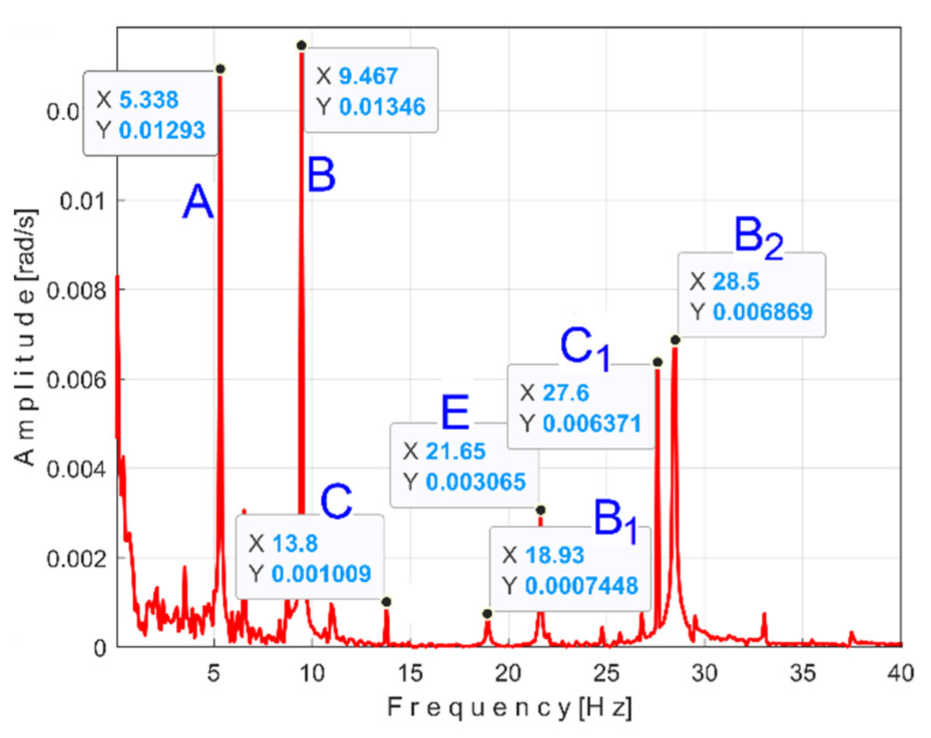
Figure 41.
The unfiltered extended AMSSRTI patterns (m = 25) describing the behaviour of the first flat belt in signal sI: 1 – sITAe5a, fIAa = 5.40021 Hz; 2 – sITAe5b, fIAb = 5.4107 Hz.
Figure 41.
The unfiltered extended AMSSRTI patterns (m = 25) describing the behaviour of the first flat belt in signal sI: 1 – sITAe5a, fIAa = 5.40021 Hz; 2 – sITAe5b, fIAb = 5.4107 Hz.
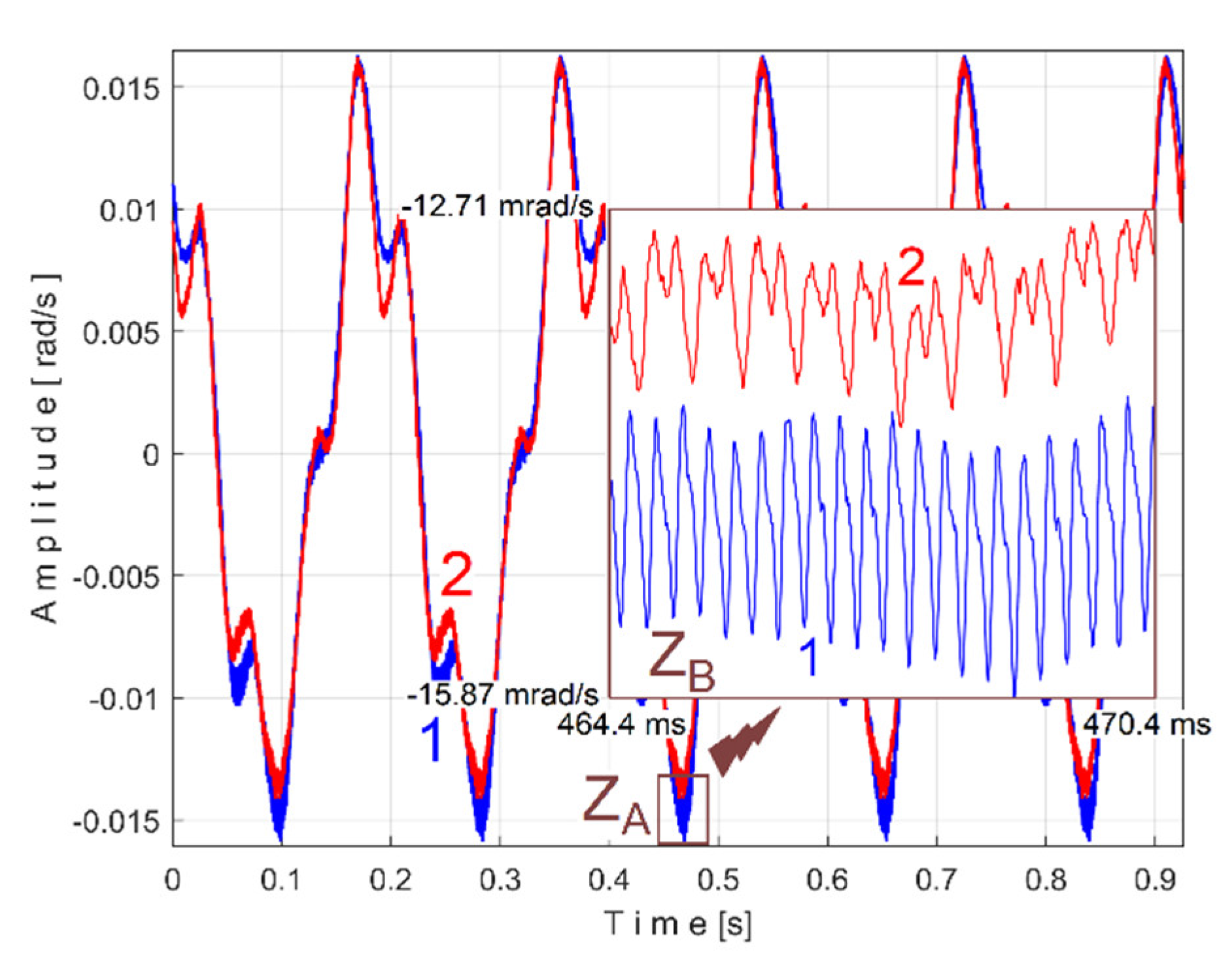
Figure 42.
The unfiltered extended AMSSRTI patterns (m = 46) describing the behaviour of the second flat belt in signal sI: 1 – sITBe5a, fIBa = 9.48999 Hz; 2 – sITBe5b, fIBb = 9.49061 Hz.
Figure 42.
The unfiltered extended AMSSRTI patterns (m = 46) describing the behaviour of the second flat belt in signal sI: 1 – sITBe5a, fIBa = 9.48999 Hz; 2 – sITBe5b, fIBb = 9.49061 Hz.
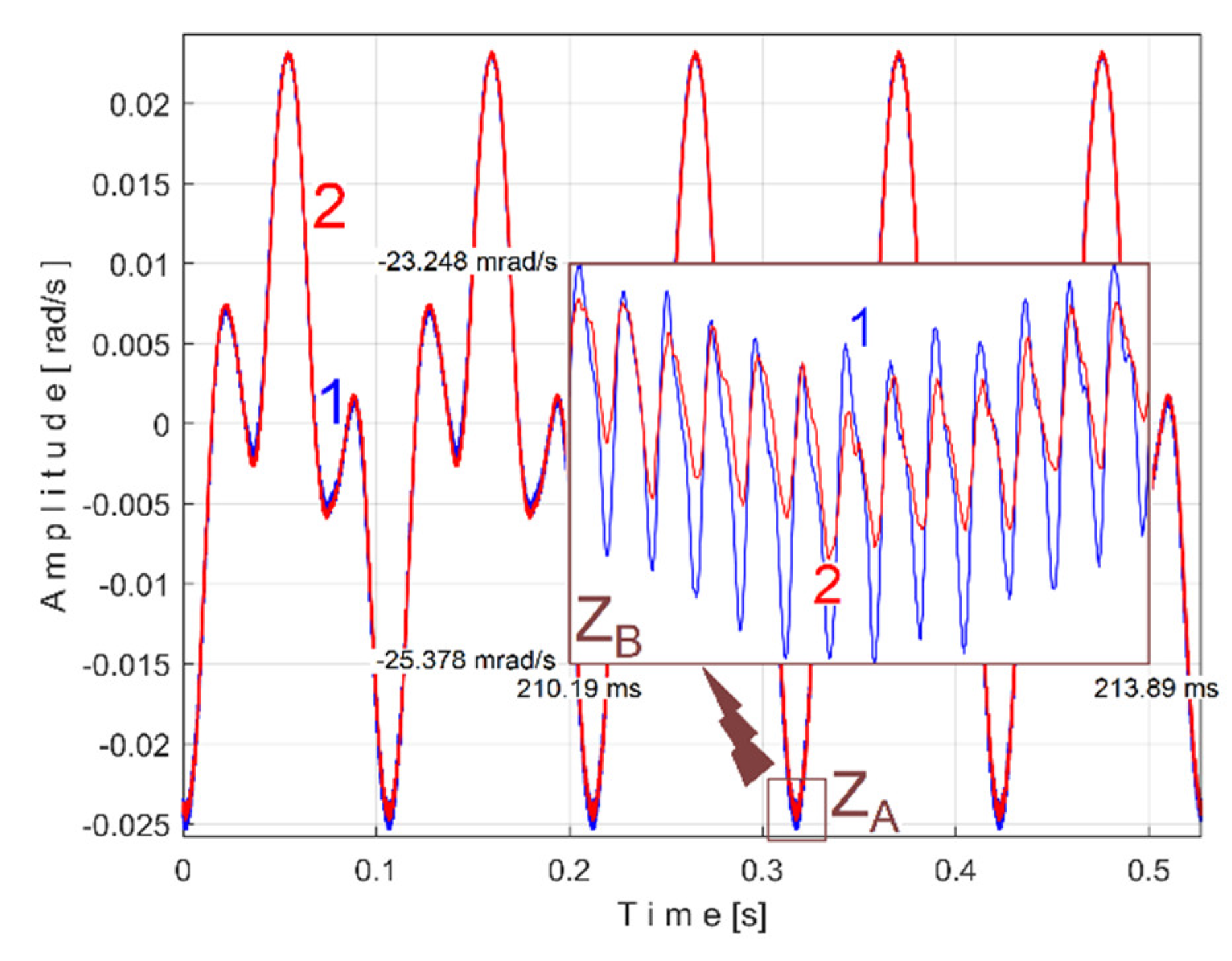
Figure 43.
The unfiltered extended AMSSRTI patterns (m = 17,100) of the false variable component with periods TIBa369 and TIBb369 in signal sI: 1 – sITB369e5a, fIB369a = 3501.7959 Hz; 2 – sITB369e5b, fIB369b = 3501.7417 Hz.
Figure 43.
The unfiltered extended AMSSRTI patterns (m = 17,100) of the false variable component with periods TIBa369 and TIBb369 in signal sI: 1 – sITB369e5a, fIB369a = 3501.7959 Hz; 2 – sITB369e5b, fIB369b = 3501.7417 Hz.
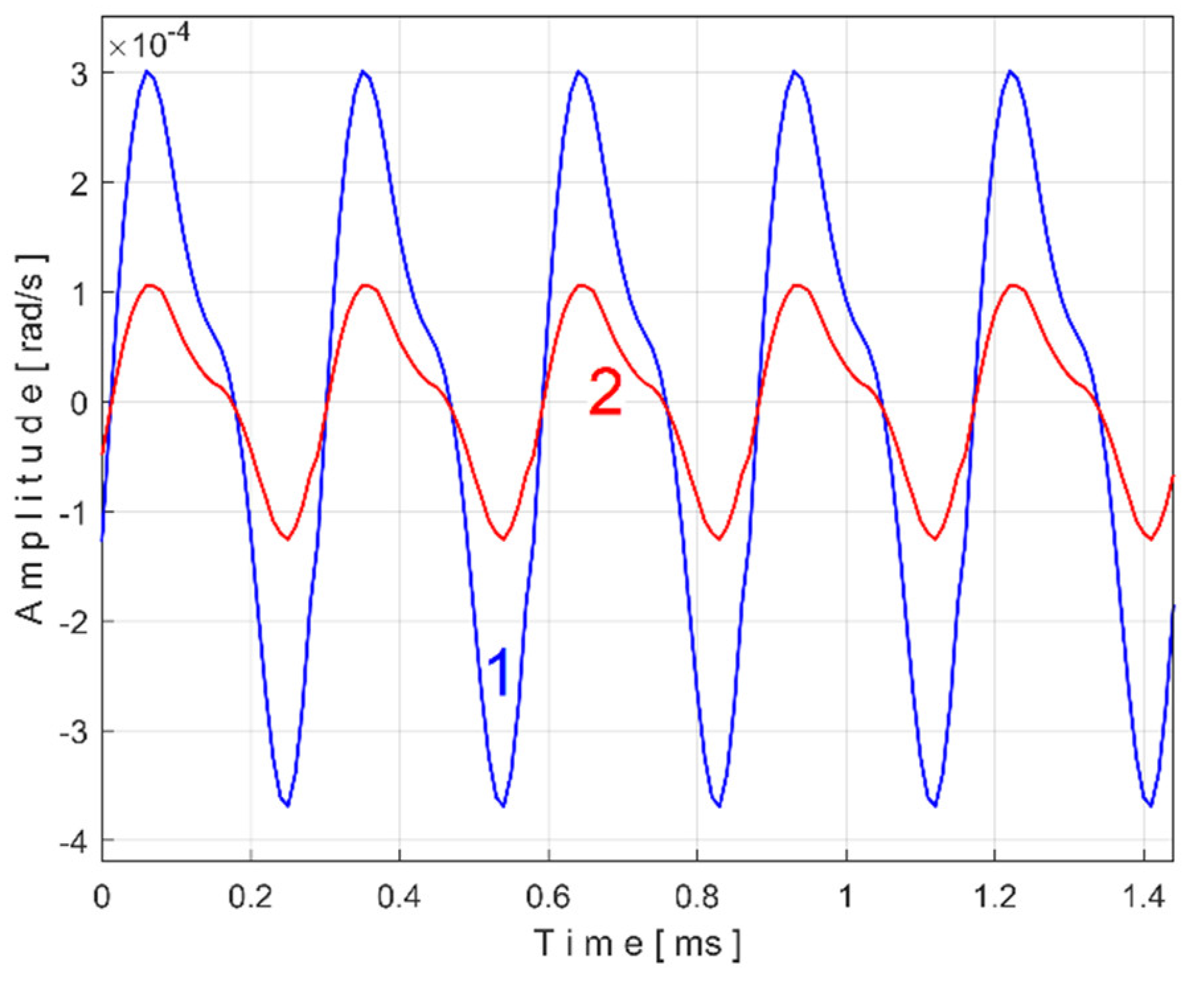
Figure 44.
The unfiltered extended AMSSRTI patterns (m = 68) describing the behaviour of the shaft I in signal sI: 1 – sITCe5a, fICa = 13.826942 Hz; 2 – sITCe5b, fICb = 13.79066 Hz.
Figure 44.
The unfiltered extended AMSSRTI patterns (m = 68) describing the behaviour of the shaft I in signal sI: 1 – sITCe5a, fICa = 13.826942 Hz; 2 – sITCe5b, fICb = 13.79066 Hz.
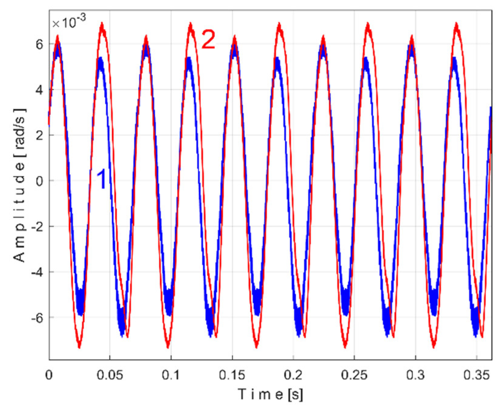
Figure 45.
The unfiltered extended AMSSRTI patterns (m = 106) describing the behaviour of the shaft II in signal sI: 1 – sITEe5a, fIEa = 21.6422 Hz; 2 – sITEe5b, fIEb = 21.64315 Hz.
Figure 45.
The unfiltered extended AMSSRTI patterns (m = 106) describing the behaviour of the shaft II in signal sI: 1 – sITEe5a, fIEa = 21.6422 Hz; 2 – sITEe5b, fIEb = 21.64315 Hz.
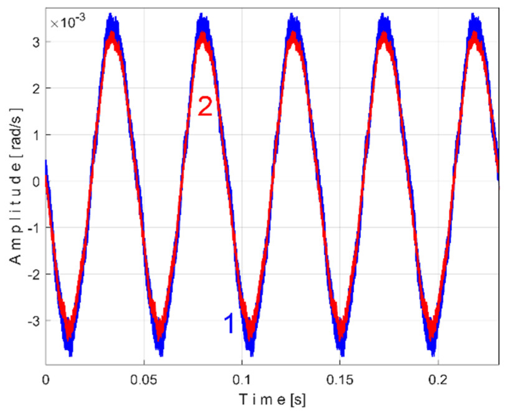
Figure 46.
The influence of frequency (period) variation on AMSSRTI extended pattern sPTAe5a shape (from Figure 15, m = 530): 1- sPTAe5a (correct frequency fPAa = 5.33748 Hz); 2- sPTAe5a- (deliberately wrong, very slightly lower frequency fPAa- = 5.335 Hz = fPAa - 0.00248 Hz); 3 - sPTAe5a+ (deliberately wrong, very slightly higher frequency fPAa+ = 5.339 Hz = fPAa + 0.00152 Hz).
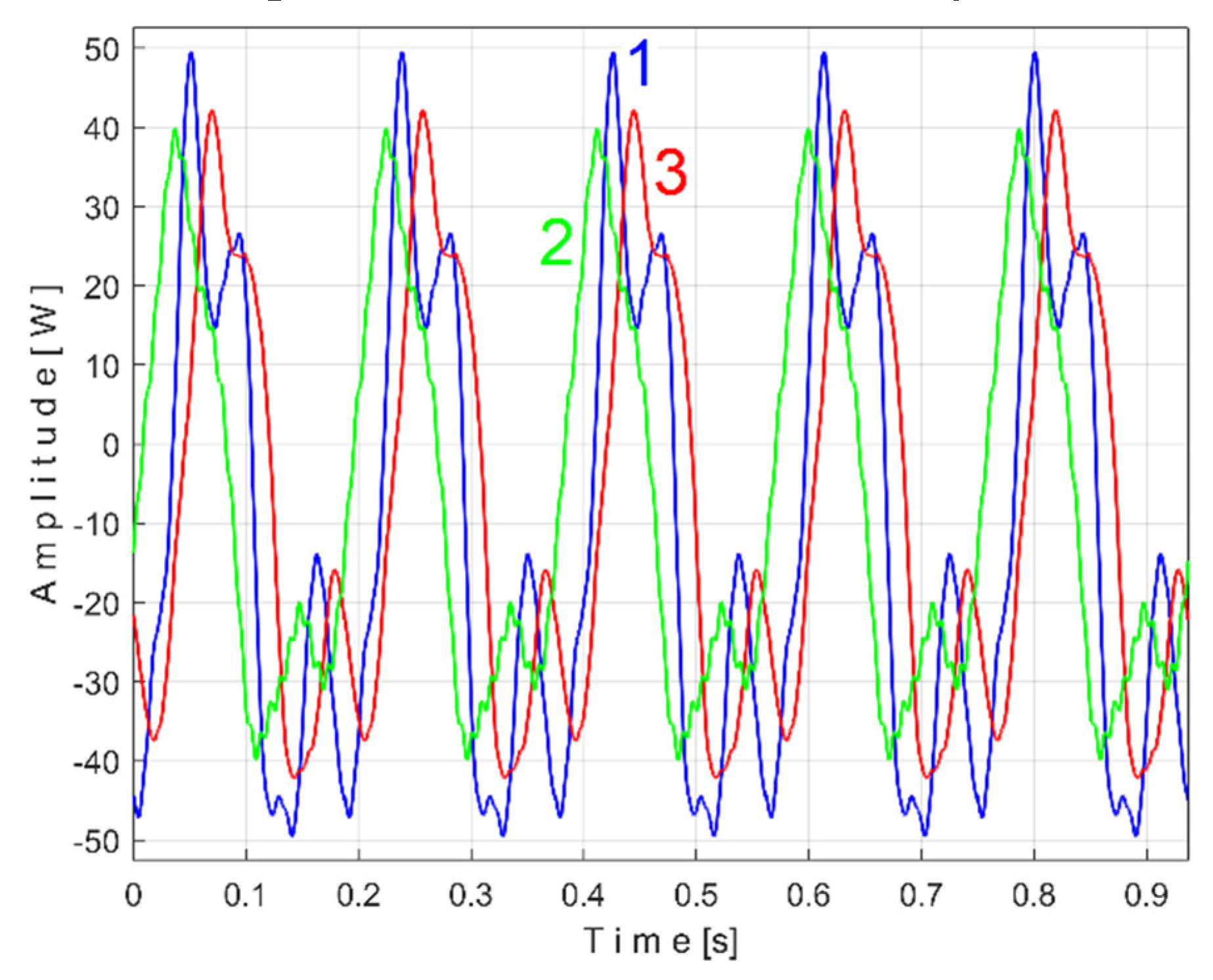
Figure 51.
The extended AMSSRTI patterns describing the behaviour of the shaft III and spindle in signal sP (using small values of m): 1 - sPTDe5a1 (m=20, fPDa1 = 17.35793 Hz); 2 – sPTDe5a2 (m=100, fPDa2 = 17.3638 Hz).
Figure 51.
The extended AMSSRTI patterns describing the behaviour of the shaft III and spindle in signal sP (using small values of m): 1 - sPTDe5a1 (m=20, fPDa1 = 17.35793 Hz); 2 – sPTDe5a2 (m=100, fPDa2 = 17.3638 Hz).
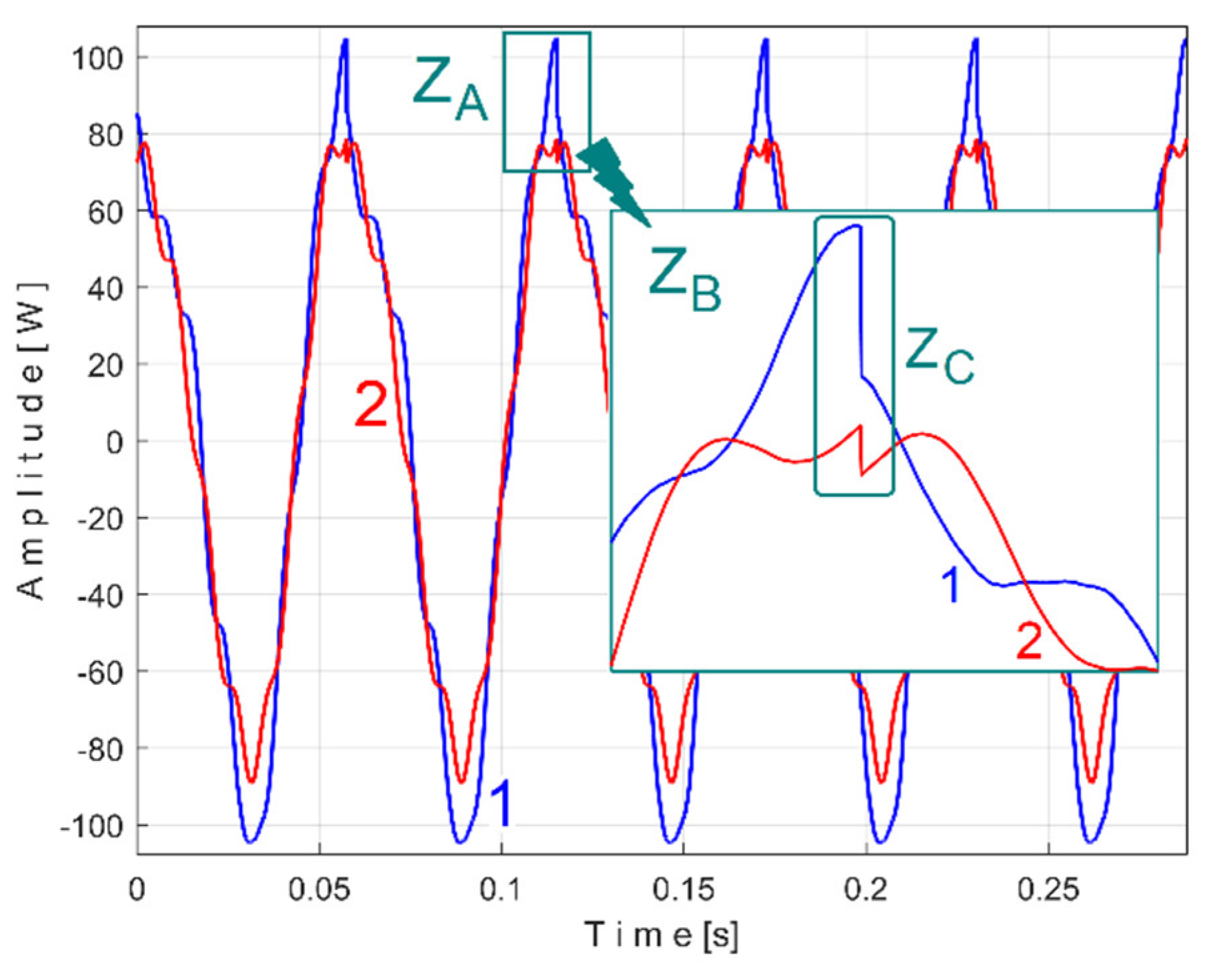

Table 1.
The average values of frequency of peaks (describing the fundamental of periodic components) A ÷ E.
Table 1.
The average values of frequency of peaks (describing the fundamental of periodic components) A ÷ E.
| fPA [Hz] | fPB [Hz] | fPC [Hz] | fPD [Hz] | fPE [Hz] | |
| Found using FFT | 5.342 | 9.454 | 13.76 | 17.38 | 21.58 |
| Found using AMSSRTI |
5.3408 (m = 1061) |
9.4589 (m = 1872) |
13.76513 (m = 2728 |
17.3865 (m = 3453) |
21.5761 (m = 4288) |
Table 2.
The amplitudes, frequencies and phases at the origin of time for the sinusoidal components involved (by addition) in the description of the variable part of the active electrical power generated by the first flat belt.
Table 2.
The amplitudes, frequencies and phases at the origin of time for the sinusoidal components involved (by addition) in the description of the variable part of the active electrical power generated by the first flat belt.
| FPA | HPA1 | HPA2 | HPA3 | HPA4 | HPA5 | HPA6 | HPA8 | |
| Amplitude [W] | 37.19 | 15.33 | 15.5 | 6.268 | 8.482 | 2.157 | 4.499 | 0.446 |
| Frequency [Hz] | 5.341 | 10.684 | 16.026 | 21.374 | 26.706 | 32.053 | 37.401 | 48.080 |
| Phase at origin of time [rad] | 0.9581 | 0.1707 | 2.359 | 1.204 | 0.5218 | 2.307 | 1.266 | -1.863 |
Disclaimer/Publisher’s Note: The statements, opinions and data contained in all publications are solely those of the individual author(s) and contributor(s) and not of MDPI and/or the editor(s). MDPI and/or the editor(s) disclaim responsibility for any injury to people or property resulting from any ideas, methods, instructions or products referred to in the content. |
© 2025 by the authors. Licensee MDPI, Basel, Switzerland. This article is an open access article distributed under the terms and conditions of the Creative Commons Attribution (CC BY) license (http://creativecommons.org/licenses/by/4.0/).
Copyright: This open access article is published under a Creative Commons CC BY 4.0 license, which permit the free download, distribution, and reuse, provided that the author and preprint are cited in any reuse.


