
Submitted:
03 January 2025
Posted:
07 January 2025
You are already at the latest version
Abstract
This study is aimed at a comprehensive assessment of the chemical composition of surface waters in the Turkestan region and their impact on regional landscapes. The primary objective of the research is to systematically evaluate the level of chemical pollution in the region's water resources and determine its indirect effects on landscape-ecological stability. In August 2024, water samples from eight sampling points (S1–S8) were analyzed for 24 physicochemical parameters, including total hardness (mg*eq/L), pH, dry residue (mg/L), electrical conductivity (µS/cm), total salinity (mg/L), Al, As, B, Ca, Cd, Co, Cr, Ti, Fe, Pb, Cu, Mg, K, Mn, Na, Ni, Zn, SO₄²⁻, and C₆H₅OH. To determine the degree of pollution, variational-statistical analysis, principal component analysis (PCA), as well as the calculation of the OIP, NPI, and HPI indices were performed. For land use and land cover change (LULC) analysis, LULC classification was carried out based on Landsat data from 2000 to 2020, forming the basis for land resource management and planning. The research results showed a deterioration in the ecological condition of water resources and an increasing anthropogenic impact. Specifically, at point S8, the concentration of Al was found to be 56 times higher than the maximum allowable limit, while the concentration of Fe was 42 times higher. High levels of pollution were also recorded at points S1, S4, S5, and S6, where the increase in Al and Na concentrations caused a sharp rise in the OIP value. The main factors influencing water pollution include industrial effluents, agricultural waste, and irrigation drainage waters. The pollution's negative impact on regional landscapes has led to issues related to the distribution of vegetation, soil fertility, and landscape stability. To improve the current ecological situation and restore natural balance, the phytoremediation method is proposed. The research results will serve as the foundation for developing water resource management strategies for the Turkestan region and making informed decisions aimed at ensuring ecological sustainability.
Keywords:
1. Introduction
- Evaluate water quality based on chemical parameters obtained from various sampling points;
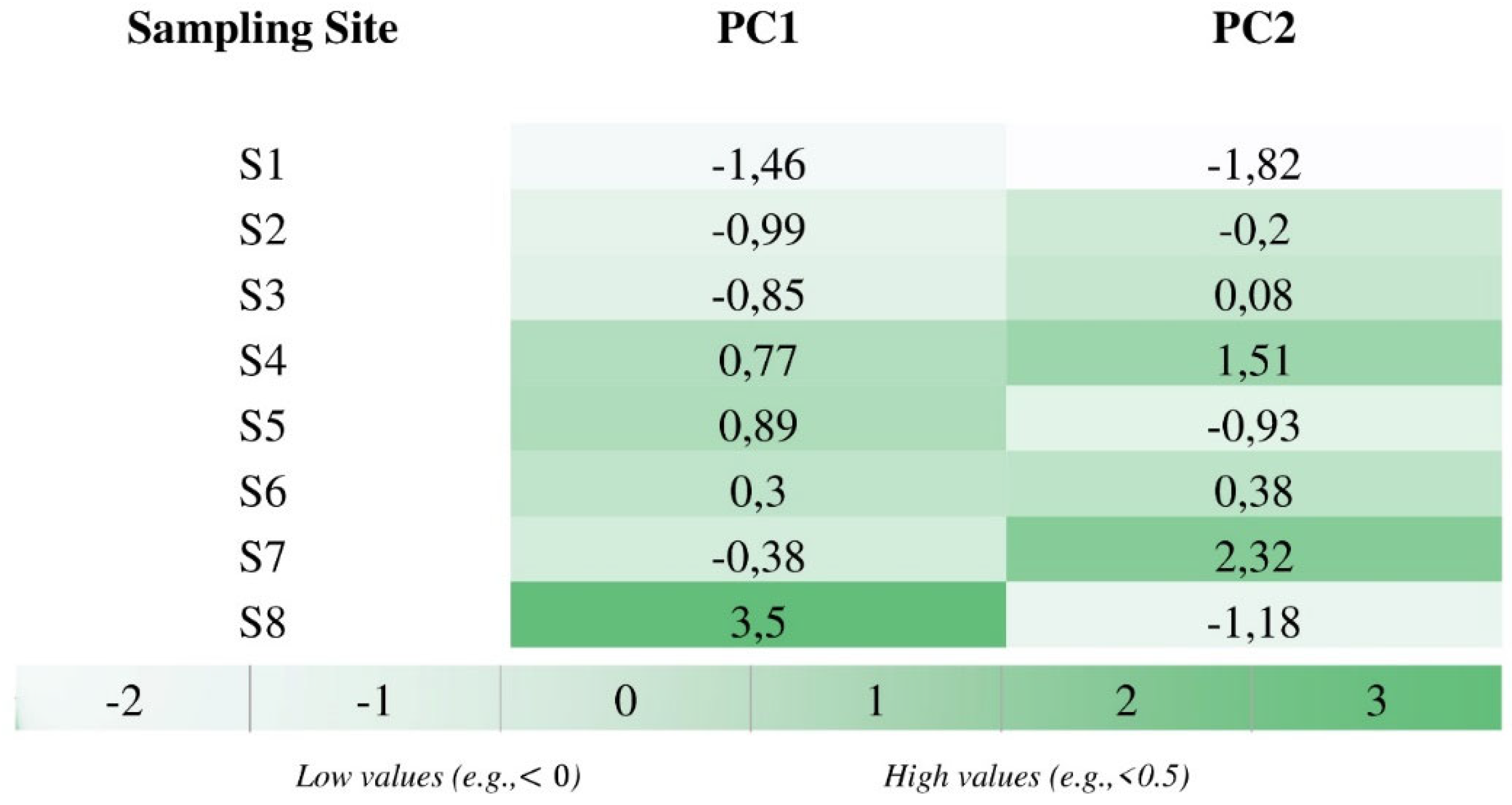
- Perform variational-statistical analysis, principal component analysis (PCA), and calculate the OIP, NPI, and HPI indices to determine the pollution level;
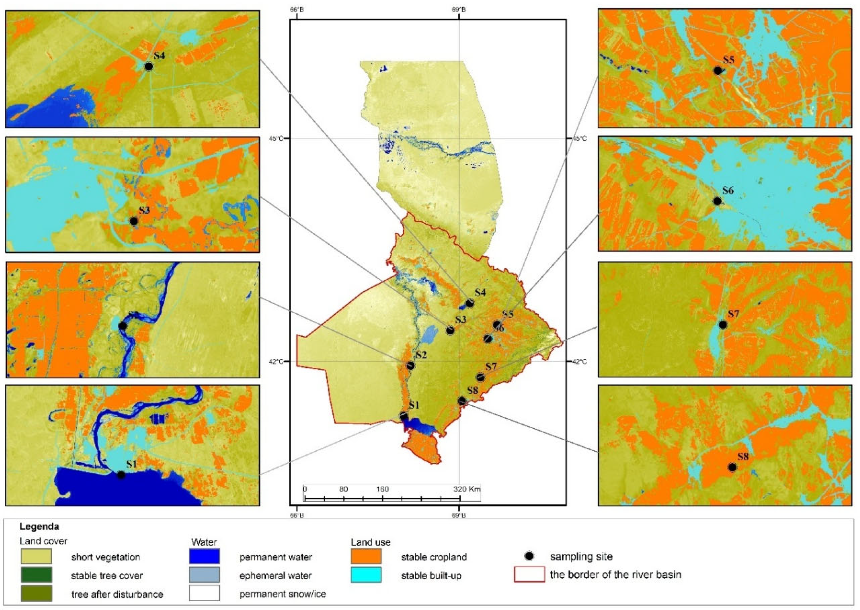
- Identify land use and land cover changes (LULC);
- Apply statistical methods to explore the relationships between water quality and land use;
2. Materials and Methods
2.1. Study Area
2.2. Water Sampling and Analytical Methods
2.3. Variational-Statistical Analysis
2.4. Water Quality Analysis:
2.4.1. Overall Pollution Index (OIP)
2.4.2. Nemerov’s Pollution Index (NPI)
2.4.3. Heavy Metal Pollution Index (HPI)
2.5. Land Use and Land Cover (LULC) Classification
3. Results and Discussion
3.1. Physicochemical Indicators of Surface Waters in the Turkestan Region
3.2. Water Quality Analysis:
3.2.1. Water Quality Analysis Through the Overall Pollution Index (OIP)
3.2.2. Analysis Using Nemerov’s Pollution Index (NPI):
3.2.3. Heavy Metal Pollution Index (HPI)
3.3. Land Use Changes and Water Quality
3.4. Indirect Effects of Chemical Pollution Load in Surface Waters on Landscapes
3.5. Water Pollution’s Impact on Local Hydrological Cycles and Landscapes
3.6. Purification of River Water Contaminated with Heavy Metals
- Accumulation of pollutants (phytoextraction and rhizofiltration),
- Immobilization of pollutants (phytostabilization),
- Biodegradation (rhizodegradation and phytodegradation),
- Dissipation (phytovolatilization).
- Continuous Water Quality Monitoring: Use sensors to monitor the dynamics of heavy metals.
- Adaptation of Local Plant Species: Utilize plants adapted to the local climatic conditions.
- Recycling Plant Biomass: Use the biomass obtained after purification as a source of bioenergy.
- Conduct Additional Scientific Research: Continue research to find effective solutions adapted to different ecosystems.
- These recommendations will allow for the ecological, safe, and sustainable restoration of the water resources in the Turkestan region.
4. Conclusions
Author Contributions
Funding
Data Availability Statement
Acknowledgments
Conflicts of Interest
References
- Bunn, S.E.; Davies, P.M.; Mosisch, T.D. Ecosystem measures of river health and their response to riparian and catchment degradation. Freshwater Biology 1999, 41(2), 333–345. [Google Scholar] [CrossRef]
- Newson, M. Understanding ’hot-spot’ problems in catchments: The need for scale-sensitive measures and mechanisms to secure effective solutions for river management and conservation. Aquatic Conservation: Marine and Freshwater Ecosystems 2010, 20(Supplement 1), S62–S72. [CrossRef]
- Guermazi, E.; Milano, M.; Reynard, E.; et al. Impact of climate change and anthropogenic pressure on the groundwater resources in arid environment. Mitigation and Adaptation Strategies for Global Change 2019, 24, 73–92. [Google Scholar] [CrossRef]
- Bracken, L.J.; Croke, J. The concept of hydrological connectivity and its contribution to understanding runoff-dominated geomorphic systems. Hydrological Processes 2007, 21(13), 1749–1763. [Google Scholar] [CrossRef]
- Fernandes, A.C.P.; de Oliveira Martins, L.M.; Pacheco, F.A.L.; Fernandes, L.F.S. The consequences for stream water quality of long-term changes in landscape patterns: Implications for land use management and policies. Land Use Policy 2021, 109, 105679. [Google Scholar] [CrossRef]
- Ba, W.; Du, P.; Liu, T.; Bao, A.; Chen, X.; Liu, J.; Qin, C. Impacts of climate change and agricultural activities on water quality in the Lower Kaidu River Basin, China. Journal of Geographical Sciences 2020, 30(1), 164–176. [Google Scholar] [CrossRef]
- Alamri, D.A.; Al-Solaimani, S.G.; Abohassan, R.A.; Rinklebe, J.; Shaheen, S.M. Assessment of water contamination by potentially toxic elements in mangrove lagoons of the Red Sea, Saudi Arabia. Environmental Geochemistry and Health 2021, 43(11), 4819–4830. [Google Scholar] [CrossRef]
- Quan, J.; Xu, Y.; Ma, T.; Wilson, J.P.; Zhao, N.; Ni, Y. Improving surface water quality of the Yellow River Basin due to anthropogenic changes. Science of the Total Environment 2022, 836, 155607. [Google Scholar] [CrossRef]
- Hussein, A. Impacts of land use and land cover change on vegetation diversity of tropical highland in Ethiopia. Applied Environmental Soil Science 2023, 2023, 1–11. [Google Scholar] [CrossRef]
- Pandey, P.C.; Koutsias, N.; Petropoulos, G.P.; Srivastava, P.K.; Ben Dor, E. Land use/land cover in view of earth observation: Data sources, input dimensions, and classifiers—A review of the state of the art. Geocarto International 2021, 36(10), 957–988. [Google Scholar] [CrossRef]
- Chaemiso, S.E.; Kartha, S.A.; Pingale, S.M. Effect of land use/land cover changes on surface water availability in the Omo Gibe basin, Ethiopia. Hydrological Sciences Journal 2021, 66(12), 1936–1962. [Google Scholar] [CrossRef]
- Emenike, P.C.; et al. An integrated assessment of land-use change impact, seasonal variation of pollution indices and human health risk of selected toxic elements in sediments of River Atuwara, Nigeria. Environmental Pollution 2020, 265, 114795. [Google Scholar] [CrossRef] [PubMed]
- Phanmala, K.; Lai, Y.; Xiao, K. Impact of land use change on the water environment of a key marsh area in Vientiane Capital, Laos. Water 2023, 15(21), 4302. [Google Scholar] [CrossRef]
- Qiu, Z.; Kennen, J.G.; Giri, S.; Walter, T.; Kang, Y.; Zhang, Z. Reassessing the relationship between landscape alteration and aquatic ecosystem degradation from a hydrologically sensitive area perspective. Science of the Total Environment 2019, 650(Part 2), 2850–2862. [Google Scholar] [CrossRef]
- Bhat, S.U.; Khanday, S.A.; Islam, S.T.; Sabha, I. Understanding the spatiotemporal pollution dynamics of highly fragile montane watersheds of Kashmir Himalaya, India. Environmental Pollution 2021, 286, 117335. [Google Scholar] [CrossRef] [PubMed]
- Mello, K.D.; Taniwaki, R.H.; Paula, F.R.D.; Valente, R.A.; Randhir, T.O.; Macedo, D.R.; Leal, C.G.; Hughes, R.M. Multiscale land use impacts on water quality: Assessment, planning, and future perspectives in Brazil. Journal of Environmental Management 2020, 270, 110879. [Google Scholar] [CrossRef]
- Ma, B.; Wu, C.; Jia, X.; Zhang, Y.; Zhou, Z. Predicting water quality using partial least squares regression of land use and morphology (Danjiangkou Reservoir, China). Journal of Hydrology 2023, 624, 129828. [Google Scholar] [CrossRef]
- Mitchell, M.G.E.; Bennett, E.M.; Gonzalez, A. Linking Landscape Connectivity and Ecosystem Service Provision: Current Knowledge and Research Gaps. Ecosystems 2013, 16(5), 894–908. [Google Scholar] [CrossRef]
- Zhang, J.; Li, S.; Dong, R.; Jiang, C.; Ni, M. Influences of land use metrics at multi-spatial scales on seasonal water quality: A case study of river systems in the Three Gorges Reservoir Area, China. Journal of Cleaner Production 2019, 206, 76–85. [Google Scholar] [CrossRef]
- Abazeri, M. Women of the Sun: Mediating Co-Production in Iranian Agrarian Systems. University of Miami, 2023. Available online: https://scholarship.miami.edu/theses/5698.
- Mrabet, R. Sustainable agriculture for food and nutritional security. In Sustainable Agriculture and the Environment; Mrabet, R., Ed.; Elsevier: 2023; pp. 25–90.
- Nwachukwu, B.C. Microbial Diversity, Community Structure and Functional Characteristics of Sunflower Rhizospheric Soil. Ph.D. Thesis, North-West University, South Africa, 2023. [Google Scholar]
- Ding, J.; Jiang, Y.; Liu, Q.; Hou, Z.; Liao, J.; Fu, L.; Peng, Q. Influences of the land use pattern on water quality in low-order streams of the Dongjiang River basin, China: A multi-scale analysis. Science of the Total Environment 2016, 551–552, 205–216. [CrossRef]
- Barroso, G.R.; Pinto, C.C.; Gomes, L.N.L.; Oliveira, S.C. Assessment of water quality based on statistical analysis of physical chemical, biomonitoring and land use data: Manso River supply reservoir. Science of the Total Environment 2024, 912, 169554. [Google Scholar] [CrossRef]
- Chattopadhayay, R.; Ghosh, A.K. Performance appraisal based on a forced distribution system: Its drawbacks and remedies. International Journal of Productivity and Performance Management 2012, 61(8), 881–896. [Google Scholar] [CrossRef]
- Uddin, M.G.; Nash, S.; Olbert, A.I. A review of water quality index models and their use for assessing surface water quality. Ecological Indicators 2021, 122, 107218. [Google Scholar] [CrossRef]
- Dawood, A.S. Using of Nemerow’s Pollution Index (NPI) for water quality assessment of some Basrah Marshes, South of Iraq. Journal of Babylon University for Pure and Applied Sciences 2017, 25(5), 1708–1720. [Google Scholar]
- Subagiyo, L.; Nuryadin, A.; Sulaeman, N.F.; Widyastuti, R. Water quality status of Kalimantan water bodies based on the pollution index. Pollution Research 2019, 38(3), 536–543. [Google Scholar]
- Hu, B.; et al. Current status, spatial features, health risks, and potential driving factors of soil heavy metal pollution in China at province level. Environmental Pollution 2020, 266, 114961. [Google Scholar] [CrossRef] [PubMed]
- Mitra, S.; et al. Impact of heavy metals on the environment and human health: Novel therapeutic insights to counter the toxicity. Journal of King Saud University - Science 2022, 34(6), 101865. [CrossRef]
- Munir, N.; et al. Heavy metal contamination of natural foods is a serious health issue: A review. Sustainability 2021, 14(1), 161. [Google Scholar] [CrossRef]
- Sharma, R.; Agrawal, P.R.; Kumar, R.; Gupta, G. Current scenario of heavy metal contamination in water. In Contaminants in Water; Elsevier: 2021; pp. 49–64.
- Zaynab, M.; et al. Health and environmental effects of heavy metals. Journal of King Saud University - Science 2022, 34(6), 101653.
- Ali, M.M.; et al. Environmental pollution with heavy metals: A public health concern. In Heavy Metals - Their Environmental Impacts and Mitigation; Springer: 2021; pp. 771–783.
- Authman, M.M.; Zaki, M.S.; Khallaf, E.A.; Abbas, H.H. Use of fish as bio-indicator of the effects of heavy metals pollution. Journal of Aquaculture Research and Development 2015, 6(2), 1–13. [Google Scholar] [CrossRef]
- Briffa, J.; Sinagra, E.; Blundell, R. Heavy metal pollution in the environment and their toxicological effects on humans. Heliyon 2020, 6(9), e04691. [Google Scholar] [CrossRef]
- Engwa, G.A.; Ferdinand, P.U.; Nwalo, F.N.; Unachukwu, M.N. Mechanism and health effects of heavy metal toxicity in humans. In Poisoning in the Modern World - New Tricks for an Old Dog; IntechOpen: 2019; pp. 70–90. [CrossRef]
- Patel, N.; et al. Contamination and health impact of heavy metals. In Water Pollution and Remediation: Heavy Metals; Springer International Publishing: 2021; pp. 259–280.
- Ustaoğlu, F.; Tepe, Y.; Aydin, H. Heavy metals in sediments of two nearby streams from Southeastern Black Sea coast: Contamination and ecological risk assessment. Environmental Forensics 2020, 21(2), 145–156. [Google Scholar] [CrossRef]
- Ustaoğlu, F.; Taş, B.; Tepe, Y.; Topaldemir, H. Comprehensive assessment of water quality and associated health risk by using physicochemical quality indices and multivariate analysis in Terme River, Turkey. Environmental Science and Pollution Research 2021, 28(47), 62736–62754. [Google Scholar] [CrossRef]
- Egbueri, J. C., & Unigwe, C. O. (2020). Understanding the extent of heavy metal pollution in drinking water supplies from Umunya, Nigeria: An indexical and statistical assessment. Analytical Letters, 53(13), 2122–2144.
- Kumar, V., et al. (2019). Global evaluation of heavy metal content in surface water bodies: A meta-analysis using heavy metal pollution indices and multivariate statistical analyses. Chemosphere, 236, 124364. [CrossRef]
- OKG.KZ. (2024). Implementation of water-saving technology – an urgent matter [Internet resource]. Available online: https://okg.kz/post?id=35356&slug=su-unemdeu-tehnologiyasyn-engizu-kezek-kuttirmeitin-is (accessed on 11 October 2024).
- [Internet resource]. Available online: https://primeminister.kz/news/reviews/ekologiyalyk-bastamalar-zannamany-zhetildiru-zhane-memlekettik-koldau-sharalary-2020-zhyldyn-korytyndysy-boyynsha-kazakstannyn-geologiya-zhane-tabigi-resurstar-salasynyn-damuy-1813013 (accessed on 11 October 2024).
- Quality Kazakhstan. (2024). The issue of environmental pollution with wastewater and its solutions [Online]. Available online: https://standard.kz/kz/post/qorsagan-ortany-agyndy-sularmen-lastau-maselesi-zane-ony-sesu (accessed on 11 October 2024).
- Akhmetova, D. S., Ramazanova, N. E., Yeginbayeva, A. E., Kenzhebay, R. N. (2024). Pollution of the soil cover of Turkestan region landscapes due to the impact of anthropogenic factors. Geography and Water Resources, 3, 96–107. [CrossRef]
- Ogar, N. P. (2018). Project for the scientific substantiation of the expansion of the Syrdarya-Turkestan State Regional Natural Park. Center for Remote Sensing and GIS “Terra”, Almaty.
- Gorshkov, S. P. (1982). Exodynamic processes of developed territories. Moscow: Nedra. 286 p.
- Akhmetova, D., & Salkinbekkyzy, A. (2024). Anthropogenic impact on soil and vegetation in Turkistan region: Chemical composition and heavy metal contamination. Journal of the Geographical Institute “Jovan Cvijic”, SASA, 2024 OnLine-First Issue 00, Pages: 13-13. [CrossRef]
- Zhanar Ozgeldinova, Zhandos Mukayev, Nurgul Ramazanova, Assel Bektemirova, Altyn Zhanguzhina, & Meruyert Ulykpanova (2024). Spatial distribution of potentially toxic elements in soils and water bodies of the Kostanay region in Kazakhstan. Scottish Geographical Journal. [CrossRef]
- Approval of the unified system for water quality classification in the water bodies of the Republic of Kazakhstan. (2016). Adilet. Available online: https://adilet.zan.kz/kaz/docs/V1600014513.
- Sargaonkar, A., & Deshpande, V. (2003). Development of an Overall Index of Pollution for Surface Water Based on a General Classification Scheme in Indian Context. Environmental Monitoring and Assessment, 89, 43–67. [CrossRef]
- El Mountassir, O., Bahir, M., Ouazar, D., Chehbouni, A. & Carreira, P. M. (2022). Temporal and spatial assessment of groundwater contamination with nitrate using nitrate pollution index (NPI), groundwater pollution index (GPI), and GIS (case study: Essaouira basin, Morocco). Environmental Science and Pollution Research, 29, 17132–17149.
- Kumar, V.; et al. (2019). Global evaluation of heavy metal content in surface water bodies: A meta-analysis using heavy metal pollution indices and multivariate statistical analyses. Chemosphere, 236, 124364. [CrossRef]
- González, F. M., & Pacheco, F. J. (2022). The Global 2000-2020 Land Cover and Land Use Change Dataset Derived From the Landsat Archive: First Results. Frontiers in Remote Sensing, 3, Article 856903. [CrossRef]
- Debnath, J., Saha, S., Sharma, R., Tiwari, K. & Deka, P. Geospatial modeling to assess the past and future land use-land cover changes in the Brahmaputra Valley, NE India, for sustainable land resource management. Environmental Science and Pollution Research, 30(39), 106997–107020 (2023).
- Hama Aziz, K. H., Mustafa, F. S., Omer, K. M., Hama, S., Hamarawf, R. F., & Rahman, K. O. (2023). Heavy metal pollution in the aquatic environment: efficient and low-cost removal approaches to eliminate their toxicity: A review. RSC Advances, 13, 17595–17610. [CrossRef]
- Wong, C. S. C., Li, X. D., & Thornton, I. (2006). Urban environmental geochemistry of trace metals. Environmental Pollution, 142(1), 1–16. [CrossRef]
- Gong, C., et al. (2022). Spatial differentiation and influencing factor analysis of soil heavy metal content at town level based on geographic detector. Environmental Science, 43, 4566–4577. [CrossRef]
- Pham-Duc, B., Nguyen, H., & Nguyen-Quoc, H. (2025). Unveiling the research landscape of planetscope data in addressing earth-environmental issues: A bibliometric analysis. Earth Science Informatics, 18(1), 52. [CrossRef]
- Byers, E.N., Messer, T.L., Unrine, J., Agouridis, C., & Miller, D.N. (2025). The occurrence and persistence of surface water contaminants across different landscapes. Science of the Total Environment, 958, 177837. [CrossRef]
- Ferreira, V.R.S., Cunha, E.J., Calvão, L.B., Michelan, T.S., & Juen, L. (2024). Amazon streams impacted by bauxite mining present distinct local contributions to the beta diversity of aquatic insects, fish, and macrophytes. Science of the Total Environment, 955, 177292. [CrossRef]
- Miao, Z., Yu, H., Jiang, R., Wang, C., & Cao, J. (2024). Unveiling the lifeblood of cities: Identifying urban ecological networks from the perspective of biodiversity conservation. Science of the Total Environment, 955, 177055. [CrossRef]
- Mousavi, M., Emrani, J., Teleha, J.C., Shamshiripour, A., & Fini, E.H. (2024). Health risks of asphalt emission: State-of-the-art advances and research gaps. Journal of Hazardous Materials, 480, 136048. [CrossRef]
- Al-Raeei, M. (2024). Artificial intelligence for climate resilience: Advancing sustainable goals in SDGs 11 and 13 and its relationship to pandemics. Discover Sustainability, 5(1), 513. [CrossRef]
- Zhang, Y., Qin, W., & Qiao, L. (2024). Characteristics of the vertical variation in water quality indicators of aquatic landscapes in urban parks: A case study of Xinxiang, China. PLoS ONE, 19(12), e0314860. [CrossRef]
- Pascuali, N., Tobias, F., Valyi-Nagy, K., Salih, S., & Veiga-Lopez, A. (2024). Delineating lipidomic landscapes in human and mouse ovaries: Spatial signatures and chemically-induced alterations via MALDI mass spectrometry imaging: Spatial ovarian lipidomics. Environment International, 194, 109174. [CrossRef]
- Sun, H., Hu, Z., Wang, S., & Song, D. (2024). Long-term effects of underground mining on surface soil moisture and vegetation environment: Evidence from the Xishan mining area. Environmental Monitoring and Assessment, 196(12), 1280. [CrossRef]
- Moussaoui, T., Derdour, A., Abdelkarim, B., Reghais, A., & de-los-Santos, M.B. (2024). A novel comprehensive approach to soil and water conservation: Integrating morphometric analysis, WSA, PCA, and CoDA-PCA in the Naama sub-basins case study, Southwest of Algeria. Environmental Monitoring and Assessment, 196(12), 1258. [CrossRef]
- Huang, B.; et al. Effects of soil particle size on the adsorption, distribution, and migration behaviors of heavy metal(loid)s in soil: A review. Environmental Science: Processes & Impacts 2020, 22(9), 1596–1615. [CrossRef]
- Lavelle, P.; et al. Soil function in a changing world: The role of invertebrate ecosystem engineers. European Journal of Soil Biology 1997, 33, 159–193.
- Pen-Mouratov, S.; Shukurov, N.; Steinberger, Y. Influence of industrial heavy metal pollution on soil free-living nematode population. Environmental Pollution 2008, 152(1), 172–183. [Google Scholar] [CrossRef] [PubMed]
- Nagajyoti, P.C.; Lee, K.D.; Sreekanth, T.V.M. Heavy metals, occurrence and toxicity for plants: A review. Environmental Chemistry Letters 2010, 8(3), 199–216. [Google Scholar] [CrossRef]
- Ali, H.; Khan, E.; Ilahi, I. Environmental chemistry and ecotoxicology of hazardous heavy metals: Environmental persistence, toxicity, and bioaccumulation. Journal of Chemistry 2019, 2019, 30305. [Google Scholar] [CrossRef]
- Sall, M.L.; Diaw, A.K.D.; Gningue-Sall, D.; Aaron, S.E.; Aaron, J.J. Toxic heavy metals: Impact on the environment and human health, and treatment with conducting organic polymers, a review. Environmental Science and Pollution Research 2020, 27, 29927–29942. [Google Scholar] [CrossRef] [PubMed]
- Xiao, Y.; et al. Spatial distribution, pollution, and health risk assessment of heavy metal in agricultural surface soil for the Guangzhou-Foshan urban zone, South China. PLOS ONE 2020, 15(9), 1–17. [CrossRef]
- Zhou, M.C.; et al. Current status and prospects of research on heavy metal pollution risk in the Qinghai-Tibet Plateau. Environmental Ecology 2022, 4(1), 47–50. [Google Scholar]
- Bo, L.J.; et al. Characteristics and potential ecological risk assessment of heavy metals in garlic producing areas of Jinxiang. Chinese Journal of Soil Science 2021, 52(3), 434–442. [Google Scholar] [CrossRef]
- Yang, A.; Wang, Y.; Hu, J.; Liu, X.; Li, J. Evaluation and source of heavy metal pollution in surface soil of Qinghai-Tibet Plateau. Environmental Science 2020, 41(3), 886–894. [Google Scholar]
- Zhou, Q.Q.; et al. Total concentrations and sources of heavy metal pollution in global river and lake water bodies from 1972 to 2017. Global Ecology and Conservation 2020, 22, e00925. [Google Scholar] [CrossRef]
- Javed, M.T.; et al. Elucidating silicon-mediated distinct morpho-physio-biochemical attributes and organic acid exudation patterns of cadmium stressed Ajwain (Trachyspermum ammi L.). Plant Physiology and Biochemistry 2020, 157, 23–37. [Google Scholar] [CrossRef]
- Singh, R.; Gautam, N.; Mishra, A.; Gupta, R. Heavy metals and living systems: An overview. Indian Journal of Pharmacology 2011, 43(3), 246–253. [Google Scholar] [CrossRef] [PubMed]
- Zhang, B.C.; Jia, T.Z.; Peng, S.Z.; Yu, X.H.; She, D. Spatial distribution, source identification, and risk assessment of heavy metals in the cultivated soil of the Qinghai-Tibet Plateau region: Case study on Huzhu County. Global Ecology and Conservation 2022, 35, e02073. [Google Scholar] [CrossRef]
- Wu, J.; et al. Inorganic pollution around the Qinghai-Tibet Plateau: An overview of the current observations. Science of the Total Environment 2016, 550, 628–636. [Google Scholar] [CrossRef] [PubMed]
- Zhang, Z.S.; Zheng, D.M.; Xue, Z.S.; Wu, H.T.; Jiang, M. Identification of anthropogenic contributions to heavy metals in wetland soils of the Karuola Glacier in the Qinghai-Tibetan Plateau. Ecological Indicators 2019, 98, 678–685. [Google Scholar] [CrossRef]
- Guan, Z.H.; Li, X.G.; Wang, L. Heavy metal enrichment in roadside soils in the eastern Tibetan Plateau. Environmental Science and Pollution Research 2018, 25, 7625–7637. [Google Scholar] [CrossRef]
- Liu, Y.R.; He, Z.Y.; Yang, Z.M.; Sun, G.X.; He, J.Z. Variability of heavy metal content in soils of typical Tibetan grasslands. RSC Advances 2016, 6(105), 105398–105405. [Google Scholar] [CrossRef]
- Bachand, S.M.; Kraus, T.E.C.; Stern, D.; Liang, Y.L.; Horwath, W.R.; Bachand, P.A.M. Aluminum- and iron-based coagulation for in-situ removal of dissolved organic carbon, disinfection byproducts, mercury, and other constituents from agricultural drain water. Ecological Engineering 2019, 134, 26–38. [Google Scholar] [CrossRef]
- Removal of cadmium ion from wastewater by carbon-based nanosorbents: A review. Journal of Water and Health 2019, 17(4), 589–602.
- Lawler, D.; Katz, L.; Yeo, S.; Stewart, T.; Gee, I.; Herrboldt, J. Evaluation of aluminum- and iron-based coagulants for removal of inorganic contaminants. Center for Water and the Environment, University of Texas at Austin, 2024. Available online: https://cwe.engr.utexas.edu.
- Liu, C.; Zhang, D.; Liu, Y. Distribution and impact of calcium in agricultural ecosystems. Environmental Science and Pollution Research 2015, 22(4), 2518–2525. [Google Scholar]
- Sun, W.; Zhao, H.; Xu, Z. Magnesium dynamics in agricultural soils: Implications for ecosystem function. Journal of Soil and Water Conservation 2018, 73(2), 157–165. [Google Scholar]
- Richards, L.A. Diagnosis and improvement of saline and alkali soils. U.S. Department of Agriculture Handbook No. 60, 1954. Available online: https://www.ars.usda.gov.
- Briffa, J.; Sinagra, E.; Blundell, R. Heavy metal pollution in the environment and their toxicological effects on humans. Heliyon 2020, 6(9), e04691. [Google Scholar] [CrossRef] [PubMed]
- Bachand, S.M.; Kraus, T.E.C.; Stern, D.; Liang, Y.L.; Horwath, W.R.; Bachand, P.A.M. Aluminum- and iron-based coagulation for in-situ removal of dissolved organic carbon, disinfection byproducts, mercury, and other constituents from agricultural drain water. Ecological Engineering 2019, 134, 26–38. [Google Scholar] [CrossRef]
- UNEP. Global Resources Outlook 2024: UNEP Report on the State of Natural Resource Extraction and Pollution Impacts. UNEP, 2024. Available online: https://www.unep.org/resources/global-resources-outlook-2024.
- Ceballos, R.F.; Gallano, R.C.; Visaya, L.D. Assessing the relationship and effect of air pollution [PM2.5] on child respiratory illness and mortality in the Philippines. Applied Environmental Research 2024, 46(3), 29–42.
- Kruasilp, J.; Pattanakiat, S.; Lawawirojwong, S. Unveiling long-term impacts of forest cover changes and carbon storage assessment in Nan Province, Thailand. Applied Environmental Research 2024, 46(3), 38–50. [Google Scholar] [CrossRef]
- Aziz, K.H.H.; Mustafa, F.S.; Omer, K.M.; Hama, S.; Hamarawf, R.F.; Rahman, K.O. Heavy metal pollution in the aquatic environment: Efficient and low-cost removal approaches to eliminate their toxicity: A review. RSC Advances 2023, 13(26), 17595–17610. [Google Scholar] [CrossRef]
- Inglezakis, V.J.; Grigoropoulou, H.P. Modeling of ion exchange of Pb²⁺ in fixed beds of clinoptilolite. Microporous and Mesoporous Materials 2003, 61(1–3), 273–282. [CrossRef]
- Mashangwa, T.D. An investigation into the efficacy of eggshells as a low-cost adsorbent for the removal of potentially toxic inorganic elements from aqueous solutions. Ph.D. Thesis, University of South Africa, 2016. Available online: http://hdl.handle.net/10500/22963.
- Roongtanakiat, N.; Tangruangkiat, S.; Meesat, R. Utilization of Vetiver Grass (Vetiveria zizanioides) for removal of heavy metals from industrial wastewaters. ScienceAsia 2007, 33(4), 397–403. [Google Scholar] [CrossRef]
- Kidd, P.S.; Monterroso, C. Metal extraction by Alyssum serpyllifolium ssp. lusitanicum on mine-spoil soils from Spain. Science of The Total Environment 2005, 336(1–3), 1–11. [CrossRef]
- Ashok, I.; Balaji, R.; Sakthivel, S.; Sasikumar, S. Efficacy of accumulation on heavy metals from aqueous solution using water hyacinth (Eichhornia crassipes). Asian Journal of Microbiology, Biotechnology and Environmental Sciences 2014, 16(1), 115–120.
- Islam, M.M.; Saxena, N.; Sharma, D. Phytoremediation as a green and sustainable prospective method for heavy metal contamination: A review. RSC Sustainability 2024, 2(5), 1269–1288. [Google Scholar] [CrossRef]
- Bhandari, G.; Gangola, S.; Bhatt, P.; Rafatullah, M. Editorial: Potential of the plant rhizomicrobiome for bioremediation of contaminants in agroecosystems. Frontiers in Plant Science 2024, 15. [Google Scholar] [CrossRef]
- Fan, J.; Zhang, W.; Chen, W. Phytoremediation of contaminated water: Mechanisms and applications. Environmental Science and Pollution Research 2018, 25(10), 9655–9665. [Google Scholar]
- Fletcher, T.D.; Deletic, A.; Hatt, B.E. The role of aquatic plants in the removal of contaminants from water. Water Research 2020, 172, 115550. [Google Scholar] [CrossRef]
- Dhote, S.; Dixit, S. Phytoremediation of heavy metals: A review. International Journal of Environmental Sciences 2009, 1(3), 569–577. [Google Scholar]
- Garrison, A.W.; Gibbons, M.M.; McCarty, J. Phytoremediation of metals and organics: Mechanisms and applications. Environmental Engineering Science 2000, 17(5), 427–440. [Google Scholar]
- Miretzky, P.; Cirelli, A.F. Phytoremediation of heavy metal contaminated soils. Environmental Management 2004, 33(2), 234–241. [Google Scholar]
- Vymazal, J. Plants used in constructed wetlands for wastewater treatment: A review. Environmental Science and Pollution Research 2011, 18(1), 71–86. [Google Scholar]
- Xing, Y.; Zhang, Y.; Zhang, Q. Phytoremediation of heavy metals by aquatic plants: Mechanisms and strategies. Environmental Science and Pollution Research 2013, 20(12), 9236–9251. [Google Scholar]
- Dhir, B. Phytoremediation: A green technology for environmental cleanup. Environment and Ecology 2013, 31(3), 1399–1406. [Google Scholar]
- Rezanian, A.; Hossain, M.B.; Kadir, M.O. Phytoremediation of heavy metals using aquatic plants. Environmental Engineering and Management Journal 2016, 15(6), 1293–1300. [Google Scholar]
- Sricoth, P.; Sricharoen, S.; Meesawat, U. Phytoremediation of contaminated water using aquatic plants. Environmental Monitoring and Assessment 2018, 190(7), 411. [Google Scholar]
- Fletcher, T.D.; Deletic, A.; Hatt, B.E. The role of aquatic plants in the removal of contaminants from water. Water Research 2020, 172, 115550. [Google Scholar] [CrossRef]
- Saleem, M.; Hafeez, B.; Ali, S. Potential of aquatic macrophytes for phytoremediation of heavy metals: A review. Environmental Science and Pollution Research 2020, 27(30), 37415–37431. [Google Scholar]
- McAndrew, B.A.; Reddy, M.E.R.; Kumar, K.D. The role of aquatic plants in the remediation of contaminated water: A review. Water Science and Technology 2016, 73(10), 2263–2272. [Google Scholar] [CrossRef]
- Zhang, Y.; Sun, H.; Li, M.; Kalinowski, M.; Cao, Y. Directed assembly of proteinaceous-polysaccharide nanofibrils to fabricate membranes for emerging contaminant remediation. MIT News, 2024. Available online: https://news.mit.edu/2024/new-filtration-material-remove-contaminants-0912.
- American Chemical Society. Carbohydrate polymers could be a sweet solution for water purification. ScienceDaily, 2024. Available online: https://www.sciencedaily.com/releases/2024/09/240911112052.htm.
- Heavy metal pollution in the aquatic environment: Efficient and low-cost removal approaches to eliminate their toxicity: A review. RSC Advances 2024. [CrossRef]
- Naorem, A.; Panwar, N.R.; Patel, A.; Saritha, M.; Kumar, S. How does land use affect soil quality and biological fertility in the arid ecosystem of Kutch, India? Environmental Monitoring and Assessment 2024, 196(12), 1241. [Google Scholar] [CrossRef]
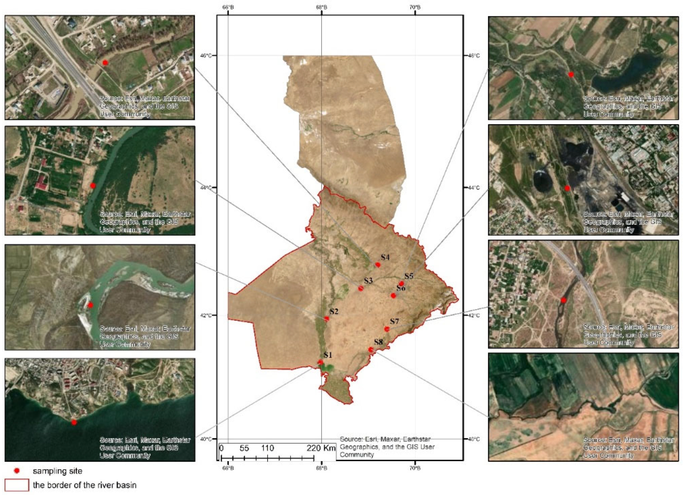

| № | Sampling Location | Geocoordinates | Location Description | Anthropogenic Activities (According to S.P. Gorshkov Classification) | Water Temperature (°C) | Elevation | Sampling Date |
|---|---|---|---|---|---|---|---|
| 1 | S1 Shardara Reservoir | 41°14’44.70”N, 67°58’50.41”E | 100m southeast of Shardara city | Water Management: Reservoir (Shardara Reservoir) Recreation: Rest areas (“GOLDEN BEACH RESORT”) |
18°C | 255m | 01.08.2024 |
| 2 | S2 Syr Darya River | 41°56’20.82”N, 68°6’20.28”E | 500m east of Sütkent village | Agriculture: Livestock, Haymaking (“Bolashak” farm) Crop production: Irrigated agriculture (57,800 hectares) Grazing (600,000–700,000 hectares) |
19°C | 213m | 01.08.2024 |
| 3 | S3 Arys River | 42°26’25”N, 68°50’38”E | 700m east of Arys city | Urban Industrial: Food industry (meat, dairy, flour products) Mining Industry: Non-metallic minerals (bentonite, limestone) Agriculture: Livestock, Haymaking (“Argynbek” farm) Crop production: (“Mubarak Agro” farm) Grazing (426,643 hectares) |
18°C | 224m | 01.08.2024 |
| 4 | S4 Bogen River | 42°47’45”N, 69°12’20”E | 58m south of Ekpindi village | Agriculture: Livestock, Haymaking (“Zher-Nur” cooperative) Crop production: Irrigated agriculture (93,000 hectares) Grazing (600,000–700,000 hectares) |
18°C | 256m | 02.08.2024 |
| 5 | S5 Aksu River | 42°29’27”N, 69°43’29”E | 710m southeast of Karabulak village | Agriculture: Livestock, Haymaking (“Karabulak” farm) Crop production: (“Aisha” farm) Grazing (8234 hectares) |
19°C | 485m | 03.08.2024 |
| 6 | S6 Badam River | 42°18’38”N, 69°32’14”E | 100m south of “Yuzhpolimetal” JSC | Urban Industrial: Food industry (vegetable oils, flour, dairy, pasta products) Light industry: Textile, production companies Construction industry: New ceramic tile factory Metal processing industry: Metallurgical plant |
17°C | 463m | 03.08.2024 |
| 7 | S7 Keles River | 41°47’37”N, 69°25’16”E | 5.9 km north of Kazygurt village | Urban Industrial: Food industry (instant noodles, natural juice, dry milk) Construction industry: “Reinforced concrete products” factory Agriculture: Livestock, Haymaking (“Saydusman Ata” farm) Crop production: (“Nur-Aidar” farm) Grazing (133,460 hectares) |
17°C | 603m | 04.08.2024 |
| 8 | S8 Kurkeles River | 41°29’41”N, 69°07’42”E | 300m southwest of Saryagash city | Urban Industrial: Food industry (mineral water, wine, flour products) Light industry: Cotton fiber production Recreation: Resorts Agriculture: Livestock, Haymaking (“Kuanish Myktybaev” farm) Crop production: (“Kamiljan” farm) Grazing (294,579 hectares) |
19°C | 393m | 05.08.2024 |
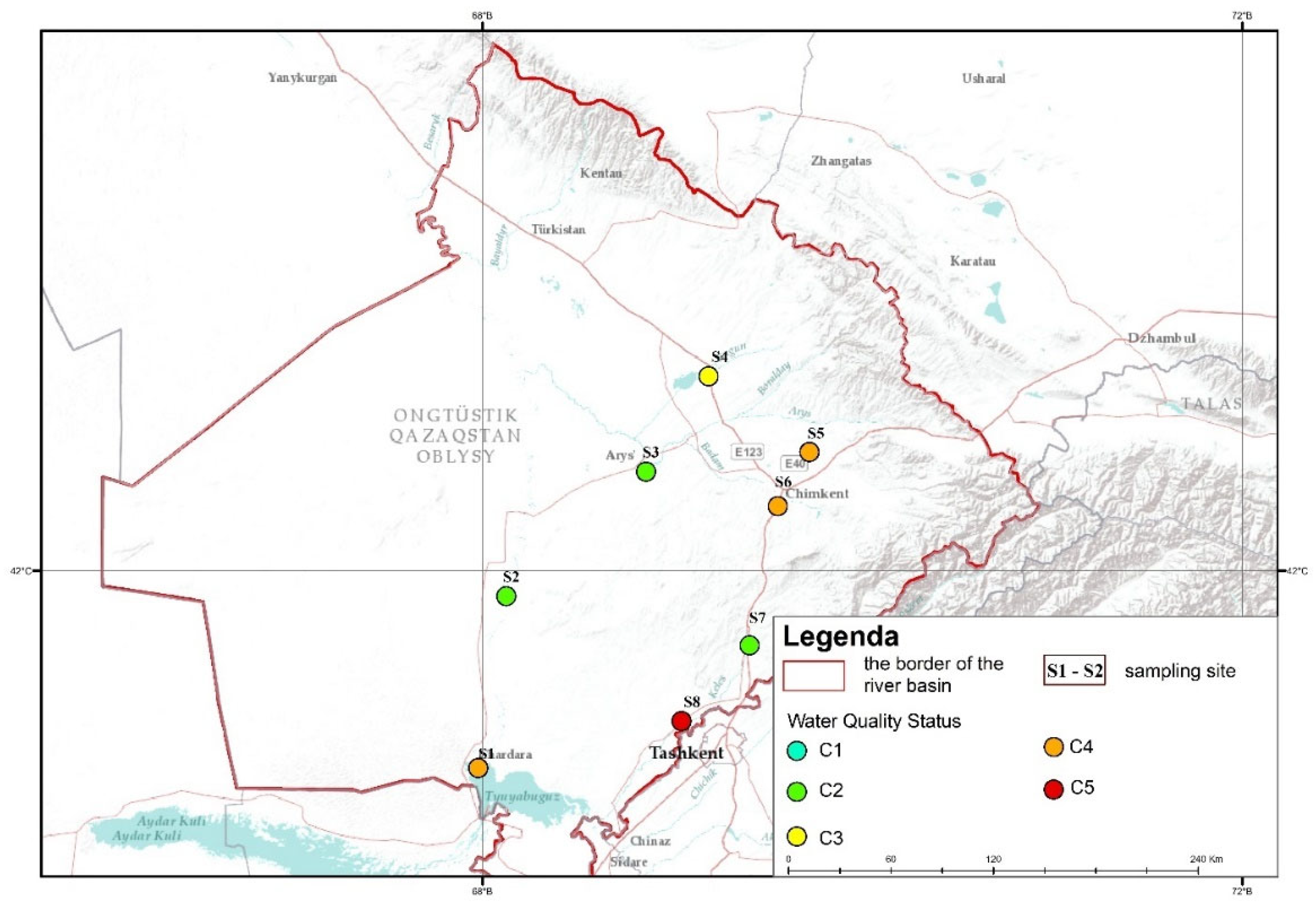
| Water Quality Status | Class | pH | Hardness (mg/l) | Lyness (mg/l) | BOD (mg/l) | TDS (mg/l) |
|---|---|---|---|---|---|---|
| Best water quality | C1 | 6.5–8.5 | 50–75 | <5 | <3 | <1000 |
| Water suitable for all types of use; simple purification required for domestic and drinking water supply | C2 | 6.0–6.5 and 8.5–9.0 | 100–150 | 5–10 | 3–6 | 1000–1500 |
| Suitable for recreational use (swimming and other leisure activities), irrigation, industry, fish farming (carp species); normal treatment required for domestic and drinking water supply | C3 | 5.0–6.0 and 9.0–9.5 | 150–250 | 10–50 | 6–10 | 1500–2000 |
| Suitable for irrigation and industry; deep water treatment methods required for domestic drinking water supply | C4 | <5.0 and >9.5 | >250 | 50–100 | 10–20 | >2000 |
| Actual concentration exceeds Class 5 norm | C5 | <5.0 and >9.5 | >500 | >100 | >20 | >3000 |
| Parameters | X ± S x | lim | P | σ | CV, % |
|---|---|---|---|---|---|
| Total hardness, mg*eq/L | 7,00±0,89 | 10,64-1,92 | 8,72 | 3,08 | 43,94 |
| Hydrogen index of water (pH) | 8,13±0,04 | 8,39-7,94 | 0,45 | 0,14 | 1,71 |
| Total dissolved solids, mg/L | 949,75±110,39 | 1614-512 | 1102 | 382,40 | 40,26 |
| Aluminum (Al), mg/L | 5,39±2,15 | 22,38-0,00 | 22,38 | 7,43 | 137,99 |
| Calcium (Ca), mg/L | 108,30±11,85 | 161-25 | 136 | 41,06 | 37,91 |
| Magnesium (Mg), mg/L | 55,73±4,82 | 78-27 | 51 | 16,68 | 29,94 |
| Potassium (K), mg/L | 6,15±0,65 | 9,99-3,40 | 6,59 | 2,24 | 36,45 |
| Sodium (Na), mg/L | 101,80±15,45 | 180,05-38,72 | 141,33 | 53,51 | 52,57 |
| Sulfates (SO₄²⁻), mg/L | 337,18±64,78 | 639-92,2 | 546,8 | 224,40 | 66,55 |
| Electrical conductivity, µS/cm | 1107,75±133,94 | 1714-555,00 | 1 159 | 463,97 | 41,88 |
| 1.X ± Sx – mean ± standard error; 2.lim – range of limits; 3.p – critical difference; 4.σ – standard deviation; 5.CV % – coefficient of variation. | |||||
| Sampling Site | OPI Value | Water Quality Status | Class |
|---|---|---|---|
| S1 | 3.1 | Significant Pollution | 4 |
| S2 | 0.56 | Satisfactory | 2 |
| S3 | 0.43 | Satisfactory | 2 |
| S4 | 1.27 | Moderate Pollution | 3 |
| S5 | 2.38 | Significant Pollution | 4 |
| S6 | 3.68 | Significant Pollution | 4 |
| S7 | 0.73 | Satisfactory | 2 |
| S8 | 12.14 | Highly Polluted | 6 |
| Indicator | MAC (mg/L) | S1 | S2 | S3 | S4 | S5 | S6 | S7 | S8 |
|---|---|---|---|---|---|---|---|---|---|
| Total Hardness, mg*eq/L | 7 | 1 | 1 | 0 | 0 | 0 | 1 | 1 | 0 |
| pH | (6.5, 8.5) | 0.934 | 0.944 | 0.955 | 0.987 | 0.965 | 0.955 | 0.964 | 0.944 |
| Dry Residue, mg/L | 1000 | 1 | 1 | 1 | 1 | 1 | 1 | 2 | 1 |
| Aluminum (Al), mg/L | 0.5 | 13 | 0 | 0 | 5 | 11 | 12 | 0 | 45 |
| Arsenic (As), mg/L | 0.1 | - | - | - | - | - | - | - | - |
| Boron (B), mg/L | 0.5 | - | - | - | - | - | - | - | - |
| Calcium (Ca), mg/L | 200 | 0.7 | 0.5 | 0.5 | 0.1 | 0.5 | 0.6 | 0.6 | 0.8 |
| Cadmium (Cd), mg/L | 0.005 | 0 | 0 | - | - | 0 | - | - | - |
| Cobalt (Co), mg/L | 0.1 | 0 | 0 | - | 0 | 0 | - | - | - |
| Chromium (Cr), mg/L | 0.05 | - | - | - | 0.1 | - | - | - | - |
| Titanium (Ti), mg/L | - | - | - | - | - | - | - | - | - |
| Iron (Fe), mg/L | 0.3 | - | - | - | 8 | - | - | - | 43 |
| Lead (Pb), mg/L | 0.01 | - | - | - | - | - | - | - | - |
| Copper (Cu), mg/L | 1 | - | - | - | - | - | - | - | - |
| Magnesium (Mg), mg/L | 50 | 1.44 | 1.06 | 0.9 | 0.54 | 0.96 | 1.08 | 1.56 | 1.38 |
| Potassium (K), mg/L | 10 | 0.9 | 0.5 | 0.3 | 0.6 | 0.5 | 0.6 | 0.4 | 1 |
| Manganese (Mn), mg/L | 0.1 | - | - | - | - | - | - | - | - |
| Sodium (Na), mg/L | 200 | 0.7 | 0.5 | 0.3 | 0.2 | 0.3 | 0.3 | 0.9 | 0.8 |
| Nickel (Ni), mg/L | 0.02 | - | - | - | - | - | - | - | - |
| Zinc (Zn), mg/L | 5 | - | - | - | - | - | - | - | - |
| Sulfates (SO₄²⁻), mg/L | 500 | 1 | 1 | 0 | 0 | 0 | 0 | 1 | 0 |
| Phenol (C₆H₅OH), mg/L | 0.001 | - | - | - | - | - | - | - | - |
| Electrical Conductivity, µS/cm | 1000 | 1.6 | 1.2 | 0.8 | 0.6 | 0.6 | 0.8 | 1.7 | 1.5 |
| Total Salinity, mg/L | 1000 | 1 | 1 | 0 | 0 | 0 | 1 | 1 | 0 |
| Sampling Site | HPI Value | Interpretation |
|---|---|---|
| S1 | 19.19 | Safe and clean water (low pollution level). Water quality meets ecological standards. |
| S2 | 20.00 | Safe and clean water (low pollution level). No risk to ecosystems or human health. |
| S3 | 2.00 | Safe and clean water (very low pollution level). Water quality is very good. |
| S4 | 120.38 | Highly polluted water. Heavy metal concentrations exceed the norm, posing a risk to ecosystems and human health. |
| S5 | 19.09 | Safe and clean water (low pollution level). Meets ecological and sanitary standards. |
| S6 | - | No data (sample not taken or measurement results unavailable). |
| S7 | - | No data (sample not taken or measurement results unavailable). |
| S8 | 4253.33 | Extremely polluted water. Heavy metal concentrations are very high, posing significant risks to water ecosystems and human health. This water should be prohibited for use. |
| Pollutant | Occurs in LULC (Land Use Types) | Natural Sources | Anthropogenic Sources | Ecological Impacts | Technical Solutions |
|---|---|---|---|---|---|
| Al | S4, S8 | Industrial areas, agriculture, construction, open land | Soil erosion, rock weathering, forest fires | Industrial waste, fertilizers, pesticides, water treatment reagents | Degradation of water ecosystems, inhibits crop growth |
| Cd | S1, S2, S5 | Croplands, rural areas | Natural dust, volcanic activity | Pesticides, batteries, industrial waste | Bioaccumulation in aquatic organisms, disrupts food chain |
| Ca | S4 | Farmland, grazing areas | Limestone, volcanic rocks, mineral solubility | Construction waste, livestock farming | Soil structure degradation, fertility decline |
| Fe | S4 | Bogen River, agricultural areas | Magmatic rocks, organic waste | Construction waste, runoff | Disruption of water ecosystems, damage to fish and plants |
| Mg | S8 | Farmland, grazing areas | Magmatic rocks, limestone | Livestock feed, fertilizers | Mineralization of water ecosystems, habitat changes |
| Na | S1-S8 | Suburban areas, agriculture | Silicate minerals, sea salt | Road salt, household softeners | Soil and groundwater salinization |
| Aquatic Plant | Heavy Metal Accumulation Potential | Accumulated Metals |
|---|---|---|
| Populus spp. (Poplar) | High | Pb, Cd, Cu, Zn |
| Tamarix spp. (Tamarisk) | High | As, Pb, Zn, Cd |
| Phragmites australis (Reed) | High | Fe, Cu, Cd, Pb, Zn |
| Carex spp. (Sedge) | Medium | Cu, Zn, Pb |
| Medicago sativa (Alfalfa) | Medium | Pb, Cd, Zn |
| Lupinus spp. (Lupine) | High | Pb, Cd, Ni, Zn |
| Typha latifolia (Bulrush) | High | Pb, Zn, Mn, Ni, Fe, Cu |
| Salix spp. (Willow) | Medium | Pb, Cd, Zn |
| Mechanism in Aquatic Plants | Pollutants | Description | Site of Action | Plant Examples |
|---|---|---|---|---|
| Phytoextraction / Phytoaccumulation | Organic / Inorganic Pollutants | Absorption through roots and transport to aerial parts. Absorption from water and air. | Leaves | Juncus repens, Pistia stratiotes |
| Rhizofiltration / Phytofiltration | Organic / Inorganic, Heavy Metals | Removal through adsorption/absorption from polluted water. | Stems / Roots | Lemna minor, Hydrocharis morsus, Eichhornia crassipes |
| Phytostabilization / Phytoaccumulation / Phytosequestration | Heavy Metals, Cd and Zn | High bioconcentration and transport coefficients. | Roots | E. crassipes, Typha angustifolia |
| Phytodegradation / Rhizodegradation | Organic / Inorganic | Breakdown through microbiological degradation or plant metabolism. | Rhizosphere for pollutant degradation | Typha angustifolia, Myriophyllum aquaticum |
| Phytovolatilization | Organic Compounds | Transformation and release of pollutants to the atmosphere. | Atmospheric release | Phragmites australis, Typha minima |
Disclaimer/Publisher’s Note: The statements, opinions and data contained in all publications are solely those of the individual author(s) and contributor(s) and not of MDPI and/or the editor(s). MDPI and/or the editor(s) disclaim responsibility for any injury to people or property resulting from any ideas, methods, instructions or products referred to in the content. |
© 2025 by the authors. Licensee MDPI, Basel, Switzerland. This article is an open access article distributed under the terms and conditions of the Creative Commons Attribution (CC BY) license (https://creativecommons.org/licenses/by/4.0/).


