
Submitted:
14 December 2024
Posted:
16 December 2024
You are already at the latest version
Abstract
Weeds remain as one of the major limiting factors affecting agricultural production and crop productivity and cause significant yield loss globally. Alternate to traditional control of weeds with broadcast application of herbicides, spot spraying of weeds is commensurate with patchy spatial distribution of weeds. But the displacement of spray caused by wind and rotor wash remains a major concern, which can lead to inefficient coverage and unintended environmental loading. To mitigate this issue, drop nozzles have been developed to direct the spray closer to the target, thereby reducing drift and enhancing spray efficacy. A remotely piloted aerial application system (RPAAS) was outfitted with a 60 cm drop nozzle comprised of a straight stream and a 30° full cone nozzle to increase spray accuracy by reducing the effect of wind on spray displacement. Wind speed averaged 5.63 ± 0.40 m/s and varied from 2.23 to 8.94 m/s. A fluorescent spray solution was applied on 13 Kromekote cards placed in a grid configuration. The center of deposition for each of the spray applications was determined using Python software. Spray displacement was calculated as the distance between the center target site and the center of deposition for each of the spray applications. Regardless of nozzle angle, the drop nozzle produced significantly less spray displacement compared to the no drop nozzle, which should increase herbicide efficacy of targeted applications.
Keywords:
precision agriculture
; drop nozzle
; spray displacement
; straight stream nozzle
; nozzle angle
1. Introduction
Weeds are one of the major limiting factors to the production of agricultural crops and cause significant yield loss in crop farming systems throughout the world. It is estimated that weeds in corn and soybean alone would reduce yield by 50%, costing growers $43 billion in economic loss annually in the United States and Canada according to a study conducted over a seven-year period [1]. When a pre-emergence herbicide was used, surviving weeds began to reduce corn yields after about 6 weeks with grasses having greater effect than broadleaf weeds [2]. Early germinating weeds reduce yield more than weeds which emerge later in the growing season [3]. Most importantly, recent events due to climate change has precipitated increased concentration of CO2 in the atmosphere which can influence the efficacy of herbicides and weed management. The C3 weeds would be able to develop resistance to glyphosate, a non-selective, post-emergent widely used herbicide, more easily than C4 weeds under increased concentration of CO2 [4,5,6].
The cost for weed control in North American farmlands remain high and controlling weeds efficiently is, therefore, imperative for reducing farmers’ overhead costs and to increase farm productivity [7]. The conventional approach for controlling weeds in production agriculture has relied on broadcast applications of herbicides across the entire field. This approach has brought in its wake environmental concerns and concomitant resurgence of resistant weeds. Spot spraying of weeds as an alternative method is commensurate with the spatial distribution of weeds since they often occur in patches within crop fields [8,9]. Using geostatistics, Johnson et al. [8] reported that inherent variability of seed dispersal, germination, seed and seedling mortality events primarily contribute to the patchy distribution of weed populations. Besides weeds, arthropod pest outbreaks in production in agriculture often occur as clumped or as contagious, skewed spatial pattern. For instance, cabbage aphids in canola fields, and Asian psyllids in citrus orchards occur as highest population densities along field edges [10,11,12]. Aphids on soybean and two-spotted spider mites on cowpea when exposed to abiotic stress, such as drought or nutrient deficiencies tend to be more susceptible [13,14,15]. Thus, as pests occur as spatially aggregated and heterogeneous cohorts, precision technology can offer opportunities for controlling these organisms without unduly affecting the environment [16].
The integration of drone technology or remotely piloted aerial application systems (RPAASs) into farming practices is a significant advancement in crop management, particularly in the application of pesticides and herbicides. One of the primary challenges in this domain is the displacement of spray caused by wind and rotor wash, which can lead to inefficient coverage and deleterious effects on environment. To mitigate this issue, the drop nozzles have been developed which extend below the main body of the drone, enabling the delivery of chemicals closer to the crop canopy and reducing the distance the spray must travel before reaching the target. This design minimizes the likelihood of spray drift, as it decreases exposure to wind shear and enables more direct spray application. Moreover, drop nozzles provide improved canopy penetration, ensuring better coverage of weeds and pests, particularly in dense or tall cropping systems. The RPAAS platforms utilize advanced sensors and algorithms for on-line weed detection using digital image analysis, computer-based decision making and GPS-controlled patch spraying. This helps identify and treat specific areas infested with weeds, minimizing the use of chemicals and promoting sustainable agricultural practices.
Objectives of this study were to evaluate the role of drop nozzles for increasing spray accuracy by reducing the effect of wind speed on spray displacement. Specfically, we wanted to determine the effect of drop nozzles on spray displacement vis-à-vis wind speed which is a major impediment to targeted applications.
2. Materials and Methods
This study was conducted in an unpaved area surfaced with gravel in Burleson County, near College Station, TX (30° 40´ N, 96° 18´ W). The targeted spray location comprised of 13 wooden blocks established in a grid where the number 7 was the center target card which served as the cynosure of spray deposition (Fig. 1). These wooden blocks (38 x 89 x 76 mm) were arranged with a 0.31 m spacing between each other. A paper clip was attached to each of the blocks with a sheet metal screw. An 89 x 89 mm Kromekote card (CTI Paper USA, Neenah, WI, USA) was placed into each paper clip. The RPAAS used was a six rotor, sixteen-liter Precision Vision 35X (PV35X, Leading Edge Aerial Technologies, New Smyrna Beach, FL) (Fig. 2). It has a custom single spot-spray nozzle mounted directly underneath the fuselage (Fig. 3). The RPAAS was equipped with an RTK guidance system (Herelink 2, Hex Technology, Austin, TX, USA) while spraying to provide centimeter level accuracy to hit the center target card (card 7) on the grid. Four nozzle configurations; 1) 30° with a 60 cm drop (30D), 2) 30° with no drop (30ND), 3) straight stream with 60 cm drop (SSD), and 4) straight stream with no drop (SSND) were used. The drop tube was a braided steel hose (BrassCraft, Novi, MI, USA) with washers sitting on top of the nozzle to reduce swing due to wind (Fig. 4). The spray solution comprised of water plus Rhodamine dye mixed at 20 ml/L was sprayed on Kromekote cards as shown in Figure 1. The treatments used in this study were described in Table 1.
2.1. Determination of Spray Displacement
Once the RPAAS had the coordinates of the center card, it was moved to the takeoff location. For all treatments the RPAAS hovered at 1.52 m over the target area. For the no drop nozzle treatments, the nozzle height was equal to the RPAAS height. For the drop nozzle treatments, the nozzle height was 0.92 m over the target area. The pump pressure was set at 345 Kpa (50 psi). The RPAAS was programmed to hover over the target area for 5 seconds to stabilize its x, y and z (latitude, longitude, and height) position and the nozzle prior to the spray application. The spray was released for 1 second which provided a dose of 30 ml (1 oz). The Kromekote cards were left for 3-5 minutes to dry on the wooden blocks before being moved to a table before transporting to the laboratory for processing. Wind speed, wind direction and temperature were measured during each spray applications (Table 2 and Table 3). The weather conditions during the study were variable with wind speed, being the major determinant that influenced spray displacement. For the 0° angle drop nozzle treatment, the wind speed varied from 5 to 9 m/s, while for 30° angle drop nozzle treatment, the wind speed varied from 2 to 7 m/s. This indicates that the wind speed during the test was not evenly distributed for the 0° and 30° angle tests and thus, it remains as a limiting factor in this study.
A coordinate point was assigned to every Kromekote card on the grid. The Python software [17] was used to generate a heat map showing the % area coverage for each treatment. Two libraries, NumPy and pandas, were used to analyze the data and convert it into data that could be used by the graphic design library matplotlib. Pandas performs data preparation in the form of tables and spreadsheets, while NumPy is used numerical computation of the data. The program used a sigmoid interpolation to better represent the % area coverage. The centroid was calculated using Python software to identify the center of spray deposition (Figure 5).
2.2. Determination of Spray Droplet Characteristics
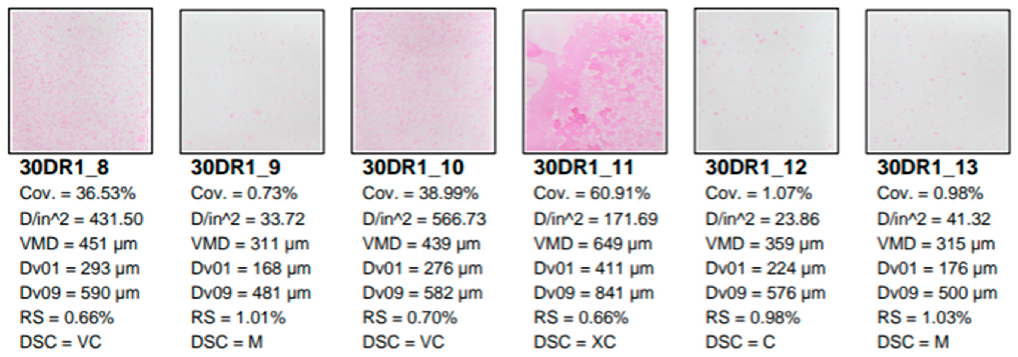
The Kromekote cards were analyzed using the AccuStain software (University of Illinois at Urbana-Champaign, Urbana-Champaign, IL, USA). A representative sample of these analyzed cards is shown below (Figure 6). The cards were placed in order of top to bottom of the grid (Figure 1). Spray droplet spectra measured were Dv0.1, Dv0.5, Dv0.9, percent area coverage and relative span (RS). Dv0.1 is the droplet diameter (µm) where 10% of the spray volume is contained in droplets smaller than this value. Similarly, Dv0.5 and Dv0.9 are droplet diameters where 50 and 90% of the spray volumes are contained in droplets smaller than these values, respectively. Dv0.5 is commonly known as the volume median diameter (VMD). RS is a dimensionless parameter and measures the width of the droplet spectra around Dv0.5, describing the uniformity of the drop size distribution and is calculated as:
(Dv0.9 - Dv0.1)/ Dv0.5
The American Society of Agricultural and Biological Engineering has developed the ASABE S572.3 Droplet Size Classification, a standard to measure and interpret spray quality tips for aerial application spray nozzles [18]. The VMD of the spray droplet sizes that were released from the spray tips in this study were comprised of fine (106-235 µm), medium (236-340 µm), coarse (341-403 µm), very coarse (404-502 µm) and extra coarse (503-760 µm) spray droplet spectra.
Figure 6.
Representative sample of Kromekote cards with rhodamine dye deposits describing droplet spectra from a field study analyzed with AccuStain software.
Figure 6.
Representative sample of Kromekote cards with rhodamine dye deposits describing droplet spectra from a field study analyzed with AccuStain software.
All statistical analysis of the data were conducted using the JMP® software [19]. The assumption of homogeneity of variance is a prerequisite while conducting ANOVA and to obtain reliable results [20]. To test the equality of variance of the data, the drop and no drop nozzle data were pooled and were then sorted by 0°and 30° angles. The Levene’s test was performed for each of the spray droplet spectra from 0°and 30° angles to test the null hypothesis that the variances were equal (Table 3). The results of the analysis indicated that although some of the droplet parameter data did represent unequal variance, the majority of the data (58%) were homoscedastic. Therefore, the analysis of variance of the spray droplet data was conducted without transformation. The analysis of means, (ANOM) which is an alternative to one-way analysis of variance (ANOVA) for a fixed effects model was used to compare the slopes between drop and no drop nozzle and that between nozzles set at 0° and 30° [21]. Unlike ANOVA, which simply determines whether there is a statistically significant difference between treatment means, ANOM identifies the means that are significantly different from the overall mean.
3. Results
3.1. Spray Droplet Spectra
The spray droplet characteristics determined for the treatments used in this
study is presented in Table 4. Regardless of nozzle angle, there was no significant difference in % percent area coverage or droplet density between drop and no drop nozzle. The Dv0.1 spray droplets differed significantly between drop and no drop nozzles for the 30° nozzle but not for the 0° nozzle. The no drop nozzle produced larger Dv0.1 droplets than the drop nozzle. This suggests that the drop nozzle being closer to the target most of smaller droplets reached the target instead being blown away by the wind. For VMD, the trend was like that for the Dv0.1 spray droplets. The Dv0.9 droplets were not significantly different between drop and no drop nozzles, regardless of nozzle angle. However, the RS which measures the width of the droplet spectra around Dv0.5 droplets, varied significantly between drop and no drop nozzles for both 0° and 30° nozzles. The no drop nozzles had a narrower RS compared to the drop nozzles. A plausible explanation for this effect may be that the smaller, more driftable fractions of the spray was not able to deposit on the targets due to spray displacement from the wind. This would reduce the RS which is based on the difference between Dv0.9 and Dv0.1 divided by Dv0.5. When smaller droplet fraction is blown away from the target, the Dv0.1 value increases, thus making the difference between Dv0.9 and Dv0.1 smaller, which reduces the RS.
3.2. Spray Displacement Analysis
Figure 7 shows that the spray displacement for the drop nozzle was smaller compared to the no drop nozzle oriented at 0° (F=5.81; P=0.04; df=1, 8). Figure 8 shows that a similar trend was evident when the nozzle was oriented at 30° (F=6.55; P=0.03; df=1,8).
When the data were combined by nozzle angle (0° and 30°) and analyzed to determine the effect of drop vs no drop nozzle, the treatments were significantly different (F=12.84; P=0.0021; df=1, 18). The drop nozzle produced significantly smaller displacement than the no drop nozzle (0.18341 m vs 0.32215 m) and accounted for 76% reduction in displacement.
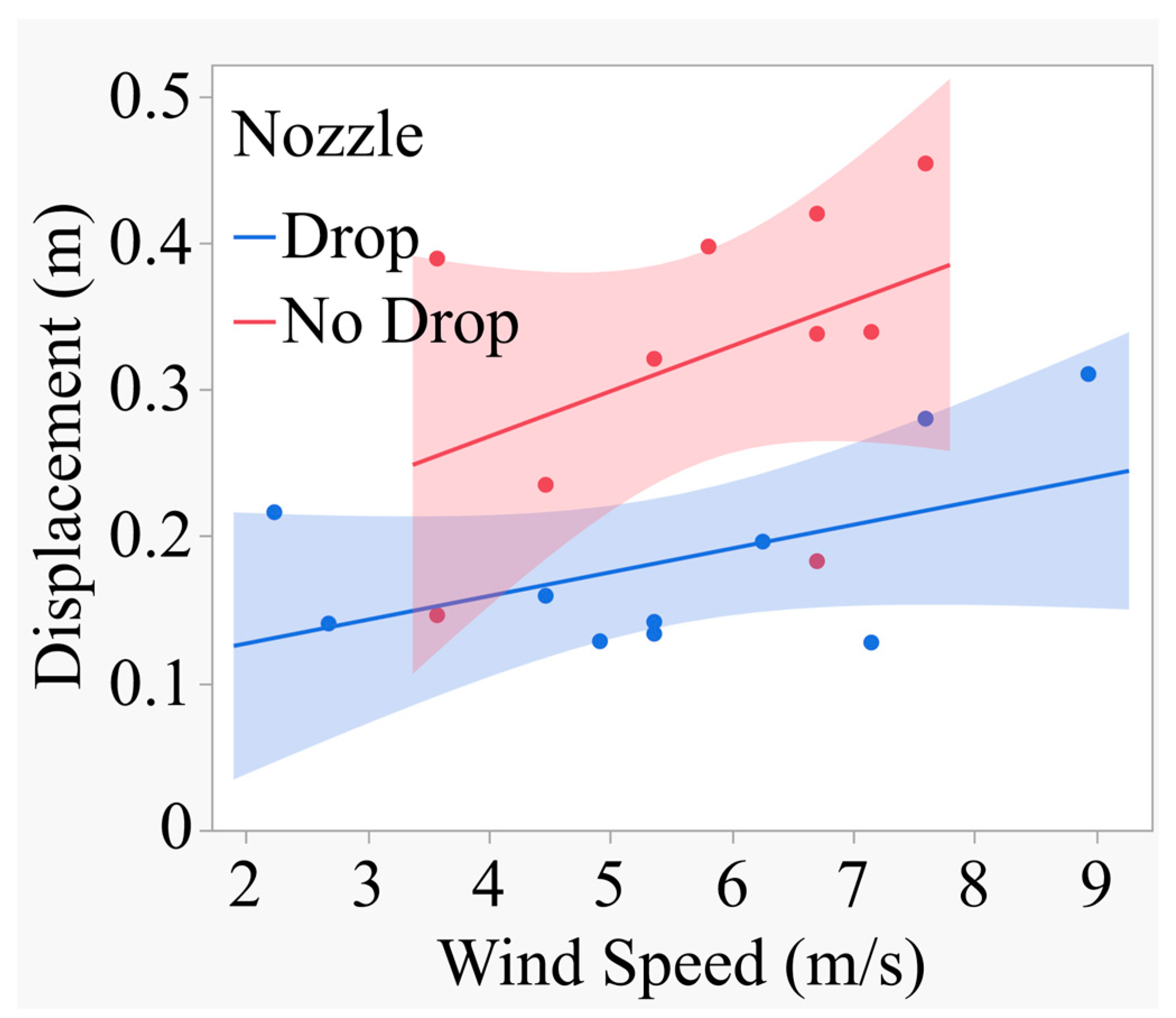
Figure 10.
shows the relationship between spray displacement and wind speed for the drop nozzle compared to no drop nozzle.
Figure 10.
shows the relationship between spray displacement and wind speed for the drop nozzle compared to no drop nozzle.
3.3. Comparisons with Overall Average Decision Chart
Figure 11 shows that there was no significant difference in slopes between drop and no drop nozzles. Both slopes are within the upper and lower confidence limits, one being above the UDL (No Drop) and the other being below the LDL (Drop). The regression of displacement on wind speed was upward and linear for both nozzles (Fig. 10). The slope is at the rate of b units of Y per unit of X, where b is the sample regression coefficient. The following equations explained the relationship between spray displacement and wind speed for both drop and no drop nozzles.
Y=0.09451 + 0.016171*X; R2=0.26 (Drop Nozzle)
Y=0.1446 + 0.03079*X; R2=0.19 (No Drop Nozzle)
These equations accounted for only 26 and 19% of the variations in the model. The rate of increase in displacement for the drop nozzle was 0.01617 unit for each unit increase in wind speed. Similarly, the rate of increase in displacement for the no drop nozzle was 0.03079 unit for each unit increase in wind speed. The slope for the no drop nozzle was slightly higher numerically than that for the drop nozzle and statistical differences between them could not demonstrated. However, the drop nozzle produced significantly smaller spray displacement (t=-3.62; P=0.0023) compared to the no drop nozzle (0.18341m vs 0.32215 m). The data thus indicate that the drop nozzle produced about 76% lower spray displacement than the no drop nozzle. The test for the homogeneity of the regression indicated that there was no significant difference between the two slopes. This suggests that the rate of spray displacement relative to wind speed was comparable between the drop and no drop nozzle and that the wind speed acted squarely for both nozzles.
The following equation for the 0 and 30 angle nozzles described the relationship:
Y=-0.1728 + 0.06644*X R2= 0.46 for the 0° nozzle
Y = 0.2145 + 0.004023*X R2 = 0 for the 30° nozzle.
The slope coefficient for the 0° nozzle was significantly different from zero (F=6.86; P=0.0307; df=1, 8) and suggests that displacement increased by 0.06644 m unit for every unit increase in wind speed. The slope coefficient for the 30° angle nozzle was near zero and that it did not vary significantly from zero (F=0.03; P=0.8633; df=1, 8). It is apparent from the regression equation that displacement increased linearly with wind speed for the 0° nozzle. For the 30° nozzle, the regression coefficient was a flat line which indicated that the displacement did not increase with wind speed. One of the limitations of the study is that the wind speed during the test did not encompass equally for both the nozzles. As wind speed is beyond our control, it is important that more tests should be conducted over a range of wind speed, replicated over time and space in order to obtain a better perspective on the relationship between displacement and wind speed for these nozzle angles.
4. Discussion
Zhou et al. [22] reported that the farmers in the southern United States control glyphosate resistant weeds on cotton using labor intensive methods including hand hoeing, hand spraying, spot spraying and wick applicator. Recently, Unan et al. [23] reported that using a backpack sprayer, spot spraying of clethodim herbicide applied at the labeled rate (150 g ai ha−1) in a flooded rice field successfully controlled weedy rice and grasses without dispersion of the chemical. Herbicide dispersion is a common problem in flooded rice fields, which can damage adjacent crops and have negative impacts on the non-target species’ composition, biodiversity, and reproduction. In rice ecosystem, during the dispersion process, herbicides can spread, become immersed, and then rise to the surface where they can float or continue to float without the initial submersion [23]. Allmendinger et al. [24] reported that besides herbicide reduction, the spot spraying reduced environmental risks associated with herbicide, including herbicide leaching into the ground water, herbicide resistance development in weeds, and herbicide residues in the food chain and drift.
In this study, a significant reduction in spray displacement was observed for the drop nozzle, regardless of the nozzle angle used. This indicates that adding a 0.6 m drop tube to a spot spraying RPAAS can increase accuracy of deposition at the wind speed that occurred during the study. Wind speed averaged 5.63 ± 0.40 m/s and varied from 2.23 to 8.94 m/s. More studies on the efficacy of drop nozzles in reducing spray displacement are warranted at various wind speeds to better understand this technology. There is little research data on the use of RPAAS platforms retrofitted with drop nozzles vis-à-vis spray displacement under field conditions where the vagaries of weather predominate. Allmendinger et al. [24] reported on commercially available spot spraying systems comprised of sensors and classifiers for weed detection and decision algorithms to decide whether weed control is needed. A survey conducted on farmers in the southern United States indicated that resistant weed control on cotton were performed using labor intensive techniques and that no education programs on better weed management technique was developed to help the farmers. A crucial next step in researching spot spraying with RPAAS is to investigate the effects of rotor wash on spray droplets to determine whether they reach the intended target area. The characteristics of rotor wash can vary greatly between each RPASS due to factory-installed configurations of these platforms. While several studies have examined the impact of rotor wash on a multi-rotor RPAAS platforms [25,26,27,28], few data exist for spray drones configured for spot spraying. The down-wash air flow generated by rotor wings can significantly influence deposition, penetration, distribution and swath width of the RPAAS platforms. The air flow could also help penetration of the spray droplets into the lower canopy [25,26,27]. Richarson et al. [29] reported that for conventional aerial spraying, deposition is measured along the sampling line perpendicular to the direction of the flight, while for spot spraying, the deposition pattern is two-dimensional. These data warrants further investigation.
5. Conclusions
This study has shown that a drop nozzle with a straight stream or 30° cone nozzle can minimize spray displacement and facilitate more precise applications of herbicides for weed control. Thus, this technique of using drop nozzle for the control of resistant weeds can help minimize off-target movement of hazardous chemicals and mitigate spray drift. The drop nozzle system used in this study was improvised and outfitted to the RPAAS platform. The potential to increase farm productivity by reducing input costs make this method of chemical application an alternative to current spot spraying methods. This study has shown that wind speed was twice as much higher when the 0° angle nozzle was tested compared to the 30° angle nozzle test. Thus, additional research evaluating the accuracy and efficacy of herbicide applications under various meteorological conditions should help understand this spot spraying technology for resistant weed control.
Author Contributions
Conceptualization, D.M. and S.N.; methodology, D.M..; software, R.G.; validation, R.G., Z.H.; formal analysis, R.G.; resources, D.M.; M. A. L., writing—original draft preparation, R.G.; writing—review and editing, R.G., D.M., Z.H., S.N.; M. A. L., visualization, R.G.; All authors have read and agreed to the published version of the manuscript.
Funding
This research received no external funding.
Data Availability Statement
We encourage all authors of articles published in MDPI journals to share their research data. In this section, please provide details regarding where data supporting reported results can be found, including links to publicly archived datasets analyzed or generated during the study. Where no new data were created, or where data is unavailable due to privacy or ethical restrictions, a statement is still required. Suggested Data Availability Statements are available in section “MDPI Research Data Policies” at https://www.mdpi.com/ethics.
Acknowledgments
In this section, you can acknowledge any support given which is not covered by the author contribution or funding sections. This may include administrative and technical support, or donations in kind (e.g., materials used for experiments).
Conflicts of Interest
The authors declare no conflicts of interest. Authors must identify and declare any personal circumstances or interest that may be perceived as inappropriately influencing the representation or interpretation of reported research results. Any role of the funders in the design of the study; in the collection, analyses or interpretation of data; in the writing of the manuscript; or in the decision to publish the results must be declared in this section. If there is no role, please state “The funders had no role in the design of the study; in the collection, analyses, or interpretation of data; in the writing of the manuscript; or in the decision to publish the results”.
References
- Soltani, N.; Dille, J.A.; Burke, I.C.; Everman, W.J.; VanGessel, M.J.; Davis, V.M.; Sikkema, P.H. Potential corn yield losses from weeds in North America. Weed Technol. 2016, 30, 979–984. [Google Scholar] [CrossRef]
- James, T.; Rahman, A.; Mellsop, J. Weed competition in maize crop under different timings for postemergence weed control. New Zeal. Plant Protect. 2000, 53, 269–272. [Google Scholar] [CrossRef]
- Sardana, V.; Mahajan, G.; Jabran, K.; Chauhan, B.S. Role of competition in managing weeds: An introduction to the special issue. Crop Protect. 2017, 95, 1–7. [Google Scholar] [CrossRef]
- Fernando, N.; Manalil, S.; Florentine, S.K.; Chauhan, B.S.; Seneweera, S. Glyphosate resistance of C3 and C4 weeds under rising atmospheric CO2. Front. Plant Sci. 2016, 7, 910. [Google Scholar] [CrossRef]
- Kaur, R.; Kumar, S.; Ali, S.; Kumar, S.; Ezing, U.; Bana, R.; Meena, S.; Dass, A.; Singh, T. Impacts of climate change on crop-weed dynamics: Challenges and strategies for weed management in a changing climate. Open J. Environ. Biol. 2024, 9, 015–021. [Google Scholar] [CrossRef]
- Amare, T. Review on impact of climate change on weed and their management. Amer. J. Biol. Environ. Statis. 2016, 2, 21–27. [Google Scholar] [CrossRef]
- Baldwin, F.L. Transgenic crops: a view from the US Extension Service. Pest Manage Sci. 2000, 56, 584–585. [Google Scholar] [CrossRef]
- Johnson, G.A.; Mortensen, D.A.; Gotway, C.A. Spatial and temporal analysis of weed seedling populations using geostatistics. Weed Sci. 1996, 44, 704–710. [Google Scholar] [CrossRef]
- Nobre, F.L.d.L.; Santos, R.F.; Herrera, J.L.; Araújo, A.L.d.; Johann, J.A.; Gurgacz, F.; Siqueira, J.A.C.; Prior, M. Use of drones in herbicide spot spraying: a systematic review. Adv. Weed Sci. 2024, 41, e020230014. [Google Scholar] [CrossRef]
- Sétamou, M.; Bartels, D.W. Living on the edges: spatial niche occupation of Asian citrus psyllid, Diaphorina citri Kuwayama (Hemiptera: Liviidae), in citrus groves. PloS one 2015, 10, e0131917. [Google Scholar] [CrossRef] [PubMed]
- Severtson, D.; Flower, K.; Nansen, C. Nonrandom distribution of cabbage aphids (Hemiptera: Aphididae) in dryland canola (Brassicales: Brassicaceae). Environ. Entomol. 2015, 44, 767–779. [Google Scholar] [CrossRef] [PubMed]
- Nguyen, H.D.D.; Nansen, C. Edge-biased distributions of insects. A review. Agron. Sust. Develop. 2018, 38, 1–13. [Google Scholar] [CrossRef]
- Mattson, W.J.; Haack, R.A. The role of drought in outbreaks of plant-eating insects. Bioscience 1987, 37, 110–118. [Google Scholar] [CrossRef]
- Walter, A.J.; Difonzo, C.D. Soil potassium deficiency affects soybean phloem nitrogen and soybean aphid populations. Environ. Entomol. 2014, 36, 26–33. [Google Scholar] [CrossRef]
- West, K.; Nansen, C. Smart-use of fertilizers to manage spider mites (Acari: Tetrachynidae) and other arthropod pests. Plant Sci. Today 2014, 1, 161–164. [Google Scholar] [CrossRef]
- Lillesand, T.; Kiefer, R.W.; Chipman, J. Remote sensing and image interpretation; John Wiley & Sons: 2015.
- Python Anaconda Software, Version 2-2.4.0, 2024.
- ASABE. Spray Nozzle Classification by Droplet Spectra. s572.3, ANSI/ASABE, 2020.
- SAS JMP® 14; SAS Institute Inc.: Cary, NC., 2018.
- Snedecor, G.W.; Cochran, W.G. Statistical Methods. The Iowa State University Press, Ames, Iowa, 6th ed.1967.
- Institute, S. SAS/QC® 14.1 User’s Guide The ANOM Procedure, 14.1; SAS Institute Inc.: Cary, NC., 2015.
- Zhou, X.; Roberts, R.K.; Larson, J.A.; Lambert, D.M.; English, B.C.; Mishra, A.K.; Falconer, L.L.; Hogan Jr, R.J.; Johnson, J.L.; Reeves, J.M. Differences in glyphosate-resistant weed management practices over time and regions. Weed Technol. 2016, 30, 1–12. [Google Scholar] [CrossRef]
- Unan, R.; Galvin, L.; Becerra-Alvarez, A.; Al-Khatib, K. Assessing clethodim spot spraying applications for control of problematic weedy rice and other grasses in California rice fields. Agron. J. 2024, 116, 302–312. [Google Scholar] [CrossRef]
- Allmendinger, A.; Spaeth, M.; Saile, M.; Peteinatos, G.G.; Gerhards, R. Precision chemical weed management strategies: A review and a design of a new CNN-based modular spot sprayer. Agronomy 2022, 12, 1620. [Google Scholar] [CrossRef]
- Coombes, M.; Newton, S.; Knowles, J.; Garmory, A. The influence of rotor downwash on spray distribution under a quadrotor unmanned aerial system. Comput. Electron. Agric. 2022, 196, 1–17. [Google Scholar] [CrossRef]
- Zhang, H.; Lan, Y.; Shen, N.; Wu, J.; Wang, T.; Han, J.; Wen, S. Numerical analysis of downwash flow field from quad-rotor unmanned aerial vehicles. Inter. J. Precision Agric. Aviat. 1-7, 3(4). 2020. [Google Scholar] [CrossRef]
- Yang, Z.; Qi, L.; Wu, Y. Influence of UAV Rotor Down-wash Airflow For Droplet Penetration. In Proc. 2018 ASABE Annu. Inter. Mtg, St. Joseph, MI, 2018. [CrossRef]
- Tan, Y.; Chen, J.; Norton, T.; Wang, J.; Liu, X.; Yang, S.; Zheng, Y. The computational fluid dynamic modeling of downwash flow field for a six-rotor UAV. Front. Agric. Sci. Eng. 2018, 5. [Google Scholar] [CrossRef]
- Richardson, B.; Rolando, C.A.; Kimberley, M.O. Quantifying spray deposition from a UAV configured for spot spray applications to individual plants. Trans. ASABE 2020, 63, 1049–1058. [Google Scholar] [CrossRef]
Figure 1.
Lay out of the test area where artificial samplers (Kromekote cards) were placed in a grid fashion for sampling spray deposits. The center card #7 served as the cynosure of deposition from where the spray displacement was calculated.
Figure 1.
Lay out of the test area where artificial samplers (Kromekote cards) were placed in a grid fashion for sampling spray deposits. The center card #7 served as the cynosure of deposition from where the spray displacement was calculated.
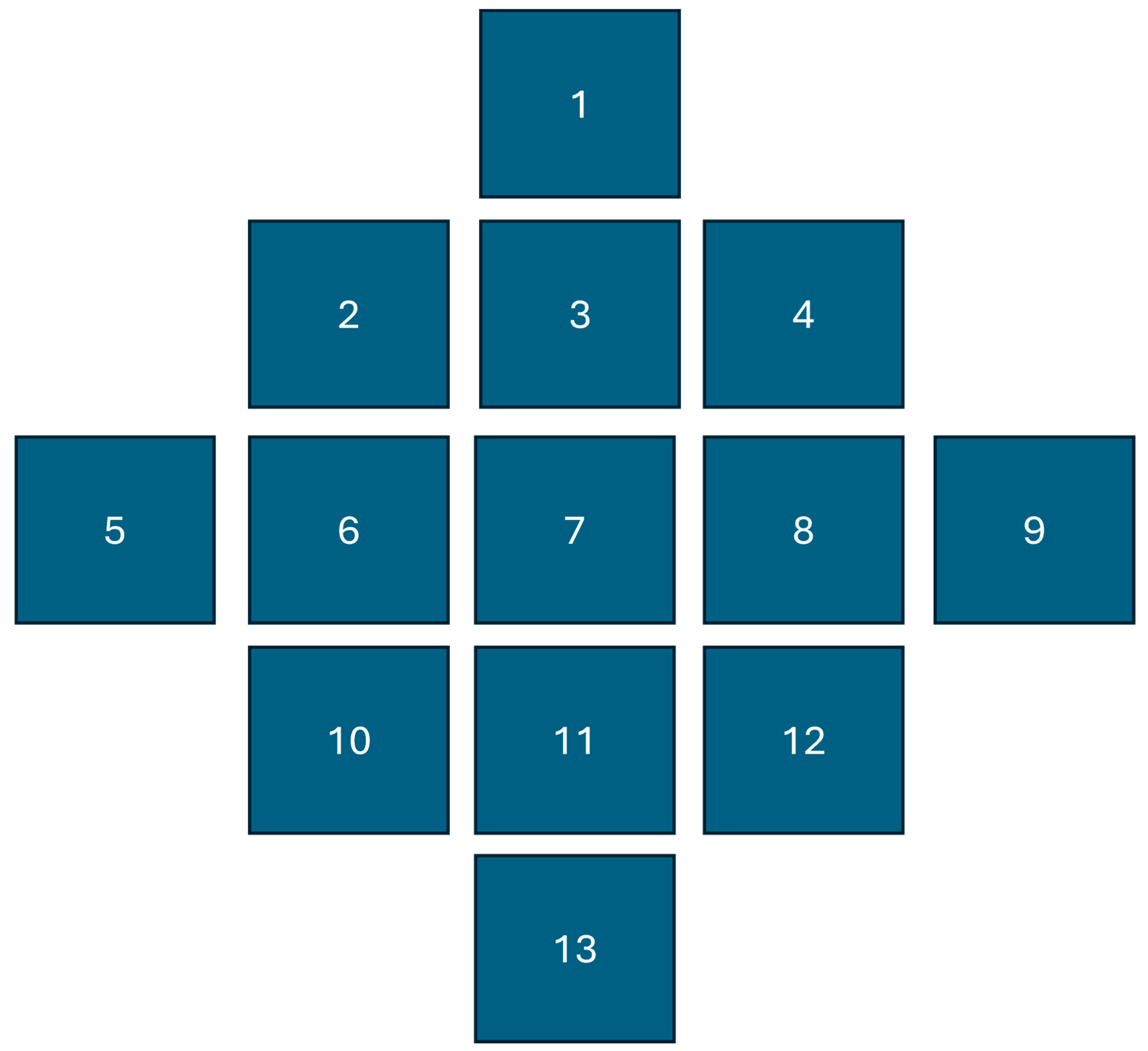
Figure 2.
Spray drone outfitted with spot spray nozzle hovering over the center of the targeted area.
Figure 2.
Spray drone outfitted with spot spray nozzle hovering over the center of the targeted area.
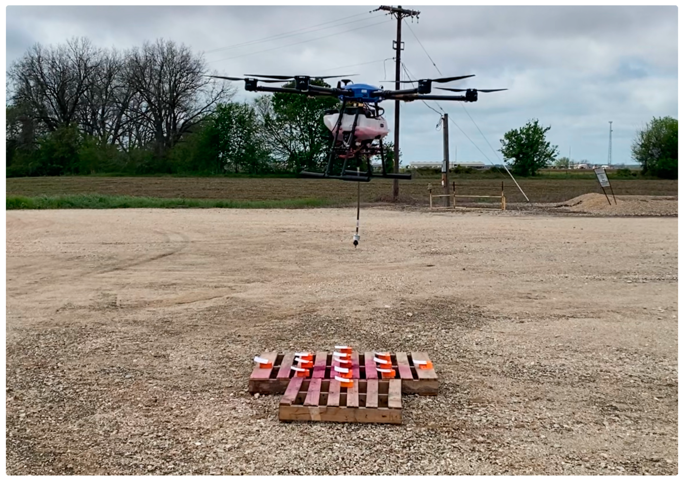
Figure 3.
Spray drone configuration showing rotors, arms and single spot spray nozzle placement.
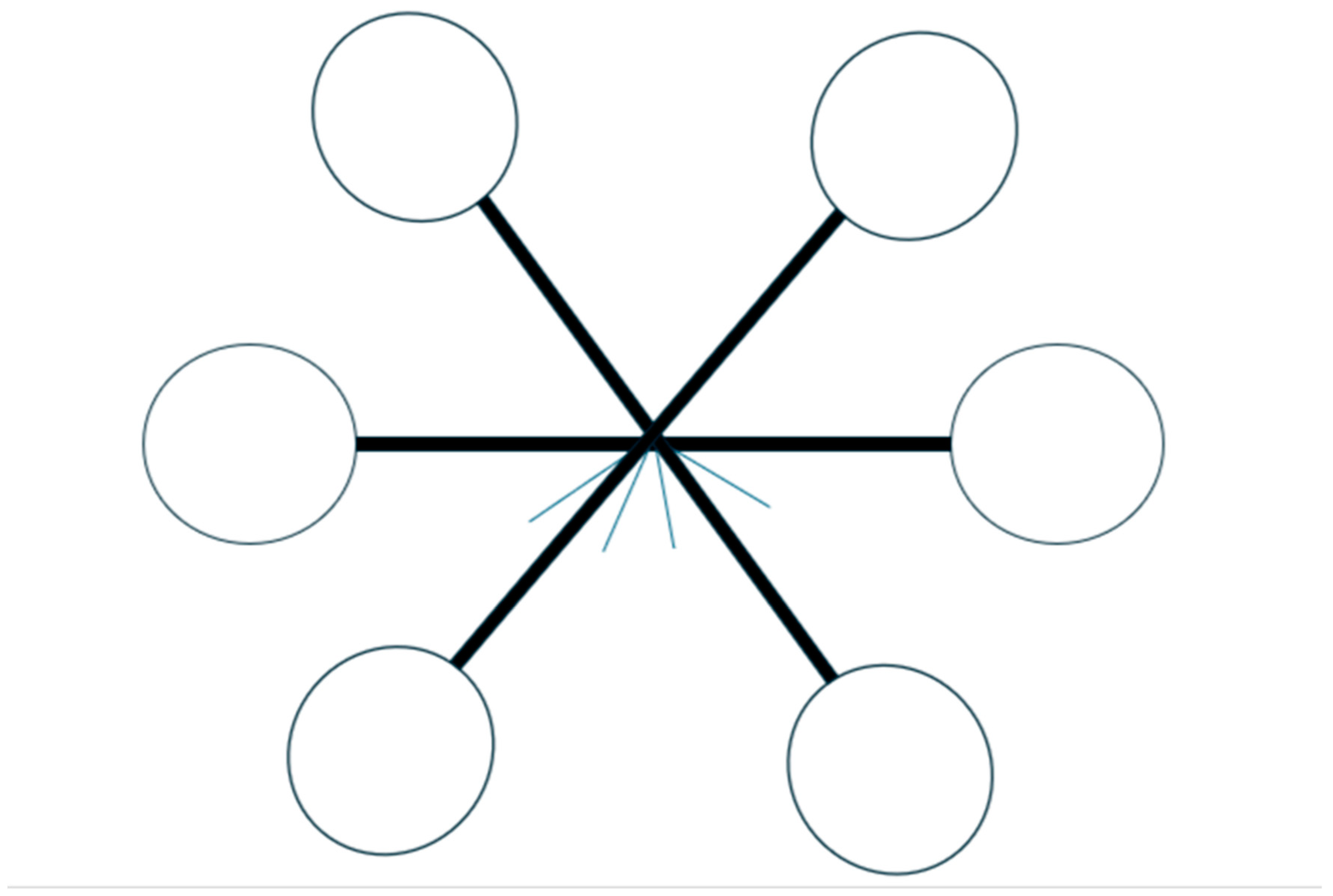
Figure 4.
Spot spraying nozzle (30°) with drop tube and washers.
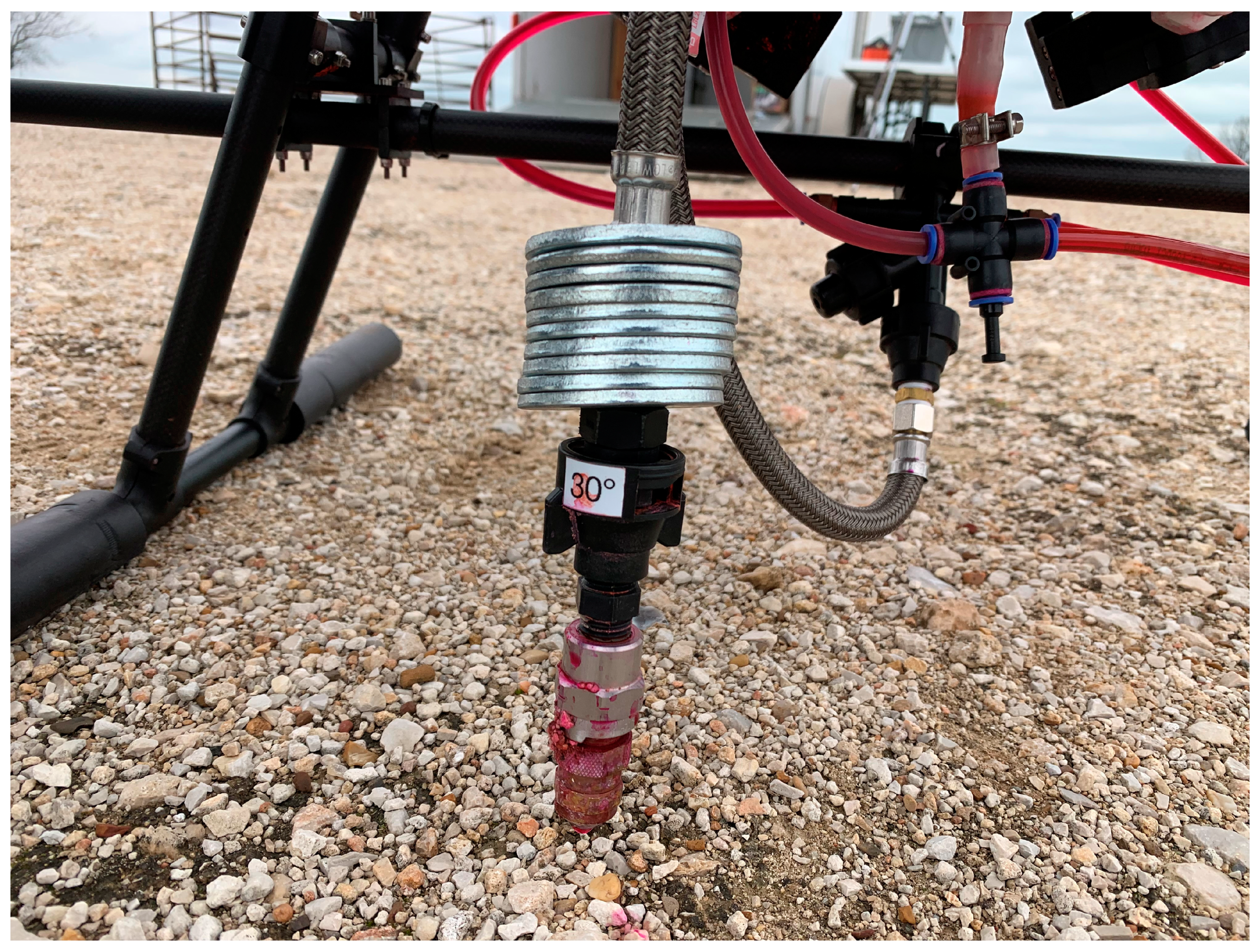
Figure 5.
Topographic heat map showing spray deposition and center of deposition (centroid).
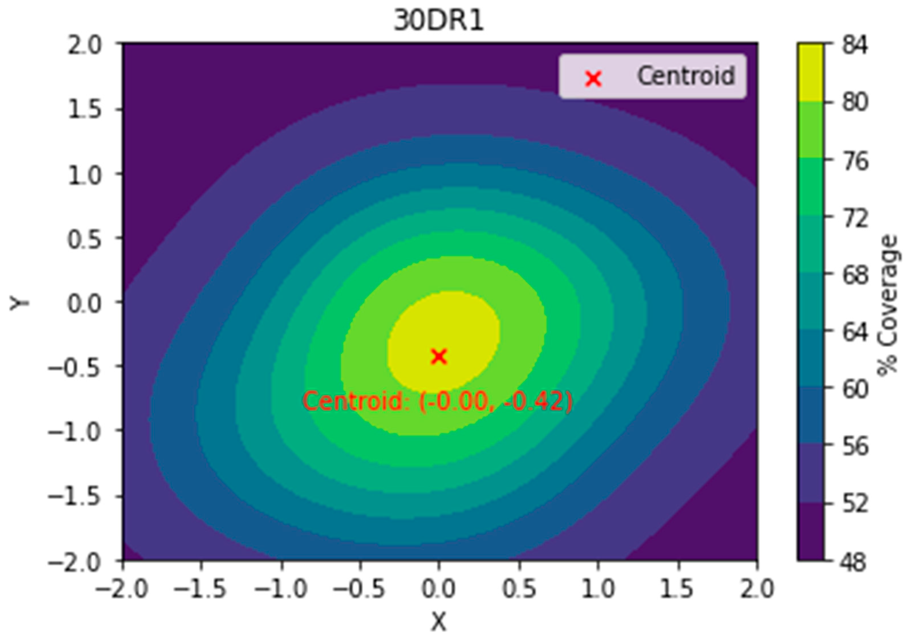
Figure 7.
Analysis of spray displacement for 0°angle. The comparison circles on the right show that when the circles intersect and the angle of intersection (<90°), the means are significantly different (Tukey’s HSD Test at P=0.05).
Figure 7.
Analysis of spray displacement for 0°angle. The comparison circles on the right show that when the circles intersect and the angle of intersection (<90°), the means are significantly different (Tukey’s HSD Test at P=0.05).
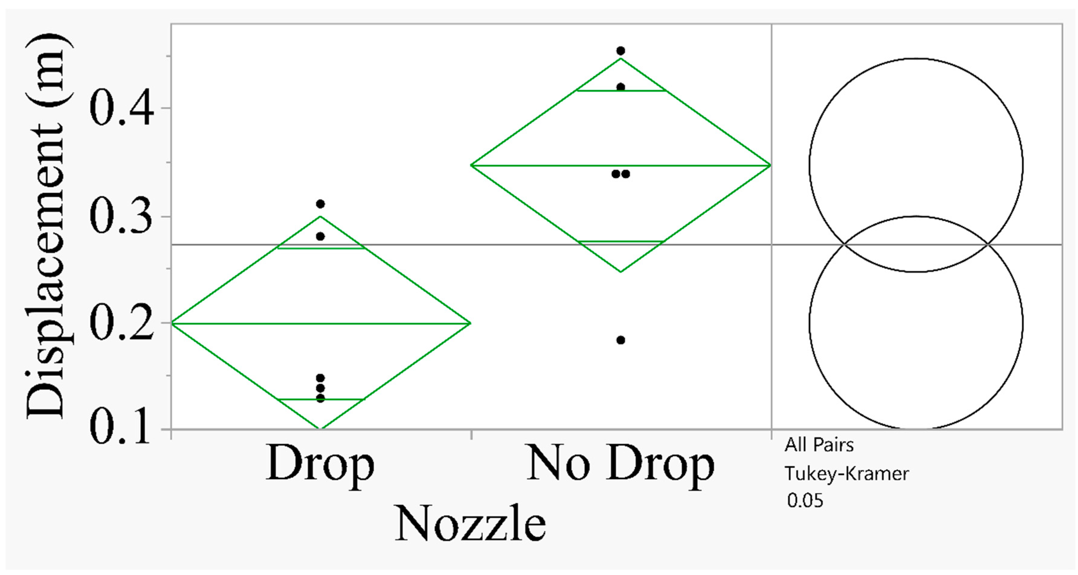
Figure 8.
Analysis of spray displacement for 30°angle. The comparison circles on the right shows that when the circles intersect and the angle of intersection (<90°), the means are significantly different (Tukey’s HSD Test at P=0.05).
Figure 8.
Analysis of spray displacement for 30°angle. The comparison circles on the right shows that when the circles intersect and the angle of intersection (<90°), the means are significantly different (Tukey’s HSD Test at P=0.05).

Figure 9.
Relationship between spray displacement and wind speed for Drop vs No Drop nozzle.
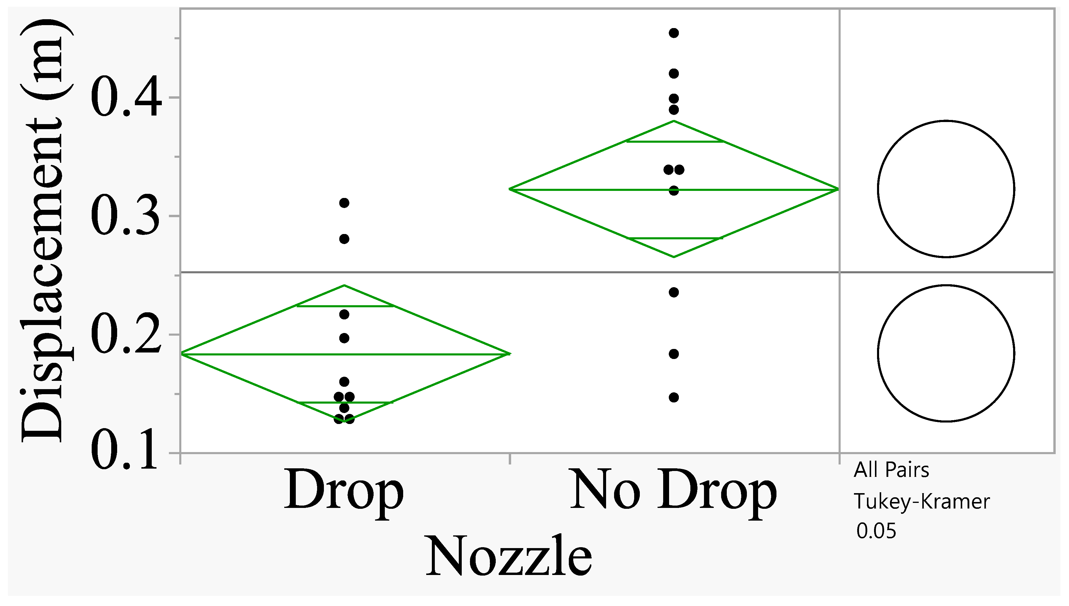
Figure 11.
Comparison of slopes using ANOM Method (Quantile=2.11991; adjusted degrees of freedom =16; Adjustment=Nelson).
Figure 11.
Comparison of slopes using ANOM Method (Quantile=2.11991; adjusted degrees of freedom =16; Adjustment=Nelson).
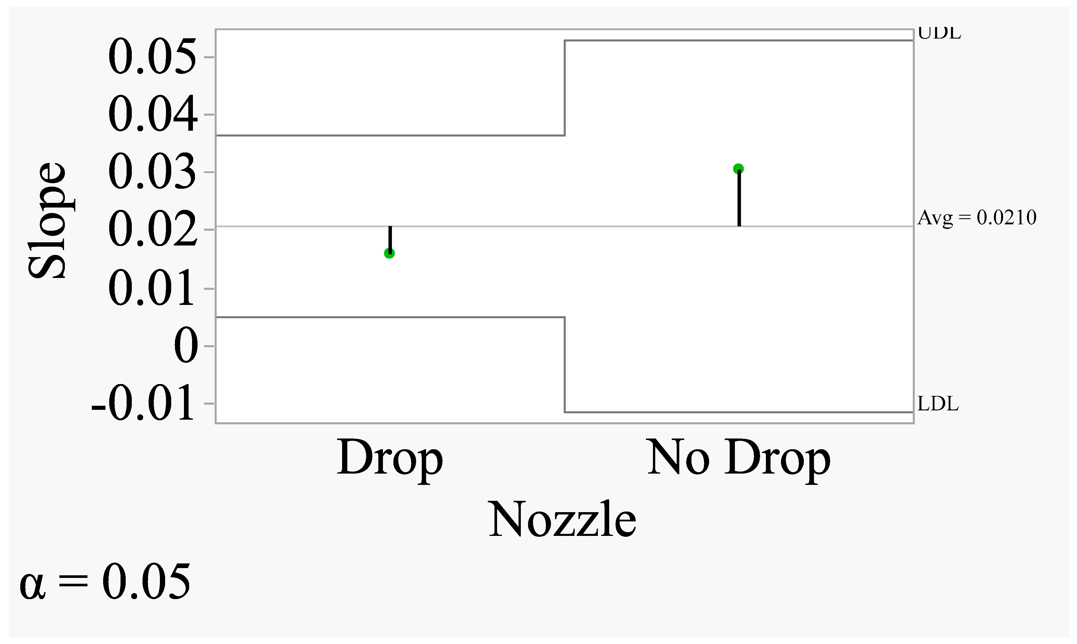
Figure 12.
Regression of displacement (m) on wind speed for the 0° and 30° angle nozzles.
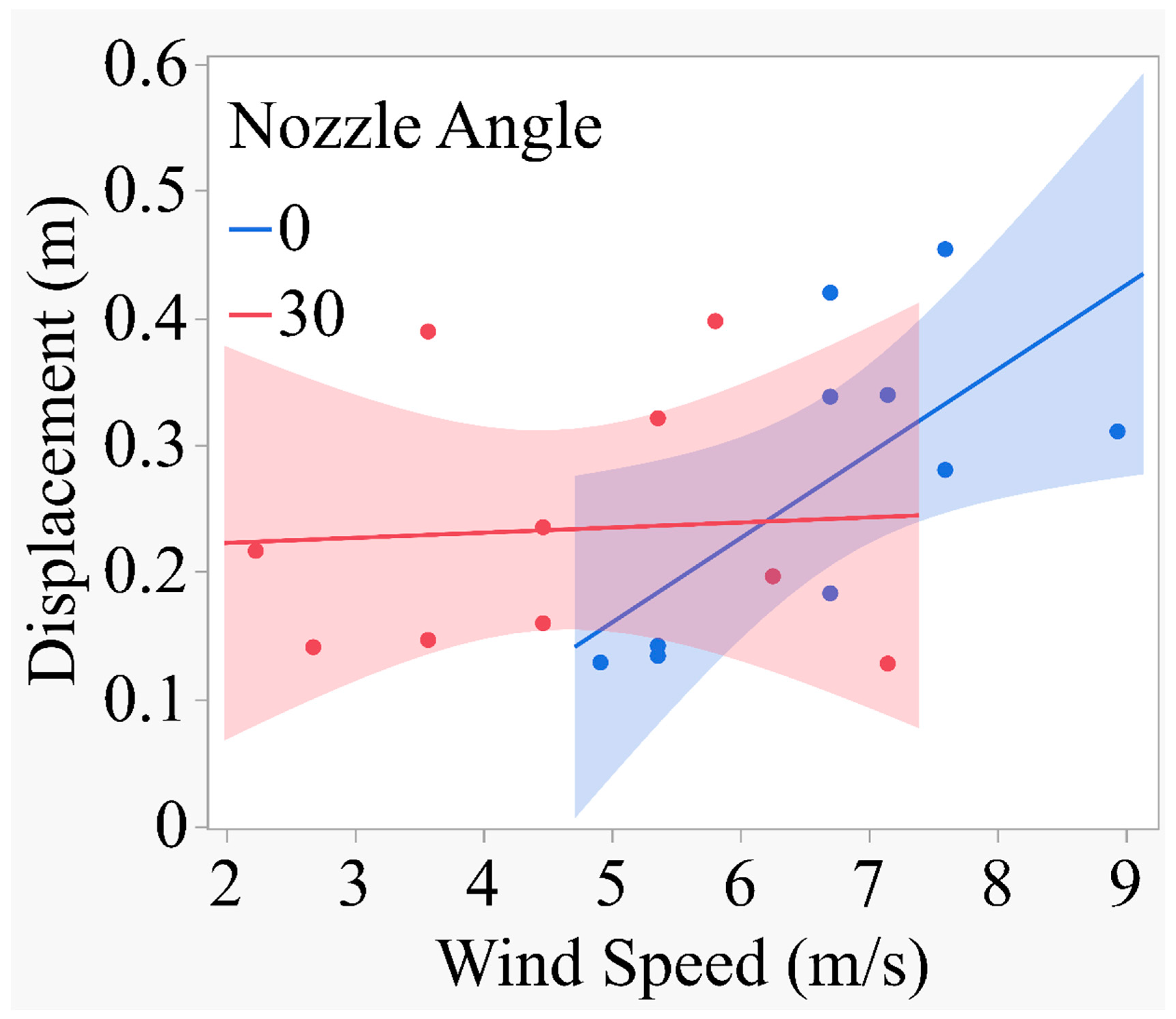

Table 1.
Descriptions of treatments used in the study.
| TRT | Angle | Drop | Rep |
| 1 | 0 | No Drop | 1 |
| 1 | 0 | No Drop | 2 |
| 1 | 0 | No Drop | 3 |
| 1 | 0 | No Drop | 4 |
| 1 | 0 | No Drop | 5 |
| 2 | 0 | Drop | 1 |
| 2 | 0 | Drop | 2 |
| 2 | 0 | Drop | 3 |
| 2 | 0 | Drop | 4 |
| 2 | 0 | Drop | 5 |
| 3 | 30 | No Drop | 1 |
| 3 | 30 | No Drop | 2 |
| 3 | 30 | No Drop | 3 |
| 3 | 30 | No Drop | 4 |
| 3 | 30 | No Drop | 5 |
| 4 | 30 | Drop | 1 |
| 4 | 30 | Drop | 2 |
| 4 | 30 | Drop | 3 |
| 4 | 30 | Drop | 4 |
| 4 | 30 | Drop | 5 |
Table 2.
Metereological conditions during the test peroiod using straight stream nozzles (0°).
| Meteorological parameter | No Drop Nozzle | Drop Nozzle | ||||||||
| R1 | R2 | R3 | R4 | R5 | R1 | R2 | R3 | R4 | R5 | |
| Wind Speed (m/s) |
6.7 |
6.7 |
6.7 |
7.6 |
7.2 |
5.4 |
4.9 |
5.4 |
8.9 |
7.6 |
| Wind Direction | N | N | N | N | N | N | N | N | N | N |
| Temp(C) | 17.2 | 17.2 | 17.2 | 17.8 | 17.2 | 16.1 | 16.1 | 16.1 | 16.1 | 16.1 |
Table 3.
Metereological conditions during the test peroiod using straight stream nozzles (30°).
| Meteorological parameter | No Drop Nozzle | Drop Nozzle | ||||||||
| R1 | R2 | R3 | R4 | R5 | R1 | R2 | R3 | R4 | R5 | |
| Wind Speed (m/s) |
3.6 |
3.6 |
5.8 |
4.5 |
5.4 |
7.2 |
2.2 |
4.5 |
2.7 |
6.3 |
| Wind Direction | S | S | S | S | N | N | S | S | S | N |
| Temp(C) | 27.8 | 29.4 | 30.0 | 30.0 | 17.8 | 17.2 | 27.8 | 27.8 | 27.8 | 17.2 |
Table 3.
Analysis of spray droplet parameters to test homogeneity of variance using Levene’s Test.
| Droplet Parameter | 0° | 30° | ||||
| F | P | Df* | F | P | Df | |
| % Coverage | 5.24 | 0.02 | 1, 117 | 0.27 | 0.60 | 1, 117 |
| Droplet Density | 5.24 | 0.02 | 1, 108 | 0.27 | 0.60 | 1, 117 |
| Dv0.1 | 6.57 | 0.01 | 1, 107 | 7.46 | 0.0073 | 1, 111 |
| Dv0.5 | 1.65 | 0.20 | 1, 107 | 3.87 | 0.05 | 1, 111 |
| Dv0.9 | 5.09 | 0.03 | 1, 107 | 0.34 | 0.56 | 1, 111 |
| Relative Span | 2.56 | 0.11 | 1, 107 | 0.39 | 0.53 | 1, 111 |
*Degrees of freedom.
Table 4.
Spray droplet characteristics for the spray deposits on artificial collectors using straight stream and 30°full cone drop nozzles.
Table 4.
Spray droplet characteristics for the spray deposits on artificial collectors using straight stream and 30°full cone drop nozzles.
| 0° | 30° | |||||||
|
Nozzle |
% Area Coverage (x̄±SEM)* | % Area Coverage (x̄±SEM) | ||||||
|
Mean |
F |
P |
Df |
Mean |
F |
P |
Df |
|
| Drop | 11.60±2.50a | 0.47 | 0.49 | 1, 80.7 | 28.13±4.38a | 0.17 | 0.68 | 1, 115.2 |
| No Drop | 14.82±3.94a | 30.76±4.67a | ||||||
| Droplet Density (Drops/cm2) | Droplet Density (Drops/cm2) | |||||||
| Drop | 74.87±16.13a | 0.52 | 0.47 | 1, 108 | 181.50±28.18a | 0.17 | 0.68 | 1, 117 |
| No Drop | 95.59±25.44a | 198.47±30.11a | ||||||
| Dv0.1, µm | Dv0.1, µm | |||||||
| Drop | 248.47±6.43a | 0.04 | 0.85 | 1, 107 | 254.57±16.52b | 9.64 | 0.002 | 1, 111 |
| No Drop | 246.11±11.56a | 342.66±24.11a | ||||||
| Dv0.5, µm | Dv0.5, µm | |||||||
| Drop | 448.40±12.44a | 0.31 | 0.58 | 1, 107 | 448.24±25.93b | 8.86 | 0.0036 | 1, 111 |
| No Drop | 437.36±15.76a | 574.10±34.42a | ||||||
| Dv0.9, µm | Dv0.9, µm | |||||||
| Drop | 628.53±15.39a | 2.83 | 0.09 | 1, 107 | 616.59±28.13a | 3.88 | 0.05 | 1, 111 |
| No Drop | 582.87±23.65a | 703.64±34.74a | ||||||
| Relative Span | Relative Span | |||||||
| Drop | 0.85±0.02a | 5.19 | 0.02 | 1, 107 | 0.87±0.03a | 17.13 | 0.0001 | 1, 111 |
| No Drop | 0.76±0.03b | 0.68±0.03b | ||||||
* Means within each column followed by the same lower-case letter are not significantly different (Tukey’s HSD Test) at P=0.05.
Disclaimer/Publisher’s Note: The statements, opinions and data contained in all publications are solely those of the individual author(s) and contributor(s) and not of MDPI and/or the editor(s). MDPI and/or the editor(s) disclaim responsibility for any injury to people or property resulting from any ideas, methods, instructions or products referred to in the content. |
© 2024 by the authors. Licensee MDPI, Basel, Switzerland. This article is an open access article distributed under the terms and conditions of the Creative Commons Attribution (CC BY) license (http://creativecommons.org/licenses/by/4.0/).
Copyright: This open access article is published under a Creative Commons CC BY 4.0 license, which permit the free download, distribution, and reuse, provided that the author and preprint are cited in any reuse.


