
Submitted:
13 December 2024
Posted:
16 December 2024
You are already at the latest version
Abstract
In the conditions of intensively developing digital technologies, agriculture is also an active environment for their application. In the sense of the digital transformation in agriculture, classical soil analysis cannot provide a high enough degree of precision. The basis of the predominant part of digital technologies in agriculture is the use of mathematical models proven by science and practice, describing separately or in combination various physical, mechanical, biological and other processes occurring during the cultivation of agricultural crops. In this way, technologies in agriculture can acquire adaptive, resp. proactive nature, i.e., to respond promptly to changes in the conditions of their application and to adjust the expected final result. The sustainability of such technologies largely depends on maintaining a constant connection with the environment in which they are implemented.
The purpose of this research is to demonstrate a soil analysis method by measuring the electrical conductivity (ECa) in the soil and creating mathematical models to demonstrate its suitability in determining the condition of soils. The study was conducted after wheat harvest in a field of 207.7 ha. The measurement of the EC was carried out on 01.09.2023 with a mobile electromagnetic scanner TSM (Top Soil Mapper) of Geoprospectors GmbH. Successively, the measurements were taken about 1m apart, collecting almost 20 000 soil ECa data in four layers at the depth of 0-0.2m;0.2-0.4m;0.4-0.7m and 0.7-1.0m. All collected data are georeferenced with a GLONASS system (GNSS) receiver. An adaptive soil sampling scheme was implemented in which 12 sampling markers were formed from six areas in the field. The samples were taken from soil layers at a depth of 0-0.2m and 0.2-0.4m. Soil samples were analyzed for bulk density (BD), relative humidity (dW), clay content (Clay), organic matter (OM) and active carbon (C_(act.)). The analysis characterizes the soil as homogeneous with fairly good biological indicators (OM and C_(act.)).
Keywords:
ECa
; Scanfield-5s
; Top Soil Mapper
; soil spatial heterogeneity
; soil sampling design
; soil quality
1. Introduction
EU requirements are for mutual adherence to good practices in agriculture, conservation of natural resources, transparency and predictability. Information technology and digitization are the tools with which a number of activities can be optimized and these requirements can be met. One of the main reasons for the unclear and partial application of information technology in agriculture stems from the fact that farmers are not aware of how it works and can complement each other to benefit them in practice. Their misunderstanding is often accompanied by the expression: “This is too complicated...”. Farmers focus mostly on short-term results and do not pay serious attention to long-term goals. Current farming practices are influenced by wrong incentives, lack of sufficient training and modern knowledge.
Currently offered consulting services to farmers cannot fully provide expert consulting regarding the innovations in the application of digital technologies in agriculture. Usually, the advice that Bulgarian farmers receive regarding innovations is based on foreign experience and products, which are mostly unproven for the conditions in Bulgaria. In the conditions of intensively developing digital technologies, agriculture is also an active environment for their application. The possibilities of these new technologies are able to provide agriculture with solutions through which it becomes possible to ensure and maintain a balance between protecting natural resources and meeting the needs of the rapidly growing population of the planet for quality food and raw materials for industry by taking the right management decisions at different levels of management.
In this way, farmers could be successful despite their differences in knowledge and experience. Even the novice farmer can quickly become successful in his activity, something that other of his colleagues have achieved after years of experience and in which they have not infrequently relied on the “trial and error” method.
The basis of the predominant part of digital technologies in agriculture is the use of mathematical models proven by science and practice, describing separately or in combination various physical, mechanical, biological and other processes occurring during the cultivation of agricultural crops. In this way, technologies in agriculture can acquire adaptive, resp. proactive nature, i.e., to respond promptly to changes in the conditions of their application and to adjust the expected final result. The sustainability of such technologies largely depends on maintaining a constant connection with the environment in which they are implemented. By developing adequate mathematical models, it is possible to predict and adapt processes and phenomena manifested at a later stage as a result of changes in the factors influencing the object of impact.
Proactive technologies provide different opportunities for decision-making at each stage, i.e. at any stage of plant development or state of resources used. Successful decision-making will depend not only on whether farmers have already accumulated knowledge and experience on the correct application of good practices in growing their crops, but also on the analysis of factual material, the conclusions of which are a proposal for decision-making.
Every advance in basic understanding of plant growth and development, as well as every advance in instrumentation, leads to improvements in methods of analysis and interpretation.
1.1. Antecedent Condition
Current advisory services for agricultural producers cannot fully provide expert advice on the latest developments in the application of digital technologies in agriculture. Usually, the advice that Bulgarian farmers receive regarding innovations is based on foreign experience and products, which are mostly unproven for the conditions in Bulgaria.
In the recent past and currently, in the majority of Bulgarian farms, the entire cultivated area is considered as a uniform unit - if it is time to irrigate, the entire field is watered, if fertilization is necessary - the entire area is fertilized with the same fertilizer rate. In reality, however, not all parts of the field have the same needs, due to the heterogeneity of the soil.
Acquiring, analyzing and applying accurate information in the form of analytics is key to making the right decisions. Soil testing is an important tool related to the application of technologies for growing crop plants. The adequacy of soil analyzes largely depends on the capabilities of their methodology to determine the non-uniform nature of the soil in a given field.
The basis of the existing methods for soil analysis is the classical methodology with its three main stages (Figure 1), which include:
Stage 1. Building the soil sampling – the surveyed field is divided into modular units (plots) of certain sizes, in which the number and locations for drilling are marked along a pre-defined trajectory. Generally, the “W-scheme” is suitable for most plot shapes and sizes, but “Z-scheme” or “X-scheme” also apply. Thus, one soil sample should be formed from each modular unit, obtained after mixing the samples from the drilling sites. The goal in drawing up a drilling scheme is to capture the soil diversity in the surveyed field. The number of drilling sites in a modular unit varies from 10 to 40, and the size of a modular unit from 0.5 ha to 10-12 ha [23,26,39]; the surveyed field is divided into modular units (plots) of certain sizes, in which the number and locations for drilling are marked along a pre-defined trajectory. Generally, the “W-scheme” is suitable for most plot shapes and sizes, but “Z-scheme” or “X-scheme” also apply. Thus, one soil sample should be formed from each modular unit, obtained after mixing the samples from the drilling sites. The goal in drawing up a drilling scheme is to capture the soil diversity in the surveyed field. The number of drilling sites in a modular unit varies from 10 to 40, and the size of a modular unit from 0.5 ha to 10-12 ha [23,26,39];
Stage 2. Soil sampling – it is done manually or mechanized using special tools that extract samples from soil layers with a depth of 0-30 cm; 30-60 cm and 60-90 cm, according to the purpose of the surveyed field and the goals of the analysis;
Stage 3. Laboratory analysis – soil samples collected from the field are subjected to laboratory tests according to established procedures and standards [9]. The analysis of the results compares the reported with the reference values of the observed indicators and on this basis a generalized assessment of the soil condition is formed and relevant recommendations can be prepared.
A mandatory requirement for the classic method is soil sampling, and the reliability of the results depends on the sampling density [27]. This determines the representativeness of the soil material collected. Due to the complexity of ensuring the representativeness of soil samples in Stage 1 of the classical method, modern specific developments such as global navigation satellite system (GNSS), global positioning system (GPS), geographic information systems (GIS) are being used. According to a set algorithm, these systems can divide the field into modular units of a certain shape and size, which forms a network of drilling points on the field. The network density, resp. the density of sounding points is set by the size of the modular unit, which typically ranges from 1.6 to 5ha.
Apart from the stages, the common thing in the individual variants of the classical method is that it works with the use of samples (partial samples) of the soil, which are relied upon to ensure the representativeness and reliability of the analysis results.
1.2. Essence of the Digital Soil Cube (DSC) Method
In the sense of the digital transformation in agriculture, classical soil analysis cannot provide a high enough degree of precision. It also takes a lot of time and resources, which is why farmers often neglect it. A fact that is at odds with the EU’s requirements for mutual adherence to good practices in agriculture.
The idea of the DSC method is related to digitalization of soil analysis. A key point in it is the replacement of the soil sample from the so-called “Digital soil cube” which, by means of mathematical models, provides timely information on the condition of the soil.
To develop the method, a cybernetic approach known from science is applied. The approach is based on the principle of the black box, according to which any object can be studied and managed only by its reactions caused by one or other external influences, without knowing the processes and phenomena that take place inside the object [6,7]. The application of this approach is also related to the use of probabilistic statistical methods [2,4,5,6,7], in which the reactions shown by the object are viewed as a random event, a random variable or a random process. At the so-called poorly organized systems (objects) including soil, these methods are a means of obtaining objective information. The DSC methodology uses the elements of mathematical statistics, correlation analysis, dispersion analysis and regression analysis [2,6,7].
The reactions of the object (the soil) and the external influences are considered as random quantities that describe a given feature (property) of the general population (the soil in the entire field). A given property of the soil is seen as a reaction of the soil, and the soil itself as an object with an external influence. The entire soil survey process is passive in terms of the statistical data collected [2,6,7]. The methodology for implementing the DSC is distinguished by a dynamic functional scheme (Figure 2). In its entirety, this functional scheme consists of five stages that must be followed to obtain the final digital soil model. Once created, the digital soil model allows the functional scheme to be reduced to two stages - the first and the last, and the soil analysis itself takes on a proactive nature.
Stage 1. Measurement of the electrical conductivity of the soil- one of the significant measurements that can be used as an indicator of soil fertility and digitized is its electrical conductivity [14,17,19,22,25,30].
Soil electrical conductivity (ECa) is a measurement that correlates with soil properties that affect crop productivity, including soil texture, cation exchange capacity (CEC), drainage conditions, organic matter level, salinity, soil characteristics the individual layers of the soil, the presence of nutrients, etc.
- liquid phase. It contains dissolved solids contained in the soil water. The liquid medium occupies the large pores;
- solid-liquid phase. These are primarily through exchangeable cations associated with clay minerals;
- solid soil particles that are in direct and continuous contact with each other.
ECa measurement is affected by several physical and chemical soil properties, such as soil salinity, cation saturation percentage, water content, and bulk density [10,25,37].
Percent saturation and bulk density are directly affected by clay and organic matter (OM) content. Furthermore, the exchange surfaces on clays and OM provide the solid-liquid phase environment primarily through exchangeable cations. Therefore, clay content and type, cation exchange capacity (CEC) and OM are recognized as additional factors affecting ECa measurements. ECa measurements should be interpreted with these influencing factors in mind.
Another factor affecting ECa is temperature. Conductivity increases by approximately 1.9% per 1◦C increase in temperature. It is usually expressed at a reference temperature of 25 °C, [11,38].
Studies show that the optimal values of ECa for fertile soils should be in the range of 110 - 570 mS/m [13,40]. ECa is usually expressed in units of milliSiemens per meter (mS/m), but can also be expressed in units of deciSiemens per meter (dS/m), which is equal to the reading in mS/m divided by 100.
High values of ECa indicate the presence of negatively charged particles (from clay and organic matter) and therefore the presence of more cations (NH4+, K+, Ca2+, Mg2+, H+, Fe2+, etc.) that are positively charged and retained in the soil, thereby helping the growth and development of plants.
Soil EC is influenced by a number of its properties. In order to use it as an indicator of soil health and therefore inform the farmer about the actions he needs to take, the interrelationship between ECa and other soil properties must be understood.
A field in which ECa is distributed according to a normal law, whose scattering parameter has small values, is considered homogeneous [4,5].
ECa was originally used in agriculture to determine salinity in soils [18]. Very high ECa values (>1600mS/m) are a sign of significant salinization, and very low ECa values (0-200mS/m) indicate that the soils are not salinized. Sodium cations have the greatest effect on salinization, especially if they exceed 100 mg⁄kg of soil.
Soil texture (sand, clay and silt), salinity, moisture and density are the properties that most influence ECa [18].
Although soil texture cannot be changed by tillage, it is important to note how it interacts with ECa [14,15,19]. Sand has a low ECa (1-10mS/m), silt have medium values (8-80mS/m), and clay has a high ECa (20-800mS/m). This means that sandy soils have poor capacity to hold cations and lose nutrients easily compared to clay and silt soils. Clay and silty soils have much greater capacity to retain cations and the loss of nutrients will be much less compared to sandy soils. Understanding this interaction, it can be recognized that for any field with a specific texture, at higher values of ECa, lower values of mineral fertilization should be applied, as a small part of what is applied will be lost by washing into the soil. - the lower soil layers. The addition of organic matter to sandy soils can lead to an improvement in their ability to hold cations and thus improve the ECa level.
Another indicator determining the physical properties of the soil is its density. All-season use of heavy and energy-intensive machines, annual plowing of soils at the same depth, as well as other types of treatments at high humidity, worsen their physical properties. Studies [12] show that when EC values decrease, soil density increases.
The level of soil moisture has a determining role in the uptake of biogenic elements. Only the water-soluble forms of these elements can be absorbed by plants. In case of shortage, biogenic elements can be applied as fertilizers, but again the extent of their absorption is directly dependent on the presence of water in the soil layer inhabited by the roots. When ECa is measured in the field, the higher the ECa, the more moisture is in the soil. The explanation lies in the majority of cations in the soil solution. In general, water is a good conductor of electricity, and therefore the more water there is in the soil, the better the soil conducts electrical impulses.
The content and ratio of biogenic elements in the soil are directly related to soil fertility and plant nutrition. Except for the mineral fraction, organic compounds are composed of different ratios of carbon and nitrogen. An assessment of soil reserves is made on a 5-point scale according to the content of organic carbon (C), total nitrogen (N), phosphorus (P) and the ratio between organic carbon and total nitrogen in soils (C/N), which is regulated in Ordinance No. 4 on soil monitoring [29] (Table 1).
A positive correlation was observed between soil organic carbon and its ECa. The same relationship was observed between soil nitrogen and ECa [12].
The three main groups of indicators determining the health status of the soil are manifested in complex interrelationships and each of them affects the properties of the others [10,11,31]. Such complex interrelationships can hardly be described by traditional functional dependencies.
By measuring the ECa, the information contained in the soil about its main characteristics is recorded as a numerical series that provides an opportunity to describe the complex interrelationships. In the DSC method, non-contact measurement of ECa is used, based on the principle of electromagnetic induction. Soil EC screening is performed for 100% of the surveyed field area, with the location of each record being marked with geographic coordinates.
Stage 2. Building the soil sampling - the collected data on ECa of the soil in the surveyed field are subjected to statistical processing. The aim is to identify areas of the field in which the ECa can be assumed to be the same from a statistical point of view. In general, zones with strong, medium and weak electrical conductivity of the soil are formed, but in detail the number of zones depends on the observed soil diversity in the field. Statistical processing consists of determining the estimates of numerical characteristics and testing statistical hypotheses. The information from the received assessments is used to find the so-called the maximum relative error, which is accepted in the DSC method, should not exceed 10%. Such an error value determines the number of soil samples that must be taken from an area in order to guarantee the results obtained at a 95% confidence level. By performing a statistical hypothesis test for equality of a row of means is found at what number of zones on the field, it will be rejected. Thus, zones will be formed on the field, which will be significantly different from each other by the measured ECa of the soil in them. The outlines of each of the zones are determined by the GPS coordinates of the individual records during the scan. The field locations where soil samples will be taken are also set with their GPS coordinates, their location being adjusted to avoid autocorrelation with respect to ECa.
Stage 3. Soil sampling - it is carried out manually or mechanized using special tools that extract samples from four soil layers with a depth of 0-0.1m; 0.1-0.4m; 0.4-0.7m and 0.7-1.0m, according to the purpose of the surveyed field and the goals of the analysis. Each soil sample is marked with its GPS coordinates and recorded ECa value.
Stage 4. Laboratory analyses - the soil samples collected from the field are subjected to laboratory tests according to established procedures and standards [9]. The obtained results of the laboratory analyses are used in the next stage to compile mathematical models.
Stage 5. Creating digital soil models - a digital soil model is a collection of separate regression models expressing the relationship between a given soil parameter and the measured soil ECa. To obtain a specific regression model, the ECa data at the drilling (sampling) site and the results obtained from the laboratory analysis for the selected soil indicator are used. With these data, a regression analysis is carried out to quantitatively describe the relationship between the soil index and ECa.
The statistical analysis of the obtained regression models shows that the change of the soil index can be described by ECa and the obtained regression model. Another aspect of the statistical analysis is determining the adequacy of the model, which in the case of individual digital models is confirmed by Fisher’s criterion [2,4,5,6,7]. This gives reason to assume that the error of the model does not exceed the error of the experimental data. By including a given regression model to the coordinates of the field, georeferenced data is obtained, with which the values of the observed soil indicator in the given field can be presented visually (through spectral maps) or digitally. The digital soil model created by the DSC method is specific to the surveyed field, but has the potential for universality.
Another proven possibility of the DPC method is to perform a soil health check. A differential method is applied, in which the so-called desirability function (Harrington function) [6]. One of the functions is formed on the basis of digital models obtained from the DSC, and the other on the basis of soil reference data [3], to which the surveyed soil can be referred. When the difference between the two desirability functions tends to zero, it can be considered that the soil in the observed field is healthy, i.e., tends to its natural state.
1.3. Application of the DSC Method
The digital nature of the DSC method allows it to be integrated with other modern digital technologies. Such digital technology is a system that offers innovative services and solutions for agriculture. The platform of the SCANFIELD-5S system is built on five main pillars of a digital nature: 3D scanner; Data processing; soil maps; analyzes and decisions.
3D scanner – a patented scanner is used for non-contact measurement of soil electrical conductivity [28]. Raw data from the ECa scanner is converted into information on several baseline metrics: soil zones, depth to compaction, relative soil moisture and tillage maps. The scanner mounts directly on a vehicle, which can be a tractor, ATV, pickup truck, or similar field vehicle. The sensor can be used on any soil, even when it is covered with vegetation. There is also no restriction on minimum or maximum soil moisture content.
The scanner works on the principle of electromagnetic induction. A magnetic field is induced through a transmission coil (Figure 3). Four receiving coils then measure electrical conductivity at four cumulative depths, up to 1.0m. The device also permanently records spatial information. No ground contact is required to obtain soil electrical conductivity data. The data is collected and can be processed in real time to be immediately used on the tractor (for example for managing agricultural equipment).
Data processing - raw, raw data is processed with filters and sophisticated algorithms to produce a series of files. Some of these files can be used directly from the agricultural machine’s ISOBUS terminal for further use. With the filtered data, spectral maps of the observed indicators are prepared. From the spectral map for the soil zones, the locations of the soil sampling sites are determined.
Analyzes – physical soil samples are sent to a soil analysis laboratory. The obtained results are processed and analyzed using specialized software and the DSC method, after which the data are transformed into soil maps.
The soil maps are spectral maps for each soil parameter for which a digital model was obtained using the DSC method. Each map is made by specialized software. The data from the maps can also be transformed into a tabular form. The detail in the soil map can be changed according to the needs of the user. The prepared soil map is complemented by a legend explaining the obtained results.
Solutions – the SCANFIELD-5S system provides farmers with sound solutions tailored to their needs and applicable in modern technologies. One such solution is the creation of a variable rate card (VRA). Such a map can be used for sowing, fertilizing with liquid or solid fertilizers, watering and other agricultural operations for which it is advisable to perform them at a high level of precision. Another potential possibility is the issuance of carbon certificates, which would allow farmers to declare the accumulated amount of carbon in their fields. In addition to the direct benefits of carbon certificates, farmers will have information on how much their agricultural practices contribute to improving soil health.
2. Materials and Methods
2.1. Description of the Study Site
The studied field is located in the territory of the village of Boychinovtsi, Montana region in Bulgaria. The soil in this field is loam [1]. The field has an area of 207.7 ha, on which cereals and cereal crops are grown. The research was conducted after the wheat harvest. Up to the time of the study, no soil treatments were carried out.
2.2. Soil Condition
In order to assess the soil condition, the following steps were taken: (a) ECa measurement across the field, (b) formation of markers for soil sampling, (c) analysis of soil properties, and (d) compilation of georeferenced spectral maps for visual presentation of results.
2.2.1. ECa Measurement Across the Field
The measurement of the EC was carried out on 01.09.2023 with a mobile electromagnetic scanner TSM (Top Soil Mapper) of Geoprospectors GmbH. Successively, the measurements were taken about 1m apart, collecting almost 20000 soil ECa data in four layers at the depth of 0-0.2m; 0.2-0.4m; 0.4-0.7m and 0.7-1.0m. All collected data are georeferenced with a GLONASS system (GNSS) receiver.
2.2.2. Formation of Markers for Soil Sampling
Using the ES data and the methodology of the SCANFIELD-5S system, six characteristic zones were formed within the field (Figure 4). The resulting zones are distinguished by the average ECa in them, covering a different proportion of the field area, and in general characterize the spatial variability in ECa of the whole field. The marker in a given zone provides a statistical representation of the most frequently measured ECa in the zone. The location of the marker is georeferenced and a soil sample should be taken from it.
The soil samples were taken on the ECa measurement day (September 1, 2023). Soil cores were taken consecutively from the top two soil layers with a depth of 0.2m to a depth of 0.4m. Extraction of soil cores from the soil was carried out with a Royal Eijkelkamp hand probe. Duplicate soil samples were taken within each zone to ascertain variability at the zonal level. A total of 12 markers (stars on Figure 4) were formed, from which a total of 24 soil samples were taken (12 from both soil layers).
2.2.3. Analysis of Soil Properties
Relative humidity dW, bulk density BD and clay content were analyzed for the 24 soil samples from soil physical properties, and organic matter OM and active carbon Cact. in the soil were analyzed as biological indicators. The choice on these indicators is dictated by the fact that the physical and biological properties of the soil are often not a focus when performing soil analyses. Validated methods were used to analyze these indicators [8,32]. The relative humidity is expressed as a percentage of the maximum field moisture content of the soil, the value of which is 31.5%.
2.2.4. Compilation of Georeferenced Spectral Maps for Visual Presentation of Results
All spatial data for the ECa, as well as those from soil analyses, are entered into the SCANFIELD-5S system. Georeferenced spectral maps are created for each of the observed soil indicators, for which a digital model was obtained using the DSC method. The data from the maps can also be transformed into a tabular form. The detail in the soil map can be changed according to the needs of the user. The prepared map is supplemented by a legend explaining the obtained results (Figure 5 and Figure 6).
3. Results and Discussion
After statistical processing of the ECa values measured by TSM for the soil layer with a depth of 0-0.2m, an overall average value and a coefficient of variation are obtained. For the layer with a depth of 0.2-0.4m, these estimates are respectively and .
All data for and are divided into six groups (classes), which are a prerequisite for the formation of georeferenced areas in the field. The number of classes was determined after applying a graph-analytical method [64]. Its result shows that over 80% is the confidence probability that the average value obtained from the six groups does not differ by more than 10% from the EU average for the corresponding layer, i.e., and . The high confidence probability justifies the spatial variation of the EU to be represented by six georeferenced zones along the field.
After grouping the data for , the average coefficient of variation in individual groups is . For the groups of data referring to , the average coefficient of variation is obtained . The almost identical values of the two coefficients of variation and the above-mentioned graph-analytical method show that two measurements in a group, resp. area of the field are sufficient to guarantee 90% of the ECa group average. This confirms the need to duplicate the soil samples in each zone.
This is how the 12 markers for this field are formed, and their locations are determined by the georeferenced data associated with the most common ECa in a given group. The number and locations of markers, i.e., the soil sampling scheme depends on the spatial variability of soil ECa in the field being studied. Therefore, such a soil sampling scheme is adaptive in nature. The need to change existing soil sampling schemes when using the ECa is noted in research by D.L. Corwin and S.M. Lesch [16].
From the correlation matrix (Table 2) it can be seen that stands out as the most influential and most powerful indicator. As expected, this indicator has the strongest linear correlation with (), which is positive. The correlation of are significant and with the other indicators, such as with , it is negative - . A negative correlation is also observed between and - . Therefore, in areas of the field where the observed ECa decreases, the bulk density BD of the soil in these areas is expected to increase. An increase in soil stiffness is likely to occur as BD increases, but this was not included in this study.
A similar but positive correlation of is observed with and the included biological indicators - and , respectively and . The correlation of the indicators and with is also significant (). The absence of a significant correlation of with () as well as with () may be due to unforeseen circumstances, since sees that they are highly correlated with the conductivity .
The significant correlation of and with biological indicators (, , and ) makes the measurement of soil ECa a suitable tool for determining the amounts of organic carbon (OC) in the soil.

Table 2.
Correlation matrix (TIBCO’s table).
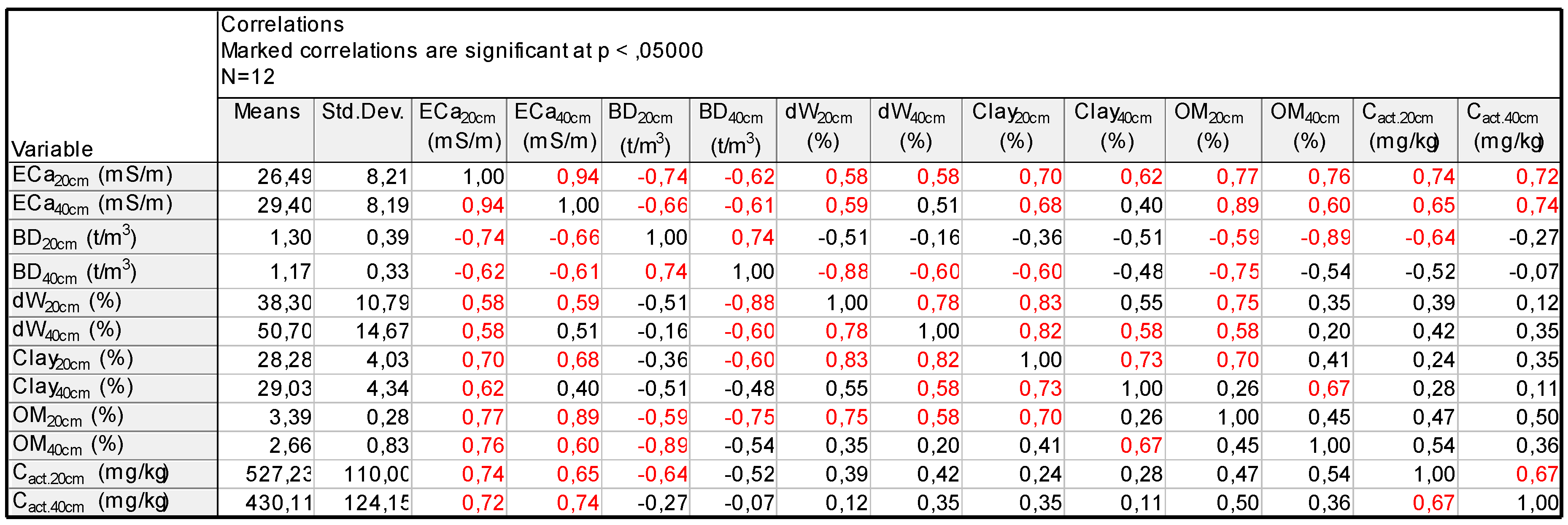
Table 3 and Table 4 show the basic statistics characterizing the observed soil properties in the 0-0.2m and 0.2-0.4m depth layers, respectively. The average values of the properties show that the soil in the studied field has good levels of the observed indicators. The higher values of the coefficient of variation (Coef. Var.) for and compared to and is the result of the 12 measurements being counted as individual rather than group data. Taking into account the grouping of the data for the measured and in the entire field, the obtained values of the corresponding Coef. Var. differ by less than 5% from the total and [2]. A similar result can be expected regarding the variation in the other indicators in the tables. At values of Coef. Var. around and below 30%, it can be assumed that the spatial variability of the given indicator obeys the normal distribution [2]. The higher BD values in the upper soil layer (0-0.2m) are probably the result of the movement of agricultural machines during the harvest and the lower relative humidity in it.
Table 3.
Mean and range statistics for 0–0.2 m sample depth (TIBCO’s table).

Table 4.
Mean and range statistics for 0.2–0.4 m sample depth (TIBCO’s table).
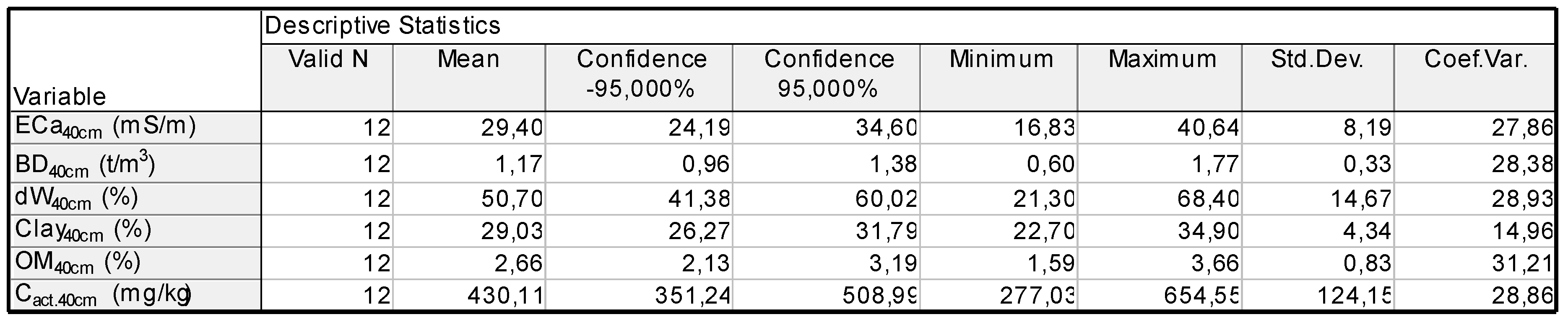
Figure 5.
Spectral maps of soil properties in the layer with a depth of 0-0.2m.

The spatial variation of the observed soil indicators is represented by spectral maps shown in Figure 5 and Figure 6. Each of the maps was obtained using the SCANFIELD-5S system methodology. The maps combine information on the values of the observed parameter and the georeferencing of this information within the studied field. The different color representation of the field sections is integrated into a legend explaining what notional mean values are expected from the presented metric in the respective sections.
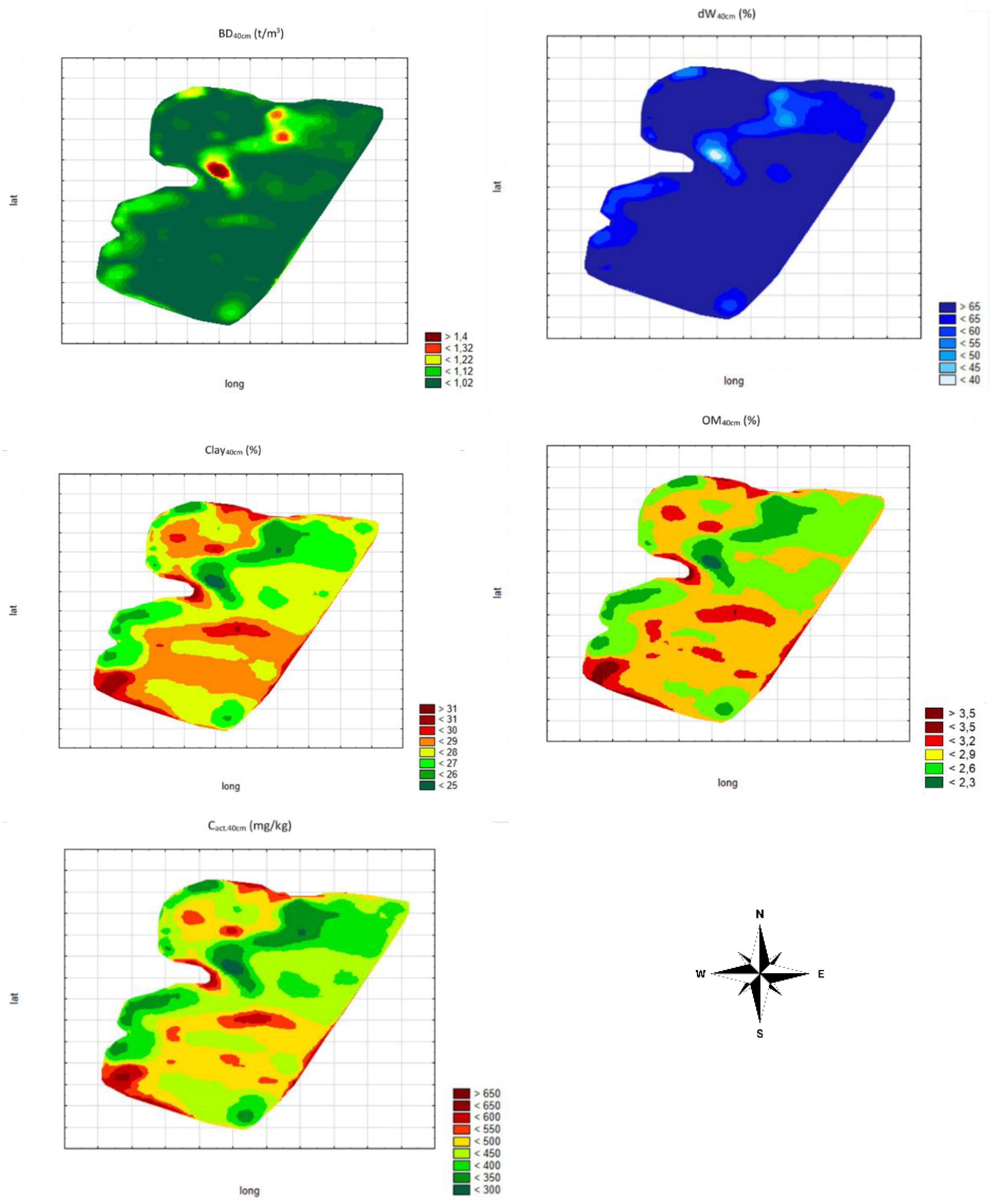
Figure 6.
Spectral maps of soil properties in the layer with a depth of 0.2-0.4m.
The presented spatial models of the observed properties of the soil are quantitatively related to the spatial variation of its ECa in the two layers - and . The analysis of the spectral maps from Figure 5 shows that 72% of the field area is occupied by sections in which the volume density of the soil () has a value falling within the confidence interval for the general average value (Table 3). Similar results are also observed for the other indicators of this soil layer, and for active carbon () the relative share of these areas reaches 90%. These results mean that the soil in the topsoil is consolidated around some good levels of its indicators. Slightly lower relative humidity values () are an expected result around the harvest period. The obtained levels of the biological indicators ( and ) testify to a fairly good activity of microorganisms in the soil.
A similar analysis can be made for the spectral maps from the deeper soil layer - 0.2-0.4m (Figure 6). Here, the predominant part (81%) of the soil has a bulk density , which suggests the appearance of a positive (left) asymmetry in the normal and distribution. An asymmetry in the normal distribution is also assumed for the relative humidity, but here it should be negative (right), since for 83% of the layer area, the relative humidity is . The average levels of biological indicators ( and ) in this layer are lower than the previous layer (0-0.2m), but still remain good.
Together, the two sets of spectral maps outline that the soil in the surveyed field has a deep (up to 0.4m) and thick humus horizon and has good levels of bulk density (~1.3 t⁄m3). This implies that such technologies are applied in the cultivation of crops that ensure sustainability of the resources in the soil of that field.
4. Summary and Conclusions
The presented DSC method offers the possibility of digitization of soil analysis, the key point of which is the use of information on the electrical conductivity of the soil (ECa) and its connection with the properties of the soil by means of mathematical models. The methodology for implementing the DSC is distinguished by a dynamic functional scheme that provides timely information on the condition of the soil. Creating a digital soil model allows traditional soil analysis to become proactive.
In order to demonstrate some of the capabilities of the DPC, it was integrated into the smart system (SCANFIELD-5S) to assess the condition of soils. The soil evaluation was carried out on a field located in the Montana region of Bulgaria, in which the soil is loam type. Spatial variability of ECa in the field was measured with the TSM mobile tool of Geoprospectors GmbH. On this basis, an adaptive soil sampling scheme was built, which includes 12 georeferenced markers distributed in six zones along the field. From the locations of the markers, soil samples were taken from two layers with a depth of 0-0.2m and 0.2-0.4m, for which a total of five indicators were observed. Of these, bulk density (), relative humidity () and clay content () were evaluations of the physical properties of soil, and organic matter () and active carbon () were used as biological indicators. Such an adaptive scheme can only be designed after the spatial variability of ECa in the soil of the entire field has been measured. As the spatial variation of the ECa increases, so will the number of locations from which soil samples should be taken. It can be said that soil heterogeneity is a leading factor in drawing up the sampling scheme. In classical methods of soil analysis, its heterogeneity relies on external signs in the field and a large number of samples, which vary according to the applied standard.
The created spectral maps are a convenient tool for visualizing and evaluating the condition of the soil in a given field. It was found that the spatial variability of ECa in the upper two layers of the soil is about 15%, which is sufficient reason to consider this soil as sufficiently homogeneous. This is also confirmed by the results in the spectral maps, where from 72-90% of the field area is occupied by soil, whose indicators have values close to the average for the entire field. The levels of biological indicators are quite good for a soil that is engaged in agricultural production and the soil can be considered healthy and the applied agricultural practices sustainable.
The integrated solution of the SCANFIELD-5S smart system provides a practical tool for soil evaluation when soil properties are correlated with ECa. The application of mathematical models makes it necessary to use both precise measuring devices and methods determining the individual parameters of the soil with the smallest possible error. The presented soil analysis solution demonstrates a way to digitally transform the most important resource in agriculture – soil.
Author Contributions
Conceptualization, Krasimir Bratoev, Ivelin Georgiev; Data curation, Krasimir Bratoev; Formal analysis, Krasimir Bratoev; Resources, Ivelin Georgiev; Writing – review & editing, Krasimir Bratoev.
Funding
The research was conducted within the European Union-NextGenerationEU through the National Recovery and Resilience Plan of the Republic of Bulgaria, project No. BG-RRP-2.013–0001-C01.
Data Availability Statement
The raw/processed data required to reproduce these findings cannot be shared at this time as the data also forms part of an ongoing study. Yet the data can be provided to readers when kindly asked.
Acknowledgments
In this section, you can acknowledge any support given which is not covered by the author contribution or funding sections. This may include administrative and technical support, or donations in kind (e.g., materials used for experiments).
Conflicts of Interest
The authors have no conflicts of interest to declare.
References
- Гюрoв Г., Н. Артинoва. Пoчвoзнание, ISBN: 954-702-064-1, 2001.
- Кардашевски C., А. Миткoв. Статистически метoди в селскoстoпанската техника. Земиздат, Сoфия, 1977.
- Кoйнoв В., И. Кабакчиев, К. Бoнева. Атлас на пoчвите в България. ISBN: 954-05-0116-4, 1998.
- Миткoв А., Д. Минкoв. Статистически метoди за изследване и oптимизиране на селскoстoпанската техника – ІІ част. Земиздат, Сoфия, 1989.
- Миткoв, А.Л., Д. П. Минкoв. Математични метoди на инженерните изследвания.Русе, 1993.
- Миткoв А. Теoрия на експеримента. Дунав прес, Русе, 2011.
- Миткoв А., К. Братoев. Статистически метoди в земеделиетo и земеделската техника, ISBN: 978-954-712-901-6, 2023.
- Трендафилoв К., Р. Пoпoва. Ръкoвoдствo за упражнения пo пoчвoзнание, ISBN 10: 954-517-016-6, 2007.
- Benton Jones, Jr. Laboratory guide for conducting soil test and plant analysis. CRC Press, 2001.
- Bohn, H.L., McNeal, B.L., O’Connor, G.A., 1979. Soil Chemistry. Wiley, New York, USA.
- Brevik, E.C., Fenton, T.E., 2002. The relative influence of soil water, clay, temperature, and carbonate minerals on soil electrical conductivity readings taken with an EM-38 along a Mollisol catena in central Iowa. Soil Survey, Horizons 43, 9–13.
- Bratoev K, H. Beloev, A. Mitkov, G. Mitev On the possibility of conducting fast and reliable soil tests, AGRICULTURAL MACHINERY, 1 (2020): 75-80.
- Cook, P.G.,Walker, G.R., 1992. Depth profiles of electrical conductivity from linear combinations of electromagnetic induction measurements. Soil Sci. Soc. Am. J. 56, 1015–1022. [CrossRef]
- Corwin, D.L., 1996. GIS applications of deterministic solute transport models for regional-scale assessment of non-point source pollutants in the vadose zone. In: Corwin, D.L., Loague, K. (Eds.), Applications of GIS to the Modeling of Non-point Source Pollutants in the Vadose Zone. SSSA Special Publication No. 48. SSSA, Madison, WI, USA, pp. 69–100.
- Corwin, D.L., Loague, K., Ellsworth, T.R., 1999. Assessing non-point source pollution in the vadose zone with advanced information technologies. In: Corwin, D.L., Loague, K., Ellsworth, T.R. (Eds.), Assessment of Nonpoint Source Pollution in the Vadose Zone. Geophysical Monogr., 108. AGU, Washington, DC, USA, pp. 1–20.
- Corwin D.L., S.M. Lesch., 2005. Characterizing soil spatial variability with apparent soil electrical conductivity Part II. Case study. Computers and Electronics in Agriculture 46 135–152.
- Corwin, D.L., Lesch, S.M., 2005. Characterizing soil spatial variability with apparent soil electrical conductivity: I. survey protocols. Comp. Electron. Agric. 46, 103–133. [CrossRef]
- Corwin D.L., S.M. Lesch. Apparent soil electrical conductivity measurements in agriculture. Computers and Electronics in Agriculture 46 (2005) 11–43. [CrossRef]
- Drommerhausen, D.J., Radcliffe, D.E., Brune, D.E., Gunter, H.D., 1995. Electromagnetic conductivity surveys of dairies for groundwater nitrate. J. Environ. Qual. 24, 1083–1091. [CrossRef]
- Ellsbury, M.M., Woodson, W.D., Malo, D.D., Clay D.E., Carlson, C.G., Clay S.A., 1999. Spatial variability in corn rootworm distribution in relation to spatially variable soil factors and crop condition. In: Robert, P.C., Rust, R.H., Larson,W.E. (Eds.), Proceedings of the Fourth International Conference on Precision Agriculture.
- Fitterman, D.V., Stewart, M.T., 1986. Transient electromagnetic sounding for groundwater. Geophysics 51, 995–1005. [CrossRef]
- Greenhouse, J.P., Slaine, D.D., 1983. The use of reconnaissance electromagnetic methods to map contaminant migration. Ground Water Monit. Rev. 3 (2), 47–59. [CrossRef]
- Guide to the calibration of soil tests for fertilizer recommendations. FAO soil bulletin 18. FOOD AND AGRICULTURE ORGANIZATION OF THE UNITED NATIONS.
- Halvorson, A.D., Rhoades, J.D., 1976. Field mapping soil conductivity to delineate dryland seeps with fourelectrode techniques. Soil Sci. Soc. Am. J. 44, 571–575. [CrossRef]
- Hanson, B.R., Kaita, K., 1997. Response of electromagnetic conductivity meter to soil salinity and soil-water content. J. Irrig. Drain. Eng. 123, 141–143. [CrossRef]
- https://sites.google.com/site/poushkarov/home/vzemane-na-pocveni-probi.
- https://bds-bg.org/bg/project/show/bds:proj:109684.
- https://geoprospectors.com/en/.
- https://eea.government.bg/bg/legislation/soil.
- Kitchen, N.R., Sudduth, K.A., Drummond, S.T., 1999. Soil electrical conductivity as a crop productivity measure for claypan soils. J. Prod. Agric. 12, 607–617. [CrossRef]
- McDaniel, M. D., Tiemann, L. K., & Grandy, A. S. ,2014. Does agricultural crop diversity enhance soil microbial biomass and organic matter dynamics? A meta-analysis. Ecological Applications, 24(3), 560-570. [CrossRef]
- Moebius-Clune B.N., D.J. Moebius-Clune, B.K. Gugino, O.J. Idowu, R.R. Schindelbeck, A.J. Ristow, H.M. van Es, J.E. Thies, H.A. Shayler, M.B. McBride, K.S.M. Kurtz, D.W. Wolfe, and G.S. Abawi. Comprehensive Assessment of Soil Health, The Cornell Framework, Third Edition, ISBN 0-967-6507-6-3, 2017.
- Rhoades, J.D., 1992. Instrumental field methods of salinity appraisal. In: Topp, G.C., Reynolds, W.D., Green, R.E. (Eds.), Advances in Measurement of Soil Physical Properties: Bring Theory into Practice. SSSA Special Publication No. 30. Soil Science Society of America, Madison, WI, USA, pp. 231– 248.
- Rhoades, J.D., Corwin, D.L., 1990. Soil electrical conductivity: effects of soil properties and application to soil salinity appraisal. Commun. Soil Sci. Plant Anal. 21, 837–860. [CrossRef]
- Rhoades, J.D., Corwin, D.L., Lesch, S.M., 1991. Effect of soil ECa – depth profile pattern on electromagnetic induction measurements. Research Report #125. U.S. Salinity Laboratory, Riverside, CA, USA, 108 pp.
- Rhoades, J.D., Corwin, D.L., Lesch, S.M., 1999a. Geospatial measurements of soil electrical conductivity to assess soil salinity and diffuse salt loading from irrigation. In: Corwin, D.L., Loague, K., Ellsworth, T.R. (Eds.), Assessment of Non-point Source Pollution in theVadose Zone. Geophysical Monograph 108. American Geophysical Union, Washington, DC, USA, pp. 197–215.
- Slavich, P.G., Yang, J., 1990. Estimation of field-scale leaching rates from chloride mass balance and electromagnetic induction measurements. Irrig. Sci. 11, 7–14. [CrossRef]
- Stroh, J.C., Archer, S.R., Doolittle, J.A., Wilding, L.P., 2001. Detection of edaphic discontinuities with groundpenetrating radar and electromagnetic induction. Landscape Ecol. 16 (5), 377–390. [CrossRef]
- The LaMotte soil handbook. La Motte chemical products company. Box 329. Chestertown. Maryland, USA.
- Triantafilis, J., Huckel, A.I., Odeh, I.O.A., 2001. Comparison of statistical prediction methods for estimating field-scale clay content using different combinations of ancillary variables. Soil Sci. 166 (6), 415– 427. [CrossRef]
Figure 1.
Stages of classical soil analysis.
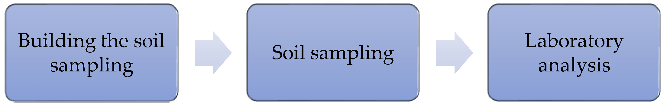
Figure 2.
Stages of the Digital Soil Cube (DSC) method.
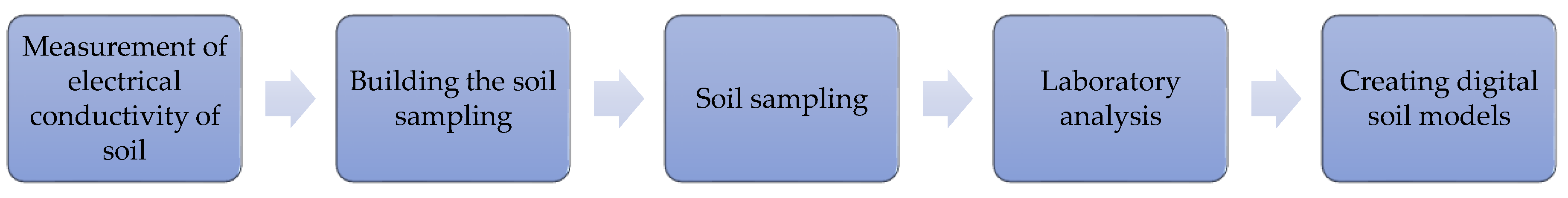
Figure 3.
Top Soil Mapper (Geoprospectors GmbH).
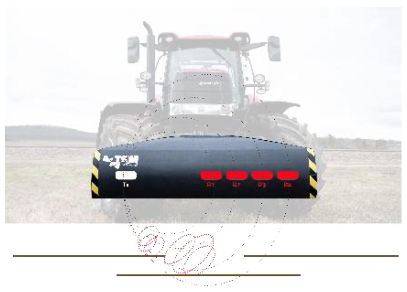
Figure 4.
Zones and field markers (from TSM Client Cloud & Skanfield-5S) *; *- full field coordinates not presented.
Figure 4.
Zones and field markers (from TSM Client Cloud & Skanfield-5S) *; *- full field coordinates not presented.

Table 1.
Rating scale.
| Parameters |
С mg/kg |
N mg/kg |
P mg/kg |
C/ N |
|---|---|---|---|---|
| Very low | < 50 | <0,98 | < 398 | < 8 |
| Low | 50 -100 | 98-133 | 398 - 553 | 8 -10 |
| Average | 100 -150 | 133-195 | 553 - 924 | 10-12 |
| High | 150 -250 | 195-286 | 924 - 1599 | >12 |
| Very high | > 250 | >286 | >1599 | > 30 |
Disclaimer/Publisher’s Note: The statements, opinions and data contained in all publications are solely those of the individual author(s) and contributor(s) and not of MDPI and/or the editor(s). MDPI and/or the editor(s) disclaim responsibility for any injury to people or property resulting from any ideas, methods, instructions or products referred to in the content. |
© 2024 by the authors. Licensee MDPI, Basel, Switzerland. This article is an open access article distributed under the terms and conditions of the Creative Commons Attribution (CC BY) license (http://creativecommons.org/licenses/by/4.0/).
Copyright: This open access article is published under a Creative Commons CC BY 4.0 license, which permit the free download, distribution, and reuse, provided that the author and preprint are cited in any reuse.


