
Submitted:
07 December 2024
Posted:
09 December 2024
You are already at the latest version
Abstract
In this study, we introduce generalized k-order Fibonacci and Lucas (F&L) polynomials that allow the derivation of well-known polynomial and integer sequences such as the sequences of k-order Pell polynomials, k-order Jacobsthal polynomials, k-order Jacobsthal F&L numbers. Within the scope of this research, a generalization of hybrid polynomials is given by moving them to the kth order. Hybrid polynomials defined by this generalization are called as k-order F&L hybrinomials. A key aspect of our research is the establishment of the recurrence relations for generalized k-order F&L hybrinomials. After we give the recurrence relations for these hybrinomials, we obtain the generating functions of hybrinomials shedding light on some of their important properties. Finally, we introduce the matrix representations of the generalized k-order F&L hybrinomials and give some properties about the matrix representations.
Keywords:
Fibonacci polynomials
; generalized order Fibonacci and Lucas polynomials
; hybrid numbers
; hybrid polynomials
; generalized order Fibonacci
; Lucas hybrinomials
MSC: 11B39; 11R52; 05A15; 15A63; 15A66
1. Introduction
F&L numbers, which have the most interesting properties and relationships in the world of the mathematics, have been found interesting by many authors. Fibonacci numbers are defined by the recurrence relation of , with initial conditions for . With a similar definition, the recurrence relation of Lucas numbers can be given as for with the initial condition of . (for more details see [1,2,3]). One of the most important and popular features of the Fibonacci sequence is its matrix representation so-called Fibonacci -matrix in [4] as follows:
Also, -power of the Fibonacci -matrix is shown in [5] by
Fibonacci polynomials were first studied in 1883 by Belgian mathematician E. Charles Catalan and German mathematician E. Jacobsthal. The Fibonacci polynomials studied by Catalan were later developed by M. N. Swamy in 1966. In addition, a new Fibonacci type polynomial was added to the literature by P. F. Bryd in 1963. The polynomial defined by P. F. Bryd is today called the Pell polynomial. The polynomial accepted as the Fibonacci polynomial is the polynomial defined by Catalan. Later, all these different definitions were named as F&L type polynomials.
The recurrence relation of Fibonacci polynomials defined by Catalan is defined as follows:
where for . It can be easily seen that , where is the Fibonacci number.
Generalized k-order F&L numbers that were introduced in [6] are defined by the following recurrence relation for integers ;
with initial conditions .
The concept of the hybrid numbers and polynomials is a field gaining increasing prominence in mathematics, physics and engineering. Hybrid numbers are a generalization of complex, hyperbolic and dual numbers. Until today, many authors have studied on these numbers. Ulrych in 2005 in [22] explored the potential of hyperbolic numbers in relativistic quantum physics, demonstrating their use as a generalization of complex numbers within this framework. This work highlights the potential for hybrid numbers to offer new perspectives and tools for understanding quantum phenomena. Also, Branicky in 1998 in [23] provided a significant contribution to the analysis of hybrid systems by introducing multiple Lyapunov functions as a tool for stability analysis, expanding the available techniques for understanding these complex systems. The non-commutative number system including these three number systems were defined in [7]. The set of hybrid numbers is defined as
Let and be any two hybrid numbers. The operation of equality, addition, subtraction and multiplication by scalar are defined as follows:
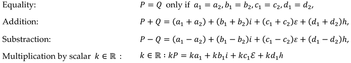
The multiplication of hybrid numbers is defined in the following table using Eq. (1) as:
Horadam hybrid numbers were introduced in [8] for the first time. Later, in [9], Fibonacci hybrid numbers were studied and some important properties about the hybrid numbers were presented. (for a more details of these numbers, see also [10,11,12]). Besides these, Jacobsthal, Jacobsthal-Lucas hybrid numbers and the Pell, Pell-Lucas hybrid numbers were introduced in [13,14] by using the terms of these sequences. More information regarding these sequences can be found in [15,16,17,18]. A new generalization based on these studies was defined in [19]. Also, some algebraic properties regarding F&L hybrid numbers were given in it. In [6], these studies were generalized and generalized k-order F&L hybrid numbers were defined. Furthermore, in the same study matrix representations of generalized k-order F&L hybrid numbers were described by using Table 1. In their work titled "Recurrence relations for the sections of the generating series of the solution to the multidimensional difference equation", Akhtamova in [21] investigated recurrence relations for the sections of the generating series of the solution to the multidimensional difference equation.
In this study, we define generalized k-order F&L polynomials, that is a generalization of the generalized k-order F&L numbers. We also obtain similar generalization for hybrid numbers as well. Finally, we define the matrix representations for generalized k-order F&L hybrinomials and give some properties about the matrix representations.
2. Generalized k-Order F&L Polynomials
In this section, we define generalized k-order F&L polynomials. Then, we give some special cases of generalized k-order F&L polynomials such as Fibonacci polynomials, Lucas polynomials, Pell polynomials, Pell-Lucas polynomials and many special polynomials.
Definition 2.1. For , the generalized k-order F&L polynomials are defined by the following recurrence relations
with initial conditions for
Some special cases of generalized -order F&L polynomials are in Table 2 as follows:
1. For ; we get the following table:
2. For and ; we get Tribonacci polynomials. The recurrence relation of Tribonacci polynomials is
with the boundary conditions .
3. For and , we get -order Fibonacci polynomials.
4. For and , we get -order Lucas polynomials.
5. For and , we get -order Pell polynomials.
6. For and , we get -order Pell-Lucas polynomials.
7. For and , we get -order Jacobsthal polynomials.
8. For and , we get -order Jacobsthal-Lucas polynomials.
It is easy to see that generalized -order F&L numbers are obtained by selecting specifically as shown in [4].
3. Generalized k-Order Fibonacci and Lucas Hybrinomials
In this section, we define hybrinomials using generalized -order F&L polynomials. We describe the recurrence relation of hybrinomials, generating functions and give some special results.
Definition 3.1. The generalized -order F&L hybrinomials are defined a
where is generalized -order F&L polynomials.
Some special cases of the generalized -order F&L hybrinomials are as follows:
1. For , we obtain some special hybrinomials using (2) in Table 3 as follows:
2. For and , we get Tribonacci hybrinomials.
Definition 3.2. For every , the conjugate of is defined by
.
Theorem 3.1. For every , we have the following properties:
- i.
- where is the generalized -order F&L polynomials.
- ii.
- iii.
- where and
Proof.
- i.
- The proof is easily seen using the definitions of and .
- ii.
- Using , and the multiplication of hybrid numbers, we obtain as follows:
- iii.
- First, we obtain as follows:
Then, we use (ii). From (ii), we have
This we obtain as follows:
Theorem 3.2. The recurrence relation of the generalized -order F&L hybrinomials is defined as follows:
with the initial conditions
Proof. It can be proved by using (2) and (3).
In the following theorem, we give some relations between and for every .
Theorem 3.3. The generating function for the generalized -order F&L hybrinomials is
Proof. Let be the generating function for the generalized -order F&L hybrinomials. By making some algebraic operations, we get the following formula:
Then, we make the necessary arrangements. Thus, we obtain
Corollary 3.1. For , we obtain the generating function of the generalized -order F&L hybrid numbers in [4] as follows:
where is the generalized order F&L hybrid number.
Corollary 3.2. For ; we get the generating function of Horadam hybrinomials in [19] as follows:
Corollary 3.3. For the case of , we get the generating functions of the following hybrinomials depending on the choice of and as follows:
Corollary 3.4. For and , we obtain the generating functions of the Horadam, Fibonacci, Lucas, Pell, Pell-Lucas, Jacobsthal and Jacobsthal-Lucas hybrid numbers.
4. Matrix Representations of the Generalized k-Order Fibonacci and Lucas Hybrinomials
In this section, we define matrix representations of generalized -order F&L hybrinomials. First, we derive matrices and that play similar role to the -matrix of Fibonacci numbers.
We determine matrices and as follows:
and
Lemma 4.1. Let and be matrices that is defined with the above equalities. Then, we get
for .
Proof. By multiplying matrices and , we get a matrix as following:
According to the matrix multiplication,
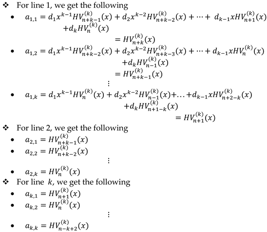
All the other elements of the other rows are found in the same way.
Since
we get .
Theorem 4.1. Let and be matrices that is defined as above. Then,
for .
Proof. This theorem is proved by induction on . It is easily seen that the assertion is true for since
Assuming the assertion is true for , we have
By multiplying each side of this equality with , we get
Using Lemma 4.1, we obtain
Thus, the proof is completed.
Corollary 4.1. For , we get the matrix representation of generalized -order F&L hybrid numbers that is shown in [4].
Corollary 4.2. For , we can show the matrix representation of Horadam hybrinomials in [12] as
Corollary 4.3. For , we can get some special matrix representations as follows:
- For and , Fibonacci hybrinomials,
- For and , Lucas hybrinomials,
- For and , Pell hybrinomials,
- For and , Pell-Lucas hybrinomials.
- For and , Jacobsthal hybrinomials,
- For and , Jacobsthal-Lucas hybrinomials.
Corollary 4.4. For , and , we can show the matrix representation of Tribonacci hybrinomials as follows:
Also, when we take in this notation, we get the matrix representation of Tribonacci hybrid numbers.
Corollary 4.5. For and , we get the matrix representations of the Horadam, Fibonacci, Lucas, Pell, Pell-Lucas, Jacobsthal and Jacobsthal-Lucas hybrid numbers.
Corollary 4.6. Let for . Then we get as
5. Conclusions
This study consists of four parts. In the first part of this study, Fibonacci numbers, Fibonacci polynomials and previous studies about the topic that we consider in this article were mentioned. In addition, the definition of hybrid numbers was made and the multiplication table was given.
In the second part of this study, we defined the generalized -order F&L polynomials by using the generalized -order F&L numbers that we have defined earlier. For the special cases of and , we show that one can obtain Horadam, Fibonacci, Pell, Pell-Lucas, Jacobsthal, Jacobsthal-Lucas numbers and their polynomials. By changing these selections, we can obtain other special polynomials and numbers.
In the third part of this study, we defined the generalized -order F&L hybrinomials using the generalized -order F&L polynomials. Besides, we described the recurrence relations of the generalized -order F&L hybrinomials. With special choices in this recurrence relation, one can obtain the hybrid polynomials such as Horadam, Fibonacci, Lucas, Pell, Pell-Lucas, Jacobsthal, Jacobsthal-Lucas hybrinomials. Also, we introduced the generating functions of hybrinomials and gave some important properties of hybrinomials.
The last part of this study, we gave matrix representations of the generalized -order F&L hybrinomials. We show that by special choices of the integers and , one can obtain matrix representations of some known hybrid polynomials such as Horadam, Fibonacci, Lucas, Pell, Pell-Lucas, Jacobsthal and Jacobsthal-Lucas hybrinomials.
As a result, by changing the integers and that we is used in these definitions, we can define many known special polynomials and hybrinomials such as Balancing, Chebyshev hybrinomials etc.
Author Contributions
Conceptualization, S.A. and G.K-G.; methodology, S.A. and G.K-G.; validation, S.A. and G.K-G.; formal analysis, S.A. and G.K-G.; investigation, S.A. and G.K-G.; resources, S.A. and G.K-G.; writing—original draft preparation, S.A. and G.K-G.; writing—review and editing, S.A. and G.K-G.; visualization, S.A. and G.K-G.; supervision, G.K-G. All authors have read and agreed to the published version of the manuscript.
Funding
This research received no external funding.
Data Availability Statement
Data are contained within the article.
Conflicts of Interest
The authors declare no conflicts of interest.
References
- Altassan, A.; Alan, M. On mixed concatenations of Fibonacci and Lucas numbers which are Fibonacci numbers. Math. Slovaca 2022, 74, 563–576. [Google Scholar] [CrossRef]
- Koshy, T. Fibonacci and Lucas numbers with applications, 2nd ed.; John Wiley: New York, 2018. [Google Scholar]
- Vajda, S. Fibonacci and Lucas Numbers and the Golden Section: Theory and Applications, Ellis Harwood Limited: England, 1969. [CrossRef]
- Gould, H. W. A history of the Fibonacci Q-matrix and a higher-dimensional problem. The Fibonacci Quart. 1981; 19, 250-257. [CrossRef]
- Stakhov, A. P. A generalization of the Q-matrix. Reports of the National Academy of Sciences of Ukraine 1999; 9, 46-49.
- Asci, M.; Aydinyuz, S. Generalized order Fibonacci and Lucas hybrid numbers. J. Inf. Optim. Sci. 2021, 42, 1765–1782. [Google Scholar] [CrossRef]
- Özdemir, M. Introduction to hybrid numbers. Adv. Appl. Clifford Algebr. 2018, 28. [Google Scholar] [CrossRef]
- Szynal-Liana, A. The Horadam hybrid numbers. Discuss. Math. Gen. Algebra Appl. 2018, 38, 91–98. [Google Scholar] [CrossRef]
- Szynal-Liana, A.; Wloch, I. The Fibonacci hybrid numbers. Util. Math. 2019, 110, 3–10. [Google Scholar]
- Kızılateş, C. A note on Horadam hybrinomials. Fundam. J. Math. Appl. 2022, 5, 1–9. [Google Scholar] [CrossRef]
- Özkoç, A. Binomial Transforms for Hybrid Numbers Defined Through Fibonacci and Lucas Number Components. Konuralp J. Math. 2022, 10, 282–292. [Google Scholar]
- Szynal-Liana, A.; Wloch, I. Introduction to Fibonacci and Lucas hybrinomials. Complex Var. Elliptic Equ. 2020, 65, 1736–1747. [Google Scholar] [CrossRef]
- Szynal-Liana, A.; Wloch, I. On Jacobsthal and Jacobsthal-Lucas hybrid numbers. Ann. Math. Sil. 2019, 33, 276–283. [Google Scholar] [CrossRef]
- Liana, M.; Szynal-Liana, A.; Wloch, I. On Pell hybrinomials. Miscolc Math. Notes 2019, 20, 1051–1062. [Google Scholar] [CrossRef]
- Bród, D.; Michalski, A. On Generalized Jacobsthal and Jacobsthal–Lucas Numbers. Ann. Math. Sil. 2022, 36, 115–128. [Google Scholar] [CrossRef]
- Ganie, A.H.; AlBaidani, M.M. Matrix Structure of Jacobsthal Numbers. J. Funct. Spaces 2021; Article ID: 2888840. [CrossRef]
- Gong, Y.; Jiang, Z.; Gao, Y. On Jacobsthal and Jacobsthal-Lucas Circulant Type Matrices. Abstr. Appl. Anal. 2015, Article ID 418293. [CrossRef]
- Karadeniz Gözeri, G. On Pell, Pell-Lucas, and balancing numbers. J. Inequal Appl. 2018; 3. [CrossRef]
- Kızılateş, C. A new generalization of Fibonacci hybrid and Lucas hybrid numbers. Chaos Solitons Fractals 2020, 130, 1–5. [Google Scholar] [CrossRef]
- Cerda Moreles, G. Introduction to third-order Jacobsthal and modified third-order Jacobsthal hybrinomials. Discuss. Math. Gen. Algebra Appl. 2021, 41, 139–152. [Google Scholar] [CrossRef]
- Lyapin, A.; Akhtamova, S.S. Recurrence relations for the sections of the generating series of the solution to the multidimensional difference equation. Vestn. Udmurtsk. Univ. Mat. Mekh. Komp. Nauki 2021, 31, 414–423. [Google Scholar] [CrossRef]
- Ulrych, S. Relativistic quantum physics with hyperbolic numbers. Physics Letters 2005; 625, 313-323. [CrossRef]
- Branicky, M. Multiple Lyapunov Functions and Other Analysis Tools for Switched and Hybrid Systems. IEEE Trans. Autom. Control. 1998, 43. [Google Scholar] [CrossRef]

Table 1.
The multiplication of hybrid numbers.
Table 2.
Special polynomials.
| Special Polynomials | |||
| 1 | 1 | 2 | Lucas polynomials |
| 2 | 1 | 1 | Pell polynomials |
| 2 | 1 | 2 | Pell-Lucas polynomials |
| 1 | 2 | 1 | Jacobsthal polynomials |
| 1 | 2 | 2 | Jacobsthal-Lucas polynomials |
Table 3.
Special Hybrinomials.
| Special Polynomials | |||
| - | - | - | Horadam hybrinomials in [12] |
| 1 | 1 | Fibonacci hybrinomials in [12] | |
| 1 | 1 | 2 | Lucas hybrinomials in [12] |
| 2 | 1 | 1 | Pell hybrinomials in [12] |
| 2 | 1 | 2 | Pell-Lucas hybrinomials in [12] |
| 1 | 2 | 1 | Jacobsthal hybrinomials in [12] |
| 1 | 2 | 2 | Jacobsthal-Lucas hybrinomials in [12] |
Disclaimer/Publisher’s Note: The statements, opinions and data contained in all publications are solely those of the individual author(s) and contributor(s) and not of MDPI and/or the editor(s). MDPI and/or the editor(s) disclaim responsibility for any injury to people or property resulting from any ideas, methods, instructions or products referred to in the content. |
© 2024 by the authors. Licensee MDPI, Basel, Switzerland. This article is an open access article distributed under the terms and conditions of the Creative Commons Attribution (CC BY) license (http://creativecommons.org/licenses/by/4.0/).
Copyright: This open access article is published under a Creative Commons CC BY 4.0 license, which permit the free download, distribution, and reuse, provided that the author and preprint are cited in any reuse.


