Preprint
Article

This version is not peer-reviewed.

Understanding Congestion Risk and Emissions of Various Travel Behavior Patterns Based on License Plate Recognition Data

A peer-reviewed article of this preprint also exists.

Submitted:

04 December 2024

Posted:

05 December 2024

You are already at the latest version

Abstract

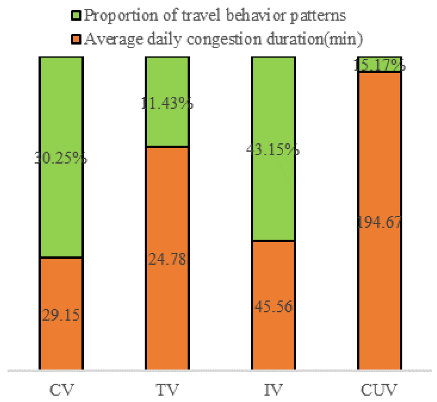
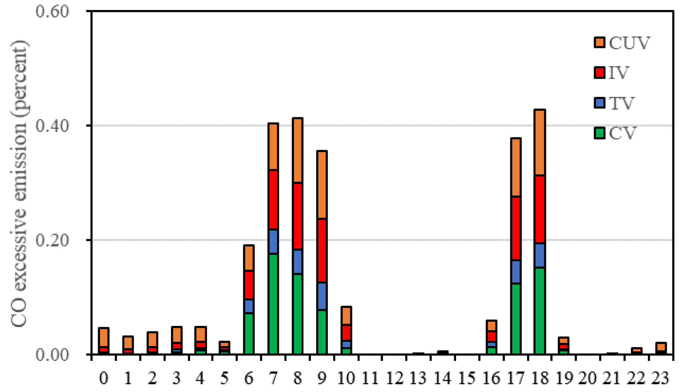
Understanding vehicle travel behavior patterns is essential for managing urban traffic congestion, as well as for addressing the associated congestion risks and excess emissions. This study, based on one week of License Plate Recognition (LPR) data from urban expressway networks, investigates different travel behavior patterns and their related congestion risks and emissions. First, we classify vehicles into distinct travel patterns based on spatiotemporal features extracted from LPR data and propose a scalable pattern recognition method suitable for large-scale applications. We then assess the congestion risks associated with each pattern and estimate the excess emissions resulting from congestion. The results reveal substantial variation in congestion risks across different travel patterns, with congestion risks following a bimodal distribution, influenced by temporal traffic flow rhythms. Furthermore, the excess emissions from congestion caused by commercially used vehicles (CUVs) are comparable to those of individually owned vehicles (IVs), despite CUVs constituting only one-third of the total vehicle count. This suggests that focusing solely on commuter travel modes underestimates both congestion risks and excess emissions.

Keywords: 
;  ;  ;  ;  

1. Introduction

Traffic congestion has long been a global issue, leading not only to time losses and economic setbacks [1,2], but also posing significant risks to individuals' physical and mental well-being [3,4]. In an effort to alleviate congestion, administrators promote changes in travel behavior [5]. The success of these management strategies largely depends on understanding travelers' behavior patterns and the congestion risks associated with each pattern [6]. For instance, when planning travel routes, it is crucial to account for commuters' preference for fixed paths. Ineffective route recommendations can result in confusion and inconvenience for travelers. Moreover, those facing higher congestion risks may be more open to adjusting their travel times or routes. Therefore, gaining insights into travelers' behavior patterns and the corresponding congestion risks is vital for formulating effective management policies.
Research on travel behavior has traditionally relied on data-driven methods [7,8]. With advancements in information technology, an increasing variety of data sources has been incorporated into such studies [9], including License Plate Recognition (LPR) data, mobile signaling data, questionnaire/telephone survey data, and bus card data. In the early stages, travel behavior research predominantly utilized travel survey data collected through paper questionnaires, telephone interviews, and online surveys. Using these data, researchers explored various aspects, such as commuters' travel time preferences [10], travel mode selection [11], and more complex patterns of travel behavior [12]. However, the high cost of collecting survey data limits both sample size and frequency [13], rendering traditional surveys inadequate for comprehensive studies of travel behavior patterns. Consequently, some researchers have turned to mobile signaling data, which have been used to investigate travel patterns and population distribution [14], infer individual attributes and activity types [15], analyze personal mobility trajectories [16], and mine travel purposes [17]. Despite these applications, mobile phone data pose challenges in accurately inferring individual travel behavior patterns, as they cannot differentiate between transportation modes such as subway, private car, taxi, or bicycle. Similarly, data from bus card transactions fail to provide a holistic representation of overall travel patterns [18].
LPR data offers more comprehensive coverage, enabling the collection of information from all vehicles on the road network and facilitating the extraction of detailed insights into vehicle travel time and spatial activities. As a result, multi-day vehicle trajectory data derived from LPR presents new opportunities for in-depth studies on travel behavior patterns. For example, [19] explored the impact of two different vehicle restriction policies on traffic conditions, finding that these restrictions led to more "illegal" travel and increased travel intensity. [20] examined the effects of vehicle traffic restrictions on the behavior of non-Shanghai licensed vehicles, analyzing their travel patterns. [21] proposed a method to assess travel behavior regularity based on the order of travel or activity organization, categorizing travel behavior patterns into conventional and unconventional types. Sun et al. [22] used LPR data to identify both regular and abnormal patterns in individual travel behavior. However, the distinction between conventional and unconventional patterns is insufficient to support sophisticated demand management strategies. [23] developed multiple indicators to represent commuting patterns by utilizing vehicle travel OD information, extracting commuting rules through clustering and decision tree algorithms. [24] also leveraged LPR data from Cambridge, UK, to study the non-commuting travel demand of commuters. [5] proposed a systematic method for identifying travel behaviors and purposes based on weekly trajectory data from 6600 trams in Shanghai. Using a Gaussian mixture model, they categorized vehicle travel behavior into four groups, including commuting. However, the algorithm's complexity limits its application to large-scale road networks. LPR data addresses challenges such as small sample sizes, low data quality, and difficulty in obtaining survey-based data. Research on travel behavior patterns based on LPR data has become a key element in the theoretical framework of human mobility, though its data advantages have yet to be fully exploited. Most studies focus on OD points and tend to analyze a single travel mode, overlooking travel path preferences, time preferences, travel distances, and other critical factors. Furthermore, the design of travel behavior pattern indicators needs further optimization. Current research often relies on empirically derived parameters and indicators, rather than mining travel behavior patterns directly from the data.
Existing research on traffic congestion risks has primarily focused on commuting patterns, with limited exploration of other travel behaviors [25,26]. For example, [27] examined how traffic congestion impacts individual commuting satisfaction [28]explored differences in perceived congestion satisfaction among individuals using various modes of transportation for commuting. Given the higher congestion risks associated with commuting, [29] proposed staggered working hours as an effective strategy to alleviate peak congestion. However, the feasibility and sustainability of such policies remain debated. In reality, road networks accommodate a variety of travel patterns [30], and focusing solely on commuting may lead to an underestimation of overall congestion risks. Therefore, congestion mitigation strategies should address a broader range of travel behaviors, rather than concentrating on a single mode of transportation.
Based on the background described above, this paper first preprocesses and generates trajectories from one week of LPR data collected on the expressway network of a city in China. It then constructs multiple novel spatiotemporal features and applies three different clustering methods to classify vehicle categories. Subsequently, a pattern recognition model is developed using LightGBM. The congestion risks and excess emissions associated with each pattern are analyzed, followed by recommendations for congestion management strategies. The contributions of this paper are as follows:
  • A novel method for dividing travel behavior patterns based on a unique set of spatiotemporal feature indicators is proposed. This method uses clustering to identify homogeneous clusters from data features, overcoming the subjectivity and limitations of traditional threshold-based approaches.
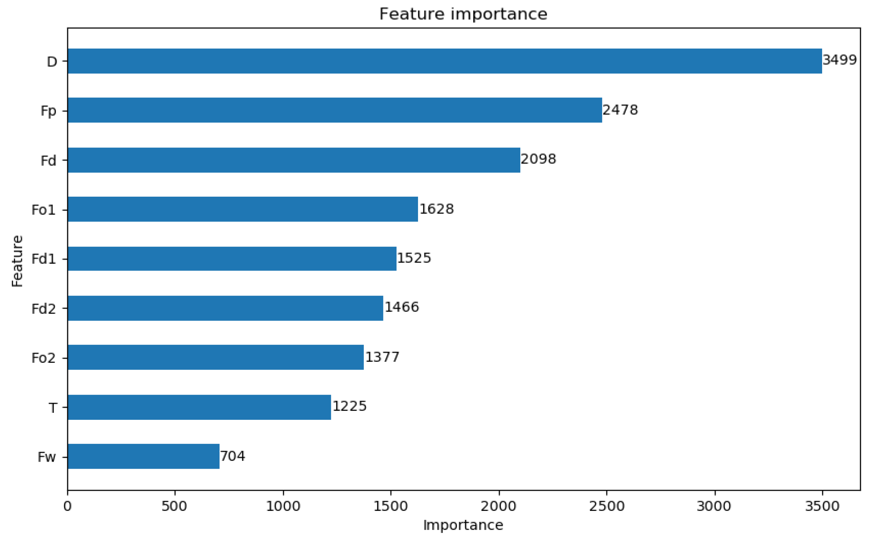
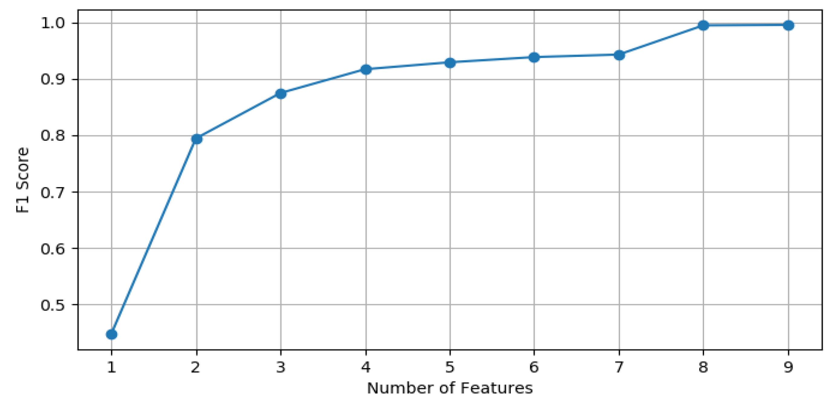
  • A pattern recognition method suitable for large-scale applications is presented, demonstrating strong recognition performance with only three feature values.
  • The congestion risks and excess emissions of various travel patterns are analyzed based on real-world LPR data. The findings offer important insights for individual travel time planning and health management, and provide support for the development of personalized, proactive traffic demand management measures.
The remaining sections of this paper are organized as follows: Section 2 introduces the data sources, pattern recognition methods, and the estimation methods for congestion risks and excess emissions. Section 3 presents the experimental results based on real-world LPR data. Section 4 discusses the congestion risks of each pattern and proposes strategies for congestion mitigation. Finally, Section 5 concludes the study.2 Methodology
The congestion risk estimation method for various travel behavior patterns proposed in this paper is illustrated in 0. The study is structured into three key components: (1) the construction of spatiotemporal characteristic indices for travel behavior, (2) the classification and recognition of travel behavior patterns, and (3) the estimation of congestion risk. Each of these components is described in detail in the following sections.
Figure 1. Research Framework.
Preprints 141852 g001

2.1. Study Area and Data

The data used in this study consists of LPR data recorded from vehicles passing through an expressway in a Chinese city during a one-week period in 2022. The study area is shown in 0. The road network is equipped with tens of thousands of LPR detectors. The data collected by these detectors is divided into two components: the first part contains information about the LPR detectors themselves, while the second part provides details on the passing vehicles, as outlined in 0 and 2.
Figure 2. Expressway network structure.
Preprints 141852 g002
Table 1. Information of the LPR detectors.
Name Information Explanation
CardID 442311111111111111 Serial number of the detector
PlaceCode 50122 Serial number of detector’s location
Latitude 39.921111 Information of latitude
Longitude 116.461111 Information of longitude
Table 2. Information of passing cars.
Name Information Explanation
MotorVehicleID 114211111111111111 Serial number of the record
PlateNo Yue B.XXXXX License plate number
PlateColor 02 Type of car
PassTime 2022-08-05 02:29:30 Time of record
Roadclid 7285 Serial number of the road segment
CardID 442311111111111111 Serial number of the detector
Through statistical analysis, this study collected 156,723,515 vehicle flow records, which contained quality issues such as missing license plates, duplicate detections, and erroneous values. Specifically, missing license plates accounted for 0.02%, duplicate detections for 0.33%, and erroneous data for 4.11%. The total amount of problematic data did not exceed 5%, and its overall impact was minimal, so this data was excluded from the analysis.
The road network detection equipment is dense, evenly distributed, and individual road segments do not exceed 3 km in length. Vehicle trajectories were generated sequentially based on chronological order and the upstream-downstream relationships within the road network topology. Following [31], detections of vehicles with intervals of less than one hour were considered part of the same trip, enabling the identification of individual travel trips. After processing, a total of 1,144,105 vehicles and 10,389,842 travel trajectories were generated.

2.2. Identification of Travel Behavior Patterns

2.2.1. Construction of Spatiotemporal Feature Indicators

Daily travel patterns are influenced by activity demands, with each trip linked to specific spatiotemporal activities at the destination, which in turn shape the characteristics of the trip and the associated travel behavior patterns. Understanding these patterns is essential for effective traffic demand management, urban planning, and resource allocation [18]. In this study, nine indicators were developed using LPR data to capture the spatiotemporal features of travel behavior comprehensively. By analyzing vehicle trajectory data across the road network, the study evaluated the stability of vehicle travel and the frequency of daily trips, offering valuable insights into travel activity levels.
The weekday travel stability coefficient F w is defined as follows.
F w = n w N  
where N represents the total number of weekdays surveyed, and n w ​ denotes the number of days a particular vehicle was detected.
The daily travel frequency F d is defined as follows.
F d = n d N
where n d represents the total number of trips made by a specific vehicle within the statistical scope.
Access frequency is a key component in the theory framework of human mobility, representing the number of times an individual visits a certain location within a unit of time [32]. Building upon this notion, this study extracts the initial and final travel trajectories of individual vehicles on a daily basis using LRP data, characterizing the spatial stability of travel behavior through the access frequency of these start and end points. Assuming that within the study timeframe, the starting points of vehicles' first and last daily trips are denoted as O 1 and O 2 respectively, and the corresponding end points as D 1 and D 2 .
The weekday initial trip origin stability coefficient F O 1 is defined as follows.
F O 1 = m a x ( f O 1 , f O 2 , , f O n ) n w
Where max m a x ( f O n ) represents the number of times the highest frequency origin point appears for a vehicle's first trip during weekdays.
The weekday last-trip origin point stability coefficient F O 2 is defined as follows.
F O 2 = m a x ( l O 1 , l O 2 , , l O n ) n w
where m a x ( l O n ) denotes the number of times the highest frequency origin point appears for a vehicle's last trip during weekdays.
The weekday first-trip destination point stability coefficient F D 1 is defined as follows.
F D 1 = m a x ( f D 1 , f D 2 , , f D n ) n w
Where m a x ( f D n ) represents the number of times the highest frequency destination point appears for a vehicle's first trip during weekdays.
The weekday last-trip destination point stability coefficient F D 1 is defined as follows.
F D 1 = m a x ( l D 1 , l D 2 , , l D n ) n w
where m a x ( l D n ) denotes the number of times the highest frequency destination point appears for a vehicle's last trip during weekdays.
In addition to the frequency of visits to origin and destination points, path similarity can also characterize the spatial stability of travel behavior. The difference lies in that path similarity focuses on the overall frequency of traversed paths and can also reflect the vehicle's path preferences. This study calculates path similarity based on the Jaccard coefficient.
The travel path similarity F P is defined as follows.
F P = P 1 P 2 P n w P 1 + P 2 + + P n w P 1 P 1 P n w
Where P n w represents the set of road segments for a particular travel path.
Considering the extraction of comprehensive spatiotemporal features from massive LPR data, this study utilizes the average daily travel distance to characterize the spatial features of travel behavior.
The average daily travel distance D is defined as follows.
D = i = 1 n d D i 100 N
Where D i represents the distance traveled by a vehicle in a single trip, in kilometers.
Regarding the temporal features of travel behavior, existing studies often use travel periods for characterization. For instance, [23] identify commuting patterns based on travel during morning and evening peak periods. However, regardless of commuting or other travel patterns, they may not necessarily be concentrated during these peak periods. Therefore, considering that travel times can be obtained from LPR data, this study utilizes the standard deviation of the time of the first trip on workdays to characterize the temporal features of travel behavior, while also reflecting the sensitivity of travelers to time constraints.
The travel time stability coefficient T is defined as follows:
T = 1 , 0 , σ 30 σ > 30   ,   σ = i = 1 n ( t i t ¯ ) 2 n
Where t i represents the time of the first trip on a workday for a vehicle, t ¯ represents the average time of the first trip on a workday for a vehicle. After statistical analysis, when the standard deviation of the time of the first trip on workdays within the study road network is 30 minutes, this grouping has the largest proportion. Therefore, σ is set to 30.

2.2.2. Classification of Travel Behavior Patterns

Based on the aforementioned spatio-temporal feature indicators, we aim to reduce the dimensionality of each feature variable to eliminate correlations, summarize existing observed variables with fewer latent variables, and improve clustering algorithm efficiency. To address the uneven distribution of feature data, we apply various clustering algorithms for pattern classification and compare their performance to select the optimal algorithm. The process is as follows:
(1) Dimensionality Reduction: Before reducing the dimensionality of each feature, we first conduct KMO and Bartlett tests to evaluate the suitability of the data structure for dimensionality reduction. Next, we determine the number of principal components based on the Kaiser criterion, scree plot, and variance explanation criterion [33], and then perform dimensionality reduction.
(2) Determination of the Optimal Number of Clusters: After dimensionality reduction, we determine the optimal number of clusters to partition travel behavior patterns, typically using the elbow method. The core idea behind the elbow method is as follows: when the number of clusters, k , is smaller than the actual number of clusters, increasing k significantly enhances intra-cluster cohesion, which leads to a large decrease in the within-cluster sum of squares (Inertia). However, as k approaches the true number of clusters, further increases in k result in diminishing returns, and the rate of decrease in Inertia flattens out. This relationship between Inertia and k forms an elbow shape, where the "elbow point" indicates the optimal number of clusters. The formula for calculating the within-cluster sum of squares is shown below.
I n e r t i a = p C i p m i 2
Where C i represents the i cluster, p is a sample point in cluster C i , and m i is the centroid of the cluster.
(3) Clustering. After determining the optimal number of clusters, we apply three clustering algorithms—K-means, Agglomerative Clustering, and DBSCAN—to analyze the dataset. The K-means algorithm partitions the data into K clusters, ensuring high similarity among data points within each cluster. Agglomerative Clustering, a distance-based hierarchical method, iteratively merges data points into clusters, minimizing internal distances and maximizing external distances. DBSCAN, a density-based algorithm, forms clusters by identifying regions of high data point density. These three methods are employed to uncover distinct travel behavior patterns across all vehicles. The clustering results are evaluated using the silhouette coefficient, as defined in Equation (11).
S = b a m a x ( a , b )
Here, a   represents the average distance between sample x i and other samples within the same cluster, referred to as cohesion, while b denotes the average distance between x i and all samples in the nearest cluster, known as separation. The silhouette coefficient ranges from −1 to 1, with values closer to 1 indicating better clustering performance. A value less than zero indicates poor clustering performance, with many points misclassified.

2.2.3. Travel Behavior Pattern Recognition

After partitioning patterns based on historical LPR data, an efficient classifier must be constructed to recognize patterns among a large number of vehicles, including newly added ones. To achieve this, we employ the LightGBM (Light Gradient Boosting Machine) algorithm, which is capable of efficiently processing large datasets. LightGBM is an ensemble method based on gradient boosting, and one of its key innovations is the Gradient-based One-Side Sampling (GOSS) algorithm. GOSS selectively retains instances with larger gradients while randomly sampling instances with smaller gradients. Specifically, the GOSS algorithm first sorts instances by the absolute values of their gradients and selects the top "a" instances. Then, it randomly samples "b" instances from the remaining data. In the process of calculating information gain, the algorithm multiplies the gradients of the sampled instances with smaller gradients by (1-a)/b. This strategy enables the algorithm to focus more on underrepresented instances while maintaining the overall distribution of the original dataset. Let O represent the training dataset at a fixed node of the decision tree. The variance gain of splitting feature j at point d for this node is defined as
V j O ( d ) = 1 n O ( ( x i O : x i j d g i ) 2 n l O j ( d ) + ( x i O : x i j > d g i ) 2 n r O j ( d ) )
where n O = I x i O n l O j d = I x i O : x i d , n r O j ( d ) = I x i O : x i > d .
The formula for calculating the estimated variance gain V ~ j d of the GOSS algorithm is as
V ~ j ( d ) = 1 n ( ( x i A : x i j d g i + 1 a b x i B : x i j d g i ) 2 n l j ( d ) + ( x i A : x i j > d g i + 1 a b x i B : x i j > d g i ) 2 n r j ( d ) )
A   represents the subset with larger gradients and B represents the subset with smaller gradients. And 1 a b is used to normalize the sum of the gradients over B.
Furthermore, the exclusive feature bundling algorithm can combine many exclusive features into fewer dense features, effectively avoiding unnecessary computation for zero feature values.
In this study, the data samples are divided in a ratio of 0.8:0.2, with 80% of the dataset utilized for training the proposed model and 20% for testing the trained model. Additionally, the F1-score is selected as the measurement method for the classification model in this paper. The F1-score considers both precision and recall, providing a balanced assessment of the model's accuracy between precision and recall.

2.3. Estimation of Congestion Risk and Excessive Emissions

Based on the aforementioned division of travel patterns, we measure congestion risk by calculating the actual travel time and the ideal travel time for each trip trajectory. The expression for the ideal travel time is given by:
t ( 1 , m ) i = j = 1 n 1 L j v ^ j
Where t ( 1 , m ) i represents the ideal travel time for vehicle i in the m th trip, L j denotes the length of segment   j , v ^ j represents the speed of segment j under free-flow conditions, and   n 1 denotes the total number of segments for vehicle i in the j th trip.
The expression for the actual travel time is given by:
t ( 2 , m ) i = t ( e n d , m ) i t ( s t a r t , m ) i
Where t ( 2 , m ) i represents the actual travel time for vehicle i in the m th trip, t ( s t a r t , m ) i and t ( e n d , m ) i respectively represent the start and end times of the trip for vehicle   i , obtained from LPR data.
Therefore, the expression for the congestion exposure time corresponding to the k th travel pattern is:
T k = 1 n 2 1 m ( t ( 2 , m ) i r t 1 , m i ) m n 2
Where T represents the congestion exposure time for a single trip of vehicle data corresponding to the k th travel pattern, r represents the preset congestion coefficient [34], taken as 1.5 in this paper, and n 2   represents the total number of vehicles for the k th travel pattern.
In this study, we further estimated the excess CO emissions generated by each vehicle category due to congestion using the Emissions Model for Beijing Vehicles (EMBEV) [35]. The excess emissions E e x ( m ) i generated by vehicle i in the m th trip due to congestion are as follows:
E e x ( m ) i = ( j = 1 n 1 E F ( v ^ j ) L j j = 1 n 1 E F ( L j t ( e n d , j ) i t ( s t a r t , j ) i ) L j ) / j = 1 n 1 E F ( v ^ j ) L j
Therefore, the expression for excessive emissions corresponding to the k th travel pattern is:
E k = 1 n 2 1 m E e x ( m ) i
Where the CO emission calculation is derived from E = E F ( v ) L , E F ( v ) represents the speed-related calculation factor, and L represents the trip length.

3. Result

3.1. Identification Results of Travel Behavior Patterns

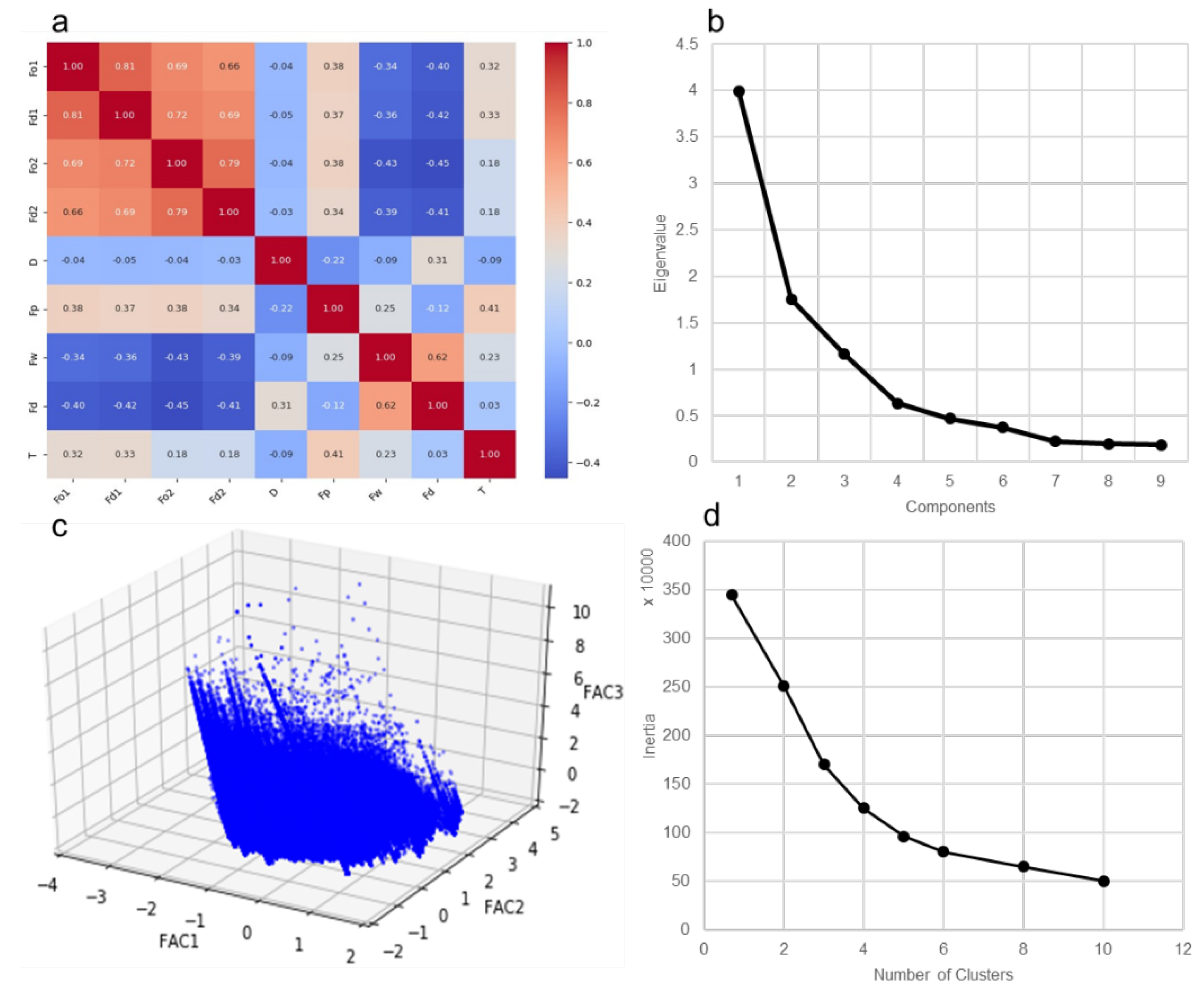
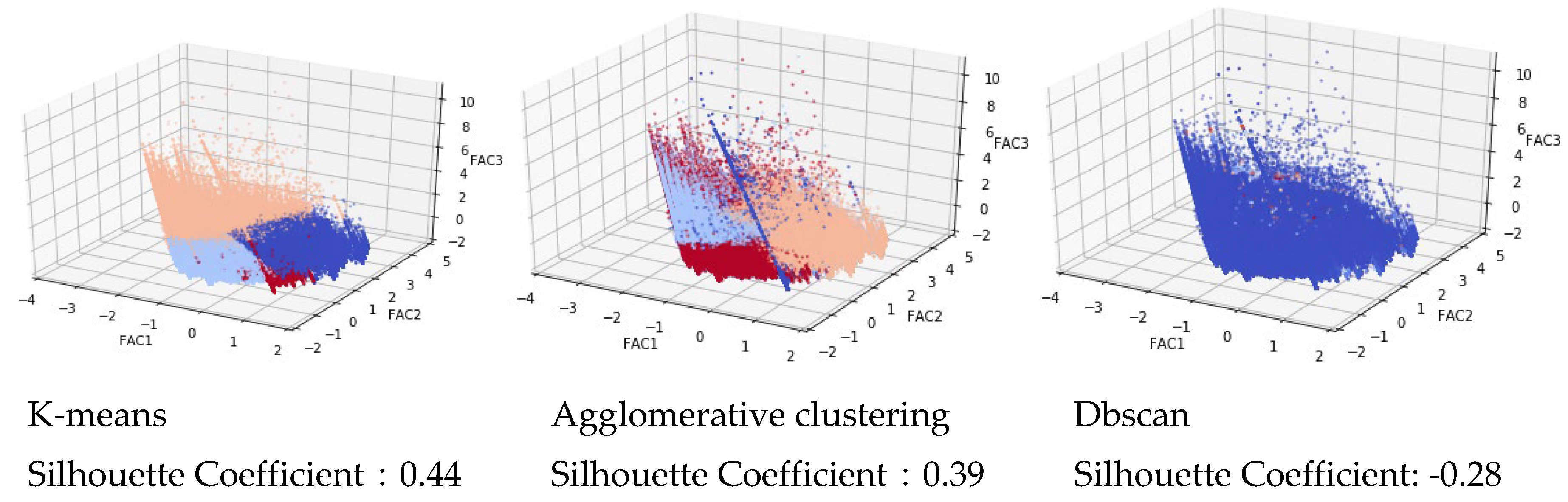
3.1.1. Results of Clustering: Dimensionality Reduction and Clustering Outcomes
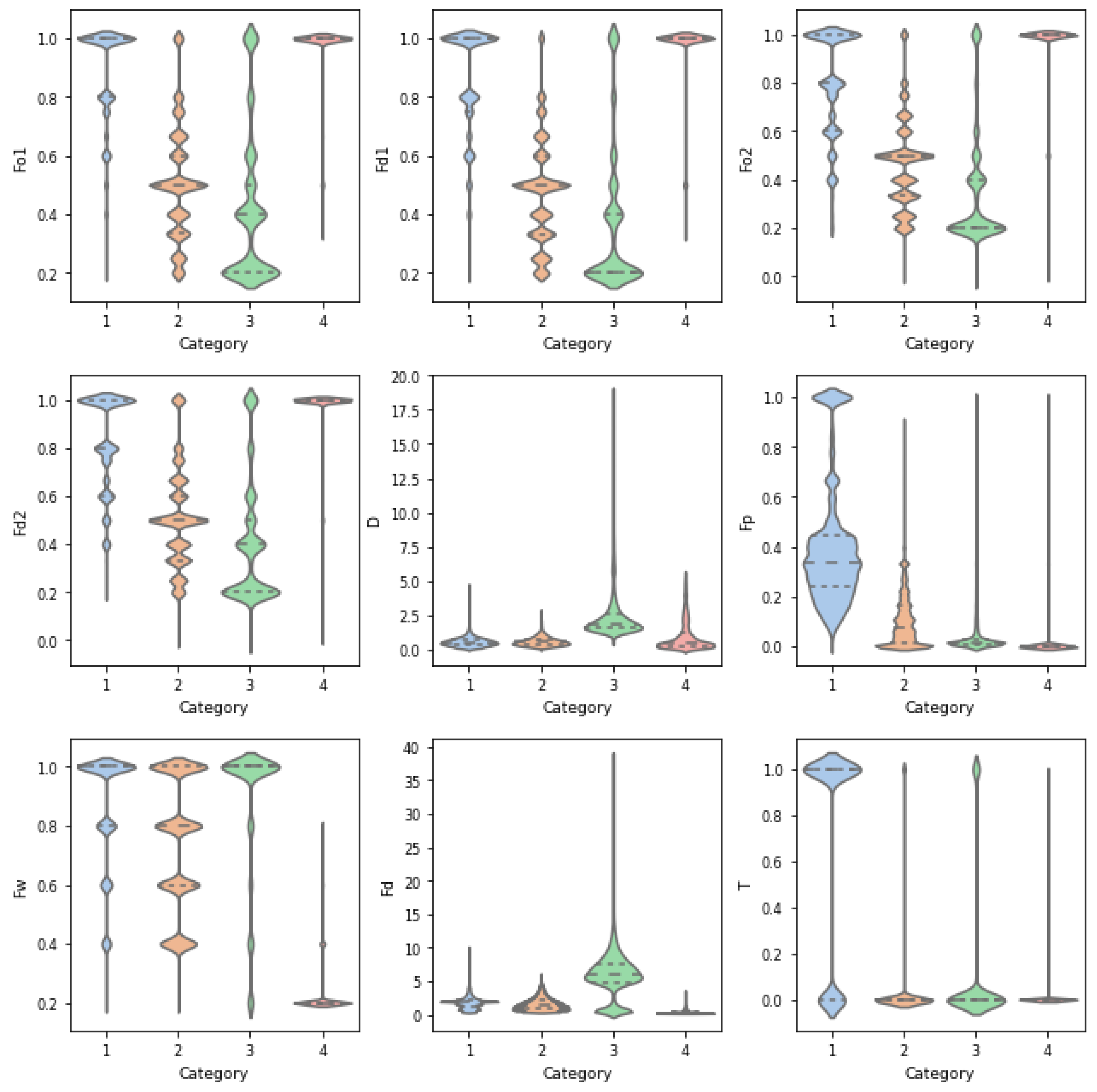
As shown in 0a, there are strong correlations among the features, particularly among the stability coefficients F O 1 F O 1 F D 1 and F D 2 . Consequently, dimensionality reduction was necessary for the feature variables. Prior to dimensionality reduction, the experimental results yielded a KMO value of 0.78 (greater than 0.5) and a Bartlett's test of sphericity p-value of 0.000 (less than 0.05), indicating that the dataset was suitable for dimensionality reduction. As illustrated in 0b, three variables had eigenvalues greater than 1, and the cumulative variance explained by these three principal components reached 77%, effectively capturing the variability in all features. Therefore, three latent variables were extracted from the nine original feature variables after dimensionality reduction. The three-dimensional latent variables obtained through dimensionality reduction are presented in 0c. Finally, the optimal number of travel behavior patterns was determined to be 4 based on the elbow method, as shown in 0d.
Figure 3. Dimensionality reduction and cluster number determination.
Preprints 141852 g003
Figure 4. Clustering results.
Preprints 141852 g004
Based on the method described in Section 2.2.2, we obtained clustering results using three different clustering methods, as shown in 0. The silhouette coefficients for the three clustering methods are 0.44, 0.39, and -0.28, respectively. The K-means clustering algorithm performed the best, followed by the Agglomerative clustering algorithm. The Dbscan algorithm is not suitable for pattern partitioning in this method, possibly due to the uneven distribution of feature indicator data.
After categorizing the travel behavior of 1,144,105 vehicles into four patterns, the distribution and probability density of spatial-temporal feature data for each pattern are presented using violin plots in 0. Additionally, the average features are summarized in 0. 0 illustrates that stability indicators F O 1 , F O 1 , F D 1 , and F D 2 exhibit similar distributions, with multiple peaks observed for patterns 1, 2, and 3, while pattern 4 follows a logarithmic normal distribution. 0 reveals minor differences in the averages of F O 1 , F O 1 , F D 1 , and F D 2 , with patterns 1 and 4 exhibiting high stability at the beginning and end points, pattern 2 at a medium level, and pattern 3 at the lowest level. Notably, pattern 3 displays a logarithmic normal distribution, with the highest average trip distance D , followed by pattern 4, pattern 2, and pattern 1. The similarity distribution of travel paths F p differs across patterns, with pattern 1 exhibiting a peak distribution pattern and patterns 2, 3, and 4 displaying unimodal distributions. Pattern 1 has the highest path similarity, with consistent daily travel paths, while pattern 2 shows lower path similarity, and patterns 3 and 4 have nearly non-repeating travel paths. Regarding weekday travel stability coefficients F w , patterns 1 to 3 show concentrated distributions around 1, indicating almost daily travel, while pattern 2 travels approximately 2-5 days a week, and pattern 4 primarily travels only one day. Furthermore, pattern 3 has the highest average daily travel frequency F d , followed by patterns 1 and 2, which remain stable at around 2 times, while pattern 4 exhibits a daily average travel frequency of approximately 1 to 2 times, representing the lowest travel frequency. In terms of travel time stability, pattern 1 is significantly more stable than the other categories, while pattern 3 displays lower time stability, and patterns 2 and 4 are relatively unconstrained by time.
Table 3. Mean Characteristics.
Travel partterns Fo1 Fd1 Fo2 Fd2 D Fp Fw Fd T
1 0.88 0.86 0.79 0.81 0.28 0.4 0.86 2.09 0.68
2 0.51 0.47 0.46 0.51 0.30 0.1 0.74 2.18 0.04
3 0.42 0.37 0.36 0.41 1.16 0.04 0.89 6.66 0.1
4 0.98 0.97 0.98 0.98 0.49 0.02 0.22 1.59 0
Figure 5. Violin plot of spatiotemporal feature indices.
Preprints 141852 g005
In summary, Pattern 1 shows relatively stable starting and ending points for trips, with consistent weekday travel and a high frequency of daily trips. These trips typically follow fixed routes, with strong time constraints on the first trip of the day, and tend to be short-distance travels. These characteristics align with commuting patterns.
Pattern 2 exhibits moderate stability in starting and ending points, with weekday travel consistency and daily trip frequency similar to Pattern 1. However, the trips are shorter, with less route repetition and no clear time constraints on departure. These trips lack a defined purpose, fitting the irregular travel pattern category.
Pattern 3 shows low stability in starting and ending points but high weekday travel consistency, along with the highest average daily trip frequency and distance. There are few constraints on routes or timing, which is consistent with commercial vehicle usage patterns.
Pattern 4 displays low travel stability, with only one trip recorded during the statistical period. This results in a high level of stability in starting and ending points, suggesting a transit-related pattern.
Therefore, vehicles in Patterns 1 through 4 can be classified as Commuting Vehicles (CVs), Irregular Vehicles (IVs), Commercially Used Vehicles (CUVs), and Transit-Once Vehicles (TVs), respectively.

3.1.2. Recognition Results of Classification Model

Based on the pattern division results, we constructed a classification model suitable for large-scale scenarios following the method outlined in Section 2.2.3. Utilizing nine feature variables, the trained LightGBM classification model achieves an F1-score of 0.99, demonstrating high precision and efficiency in recognition. However, calculating the nine feature variables for a massive number of individuals in large-scale scenarios poses a challenge, exacerbated by the intercorrelations among these variables. Therefore, to address this issue, we ranked the feature importance, as depicted in 0, and tested the impact of different feature quantities on the classification recognition performance, as shown in 0.
Figure 6. Ranking of feature importance.
Preprints 141852 g006
Figure 7. Performance of LightGBM algorithm trained with different numbers of features.
Preprints 141852 g007
From the experimental results, it is evident that relying solely on three feature variables, D F p   a n d   F d , achieves an F1-score of 0.87, indicating satisfactory performance of the classification model. Moreover, the importance of the four feature variables, F O 1 , F O 1 , F D 1 a n d   F D 2 , is similar, and utilizing only one of them yields the same result. Therefore, in large-scale scenarios, efficient recognition of vehicle travel behavior patterns can be achieved by calculating only the three feature variables, D F p   a n d   F d , and subsequently employing the trained classification model for classification.

3.2. Congestion Risk Associated with Different Travel Behavior Patterns

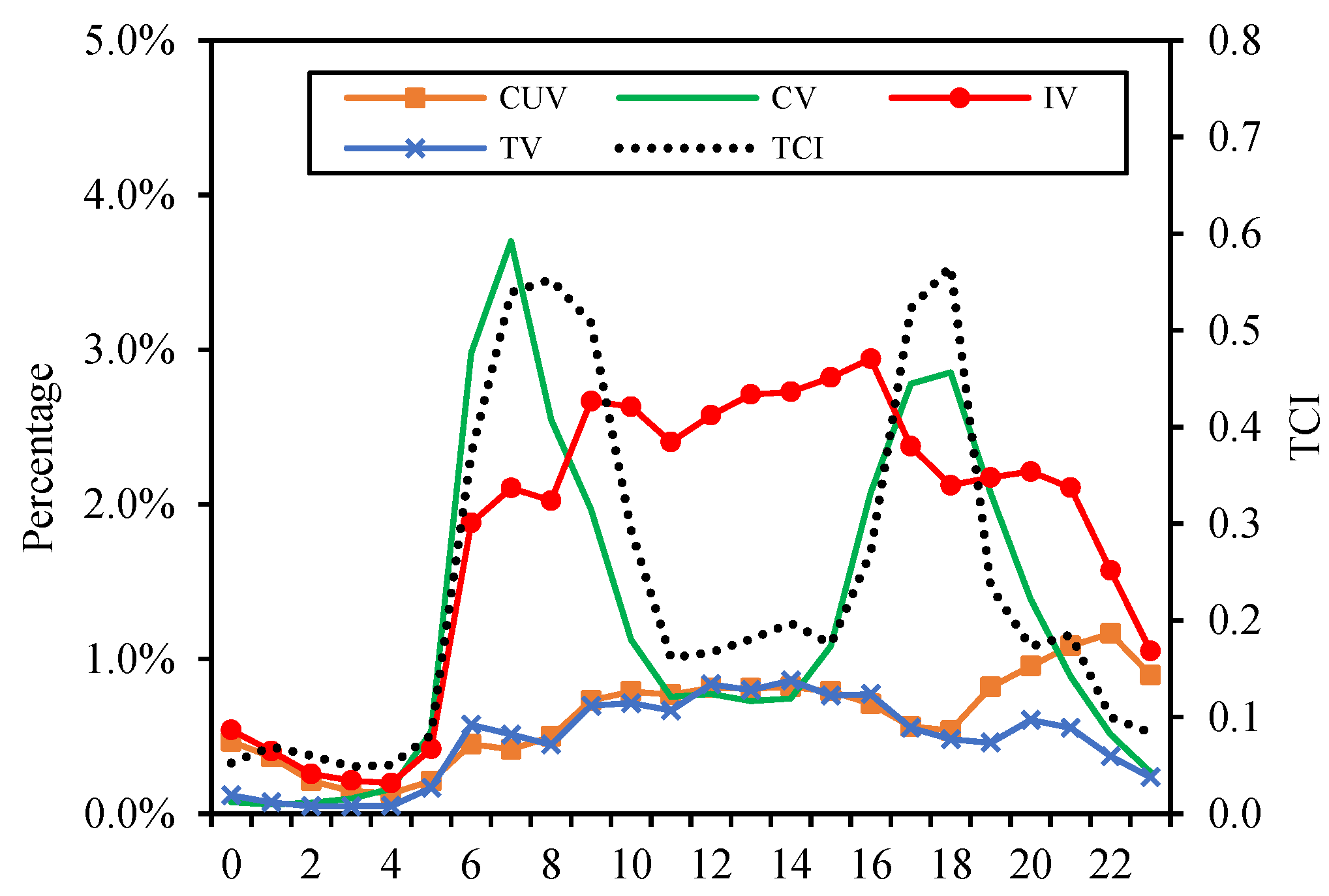
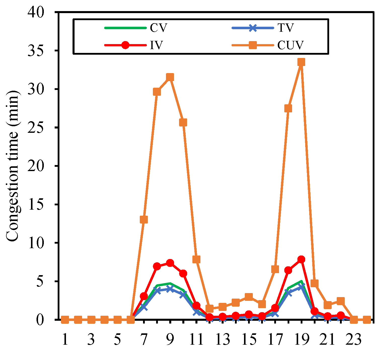
3.2.1. Time Distribution of Congestion for Each Pattern

0 illustrates the time distribution of travel for each pattern. Additionally, we employ an improved Traffic Congestion Index (TCI) to represent the overall traffic condition, as shown in Equation (19), where TCI ranges from [0,1], with higher values indicating greater congestion.
T C I = 1 i = 1 N L i V f r e e _ i W i i = 1 N L i V i W i
where L i is the length of the road segment, W i is the segment weight, V f r e e _ i is the free-flow speed of the segment, and V i is the real-time speed of the segment.
From 0, it can be observed that the CVs pattern peaks during morning and evening rush hours (6:00–10:00 AM and 4:00–8:00 PM), with a higher concentration in the morning compared to the evening. In contrast, the travel patterns of CUVs and TVs on expressways show the opposite trend to CVs, being lower during peak hours and higher during off-peak hours, with CUVs exhibiting increased activity during the evening (7:00–11:00 PM). IVs activity is primarily concentrated between 9:00 AM and 4:00 PM. The trend in the road congestion index aligns with the changes in CVs travel volume, suggesting that the surge in CVs traffic directly contributes to road congestion. When CVs travel volume peaks, road congestion also reaches its highest point. Does this imply that the congestion risk for CVs is the highest?
Figure 8. Time distribution of travel patterns.
Preprints 141852 g008
Additionally, 0 and 0 respectively present the distribution of congestion duration, daily average congestion duration, and the influence of factors such as travel frequency, travel distance, and time preferences on different travel behavior patterns, leading to varying congestion risks. The highest congestion risk is not concentrated in CVs patterns during peak hours, but rather in CUVs patterns that seek to avoid peak-hour travel. Despite accounting for only 15.17% of the total, CUVs patterns can experience congestion for up to three hours a day, with nearly half of this time spent in congested conditions during peak hours. Hence, CUVs drivers intentionally avoid peak hours, preferring to engage in activities such as shift changes and meals during these times, rather than being stuck in traffic. This also explains why the volume of CUVs travel during peak hours in 0 is lower than during off-peak hours. Similarly, TVs patterns also avoid peak-hour travel, while IVs patterns, although not extensively avoiding peak-hour travel, exhibit a slower growth in travel volume during the morning peak period. The second-highest congestion risk is observed in the most prevalent IVs patterns, followed by CVs patterns, with TVs patterns having the lowest congestion risk. Although congestion often occurs during peak hours, the congestion risk for CVs patterns, which are concentrated during peak hours, is comparatively low. Different patterns experience varying levels of congestion risk.
Figure 9. Time Distribution of Congestion Risk for Each Pattern.
Preprints 141852 g009
Figure 10. Proportion of Each Pattern and Daily Average Congestion Duration.
Preprints 141852 g010

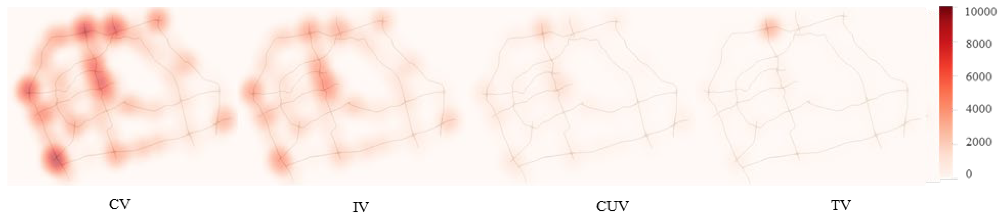
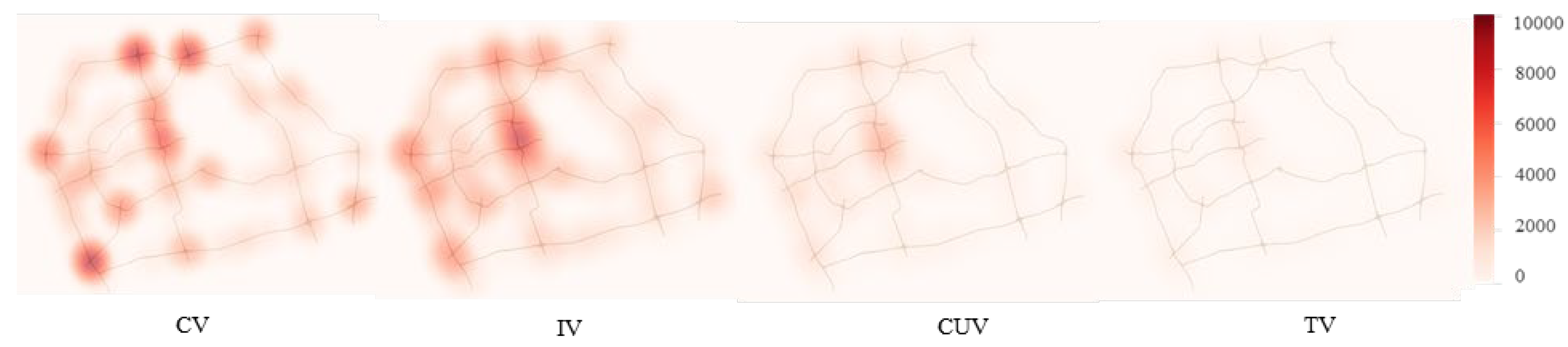
3.2.2. Spatial Distribution of Congestion for Each Pattern

0 and 0 show the kernel density estimates of travel routes for different travel patterns. These figures clearly indicate that congestion occurs at varying locations for each pattern, with congestion points shifting across different time periods. CVs patterns experience congestion primarily on the outer ring and in the city center, suggesting that commuters may live on the outer ring and work in the city center. During the morning peak, CVs patterns show a higher concentration on expressways compared to the evening peak. This can be attributed to two factors: commuters tend to have relatively consistent working hours but varying off-duty hours, and they prefer expressways in the morning to minimize travel time, while they enjoy more flexibility in route choice after work. For TVs patterns, the concentration during the morning peak is also higher than in the evening, with their activities mainly concentrated on the outer ring and passing through the area. In contrast, IVs and CUVs patterns exhibit higher activity levels during the evening peak, as people tend to engage more in dining, entertainment, and leisure activities, which increases the activity of these patterns. Moreover, leisure and entertainment facilities are predominantly located in the city center, leading to higher concentrations of IVs and CUVs patterns in this area.
Furthermore, the congestion points of IVs and CVs patterns overlap significantly, suggesting similarities or a high degree of commonality in their travel routes. CUVs patterns only overlap with CVs patterns in the city center, while TVs patterns overlap with CVs patterns on the outer ring.
Figure 11. Spatial Distribution of Traffic Congestion during Morning Peak Hours.
Preprints 141852 g011
Figure 12. Spatial Distribution of Traffic Congestion during Evening Peak Hours.
Preprints 141852 g012

3.3. Excessive Emissions from Various Patterns

To investigate the additional emissions generated by various patterns during congestion, we explored the excessive emissions of CO. CO emissions associated with traffic are mainly released during vehicle acceleration and deceleration over short periods, which are more relevant in the context of traffic congestion because vehicles involved in congested traffic must accelerate and decelerate frequently [36].
Figure 13. Excessive Emissions from Various Patterns.
Preprints 141852 g013
0 illustrates the distribution of excessive emissions for each pattern. Excessive CO emissions exhibit a trend consistent with the overall traffic flow, showing a bimodal distribution. During the morning peak hours, CO emissions from congestion account for 41% of the total emissions, while during the evening peak, they account for 43%. An interesting phenomenon is that CUVs, accounting for only 15.17% of the total, and IVs, accounting for 43.15%, produce nearly the same amount of excessive CO emissions during peak hours. Although CVs patterns rank third in terms of congestion duration, they have the largest excessive CO emissions. This indicates that commuters do not perceive congestion as significantly as other travelers, but their gas pollution is the largest.

4. Discussion

4.1. Discussion on the Spatiotemporal Characteristics and Congestion Risks of Various Patterns

In this study, we investigate travel behavior patterns and their associated congestion risks using large-scale License Plate Recognition (LPR) data. We classify vehicles into four categories based on travel characteristics such as departure time, route, distance, and frequency: Commercially Used Vehicles (CUVs) (15.17%), Commuting Vehicles (CVs) (30.25%), Irregular Vehicles (IVs) (43.15%), and Transit-once Vehicles (TVs) (11.43%).
CVs exhibit strong spatiotemporal stability, with an average of two trips per day on workdays, stable first departure times (fluctuating by less than 30 minutes on average, predominantly during morning peak hours), consistent commuting routes, and typically short to medium travel distances. CUVs, in contrast, have a higher daily frequency of travel and longer distances. IVs have travel frequencies and distances similar to CVs, but lack spatiotemporal stability, resembling non-commuting family vehicles. TVs, which pass through only once, lack any spatiotemporal stability features.
Although congestion risks for all patterns follow a bimodal distribution, the duration of congestion varies across patterns. The temporal distribution of travel frequencies and routes differs for each pattern, leading to varying congestion durations. CUVs, with high travel frequencies and concentration in downtown areas, experience the longest congestion durations, while CVs, which are concentrated during peak congestion periods, encounter shorter durations.
Furthermore, despite comprising only 15.17% of the total vehicle count, CUVs contribute excess CO emissions from congestion equivalent to those of IVs, which make up 43.15% of the total. This suggests that accurate estimation of congestion risks and emissions requires consideration of all travel patterns. Focusing exclusively on CVs or CUVs may significantly underestimate congestion risks.

4.2. Discussion on Strategies to Reduce Congestion Risks

By identifying travel patterns and estimating congestion risks, relevant authorities can develop targeted strategies to manage demand and effectively reduce congestion. This paper evaluates the contribution of each travel pattern to congestion, with the following proportions: CUVs (15.17%), CVs (30.25%), IVs (43.15%), and TVs (11.43%). The data indicate that approximately 12.6% of road congestion during peak hours results from overload, meaning that 87.4% of travel demand can be accommodated, while the remaining 12.6% contributes to congestion. Although different vehicles may follow distinct travel patterns, they all have equal rights to access the road. Thus, completely restricting certain vehicle types, such as CUVs or TVs, from entering expressways during peak hours may raise concerns.
Furthermore, different travel patterns have varying route scopes. For instance, banning CUVs from expressways may not alleviate congestion on outer loops. Each pattern also presents different congestion risks and emission levels. While current research often focuses on CVs, commuting vehicles typically do not face high congestion risks. In contrast, CUVs, which receive less attention, encounter significant congestion risks and generate higher emissions. Therefore, congestion management strategies should account for the diverse travel characteristics of each pattern and integrate them accordingly. Focusing solely on a specific vehicle type is insufficient.
The surge of CVs during peak hours is one of the direct causes of congestion. If at least 12.6% of vehicles can be dispersed during peak hours, reducing the concentration of vehicles in the same spatiotemporal space, congestion relief can be achieved. Moreover, with economic development, the number of motor vehicles will continue to rise, accompanied by an increase in "conservative" vehicles—those that rely on private cars for all trips [37], with low willingness to use shared or public transportation [38,39,40,41]. A transition from private car travel to public transportation will require a long period. Therefore, inducing different travel patterns in spatiotemporal dimensions is an efficient and equitable strategy [42,43]. By considering the spatiotemporal characteristics of each pattern, guiding travel routes at different times can align with travelers' route preferences and help alleviate road congestion [44]. For example, guiding the route preferences of CVs can directly assist traffic management authorities in designing more feasible and effective route planning schemes, which can then inform the planning of travel routes for other vehicles. Targeted control of the most congested travelers can maximize congestion and emission reduction [45,48].
This study does have some limitations. Firstly, to analyze congestion risks and emissions associated with various travel patterns, only weekday data were considered, and weekend travel patterns were not examined. Secondly, while we proposed a comprehensive framework for pattern classification and recognition, this study focused only on expressway networks and did not include the entire urban road network. As a result, some vehicle trajectories may not fully represent travel records. In the future, we plan to collect data from a broader spatiotemporal scope to further enhance the study of travel patterns. We also intend to explore route induction under different travel pattern classifications.

5. Conclusions

This study investigates congestion risks and excess emissions associated with various travel behavior patterns using comprehensive LPR data from urban expressways. First, we propose a pattern recognition method based on the spatiotemporal information embedded in LPR data, designed for large-scale applications. We then analyze the spatiotemporal characteristics of different travel patterns, examining their corresponding traffic congestion risks and excess emissions.
The findings reveal a bimodal distribution of congestion risks across various patterns. The magnitude of congestion risk is closely linked to the travel characteristics of each pattern, with congestion hotspots concentrated in downtown areas and outer loops. Interestingly, the highest congestion risk does not occur with commuting vehicles, despite their concentration during peak hours. Focusing solely on commuting vehicles may severely underestimate both congestion risks and emissions, potentially rendering congestion mitigation strategies ineffective.
This research enhances our understanding of the relationship between individual travel behavior and traffic congestion, providing valuable insights for personal travel time planning and health management. Furthermore, the methodology and conclusions presented in this paper can inform the development of personalized, proactive traffic demand management strategies.

Funding

the National Key Research and Development Program of China 2023YFB4301900, Shenzhen Science and Technology Program JSGG20220831094604008, Key-Area Research and Development Program of Guangdong Province 2022B0101070002.

Acknowledgments

The authors confirm the following contributions to this paper: Research concept and design: Zhaocheng He, Yuting Wang; Data collection: Zhaocheng He, Yuting Wang; Analysis and interpretation of results: Zhaocheng He, Yuting Wang, Wangyong Xing; First draft preparation: Yuting Wang, Chengchuang Lin. All authors reviewed the results and approved the final version of the manuscript.

Disclosure statement

No potential conflict of interest was reported by the authors.

Data availability statement

The participants of this study did not give written consent for their data to be shared publicly, so due to the sensitive nature of the research supporting data is not available.

References

  1. Sandow, E.; Westerlund, O.; Lindgren, U. Is Your Commute Killing You? On the Mortality Risks of Long-Distance Commuting. Environ. Plan. Econ. Space 2014, 46, 1496–1516. [Google Scholar] [CrossRef]
  2. Currie, J.; Walker, R. Traffic Congestion and Infant Health: Evidence from E-ZPass. Am. Econ. J. Appl. Econ. 2011, 3, 65–90. [Google Scholar] [CrossRef]
  3. Bigazzi, A. Y.; Figliozzi, M. A.; Clifton, K. J. Traffic Congestion and Air Pollution Exposure for Motorists: Comparing Exposure Duration and Intensity. Int. J. Sustain. Transp. 2015, 9, 443–456. [Google Scholar] [CrossRef]
  4. Wu, W.; Wang, M. (Xin); Zhang, F. Commuting Behavior and Congestion Satisfaction: Evidence from Beijing, China. Transp. Res. Part Transp. Environ. 2019, 67, 553–564. [Google Scholar] [CrossRef]
  5. Deng, J.; Cui, Y.; Chen, X.; Bachmann, C.; Yuan, Q. Who Are on the Road? A Study on Vehicle Usage Characteristics Based on One-Week Vehicle Trajectory Data. Int. J. Digit. Earth 2023, 16, 1962–1984. [Google Scholar] [CrossRef]
  6. KhorramDehnavi, S.; MorovatiSharifabadi, A.; AghidiKheyrabadi, S.; HosseiniBamakan, S. M. Evaluating Private Car Users’ Preference to Congestion Pricing: A Study on Trip Cancellation Behavior. Case Stud. Transp. Policy 2024, 18, 101300. [Google Scholar] [CrossRef]
  7. Dong, Y.; Wang, S.; Li, L.; Zhang, Z. An Empirical Study on Travel Patterns of Internet Based Ride-Sharing. Transp. Res. Part C Emerg. Technol. 2018, 86, 1–22. [Google Scholar] [CrossRef]
  8. Chen, X. (Michael); Zahiri, M.; Zhang, S. Understanding Ridesplitting Behavior of On-Demand Ride Services: An Ensemble Learning Approach. Transp. Res. Part C Emerg. Technol. 2017, 76, 51–70. [Google Scholar] [CrossRef]
  9. Wang, F.; Wang, J.; Cao, J.; Chen, C.; Ban, X. (Jeff). Extracting Trips from Multi-Sourced Data for Mobility Pattern Analysis: An App-Based Data Example. Transp. Res. Part C Emerg. Technol. 2019, 105, 183–202. [Google Scholar] [CrossRef]
  10. Badiola, N.; Raveau, S.; Galilea, P. Modelling Preferences towards Activities and Their Effect on Departure Time Choices. Transp. Res. Part Policy Pract. 2019, 129, 39–51. [Google Scholar] [CrossRef]
  11. Rahman, M.; Akther, S. Intercity Commuting in Metropolitan Regions: A Mode Choice Analysis of Commuters Traveling to Dhaka from Nearby Cities. J. Urban Plan. Dev. 2022, 148. [Google Scholar] [CrossRef]
  12. Rafiq, R.; McNally, M. G. A Structural Analysis of the Work Tour Behavior of Transit Commuters. Transp. Res. Part Policy Pract. 2022, 160, 61–79. [Google Scholar] [CrossRef]
  13. Jiang, S.; Yang, Y.; Gupta, S.; Veneziano, D.; Athavale, S.; González, M. C. The TimeGeo Modeling Framework for Urban Motility without Travel Surveys. Proc. Natl. Acad. Sci. U. S. A. 2016, 113, E5370–E5378. [Google Scholar] [CrossRef]
  14. Chen, H.; Cai, M.; Xiong, C. Research on Human Travel Correlation for Urban Transport Planning Based on Multisource Data. Sensors 2021, 21. [Google Scholar] [CrossRef]
  15. Guo, Y.; Yang, F.; Yan, H.; Xie, S.; Liu, H.; Dai, Z. Activity-Based Model Based on Multi-Day Cellular Data: Considering the Lack of Personal Attributes and Activity Type. IET Intell. Transp. Syst. n/a. [CrossRef]
  16. Zheng, Y.; Capra, L.; Wolfson, O.; Yang, H. Urban Computing: Concepts, Methodologies, and Applications. ACM Trans. Intell. Syst. Technol. 2014, 5. [Google Scholar] [CrossRef]
  17. Li, Z.; Xiong, G.; Wei, Z.; Zhang, Y.; Zheng, M.; Liu, X.; Tarkoma, S.; Huang, M.; Lv, Y.; Wu, C. Trip Purposes Mining From Mobile Signaling Data. IEEE Trans. Intell. Transp. Syst. 2022, 23, 13190–13202. [Google Scholar] [CrossRef]
  18. Chen, Y.; Wang, Z.; Sun, H.; Wang, J. Exploring Activity Patterns and Trip Purposes of Public Transport Passengers from Smart Card Data. J. Transp. Eng. Part Syst. 2023, 149. [Google Scholar] [CrossRef]
  19. Liu, Z.; Li, R.; Wang, X.; Shang, P. Effects of Vehicle Restriction Policies: Analysis Using License Plate Recognition Data in Langfang, China. Transp. Res. Part Policy Pract. 2018, 118, 89–103. [Google Scholar] [CrossRef]
  20. Chang, Y.; Duan, Z.; Yang, D. Using ALPR Data to Understand the Vehicle Use Behaviour under TDM Measures. IET Intell. Transp. Syst. 2018, 12, 1264–1270. [Google Scholar] [CrossRef]
  21. Goulet-Langlois, G.; Koutsopoulos, H. N.; Zhao, Z.; Zhao, J. Measuring Regularity of Individual Travel Patterns. IEEE Trans. Intell. Transp. Syst. 2018, 19, 1583–1592. [Google Scholar] [CrossRef]
  22. Sun, L.; Chen, X.; He, Z.; Miranda-Moreno, L. F. Routine Pattern Discovery and Anomaly Detection in Individual Travel Behavior. Netw. Spat. Econ. 2023, 23, 407–428. [Google Scholar] [CrossRef]
  23. Yao, W.; Zhang, M.; Jin, S.; Ma, D. Understanding Vehicles Commuting Pattern Based on License Plate Recognition Data. Transp. Res. Part C Emerg. Technol. 2021, 128, 103142. [Google Scholar] [CrossRef]
  24. Wan, L.; Tang, J.; Wang, L.; Schooling, J. Understanding Non-Commuting Travel Demand of Car Commuters – Insights from ANPR Trip Chain Data in Cambridge. Transp. Policy 2021, 106, 76–87. [Google Scholar] [CrossRef]
  25. Berrill, P.; Nachtigall, F.; Javaid, A.; Milojevic-Dupont, N.; Wagner, F.; Creutzig, F. Comparing Urban Form Influences on Travel Distance, Car Ownership, and Mode Choice. Transp. Res. Part Transp. Environ. 2024, 128, 104087. [Google Scholar] [CrossRef]
  26. Lian, T.; Loo, B. P. Y. Cost of Travel Delays Caused by Traffic Crashes. Commun. Transp. Res. 2024, 4, 100124. [Google Scholar] [CrossRef]
  27. Higgins, C. D.; Sweet, M. N.; Kanaroglou, P. S. All Minutes Are Not Equal: Travel Time and the Effects of Congestion on Commute Satisfaction in Canadian Cities. Transportation 2018, 45, 1249–1268. [Google Scholar] [CrossRef]
  28. Beland, L.-P.; Brent, D. A. Traffic and Crime. J. Public Econ. 2018, 160, 96–116. [Google Scholar] [CrossRef]
  29. Yildirimoglu, M.; Ramezani, M.; Amirgholy, M. Staggered Work Schedules for Congestion Mitigation: A Morning Commute Problem. Transp. Res. Part C Emerg. Technol. 2021, 132, 103391. [Google Scholar] [CrossRef]
  30. Ravalet, E.; Rérat, P. Teleworking: Decreasing Mobility or Increasing Tolerance of Commuting Distances? Built Environ. 2019, 45, 582–602. [Google Scholar] [CrossRef]
  31. Chen, H.; Yang, C.; Xu, X. Clustering Vehicle Temporal and Spatial Travel Behavior Using License Plate Recognition Data. J. Adv. Transp. 2017, 2017, e1738085. [Google Scholar] [CrossRef]
  32. Alessandretti, L.; Lehmann, S. Trip Frequency Is Key Ingredient in New Law of Human Travel. Nature 2021, 593, 515–516. [Google Scholar] [CrossRef] [PubMed]
  33. Warne, R. T.; Larsen, R. Evaluating a Proposed Modification of the Guttman Rule for Determining the Number of Factors in an Exploratory Factor Analysis. Psychol. Test Assess. Model. 2014, 56, 104–123. [Google Scholar]
  34. Kan, Z.; Kwan, M.-P.; Liu, D.; Tang, L.; Chen, Y.; Fang, M. Assessing Individual Activity-Related Exposures to Traffic Congestion Using GPS Trajectory Data. J. Transp. Geogr. 2022, 98, 103240. [Google Scholar] [CrossRef]
  35. Yang, D.; Zhang, S.; Niu, T.; Wang, Y.; Xu, H.; Zhang, K. M.; Wu, Y. High-Resolution Mapping of Vehicle Emissions of Atmospheric Pollutants Based on Large-Scale, Real-World Traffic Datasets. Atmospheric Chem. Phys. 2019, 19, 8831–8843. [Google Scholar] [CrossRef]
  36. Zhang, K.; Batterman, S.; Dion, F. Vehicle Emissions in Congestion: Comparison of Work Zone, Rush Hour and Free-Flow Conditions. Atmos. Environ. 2011, 45, 1929–1939. [Google Scholar] [CrossRef]
  37. Baro, R.; Rao, K. V. K.; Velaga, N. R. Role of Private Vehicle Commuters’ Travel Wellbeing Perception in Mode Shift Behavior towards an Upcoming Metro in Mumbai Metropolitan Region. Case Stud. Transp. Policy 2024, 16, 101210. [Google Scholar] [CrossRef]
  38. Li, W.; Kamargianni, M. Steering Short-Term Demand for Car-Sharing: A Mode Choice and Policy Impact Analysis by Trip Distance. Transportation 2020, 47, 2233–2265. [Google Scholar] [CrossRef]
  39. van ’t Veer, R.; Annema, J. A.; Araghi, Y.; Homem de Almeida Correia, G.; van Wee, B. Mobility-as-a-Service (MaaS): A Latent Class Cluster Analysis to Identify Dutch Vehicle Owners’ Use Intention. Transp. Res. Part Policy Pract. 2023, 169, 103608. [Google Scholar] [CrossRef]
  40. Wei, B.; Zhang, X.; Liu, W.; Saberi, M.; Waller, S. T. Capacity Allocation and Tolling-Rewarding Schemes for the Morning Commute with Carpooling. Transp. Res. Part C Emerg. Technol. 2022, 142, 103789. [Google Scholar] [CrossRef]
  41. Lavieri, P. S.; Bhat, C. R. Modeling Individuals’ Willingness to Share Trips with Strangers in an Autonomous Vehicle Future. Transp. Res. Part Policy Pract. 2019, 124, 242–261. [Google Scholar] [CrossRef]
  42. Zhang, Y.; Zhao, H.; Jiang, R. Manage Morning Commute for Household Travels with Parking Space Constraints. Transp. Res. Part E Logist. Transp. Rev. 2024, 185, 103504. [Google Scholar] [CrossRef]
  43. Feng, X.; Lin, Q.; Jia, N.; Tian, J. The Actual Impact of Ride-Splitting: An Empirical Study Based on Large-Scale GPS Data. Transp. Policy 2024, 147, 94–112. [Google Scholar] [CrossRef]
  44. (44) Deng, J.; Li, T.; Yang, Z.; Yuan, Q.; Chen, X. Heterogeneity in Route Choice during Peak Hours: Implications on Travel Demand Management. Travel Behav. Soc. 2025, 38, 100922. [Google Scholar] [CrossRef]
  45. Chaudhry, S. K.; Elumalai, S. P. Assessment of Sustainable School Transport Policies on Vehicular Emissions Using the IVE Model. J. Clean. Prod. 2024, 434, 140437. [Google Scholar] [CrossRef]
  46. Abbiasov, T.; Heine, C.; Sabouri, S.; Salazar-Miranda, A.; Santi, P.; Glaeser, E.; Ratti, C. The 15-Minute City Quantified Using Human Mobility Data. Nat. Hum. Behav. 2024, 8, 445–455. [Google Scholar] [CrossRef]
  47. Zong, F.; Zeng, M.; Li, Y.-X. Congestion Pricing for Sustainable Urban Transportation Systems Considering Carbon Emissions and Travel Habits. Sustain. Cities Soc. 2024, 101, 105198. [Google Scholar] [CrossRef]
  48. Geng, Y.; Zhang, X.; Gao, J.; Yan, Y.; Chen, L. Bibliometric Analysis of Sustainable Tourism Using CiteSpace. Technol. Forecast. Soc. Change 2024, 202, 123310. [Google Scholar] [CrossRef]
Disclaimer/Publisher’s Note: The statements, opinions and data contained in all publications are solely those of the individual author(s) and contributor(s) and not of MDPI and/or the editor(s). MDPI and/or the editor(s) disclaim responsibility for any injury to people or property resulting from any ideas, methods, instructions or products referred to in the content.
Copyright: This open access article is published under a Creative Commons CC BY 4.0 license, which permit the free download, distribution, and reuse, provided that the author and preprint are cited in any reuse.
Prerpints.org logo

Preprints.org is a free preprint server supported by MDPI in Basel, Switzerland.

Subscribe

Disclaimer

Terms of Use

Privacy Policy

Privacy Settings

© 2025 MDPI (Basel, Switzerland) unless otherwise stated