
Submitted:
03 December 2024
Posted:
04 December 2024
You are already at the latest version
Abstract
This investigation presents the current status of seismic sedimentology, as applied to high-resolution (<5m) mapping of sedimentary facies and hydrocarbon reservoirs in the subsurface. Seismic sedimentology involves the integrated study of seismic lithology and seismic geomorphology. High-resolution lithology, thickness, and geobody geometry mapping can be achieved by focusing on spatial resolution, data quality, attribute selection, seismic modeling, and application of machine learning techniques. As their geophysical counterparts, the interpreters with geologic background can do as good in seismic sedimentology.
Keywords:
Seismic sedimentology
; seismic resolution
; spatial resolution
; thin-bed
; reservoir
1. Introduction
What is seismic sedimentology? Since Zeng et al. (1998) used the word for the first time, consensus has evolved. In reservoir geophysics (Johnston, 2010), seismic lithology is the use of seismic attributes in predicting lithology types, such as sandstone, shale, carbonates, and evaporates. Posamentier (2001) uses the term seismic geomorphology to describe the seismic pattern of depositional geomorphology in a plane or 3D view. Schlager (2000) proposes seismic sedimentology as a tool of sedimentary research that aims at imaging, interpretation, and modeling of seismic-wave responses of layered sedimentary rocks. Zeng and Hentz (2004) define seismic sedimentology as the seismic investigation of sedimentary rocks and depositional processes by the combined study of seismic lithology and seismic geomorphology, emphasizing the complementary nature of the two.
Seismic stratigraphy, introduced by Vail et al. in 1977, was developed for the low-resolution (50-500 m thick) analysis of basin-scale depositional systems. In response to the growing need for high-resolution thin-bed mapping in sedimentary basins, seismic sedimentology emerged using seismic data. After decades of intensive exploration and development, most of the more accessible hydrocarbon plays in thick reservoir sequences have been discovered. The remaining hydrocarbon potential primarily lies in thin-beds, such as those less than 5 meters thick, particularly in non-marine basins in China and elsewhere (Zhu et al., 2020). Currently, both thin-bedded conventional reservoirs and shale-oil formations are receiving significant attention. The ongoing discussion about improving seismic resolution is timely, as it focuses on enhancing the prediction of these thin-beds.
Seismic resolution is a broad topic that encompasses various aspects essential for understanding and improving it (Zeng 2024). These aspects address designing and acquiring 3D surveys, processing, and interpretation. Given the limited scope of this paper, it is impractical to cover all these areas thoroughly. Instead, I will focus on the third aspect: interpretation. In this discussion, I will clarify what by high-resolution facies mapping means using seismic data, and how seismic sedimentology can achieve better facies resolution. While this discussion may not cover every detail, I hope to present valuable concepts and methods that will benefit our geologic colleagues.
2. Current Understanding of Seismic Resolution
The concept of seismic resolution evolves with time. Various definitions have been established over the past five decades based on different criteria (Zeng 2024). Notably, Kallweit and Wood’s (1982) “peak-to-trough” or Rayleigh’s criteria have become widely accepted. They demonstrated to most interpreters that, for a wedge with a stepwise impedance profile (see Figure 1), the resolution limit is most practically defined by the “peak-to-trough” separation of the composite waveform at λ/4 (where λ is the dominant wavelength, typically between 15 and 150 meters). For a wedge with a box impedance profile, this corresponds to the “turning point,” where the maximum composite amplitude is measured (see Figure 2). The concept of resolution is closely tied to our cognitive understanding of the geologic subject (e.g., a feature, a 2D bed, or a 3D body). New concepts may emerge in the future to accommodate new interpretational demands. In addition, the definition of seismic resolution is derived from an idealized earth model and represents the best theoretical resolution. However, the actual resolution is not always as high as the theoretical resolution, partly due to imperfect interpretation. Our goal is to find more efficient techniques and workflows to improve the actual resolution.
3. Quality of Seismic Data
The quality of seismic data is crucial for accurate stratigraphic and sedimentological interpretation. Over the last several decades, academia and industry have significantly advanced data acquisition and processing. Modern digital seismic data typically feature a wide frequency range of 10 to 100 Hz, utilize a zero-phase wavelet, maintain precise 3D positioning in migrated data, and possess a satisfactory signal-to-noise ratio. We can still perform various analyses even with imperfect data—such as numerous legacy 3D data sets collected in the 1980s and 1990s. Numerous published case studies of seismic geomorphology and seismic sedimentology from the last thirty years rely on these legacy data sets (e.g., Posamentier, 2002; Zeng and Hentz, 2004; Dong et al., 2008).
Geologic interpreters can seek assistance from geophysicists to achieve cost-effective improvements in data quality through reprocessing and specialized processing techniques. For example, significant efforts have been made to enhance data processing for higher seismic resolution. A common approach is to extrapolate or to reshape the bandwidth using poststack data, for instance spectral balancing (e.g., Fehmers and Höcker, 2003), spectral inversion (e.g., Portniaguine and Castagna, 2004), bandwidth extension (Smith et al., 2008), and pseudo deconvolution (Matos and Marfurt, 2011).
This section may be divided by subheadings. It should provide a concise and precise description of the experimental results, their interpretation, as well as the experimental conclusions that can be drawn.
4. Seismic Attributes for Seismic Lithology
For the digital seismic data delivered to interpreters after processing, the main aspects influencing actual resolution include choice of attributes, selection of frequency bandwidth, and the wavelet shape. Certain strategies are more effective for particular geologic and geophysical studies, such as stratigraphy, sedimentology, structure, rock physics, or fluid content. A comprehensive understanding of these issues requires an extensive literature review. This section will concentrate specifically on effective strategies for stratigraphic and sedimentological interpretations.
1. Choice of attributes: Many seismic attributes can relate seismic signals to a reservoir formation’s acoustic impedance, lithology, and porosity profile. To list a few, 90° phase trace, integrated trace, and model-based inversion are all valuable attributes. Based on the author’s experience, 90° phase trace is geologist-friendly and preferred (see discussion in the next section). At the same time, seismic waveform (trace) is still the primary platform for interpretation. Some noteworthy attributes can indicate thin beds at or below seismic resolution (thin-bed indicators). Thin-bed attributes include instantaneous attributes (Taner & Sheriff, 1977), singularity (Liner et al., 2004; Li and Liner, 2005, 2008), and phase residues (Matos et al., 2011), among others.
2. Wavelet shape and compactness: Seismic interpreters often prefer using zero-phase wavelets due to their symmetric waveform, which offers the most compact representation and the highest temporal resolution (Brown, 1991). However, this advantage applies primarily when analyzing a single reflection surface, such as in structural mapping. If the subject is a thin-bed (see Figure 2), the composite waveform becomes antisymmetric, removing the benefits of the symmetric wavelet. Researchers can employ a 90° wavelet to recreate a symmetric waveform to address this issue while preserving compactness and optimal resolution (e.g., Siding, 1982) (see Figure 3).
When comparing a series of stratal slices created from 90° data to those derived from a zero-phase volume within the same strata, interpreters will notice that the 90° slice series displays fewer channel fingerprints. This difference is because there is less vertical mixing of the stacked events, leading to reduced interference. This method is particularly effective for interpreting interbedded thin-bed sequences.
3. Strategies to use frequency information: Over the last three decades, seismic frequency information analysis and application have significantly progressed. Partyka et al. (1999) invented the spectral decomposition method, utilizing the short window discrete Fourier transform (SWDFT) to calculate the spectral energy for time-frequency cubes. In contrast, Grossmann and Morlet (1984) developed the continuous wavelet transform (CWT), which cross-correlates a set of wavelets against a traveltime series to create localized frequency images of seismic traces in time. This method was refined by matching pursuit decomposition (MPD) to achieve higher vertical resolution in the frequency domain (Mallat and Zhang, 1992; Castagna and Sun, 2006).
Moreover, eliminating the interference of low-frequency components from high-frequency subvolumes can significantly enhance seismic resolution for thin beds. A more effective approach is RGB color blending of high-, moderate-, and low-frequency spectral components or seismic travel time traces; this is also called frequency fusion (Zeng, 2017). Notably, when using 90° data, frequency fusion allows for integrating both thick and thin-beds in the vertical view. As a result, the typically constant width of seismic events in conventional stacked and migrated color display (Figure 4a) aligns more accurately with the true thickness of lithofacies bodies (in this case, sand bodies a through g, Figure 4b) without substantial interference.
In the horizontal view, broken images of channels in the conventional display (#1 - #7, Figure 4c) appear more continuous, revealing more realistic, thickness-adjusted channel geometry (Figure 4d). Additionally, frequency fusion proves advantageous for the stratigraphic and sedimentological reconstruction of a formation in the vertical view. It creates a display illustrating lithofacies and stratigraphic cyclicity, resembling outcrop photos (Figure 5a). In contrast, MPD-processed frequency decomposition in the frequency domain does not achieve the same effect (Figure 5b).
5. Horizontal Resolution and Seismic Geomorphology
If processed correctly, the horizontal resolution of a 3D seismic cube should be roughly equal to its vertical resolution (Lindsey, 1989). However, the effectiveness of either resolution in interpretation depends on the stacking pattern of lithofacies in the geological strata. The ratio of the horizontal to vertical dimensions of a lithofacies unit determines its spatial resolution status.
From outcrop observations, most of the thin sedimentary units are large in horizontal dimensions (tens to thousands of meters) and small in vertical dimensions (several meters to tens of meters). Such thin beds can generally be one-way resolved in the horizontal dimension, but can only be detected in the vertical dimension. Thin-beds are volumetrically critical in both marine and lacustrine formations. Fortunately, many of these beds can be effectively interpreted using seismic geomorphology on stratal slices. The seismic interpretation of thin-beds is limited to what can be detected. In a case study, we found that, with wireline log verification, distributary channel sands as thin as one meter (λ/80) can be spatially resolved (Figure 6)—much thinner than λ/25 speculated by Sheriff (1991) decades ago.
Seismic geomorphology can be performed using time, horizon, and stratal slices (Posamentier et al., 1996; Zeng et al., 1998), as long as they are made following geologic-time equivalent, depositional surface. Ideally, stratal slices are the preferred option, as they are created by proportional slicing between two reference geologic events (e.g., maximum flooding surfaces) without significant internal depositional hiatuses (e.g., angular unconformities).
6. Seismic modeling is a bridge
Seismic modeling is useful for finding a true link between seismic lithology, geomorphology, and facies and for recognizing and avoiding pitfalls. Unlike complex structural and rock-physical modeling (e.g., many models discussed in the SEAL project of the Society of Exploration Geophysicists), geologic and seismic models do not have to be over-sophisticated for many sedimentary interpretations. Being able to be created and interpreted by geologists, simple acoustic, convolutional models are adequate unless approved otherwise. When elastic and wave-equation-guided modeling is needed, geophysicists can provide critical help.
Although modeling is case-sensitive in general and should be performed according to specific geologic and geophysical conditions, some important lessons can be easily summarized from simple, convolutional models:
1. For a typical, interfingered sand-shale profile, a 90° phase trace is a reasonable estimation for acoustic impedance and, therefore, for lithofacies (Figure 3);
2. Maximum amplitude at λ/4 defines seismic resolvable limit and, at the same time, illustrates amplitude tuning phenomenon that is a pitfall to porosity mapping (Figure 2 and Figure 3);
3. Seismic onlap or downlap patterns do not necessarily indicate the true pinch-out points of lithofacies (e.g., Biddle et al., 1992);
4. Seismic reflections do not necessarily follow geologic-time surfaces (Tipper, 1993); stratal slices are better choices for sedimentary facies imaging (Zeng et al., 1998);
5. For a thin and shingled progradational sequence common in shallow-water deltaic systems or prograding carbonate platforms (Figure 7a), seismic clinoforms are difficult to recognize in the vertical section (Figure 7b) but more visible in a horizontal view (Figure 7c), showing the power of horizontal seismic resolution.
7. Machine Learning Comes to Help!
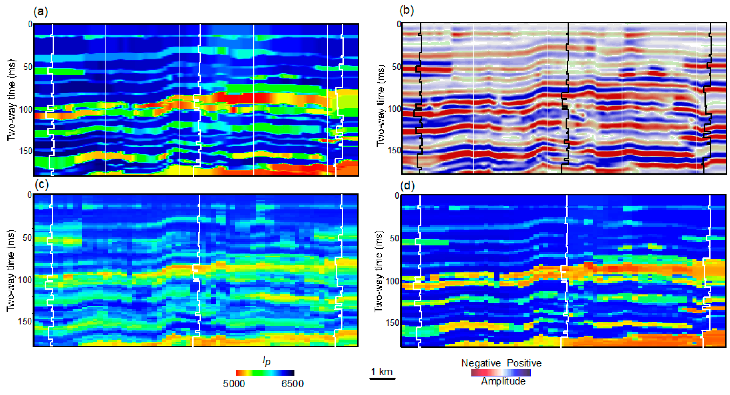
Machine learning (ML) is becoming increasingly important in various fields today. With a high-quality training data set, ML can effectively “assign” or “learn” detailed information about core and wireline-log characteristics—both facies and lithology—into areas between wells. This process relies on a complex nonlinear regrouping of seismic attributes. Model testing has demonstrated this potential (see Figure 8). For instance, in an interbedded formation (Figure 8a), the band-limited seismic responses (Figure 8b) show rounded bed boundaries and often overlook variations in thickness. Although ML can use single-well training data to predict some of these thickness variations, the boundaries remain mostly blurred, indicating improved resolution but still some limitations (Figure 8c). In contrast, a model based on 500 wells conveys much high-resolution information in the predicted section, resulting in sharp boundaries (Figure 8d). These two cases demonstrate the range of improvements expected in practical AI applications. Further studies are needed to reveal the detailed mechanisms behind these processes. ML is poised to significantly enhance thin-bed mapping using seismic data, creating numerous opportunities to explore and develop conventional and unconventional resources.
8. Discussions
1. Always calibrate with well and outcrop information and regional/local geologic model: When interpreting seismic data, we should realize that interpretation is just an approximation of the truth, not necessarily the truth itself. Interpretation is rarely unique and requires verification before being finalized. Therefore, we should always verify and calibrate seismic interpretation with well and outcrop observations; in areas without drilling data or lacking outcrop analogs, a geologic model in adjacent regions or comparable formations should be tested for any interpretational benefits.
2. Push for better integration: How can we enhance seismic sedimentology using current knowledge and technology? There are at least two approaches to consider. We need to publish more models and case studies validating practical workflows and thin-bed indicative attributes to improve our understanding of various depositional systems under different data conditions. Additionally, achieving higher resolution is more than just the responsibility of geophysicists; it requires greater collaboration with geologists. We should build highly integrated research and operational teams to foster this collaboration. Furthermore, we should encourage undergraduate and graduate students in geoscience schools to expand their curriculum by including a wide range of geological and geophysical disciplines.
3. Look forward to the future development of high-resolution geophysics: Recent widespread applications of seismic sedimentology have demonstrated tremendous potential for resource exploration and development across many basins, particularly where seismically thin-beds serve as the dominant reservoirs. However, extracting spatial resolution on stratal slices often involves a trade-off with band-limited data. Closely spaced thin-beds within a seismic event, typically ranging from 5 to 40 meters (λ /4) interval, are challenging to distinguish in vertical sections and horizontal views, leading to potential interpretation confusion. We require next-generation, high-bandwidth acquisition and processing technologies to ultimately address mapping difficulties associated with thin-beds.
9. Conclusions
1. For lithologic and facies mapping using seismic data, “high-resolution” refers to the ability to interpret the top and base of a sedimentary bed with a thickness of λ/4 (typically between 15 and 150 meters) in a vertical view. Additionally, it allows for the detection of beds as thin as λ/80 (ranging from 1 to 5 meters) (spatial resolution) when applying seismic sedimentology from a horizontal view.
2. Among the various choices of attributes and display formats, displaying 90° data and frequency fusion on a stratal slice is considered one of the best workflows for seismic sedimentology.
3. Seismic modeling is essential for verifying and calibrating seismic sedimentological interpretations.
4. Looking ahead, machine learning-based approaches in seismic sedimentology represent the future of this field.
Acknowledgments
The State of Texas Advanced Resource Recovery (STARR) program supported this study. Publication authorized by the Director, Bureau of Economic Geology, Jackson School of Geosciences, The University of Texas at Austin.
Conflicts of interest
The author declares no conflict of interest.
References
- Biddle, K. T.; Schlager, W.; Rudolph, K. W.; Bush, T. L. Seismic model of a progradational carbonate platform, Picco di Vallandro, the Dolomites, Northern Italy. American Association of Petroleum Geologists Bulletin, 1992, 76, 14-30.
- Brown, A. R. Interpretation of three-dimensional seismic data. American Association of Petroleum Geologists Memoir 42, 3rd ed., 1991, 341.
- Castagna, J. P.; S. Sun Comparison of spectral decomposition methods. First Break, 2006, 24, 75-79.
- Dong, Y.; Zhu, X.; Zeng, H.; Bian, S.; Liu, C.; Cheng, K.; Xu, X. Study of seismic sedimentology in Qinan Sag (China). Journal of China University of Petroleum, 2008, 32(4), 7-12.
- Fehmers, G. C.; Höcker, C. F. W. Fast structural interpretation with structure-oriented filtering. Geophysics, 2003, 68, 1286-1293.
- Grossmann, A.; Morlet, J. Decomposition of Hardy functions into square integrable wavelets of constant shape. SIAM Journal on Mathematical Analysis, 1984, 15, 723–736. [CrossRef]
- Johnston D. H., ed. Methods and applications in reservoir geophysics. Society of Exploration Geophysicists, Investigations in Geophysics Series 15, 2010.
- Kallweit, R. S.; Wood, L. C. The limits of resolution of zero-phase wavelets. Geophysics, 1982, 47, 1035-1046.
- Li, C.; Liner, C. Singularity exponent from wavelet-based multiscale analysis: A new seismic attribute. Chinese Journal of Geophysics, 2005, 48, 953–959.
- Li, C.; Liner, C. Wavelet-based detection of singularities in acoustic impedances from surface seismic reflection data. Geophysics, 2008, 73, V1–V9. [CrossRef]
- Lindsey, J. P. The Fresnel zone and its interpretive significance. The Leading Edge, 1989, 8(10), 33–39.
- Liner, C. L.; Li, C.; Gersztenkorn, A.; Smythe, J. SPICE: A new general seismic attribute. 74th Annual International Meeting, Society of Exploration Geophysicists, Expanded Abstracts, 2004, 433–436.
- Mallat, S.; Zhang, Z. Matching pursuits with time-frequency dictionaries. IEEE Transactions on Signal Processing, 1993, 41, 3397–3415.
- Matos, M. C.; Davogustto, O.; Zhang, K.; Marfurt, K. J. Detecting stratigraphic discontinuities using time frequency seismic phase residues. Geophysics, 2011, 76, 1–10. [CrossRef]
- Matos, M. C.; Marfurt, K. J. Inverse continuous wavelet transform “deconvolution.” 81st Annual International Meeting, Society of Exploration Geophysicists, Expanded Abstracts, 2011, 1861–1865.
- Partyka, G.; Gridley, J.; Lopez, J. Interpretational applications of spectral decomposition in reservoir characterization. The Leading Edge, 1999, 18, 353–360.
- Portniaguine, O.; Castagna, J. P. Inverse spectral decomposition. 74th Annual International Meeting, Society of Exploration Geophysicists, Expanded Abstracts, 2004, 1786–1789.
- Posamentier, H. W. Seismic geomorphology and depositional systems of deep water environments: Observations from offshore Nigeria, Gulf of Mexico, and Indonesia (abs.). American Association of Petroleum Geologists Annual Convention Program, 2001, A160.
- Posamentier, H. W. Ancient shelf ridges—A potentially significant component of the transgressive systems tract: Case study from offshore northwest Java. American Association of Petroleum Geologists Bulletin, 2002, 86 (1), 75–106.
- Posamentier H. W.; Dorn, G. A.; Cole, M. J.; Beierle, C. W.; Ross, S. P. Imaging elements of depositional systems with 3-D seismic data: A case study. Gulf Coast Section SEPM.
- Foundation, 17th Annual Research Conference, 1996, 213– 228.
- Schlager, W. The future of applied sedimentary geology. Journal of Sedimentary Research, 2000, 70, 2–9. [CrossRef]
- Sheriff, R.E. Encyclopedic Dictionary of Exploration Geophysics. 3rd Edition, Society of Exploration Geophysicists, 1991, 383.
- Sicking, C. J. Windowing and estimation variance in deconvolution. Geophysics, 1982, 47, 1022–1034. [CrossRef]
- Smith, M. G. P.; Stein, J.; Bertrand, A.; Yu, G. Extending seismic bandwidth using the continuous wavelet transform. First Break, 2008, 26, 97-102.
- Taner, M. T.; Sheriff, R. E. Application of amplitude, frequency, and other attributes to stratigraphic and hydrocarbon determination, in C. E. Payton, ed., Seismic stratigraphy. American Association of Petroleum Geologists Memoir 26, 1977, 301–328.
- Tipper, J. C. Do seismic reflections necessarily have chronostratigraphic significance? Geological Magazine, 1993, 130, 47–55.
- Vail, P. R.; Mitchum, Jr. R. M.; Thompson III S. Stratigraphic interpretation of seismic reflection patterns in depositional sequences, in C. E. Payton, ed., Seismic stratigraphy. American Association of Petroleum Geologists Memoir 26, 1977, 63–82.
- Zeng, H. Ultra-thin, lacustrine sandstones imaged on stratal slices in the Cretaceous Qijia Depression, Songliao Basin, China (ext. abs.), in Society of Exploration Geophysicists Annual Meeting, San Antonio, 2011, 951‒955.
- Zeng, H. Thickness imaging for high-resolution stratigraphic interpretation by linear combination and color blending of multiple-frequency panels. Interpretation, 2017, 5(3), T411–T422. [CrossRef]
- Zeng, H. Improving the resolution of 3-D seismic data. Explorer, American Association of Petroleum Geologists, 2024, 45(9), 44-47.
- Zeng, H.; Henry, S. C.; Riola, J. P. Stratal slicing: Part II. Real seismic data. Geophysics, 1998, 63(2), 514– 522.
- Zeng, H.; Hentz, T. F. High-frequency sequence stratigraphy from seismic sedimentology: applied to Miocene, Vermilion Block 50, Tiger Shoal area, offshore Louisiana. American Association of Petroleum Geologists Bulletin, 2004, 88(2), 153–174.
- Zeng, H.; Xu, Z.; Liu, W.; Janson, X.; Fu, Q. Seismic-informed carbonate shelf-to-basin transition in deeply buried Cambrian strata, Tarim Basin, China. Marine and Petroleum Geology, 2022, 136, 18 p. [CrossRef]
- Zhu, X.; Dong, Y.; Zeng, H.; Lin, C.; Zhang, X. Current status and future of seismic sedimentology in China. Journal of Palaeogeography, 2020, 22(3), 397-411.
Figure 1.
The definition of seismic resolution seen on a synthetic model of a step-wised impedance profile. A zero-phase Ricker wavelet is used. R refers to the reflection coefficient.
Figure 1.
The definition of seismic resolution seen on a synthetic model of a step-wised impedance profile. A zero-phase Ricker wavelet is used. R refers to the reflection coefficient.
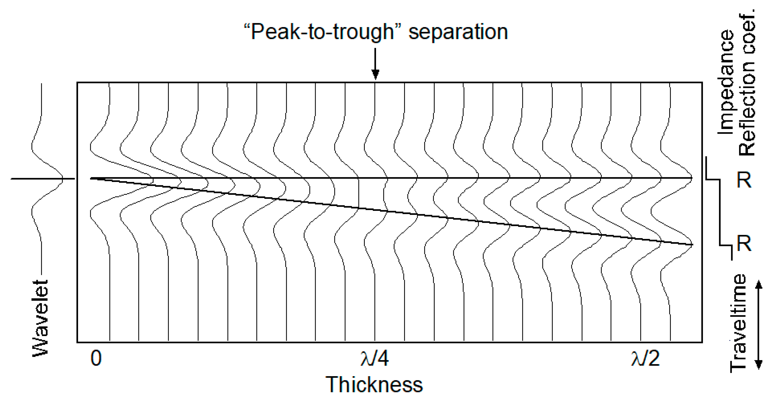
Figure 2.
At λ/4 thickness, maximum amplitude (tuning point) is observed in a synthetic model of a low-impedance wedge encased in high-impedance rock. A zero-phase wavelet is applied. R refers to the reflection coefficient.
Figure 2.
At λ/4 thickness, maximum amplitude (tuning point) is observed in a synthetic model of a low-impedance wedge encased in high-impedance rock. A zero-phase wavelet is applied. R refers to the reflection coefficient.
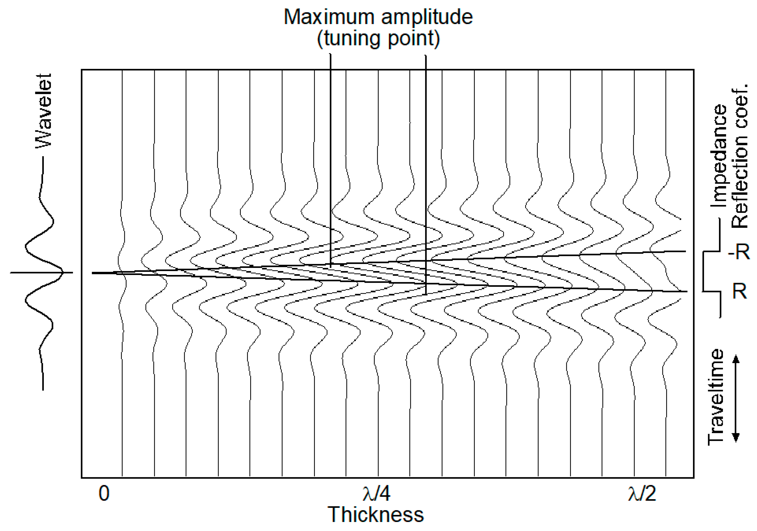
Figure 3.
The result of 90° phase shift of the synthetic model in Figure 2. The central trough is a reasonable estimate of the low-impedance wedge lithofacies.
Figure 3.
The result of 90° phase shift of the synthetic model in Figure 2. The central trough is a reasonable estimate of the low-impedance wedge lithofacies.
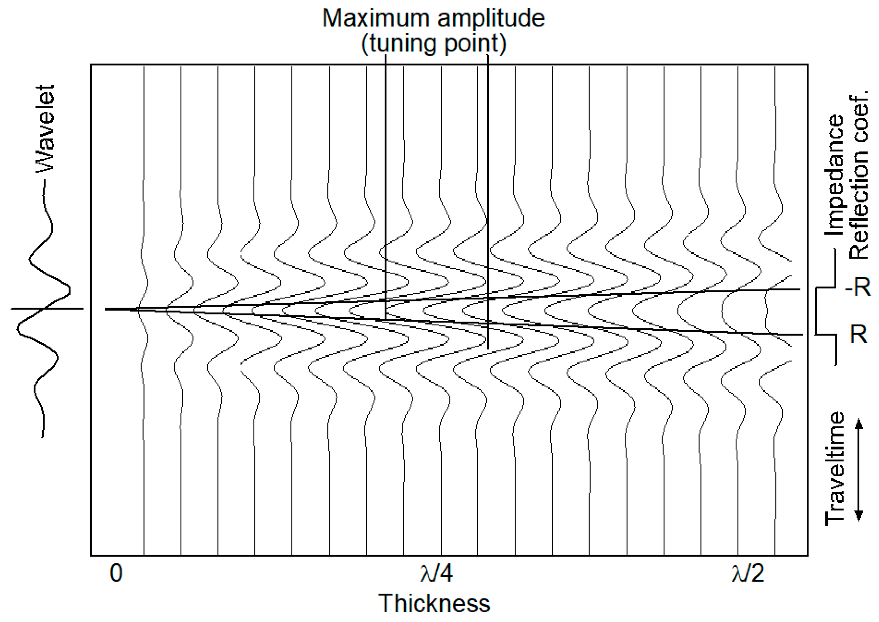
Figure 4.
Frequent fusion can further improve the interpretability of 90° phase data. (a) On a vertical section (labeled SEC) of stacked and migrated data, seismic events (a-g) do not fit the geometry of channel sand bodies. (b) In the same section, using frequency-fused data, RGB events (a-g) roughly fit the geometry of channel sand bodies. (c) On a stratal slice (labeled SS) imaged with stacked and migrated data, channel images (1-7) are mostly blurred. (d) On the same stratal slice with frequency-fused data, channel images (1-7) are more continuous with sharper boundaries and valid thickness definitions.
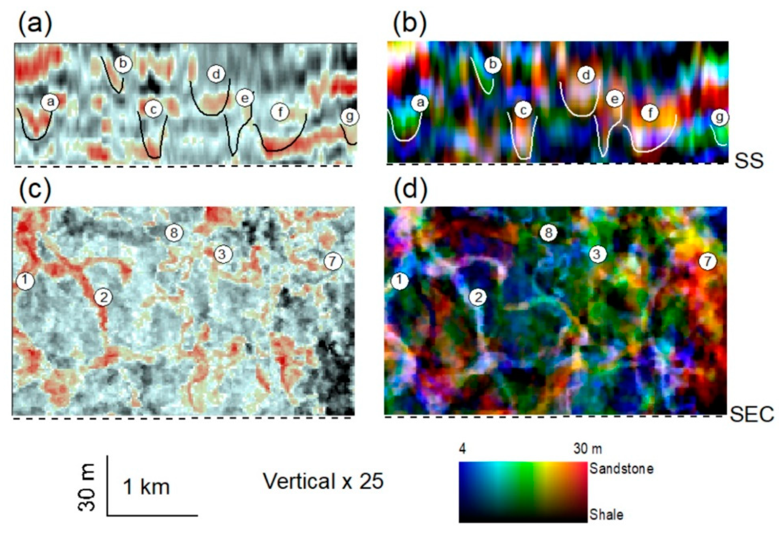
Figure 5.
High-resolution stratigraphic imaging and analysis are achieved by fusing three frequencies from a 90° seismic volume. (a) System tracts and sequence stratigraphy influenced sand thickness, (ranging from 15 to 50 m in the gamma-ray log at the well) and depositional cycles. (b) An RGB blending of 14-, 30-, and 50-Hz iso-frequencies created with MPD is not optimal for stratigraphic imaging. Modified from Zeng (2024).
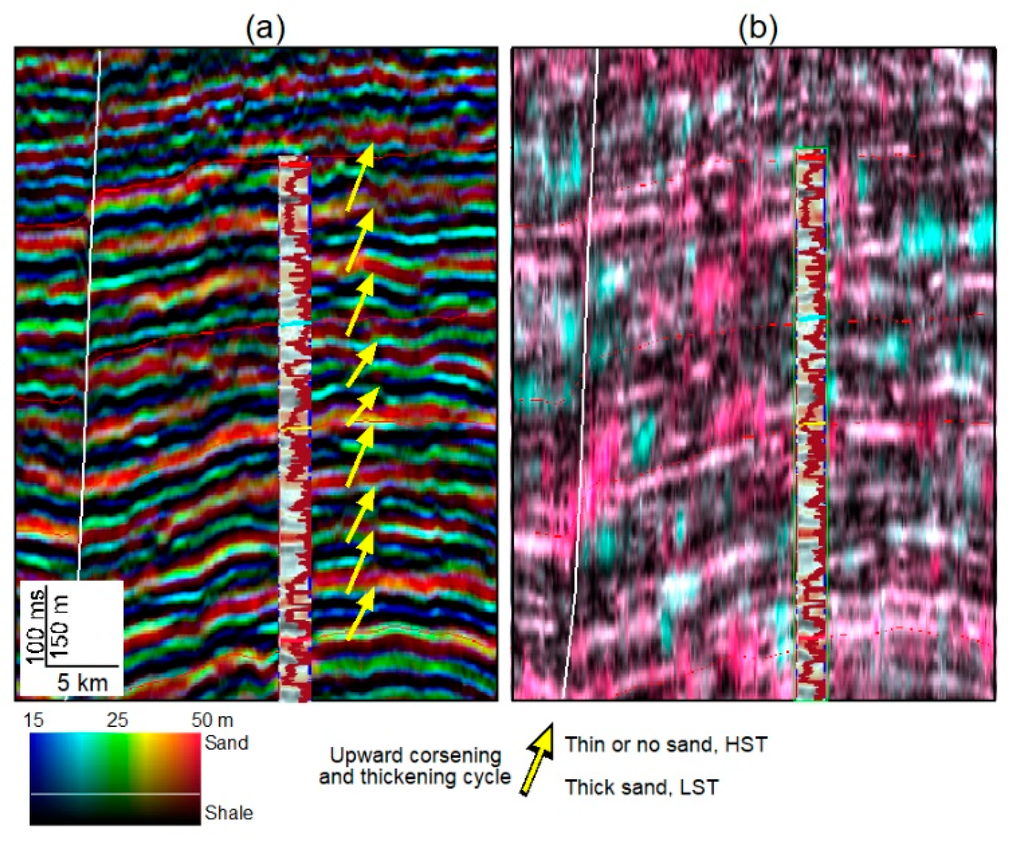
Figure 6.
An optimal spatial resolution (1 m) is indicated by a stratal slice created from a 50-Hz dominant frequency 3D volume in a lacustrine shallow-water deltaic system. The thickness (m) of sandstone measured in gamma-ray logs in wells shows a linear relationship with amplitude. Modified from Zeng (2011).
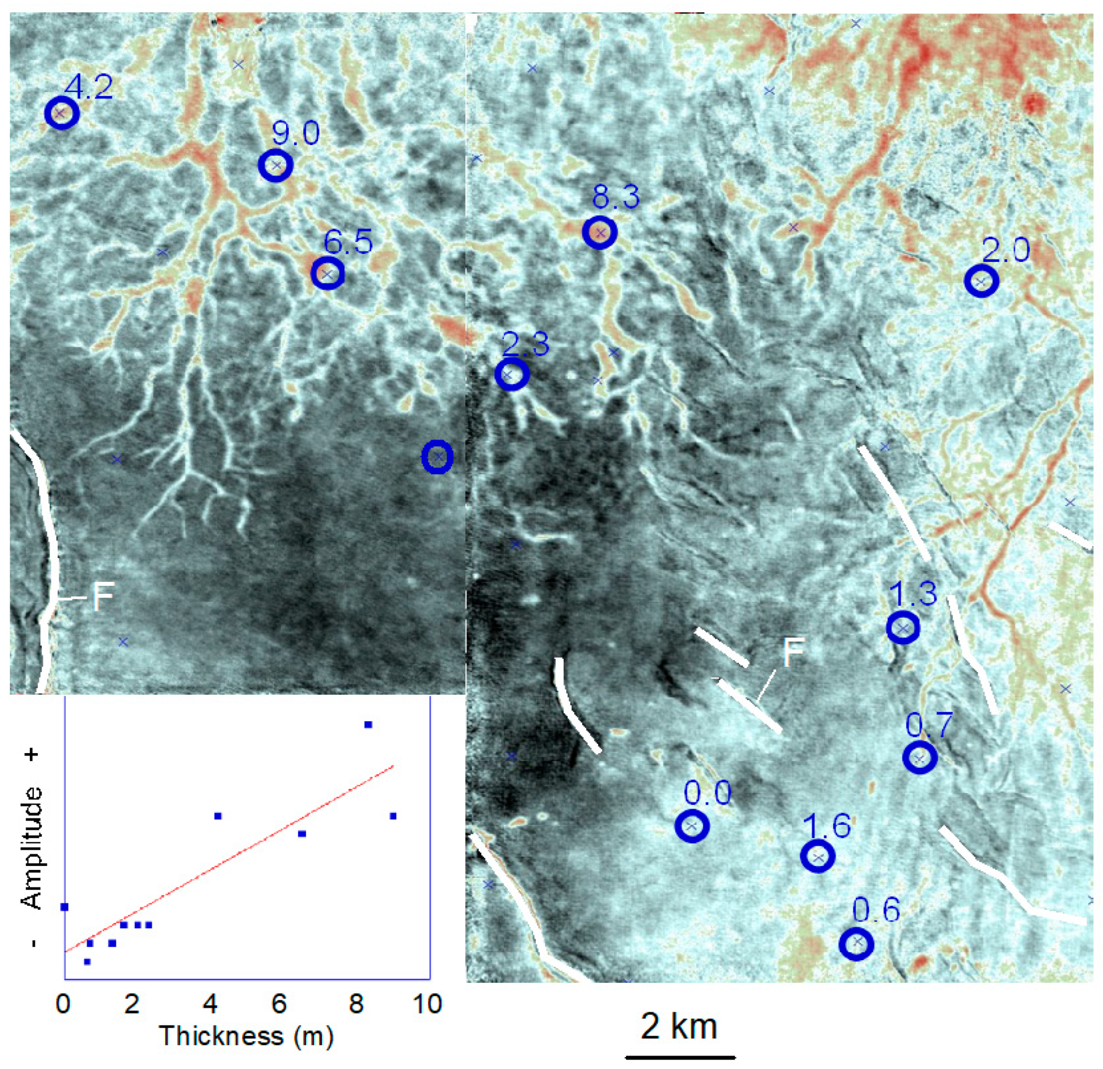
Figure 7.
Thin progradational clinoforms show a discontinuous-chaotic vertical pattern but a clear parallel horizontal pattern. (a) A 3D impedance model of outcrop-based, 50-ms (150 m) thick, progradational sequence. (b) A vertical synthetic seismic section of a 28-Hz wavelet illustrates mostly discontinuous to chaotic reflections. (c) A horizontal amplitude slice showing a parallel pattern perpendicular to the progradation direction. Modified from Zeng et al. (2022).
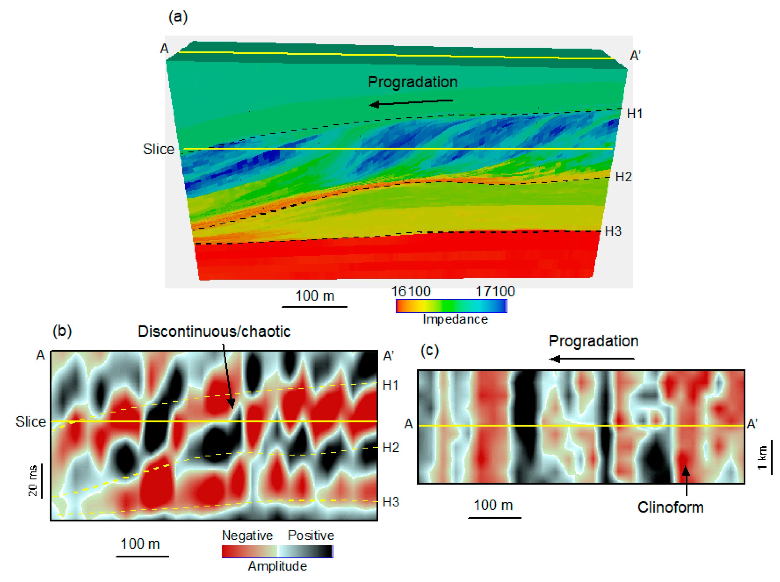
Figure 8.
A test of ML-based inversion workflow. (a) A realistic acoustic impedance (Ip) model (true model) of an interfingered sandstone and shale formation. (b) A 60-Hz Ricker wavelet with a phase shift of 90° was generated from the true model displayed in part (a). This display loses thickness information. (c) The testing results came from a large training data set using one well. The results showed only limited recovery of true thickness variation. (d) Testing results using a 500-well-based large synthetic training data set, which recovers most of the high-resolution details in (a). The logs in the three wells are for blind-testing purposes only. Modified from Zeng (2024).
Disclaimer/Publisher’s Note: The statements, opinions and data contained in all publications are solely those of the individual author(s) and contributor(s) and not of MDPI and/or the editor(s). MDPI and/or the editor(s) disclaim responsibility for any injury to people or property resulting from any ideas, methods, instructions or products referred to in the content. |
© 2024 by the authors. Licensee MDPI, Basel, Switzerland. This article is an open access article distributed under the terms and conditions of the Creative Commons Attribution (CC BY) license (http://creativecommons.org/licenses/by/4.0/).
Copyright: This open access article is published under a Creative Commons CC BY 4.0 license, which permit the free download, distribution, and reuse, provided that the author and preprint are cited in any reuse.


