
Submitted:
14 November 2024
Posted:
18 November 2024
You are already at the latest version
Abstract
The Software-Defined Radio (SDR) technology has been a very popular and powerful prototyping device for decades. It has been applied in either fundamental research or application-oriented tasks. Additionally, the continuing rise of the Internet of Things is needed to validate, process and decode a large number of received signals. This is where SDRs can be a valuable instrument. In this work, we present an open-source software system using GNU Radio and SDRs, which improves the comprehension of the physical layer aspects of Internet of Things (IoT) communication systems. Our implementation is generic and application-agnostic. Therefore, it can serve as a learning and investigation instrument for any IoT communication system. Within this work, we have implemented the open-source DASH7 Alliance Protocol (D7AP). The developed software tool can simulate synthetic DASH7 signals, process recorded data sets, and decode the received DASH7 packets in real time using an SDR front-end. The software is accompanied by three data sets collected in a controlled, indoor and suburban environment. The experimental results reveal that the total packet loss of the data sets is 0%, 2.33% and 16.67%, respectively. Simultaneously, the three data sets have been received by a dedicated DASH7 gateway with a total packet loss of 0%, 3.83% and 7.92%, respectively.
Keywords:
low power wide area networks
; LPWAN
; LoRaWAN
; LoRa
; Sigfox
; DASH7
; GNU radio companion
; Software-Defined Radio
; SDR
1. Introduction
The Internet of Things (IoT) is a concept that has been evolving in the last decade to provide internet connectivity to objects that we use in everyday life. The versatility of these objects knows no limits. They can be generic devices such as bicycles, motors, home appliances, tools of any kind, and devices such as temperature, humidity, air quality or inertial measurement unit sensors. These objects are also usually equipped with extra hardware that constitutes mainly a processing unit and a transceiver for digital communications. Consequently, this hardware will enable the objects to communicate with one another or to send information to the internet [1]. The IoT concept aims to provide an extra layer of intelligence to these objects by enabling remote access. Furthermore, it allows interaction among several objects to achieve a high operational efficiency [2,3]. Accordingly, the IoT concept has been attracting the attention of many industries where automation has a key role. Applications can be found in home and industrial automation, medical aids, energy management, automotive, smart cities, etc.
Moreover, Low Power Wide Area Networks (LPWAN) have emerged to provide the communication means that have enabled the IoT concept. Most LPWAN technologies can, in principle, provide the required internet connectivity to millions or even billions of objects. This communication revolution can be attributed to the LPWAN capability of establishing long-range communication links that go up to several kilometres while using low-power transceivers [4]. Moreover, due to the low production cost, LPWAN transceivers are massively deployed in large-scale environments, i.e., on the scale of cities or even countries.
During the last decades, Software-Defined Radio (SDR) technology has also become a very popular and powerful prototyping tool [5,6]. Before the introduction of the SDR technology, researchers and manufacturers were only relying on custom-made expensive hardware and simulation tools. Although simulation tools can be very powerful in describing any physical behaviour, they can not include all the physical variables that are associated with complex engineering problems. On the other hand, the SDR technology can provide a physical prototype that can be subjected to testing scrutiny. A noticeable trend in recent years is that the SDR technology has been used as a final product for many communication system technologies which is due to the decreasing production costs.
In this paper, we make use of the SDR technology to design the physical layer for LPWAN communication systems. The design steps are generic and can be deployed with any LPWAN standard. However, we have adopted the DASH7 Alliance Protocol (D7A) [7]. This communication standard has been selected to represent IoT communication systems because its specification is freely available [8], and an open-source software stack is ready to use [9]. The proposed SDR implementation of the DASH7 standard has been validated using simulation and experimental analyses. Furthermore, we have provided raw DASH7 signals that were recorded using the SDR front-end in indoor and outdoor environments to test our implementation; these data sets were correctly labelled, and the accurate position of every transmitted signal was reported, which can be used in various applications, including localisation.
In the following section, several LPWAN technologies will be presented, and a brief introduction to the SDR technology will be provided. The DASH7 Alliance Protocol and our SDR implementation are presented in Section 4 and Section 5. In Section 6, we present simulation and experimental results that consolidate our implementation capabilities, which are followed by the discussion about the achieved results in Section 7. Subsequently, conclusions are drawn in Section 8. Finally, several technical appendices are presented to serve as tutorial material to understand common coding and decoding techniques used in telecommunication systems.
2. LPWAN Technologies
Several LPWAN technologies have been introduced over the years. In the following sections, a brief description of several established technologies will be provided. Furthermore, an overview of the key characteristics are depicted in Table 1.
2.1. LoRaWAN
As a small start-up company, Cycleo introduced the LoRa (Long Range) communication network in 2009 [10]. Three years later, the company was acquired by the Semtech corporation [11]. Since that time, LoRa Wide Area Networks (LoRaWAN) have been deployed all over the world to provide long-range and low-power communication for IoT networks [12].
The LoRaWAN physical layer is closed-source and proprietary. It utilises Chirped Spread Spectrum (CSS) modulation in the unlicensed Sub-1 GHz frequency bands [13]. The operational bandwidth can be either 125, 250 or 500 kHz. Moreover, the allowed data rate varies from 300 bits per second (bps) to 50 kbps [14,15]. Accordingly, the characteristics of a LoRa signal, i.e. the carrier frequency, the bandwidth of the signal and the modulation technique, allow LoRa networks to establish communication links up to 15 km in rural areas [2]. Besides that, LoRa sub-GHz has an extension, namely LoRa GHz, which was announced in 2020. This LPWAN technology has the benefit of using the widely used unlicensed GHz Industrial, Scientific and Medical (ISM) band and, therefore, is not subject to duty cycle restrictions. The technology is based on the same CSS technique, but the bandwidths, spreading factors and, therefore, data rates are expanded. Nevertheless, the advertised communication ranges seem to be higher compared to any other technology that is operating in this band [12].
2.2. Sigfox
In 2010, the French startup Sigfox introduced the Sigfox technology, which can serve as an IoT communication network [10]. The Sigfox physical layer is also closed-source and proprietary. It utilises Binary Phase Shift-Keying (BPSK) modulation in the unlicensed Sub-1 GHz frequency bands [10]. Sigfox exploits the Ultra Narrowband (UNB) technology with an uplink of 100 Hz bandwidth. Therefore, Sigfox signals encounter very low noise levels. Consequently, Sigfox gateways have a high receiving sensitivity, and the transceivers consume minimal power. Accordingly, a Sigfox gateway is presumed to handle up to a million connected objects with a coverage of 50 km in rural areas [2]. To achieve this low power consumption and long communication range, Sigfox networks limit the transmission throughput to 100 bps.
2.3. NB-IoT
Narrowband Internet of Things (NB-IoT) technology has been introduced by 3GPP to provide LPWAN services [14]. The NB-IoT standard utilises mobile network features (e.g. user identity confidentiality, authentication, and integrity). It is designed to achieve excellent coexistence performance between Global System for Mobile Communication (GSM) and Long-Term Evolution (LTE) technologies [16]. NB-IoT requires 180 kHz minimum system bandwidth for both downlink and uplink. Therefore, a GSM operator can replace one GSM carrier of 200 kHz to NB-IoT. An LTE operator can deploy NB-IoT inside an LTE carrier by reallocating one of the Physical Resource Blocks (PRBs) of 180 kHz to NB-IoT.
NB-IoT utilises BPSK and Quadrature Phase Shift-Keying (QPSK) modulations at a frequency band of 700 MHz, 800 MHz and 900 MHz. Consequently, NB-IoT can provide a communication link in rural areas up to 10 km [10].
2.4. DASH7
DASH7 is an open-source standard for wireless communication. It provides ultra-low power and mid-range communication connectivity that is suitable for IoT applications. A DASH7 network can establish a communication link up to 5 km. Therefore, DASH7 is technically not an LPWAN technology. It is worth noting that some review papers are classifying the DASH7 standard as an LPWAN technology [17].
According to the DASH7 Alliance Protocol (D7AP) specification, the DASH7 physical layer utilises Gaussian Frequency Shift-Keying (GFSK) modulation in the unlicensed Sub-1 GHz frequency bands. Moreover, DASH7 signals can be categorised into three channel classes with different parameters. The Lo-Rate class has an operational bandwidth of 25 kHz and a data rate of kbps, the Normal class with an operational bandwidth of 200 kHz and a data rate of kbps and finally the Hi-Rate class which has an operational bandwidth of 200 kHz and a data rate of kbps [5,7,18]. Consequently, the DASH7 physical layer characteristics, i.e. the carrier frequency, the signals’ operational bandwidth and the minimal transmission power, are similar to the aforementioned LPWAN technologies.

Table 1.
An overview of the LPWAN technologies physical layer characteristics.
| Operating frequency (MHz) |
Bandwidth (kHz) |
Range (km) |
Data rate (kbps) |
|
|---|---|---|---|---|
| LoRaWAN | 433/868 (EU) | 125/250/500 | 5 (urban) | 0.3 - 50 |
| Sub-1 GHz | 915 (US) | 20 (rural) | ||
| LoRaWAN | 2,400 | 203/406 | 0.5 (urban) | 0.595 - 253.91 |
| 2.4 GHz | 812/1625 | 10 (rural) | ||
| Sigfox | 868 (EU) | 0.1 (UL) | 10 (urban) | 0.1 (UL) |
| 915 (US) | 0.1 (DL) | 40 (rural) | 0.6 (DL) | |
| NB-IoT | Licensed | 180 | 1 (urban) | 150 (UL) |
| LTE bands | 10 (rural) | 127 (DL) | ||
| D7AP | 433/868 (EU) | 25/200 | 1 - 2 (urban) | 9.6/55.6 |
| 915 (US) | 5 (rural) | 166.7 |
3. SDR Technology
The SDR technology allows software modules to run on a generic hardware platform used to implement radio functions. By combining an SDR front-end with a software platform, the user can exploit the SDR technology to rapidly prototype communication systems, including physical layer design, recording and playback of signals, signal intelligence, algorithm validation and more. In the following section, we provide a brief introduction to the main aspects of the SDR technology.
3.1. SDR Architecture
Nowadays, various Commercial-Off-The-Shelf (COTS) SDRs are available to use. These SDRs vary in terms of cost, operational modes i.e. transmitting, receiving or simultaneously, operating bandwidth, frequency bands and the amount of coherent RF channels. Table 2 provides a brief comparison among several commercial SDR front-end units. In the following sections, the reception and transmission operations that are handled by the SDR front-end are briefly introduced.
3.1.1. SDR Transmission Mode
During the transmission process, the baseband In-phase and Quadrature (I/Q) samples are synthesised by the host computer and fed to the onboard FPGA of the SDR at a specified sampling rate. The FPGA interpolates the data to a higher sampling rate using a digital up-conversion (DUC) process. Thereafter, it converts the signal to the analogue domain with a digital-to-analogue converter (DAC). The signal will be mixed with a specified carrier frequency signal that is generated by a local oscillator (LO). After this stage, the signal is amplified and ready to be transmitted [19].
3.1.2. SDR Receiving Mode
The first stage in the reception process is the down-conversion of the received signal by mixing the incoming signal with a LO. In this way, the received signal is converted from the Radio Frequency (RF) domain to the Intermediate Frequency (IF) domain. The IF signal is then represented by I/Q-components. Afterwards, the intermediate I/Q components will be sampled by an analogue-to-digital converter (ADC). The digitised I/Q data follows parallel paths through a digital down-conversion (DDC) process which mixes, filters and decimates the input signal to a user-specified sampling rate. The down-converted samples will then be sent to the host computer. Both transmitting and receiving operations are depicted in Figure 1.
3.2. GNU Radio
GNU Radio is a free and open-source software development toolkit that provides signal processing blocks to implement software radios [20]. It can be used with COTS SDRs or in a simulation mode. it can be used to write applications, to receive data out of digital streams or to push data into digital streams, which can be transmitted using specific hardware. GNU Radio contains a variety of blocks such as filters, channel coders, synchronisation elements, equalisers, demodulators, decoders and many other elements that are typically found in software radio systems. These elements are readily available as software blocks. More importantly, it includes a method of connecting these blocks and then manages how data is passed from one block to another. Adding extra DSP functions can be achieved with the use of Embedded Python blocks. These blocks allow the implementation of custom Python code.
Since GNU Radio is software, it can only handle discrete data. Usually, I/Q baseband samples are the input data type for receivers and the output data type for transmitters. SDRs are then used to shift the signal to the desired centre frequency. However, within GNU Radio, any data type can be passed from one block to another, e.g., bits, bytes, vectors, integers, real and complex numbers. When creating new applications in GNU Radio, they are primarily based on Python. Nonetheless, the performance-critical signal processing path is implemented in C++ using processor floating-point extensions. Thus, the developers can implement real-time, high-throughput radio systems in an easy-to-use environment.
3.3. In-Phase and Quadrature Data
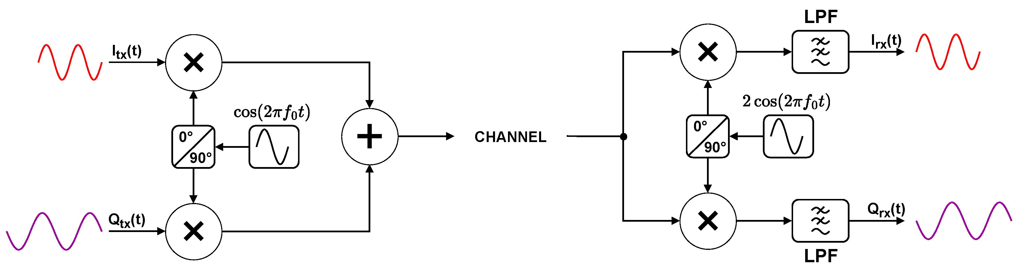
The use of In-phase and Quadrature (I/Q) data is a key concept when working with SDRs. I/Q data is a mathematical complex representation of the transmitted (or received) baseband signal. In this way, I/Q data describes the variations in the amplitude and phase of a signal. An I/Q signal can be represented as two orthogonal signals which form a new waveform. The creation of this new waveform is achieved by using a quadrature modulator, see Figure 2. The two real data signals at the transmitter end can be written as follows:
Combining the two components leads to:
At the receiver end, the in-phase and quadrature components can be recovered as follows1:
By using a low-pass filter (LPF), the high-frequency components, i.e., term two and term three in Equation (4) and Equation (5) are removed, and the in-phase component i(t) and quadrature component q(t) can be recovered at the receiver.
Figure 2.
Concept of an in-phase and quadrature modulator and demodulator.
4. DASH7 Communication System
Before explaining the implementation of our communication system, we first look into several important DASH7 system parameters of the physical layer to obtain a deeper understanding. These parameters are described in the following sections and are defined by the DASH7 Alliance [21].
4.1. Air Interface
4.1.1. RF Channels
As mentioned earlier, the DASH7 communication standard operates in the unlicensed sub-GHz frequency spectrum. The RF band that is available to use depends on the geographical region from where devices are operated. DASH7 supports the 433 MHz, 868 MHz and 915 MHz bands. These bands with their specific channel indexes and frequencies are found in Table 3.
4.1.2. Channel Classes
To avoid signal collisions, the DASH7 protocol divides the specific spectrum band into several channels. Therefore, the DASH7 protocol defines three channel classes that represent the data rates that can be used. These are the Lo-Rate, Normal-Rate and Hi-Rate data rates. Each channel class defines a certain symbol rate, modulation index, frequency deviation and occupied bandwidth [21]. These parameters as displayed in Table 4.
Each channel is defined by an index specifying its start frequency relative to the start of the DASH7 operating frequency band. The centre frequency expressed in Megahertz (MHz) of each channel can be calculated as:
where b and d are the start frequency of the band and the channel index as shown in Table 3, while c is the channel spacing of the selected channel class, which can be found in Table 4.
4.1.3. DASH7 Modulation Scheme
The DASH7 protocol adopts the widely used Frequency-Shift Keying (FSK) modulation scheme with a Gaussian pulse shape filter for the transmitted samples (hence, this modulation is referred to as GFSK). Accordingly, the transmitted waveform can be presented as follows:
where A is the transmitted signal’s amplitude and is the angular phase which can be expressed as follows:
for an FSK signal is:
where a is 1 or -1 and represents the transmitted bit value. L is the number of transmitted bits, and is the shape filter response of the transmitted signal (i.e. for GFSK, the is a Gaussian filter response). Finally, h is the modulation index, and can be expressed as follows:
where is the peak frequency deviation and is the data rate.
In general, GFSK has a higher spectral efficiency compared to FSK. The Gaussian pulse shaping filter smooths the symbol transitions and, therefore, is more bandwidth efficient because it reduces the amount of sidelobes. In this way, it also reduces Inter-Channel Interference (ICI). The effect of FSK and GFSK modulated signals can be seen in a two-dimensional and three-dimensional view in Figure 3 and Figure 4, respectively. The energy is much more spread in the frequency domain when no pulse shaping is applied, whereas the energy is more concentrated when a Gaussian pulse shaping step is implemented.
The spread of a Gaussian-shaped symbol is defined by the bandwidth-to-symbol time product (BT), which, in essence, defines the curvature and amplitude of a symbol in the time domain. This is the product of the duration of a symbol and its spectral width. Its value lies between 0.1 and 1. If the BT has a small value, then the symbol is smeared in the time domain, and therefore, less bandwidth is required. However, it increases the chance of ISI to occur. When the BT product is high, the shape of the curve is closer to a rectangular shape in the time domain. This indicates that there is a lower chance of ISI, but it requires a much higher bandwidth. Therefore, a good trade-off needs to be found. For the executed measurements, a BT of 0.5 was used.
4.1.4. Gaussian Minimum-Shift Keying
When using the Hi-Rate channel class, there is a slight difference compared to the other channel classes. The modulation scheme changes from GFSK to Gaussian Minimum-Shift Keying (GMSK). This is a form of Continuous-Phase Frequency-Shift Keying (CPFSK) [22]. This means that the phase continuity between alternating symbols is maintained. To be more precise, there are no phase discontinuities between symbols observed because the frequency or tone changes happen at the carrier zero crossing points. This is because the frequency difference between the logical 0 and the logical 1 of GMSK is equal to half the data rate. The modulation index for the Hi-Rate channel class is 0.5. This is the smallest value achievable while maintaining orthogonality. In general, GMSK has a higher spectral efficiency than GFSK.
4.2. Packet Structure
Every DASH7 packet is preceded by a power ramp-up and succeeded by a power ramp-down, which is used to meet the band stop channel requirements. The power ramp-up is the time that is needed before the first symbol transmission. This means that the carrier frequency is ramped from idle power to transmit power and settles to a stable state. The reverse operation occurs when ramping down. If this ramp-down is too fast, a part of the encoded frame might be affected, and therefore, the packet can become unrecoverable. Typically, these ramps have a period of 8 symbols but can go up to 32 symbols.
When looking into the Data Link Layer of DASH7, we see two types of frames defined: background frames and foreground frames. Background frames have a static payload size of six bytes. These frames are used to send broadcast messages, which are applied for ad-hoc group synchronisation. Foreground frames can have a length of up to 256 bytes and are used for data requests or contain data.
The preamble is an unencoded static structure of alternating binary symbols starting with ’1’ and can have a variable length of up to 64 bits. This is used to settle the receiver by calibrating its data rate circuits. The DASH7 specification defines a typical preamble length of 32 bits for the Lo-Rate and Normal-Rate class while recommending 48 bits for the Hi-Rate channel class [23].
The sync word is an unencoded structure of 16 binary symbols used to identify the start of the payload. The physical layer supports two sync word classes which depend on the type of frame that is used. Background frames use Sync Word Class 0, while foreground frames use Sync Word Class 1. A second categorisation that makes up a specific sync word is the applied type of encoding. It can be seen from Table 5 that only Coding Scheme 0 (CS0) and Coding Scheme 2 (CS2) are used. In future releases, this can be extended with two additional coding schemes.
Finally, the payload field, which can have a length between 5 and 256 bytes, contains at least a length byte, a subnet byte, a control byte (CTRL), the packet data and two Cyclic Redundancy Check (CRC16) bytes. The CRC operation is applied only to the payload before the encoding process. Its operation is extensively explained in Appendix A. Furthermore, the payload is the only encoded part of the packet. This encoding step is achieved with a PN9 code or a combination of a PN9 code and -Forward Error Correction Code (FEC), which are described in Appendix B and Appendix C. Figure 5 shows the general composition of a DASH7 packet.
5. DASH7 Communication System Implementation
In this section, we present the implementation of our communication system using SDR technology. To represent the communication system more conveniently, we divide it into a transmitting and a receiving process. Subsequently, we create separate sections. The details of both methods will be thoroughly explained in the following sections.
5.1. The Transmitting Process
This process constitutes three steps: a data formatting process, a symbols to waveform conversion and a modulation step. These operations will be discussed in the following sections.
5.1.1. Data Formatting
This process foresees the correct format for the packet as specified by the communication protocol [21]. The DASH7 protocol specifies that the packet starts with a preamble followed by a sync word and, finally, the payload containing the actual data message. Furthermore, the payload begins with one byte that specifies the length of the payload and ends with two CRC16 bytes, which are used as a bit error check. Finally, the payload data needs to be whitened using a PN9-code. The CRC and the PN9 calculations are presented in Appendix A and Appendix C, respectively. Optionally, a -FEC can be applied before the PN9 coding operation, but this depends on the used coding scheme. A summarised operation of the FEC process can be found in Appendix B.
Figure 6 shows the GNU Radio implementation of the DASH7 data formatting step. The Parameter-blocks contain all the required variables to create a synthetic DASH7 packet. The bytes in our implementation are represented as decimal numbers. For instance, the decimal number 170 represents a byte of the preamble data, i.e. “10101010”. Accordingly, you can add the decimal number 170 for every eight bits of preamble data. On the other hand, the two bytes of the sync word represent the value depending on a specific Sync Word Class and selected Coding Scheme as shown in Table 5. Sync Word Class 0 is used for background frames, while Sync Word Class 1 is only used for foreground frames, which are defined at the data link layer. As for the payload, in our implementation, we have created the CRC16_and_PN9 function, which is a custom Python Module-block. This function is applied in the Coded_Packet parameter block. The main task of this function is to add the length byte of the payload at the beginning and the two CRC16 bytes at the end of the payload. Afterwards, encode the entire payload with the PN9 code. Therefore, the total length of the coded packet is always the length of the payload plus three bytes.
The data formatting box in Figure 6 exploits three Vector sources and a Multiplexer-block. The vector sources are dedicated to the preamble, the sync word, and the payload data. Subsequently, the Binary to symbols box converts each bit into a series of bytes and creates symbols by mapping these values. The 0b is represented by -1, and the 1b is represented by 1. The Throttle-block has been added to control the throughput of the data flow. In this case, we transmit a Lo-Rate DASH7 signal with a symbol rate of kbps. The Virtual Sink-block, in the flowgraph, is used for organisational purposes. Note that the Virtual Sink needs to be linked with a Virtual Source so that the data flows between the sink and the source. The complete transmitted packet is presented in Figure 7. The figure clearly shows the preamble data followed by the sync word and the whitened payload.
5.1.2. Symbols to Waveform Conversion
In the previous section, the complete DASH7 packet has been formatted and converted to symbols. In this section, the symbols, see in Equation (9), will be converted to a waveform. Consequently, every symbol will have a transmission time. Therefore, a single symbol will be represented by multiple samples2.
The process of converting an individual symbol into multiple samples is called upsampling, and the factor that controls this conversion is called the samples per symbol (SPS) factor. Consequently, a larger SPS value will improve the modulation process but at the same time will require a higher sample rate, e.g. the Lo-Rate DASH7 signals’ bit rate is kbps if the SPS is set to 100 this will lead to a sample rate of 960 kbps. After selecting the proper SPS, the pulse shape of the waveform should be specified. When the samples are represented by uniform values, the waveform of these samples will have a rectangular pulse shape. Nevertheless, the rectangular pulse shape is not commonly used in wireless communications due to its large side lobes in the frequency domain. In our application, the pulse shape of the signals will have a Gaussian filter response because DASH7 signals exploit GFSK modulation.
In GNU Radio, we utilise the Interpolating FIR Filter block to simultaneously deploy the upsampling and shape filter processes. This filter creates a Finite Impulse Response (FIR) filter that performs the convolution in the time domain between the payload symbols and the filter taps which happens after upsampling the bits by the SPS factor in the interpolation process. Consequently, if the taps are set to ones, then the output waveform will have a rectangular pulse shape. However, we have deployed a Gaussian shape filter that is defined by the variable Gaussian_Shape_Filter. This variable exploits the GNU Radio firdes.gaussian(gain, SPS, beta, ntaps) function. The gain and SPS parameters are self-explanatory at this point, while beta is a Gaussian filter parameter ranging between 0 and 1. The parameter beta represents the product between the 3 dB bandwidth of the Gaussian filter and the symbol duration, i.e. BT where B is the bandwidth and T is the symbol duration. For instance, if beta equals 0.25, then the Gaussian pulse shape spreads over four symbols. Thus, a smaller beta causes a higher Inter Symbol Interference (ISI) but a compact spectrum. Finally, the ntaps variable specifies the amount of FIR taps. The choice of the number of taps (ntaps) is a trade-off between the filter performance and computational cost. A long tap line will ensure a compact signal bandwidth and good phase and amplitude responses for the signal of interest. A more expanded description regarding FIR-filter design can be found in [24]. In our implementation, the ntaps parameter is equal to the SPS parameter because we usually deploy a high SPS factor. The implementation can be seen in Figure 8. We apply an Automatic Gain Control-block (AGC) to the output of the Interpolating FIR filter-block to obtain a more normalised signal after the pulses have been amplified and shaped.
The generated waveform is depicted in Figure 9. This signal is obtained by upsampling, pulse shaping, and gain control of the mapped symbols. This baseband waveform can now be modulated.
5.1.3. Baseband Modulation
To implement the GFSK modulation in the digital domain, the integration in Equation (8) will be substituted by a summation of calculations as follows
where T is the sampling interval, i.e. the reciprocal of the sampling rate. If we consider the following:
then
leads to
The Z-transform of Equation (14) can be expressed as follows:
which leads to the transfer function,
Equation (16) is the single pole difference equation of an Infinite Impulse Response (IIR) filter, which can be implemented in a straightforward manner in GNU Radio.
Figure 10 shows the FSK modulation flowgraph. First, the signal is multiplied by the factor and the modulation index. Afterwards, the integration process will be conducted using the IIR filter. The Feed-forward and the Feedback Taps control the behaviour of the IIR filter. For the single pole IIR filter, the feedback taps need to be (1, -1), as shown in Equation (16). However, the Feed-forward Taps can vary based on the deployed integrator type. Several integration types can be performed: 1) rectangular integration, where the area under the curve is assumed to be flat; 2) trapezoidal integration, where the area under the curve is assumed to be triangular; and 3) the Simpson’s rule integration, where the area under the curve is assumed to be an arc [25]. To implement this rectangular integration, we use taps that are equal to 1. For trapezoidal integration the taps will change to . Finally, for Simpson’s rule integration, it becomes more complex, and the taps will be set to .
The Feedback Taps should be (1, -1) for the rectangular and trapezoidal integration. However, for the Simpson rule, this will be (1, 0, -1). In general, if the SPS factor is high, the rectangular integration will suffice. The baseband modulated signal is sent to the SDR front-end. On that front-end, the signal will be sent through a DAC and eventually mixed to the needed RF frequency, followed by an amplification stage. Figure 10 depicts the implementation of the rectangular integration in GNU Radio, which generates a modulated baseband signal. The output of this flowgraph in the frequency domain is shown in Figure 11. In the plot, there are two distinct peaks noticeable at kHz and kHz, which are the “space” and “mark” tones used by the Lo-Rate DASH7 channel class.
The upsampling process and shape filter process in GNU Radio, which is achieved with an interpolating FIR filtering.
5.2. The Receiving Process
The receiving process is, in essence, the opposite operation of the transmission process. It comprises four steps: reception, demodulation, time synchronisation, and decoding.
5.2.1. Reception
The reception of a signal while using an SDR happens when the user tunes the local oscillator to or close to the frequency of interest. For FSK modulation, the centre frequency of the SDR front-end needs to be tuned to the same centre frequency of the FSK waveform. Accordingly, any deviation in the frequency between the front-end and the received modulated signal will result in a detection error and can cause a high bit error rate (BER).
In our implementation, the frequency of the received DASH7 signal is assumed to be known by the receiver (in general, in every communication system, this should be the case). Therefore, if the signal is received with an IF frequency, the signal has to be shifted to the centre frequency of the receiving bandwidth. This can be done in GNU Radio by multiplying the received signal with a sinusoidal signal, which has a frequency equal to the IF frequency. Figure 12 presents the flowgraph of the digital mixer operation. The signal source provides a complex single-tone signal with a frequency equal to the IF frequency.
5.2.2. Demodulation
At the receiver, and after tuning the LO at the carrier frequency of the received signal, the received digital baseband signal can be expressed as
where is the received signal’s amplitude. The demodulation process of the received signal can be illustrated as follows:
- Extracting the phase of the baseband signal using a Complex to Arg-block:where k is the digitised time index, and is a constant arbitrary phase due to the phase difference between the transmitter and the receiver.
-
Taking the derivative ofwhere h is the modulation index and is equal to:In order to further decode the packet, we have to:
- Time synchronisation and bits decimation must be performed.
- Payload detection based on the sync word bits.
- To decode the payload data, further data de-whitening and the optional FEC decoding are required.
5.2.3. Time Synchronisation
The demodulated data samples need to be passed through a digital filter that minimises the effects of noise and the effects of Inter-Symbol Interference (ISI). The ISI can be caused when the filtered received pulses overlap. The best filter to maximise the signal-to-noise ratio (SNR) while minimising the ISI is a matched filter (MF). A matched filter has a frequency response whose magnitude matches the magnitude of the frequency response of the transmitter’s shape filter. Accordingly, for DASH7 signals a Gaussian matched filter should be deployed similar to the Gaussian shape filter that is implemented at the transmitter.
Afterwards, the output of the shape filter must be sampled periodically at the symbol rate which is achieved by downsampling the data by the factor SPS, at the precise sampling time instants , where is the symbol interval and is a nominal time delay or timing offset that accounts for the propagation time of the signal from the transmitter to the receiver [26]. Note that in DASH7, the symbol interval is the same as the bit interval. To perform this periodic sampling, we require a symbol clock at the receiver to select the correct symbol from several received samples. The process of extracting such a clock signal at the receiver is usually called symbol synchronisation or timing recovery. Timing recovery is one of the most critical functions that is performed at the receiver of an asynchronous digital communication system. It is important to emphasise that the receiver must know both the transmitted symbol rate (1/) and the time instant to extract the symbol from multiple received samples within each symbol interval .
A clock signal can be extracted from the received data signal. There are many techniques that can be used at the receiver to achieve self-synchronisation. However, in this paper, we have adopted the Mueller and Müller symbol synchronisation method [27]. The details of this method are out of this paper’s scope.
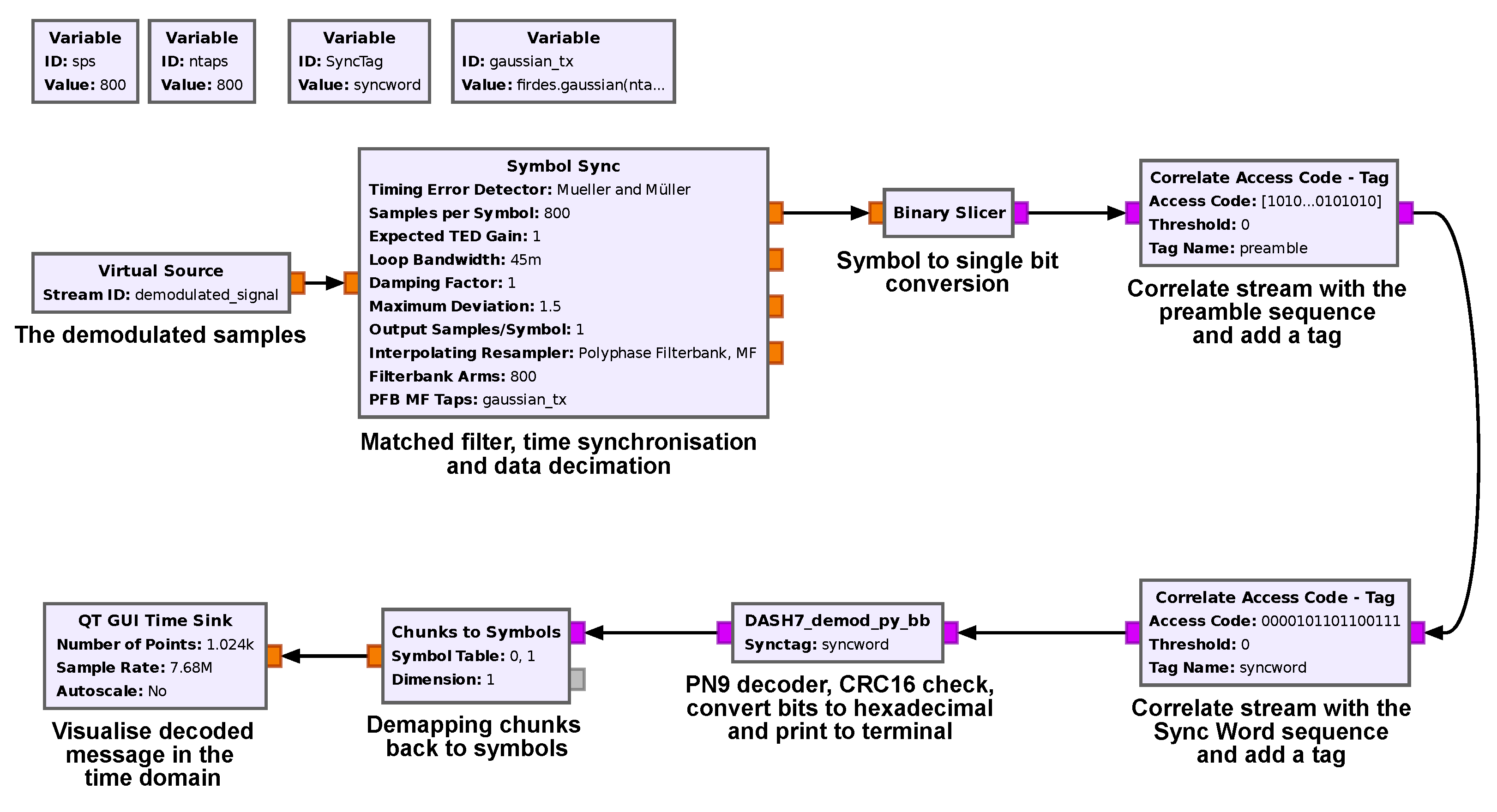
The time recovery process is the first stage after demodulating the received samples, as shown in Figure 14. In GNU Radio, the Symbol Sync-block provides several symbol synchronisation methods, including the Mueller and Müller method; every symbol synchronisation method has its specific parameters. Furthermore, the Symbol Sync allows the definition of any type of match filter when using the Polyphase Filterbank (PF). The input of the Symbol Sync are samples with a sample rate equal to . On the other hand, the output of the Symbol Sync are symbols with a symbol rate of .
5.2.4. Decoding
The first stage after the symbol synchronisation is the binary conversion process. The Binary Slicer-block in Figure 14 converts every negative symbol value to a 0b and the rest to 1b. After converting the symbols to bits, the correlation process will start between the received bits and both the preamble and the sync word. The Correlate Access Code - Tag-block provides a tag that indicates the location of the preamble and the sync word in the data stream. The tags will be exploited by the DASH7_demod_py_bb-block. The py_bb in the block name indicates that the block is implemented using Python code, and it receives and delivers binary data. The DASH7_demod_py_bb-block decodes the received packet. These are the bits after the sync word tag with PN9 sequences. After the decoding process, the block deploys a CRC16 to validate the correct reception of the received packet.
Figure 14.
GNU Radio flowgraph where the demodulated samples are time synchronised and put through a matched filter. After this step, a tag is added when a correlation is found to a predefined preamble and sync word sequence. Finally, the message is PN9 decoded, a CRC check is applied and the output will be printed to the console window.
The output of the decoding process is shown in the GNU Radio Console, which states the number of the packet, the packet length, the calculated CRC check and the message in decimal and hexadecimal form, as can be seen in Figure 15. Note that the payload size of a DASH7 packet is longer due to extra obligatory fields of the other layers.
6. Experimental Setup
The validation of the correct operation of the created software system is achieved by executing several experiments. Therefore, we captured three data sets. The first data set was obtained through a cabled setup. Consecutively, we recorded a data set in an office environment, and another data set was obtained from a suburban environment. The cabled setup served to obtain an optimal condition data set where 10 data transmission for three Lo-Rate channels were recorded. Furthermore, we recorded two wireless data sets i.e. at an indoor and suburban setting. The indoor experiment was conducted on 10 locations, while the outdoor experiment contained 21 predetermined locations. Each data set was tested on three Lo-Rate channels, namely channel 0, 93 and 186. For each location of a wireless data set, we transmitted 60 packets in total. Additionally, we logged the timestamp, channel, payload, RSSI and EIRP from each packet on separate DASH7 gateways.
The measurement setup included six B-L072Z-LRWAN1 STM32 LoRaWAN Discovery Boards and an Ettus Research USRP B210 SDR. Three of the development boards acted as DASH7 nodes or transmitters operating at different Lo-Rate channels. At the receiving end, three boards were configured as DASH7 gateways, where the incoming packets were demodulated and logged. The boards were programmed with the use of the Sub-IoT-Stack, which contains a full, open-source software stack of the DASH7 Alliance Protocol [9]. The nodes use the push communication model and transmit DASH7 messages, i.e. foreground frames with a configurable payload, channel, gain and encoding scheme. Additionally, we used an SDR to record the received data from the DASH7 nodes. This data was fed to the created GNU Radio flowgraph. A brief overview of the measurement setup is depicted in Figure 16. The used software and flowgraphs, accompanied by the recorded data and specifications, are published on Zenodo [28]. A more concise overview of the work can be found at [29].
For the data recording and multi-channel implementation, we used GNU Radio version 3.10.1.1 on a Linux machine. The flowgraphs were created using readily available blocks and Python snippets, making the conversion to older or newer GNU Radio versions more straightforward. The recorded data sets use the Signal Metadata Format (SigMF). This format describes the recorded digital signals with metadata in a JSON format, making it easier to validate and interpret the data during post-processing.
For the cabled measurement, the setup deviates slightly from the wireless setups. We connected the DASH7 node, dedicated channel gateway and SDR through coaxial cables as shown in Figure 17. The DASH7 node is equipped with a 40 dB attenuator and RF-splitter to guide the signal equally to the SDR and DASH7 gateway. Figure 18 depicts the indoor measurement environment. The 10 TX locations are shown as green indicators on the map while the receiving setup, i.e. the SDR and DASH7 gateways are positioned at the red RX indicator. Figure 19 shows the map of the suburban measurement environment. The DASH7 gateways and SDR are positioned at the red pointer while the TX locations are shown in green. One location is shown in blue which is location 21. At this location, there was Non-Line-of-Sight, and no packets were received, as can be seen in Table 6.
7. Results and Discussion
We validated the proper working of the created software by using a cabled setup. The transmitted signals were attenuated with 40 dB. This attenuated signal was split, causing an extra 3 dB attenuation. In this way, the signal was distributed to the dedicated DASH7 gateway and the SDR simultaneously. During 10 measurements per channel, we observed received signal strengths between 21 dB and 22 dB. Subsequently, all packets were recovered at the gateway and from the recorded data.
The obtained results of the indoor and outdoor experiments can be found in Table 6 and Table 7, respectively. We find that the cabled setup has no packet loss at all at the DASH7 gateways and while using recorded data in the receiver flowgraph. However, we observe that the indoor and outdoor experiments do have more packet loss both at the gateway and in GNU Radio. Subsequently, we see that the results of the indoor experiments are better compared to the outdoor data set. The reason for this higher packet loss in the outdoor environment is due to multipath effects, NLOS scenarios and changes in distance between the transmitting location and receiver setup. We also believe that we have reached the limit of the maximum distance of DASH7. It is found that the dedicated DASH7 gateways have occasionally a hard time detecting and decoding the packets properly. We also observe that packet loss tends to occur more often when the mean RSS is equal or lower than dB, however, this is not always the case. We believe this is due to the received signal being close to or even below the noise floor.
For the outdoor data set, we find that packets are received even at a distance of 1180 m which is within the expectations. Location 21 was a worst-case location with no line-of-sight while located at the furthest location.
Eventually, we find that there is less packet loss at the DASH7 gateways compared to the post-processed data in GNU Radio of the indoor data set. The findings for the outdoor data set are slightly different. At certain locations and channels, the software processing outperforms the DASH7 gateways. But in other cases, it performs equal or worse. There are diverse factors that can explain the cause of it. Firstly, multipath, noise and other signals such as LoRa were randomly seen within the data set, which affects the transmitted signals and, therefore, can explain partially the packet loss. Also at channel 0, other signals were observed occasionally. Another reason why the gateway outperforms the SDR recordings is due to sensitivity. It is found that the receiver sensitivity of the B-L072-LRWAN1 board is dBm. The sensitivity of the applied SDR is not advertised and depends on multiple factors. However, we believe the sensitivity of the SDR is worse taking into account the large bandwidth compared to a dedicated, small bandwidth device.
Another explanation for the increased data loss is due to time variances between the packets within one recording. We observed that these dynamic time variances between consecutive packets were between 1 ms and 2 ms. This causes phase shifts in comparison to the locked frequency and phase of the local oscillator, which causes the intermediate frequency to be affected by each received packet. We observed that more or even other packets were decoded successfully by changing the phase offset of the local oscillator.
Another observation within the recordings was a recurring static frequency deviation of about kHz which needed to be adjusted at the first mixing stage in the receiver flowgraph. This is a Centre Frequency Offset (CFO) which is caused by the frequency deviation of the Temperature Compensated Crystal Oscillator (TCXO) of the B-L072-LRWAN1 boards which operates at 20 MHz. This TCXO provides a clock signal to the SX1276 transceiver chip and is used by the DASH7 transmitters and gateways. According to the datasheet, these crystals have a deviation of two parts per million (ppm) [30].
8. Conclusion
In this work, we have presented a communication system based on the DASH7 Alliance Protocol by utilising GNU Radio and Software Defined Radios. The complete communication system works in simulation which makes the software suitable as a learning, analysis and validation tool for DASH7 packets. Furthermore, the demodulation system has been deployed and examined in a cabled setup and in an indoor and outdoor environment. The obtained data sets are open-source and can be consulted on Zenodo. The cabled setup shows that the software is performing sufficiently, while the indoor and outdoor experiments show severe packet loss, which is also observed at the DASH7 gateways. This is due to the nature of field experiments and is caused by multipath effects and varying (N)LOS conditions. Nevertheless, certain optimisations can be done to decrease the packet loss within the software.
In future work, we see several software optimisations. Currently, a lot of parameters are defined statically, which restricts the abilities of the software. To make the system more robust, we need to implement certain DASH7-specific parameters dynamically. These parameters involve correlation with a varying length of the preamble, varying Sync Word Classes and channel classes. When taking these parameters into account, other system parameters need to be changed dynamically as well, for example, filter and gain blocks. Lastly, it is needed to implement the -FEC technique.
On the level of digital signal processing, we find a few shortcomings in the current implementation. Firstly, an automatic Centre Frequency Offset compensation block needs to be created. Secondly, the mixing stage of the demodulator should be improved to a self-centring technique. In this way, the signal is centred at baseband level automatically meaning that it does not matter on which specific channel a signal is received. Thirdly, a phase offset measuring step and phase compensation step need to be added while maintaining the mixing stage. Furthermore, the implementation for Normal-Rate and Hi-Rate channel classes needs to be implemented and validated. Penultimately, the dynamical detection of the used Sync Word Class and coding scheme for a certain packet should be implemented. Finally, the implementation of loading a configuration file containing several DASH7 specification-specific parameters can make the system more dynamic and less error-prone.
Data Availability Statement
The data set presented and used in this study is openly available at https://doi.org/10.5281/zenodo.10961311 (accessed on 10 September 2024).
Acknowledgments
This article is a revised and expanded version of a paper entitled Implementation of a Multi-Channel DASH7 IoT Communication System for Packet Investigation and Validation, which was presented at the 14th Annual GNU Radio Conference which took place in Knoxville Tennessee (USA) from 16 to 20 September 2024.
Appendix A. DASH7 CRC16 Validation
A cyclic redundancy check (CRC) is an error-detecting code commonly used in digital networks and storage devices to detect accidental changes to raw data. Blocks of data entering these systems get a short check value attached, which is based on the remainder of a polynomial division of their contents. On retrieval, the calculation is repeated. When the check values do not match, corrective action can be taken against data corruption. A frame is always terminated by a 16-bit CRC field. Only when the CRC calculation of a received frame matches the supplied value will it be sent to the Data Link Layer, which continues processing the frame. The calculation of the field includes all previous bytes of the frame. For DASH7, the CRC16/CCITT_FALSE polynomial is used. This is expressed as (0x1021 or 10001000000100001B) with an initial value of 0xFFFF. Using this algorithm correctly, the value 0x29B1 will result from the computation of the nine-character ASCII reference string “123456789” (Note: the numbers of the reference string are ASCII encoded, not binary). To compute an n-bit binary CRC, line the bits representing the input in a row, and position the (n + 1)-bit pattern representing the CRC’s divisor (called a “polynomial”) underneath the left-hand end of the row.
Example To make the operation straightforward, we encode a one-byte message with a 3-bit CRC, that uses the polynomial . The polynomial is written in binary as the coefficients; a third-order polynomial has 4 coefficients (). In this case, the coefficients are 1, 0, 1 and 1. The result of the calculation is 3 bits long.
Starting with the message to be encoded: 11001100 This is first padded with zeros corresponding to the bit length (n) of the CRC (add 0 0 0 at the end of the message) and add at the beginning of the message an initial value of n bits (add 1 1 1 at the beginning of the message). The first calculation for computing a 3-bit CRC:
111 11001100 000
101 1 divisor (4 bits) =
——————
010 01001100 000 ← result
The algorithm acts on the bits directly above the divisor in each step. The result for that iteration is the bitwise XOR of the polynomial divisor with the bits above it. The bits not above the divisor are simply copied directly below for that step. The divisor is then shifted one bit to the right, and the process is repeated until the divisor reaches the right-hand end of the input row. The entire calculation is written out below.
| 1 | 1 | 1 | 1 | 1 | 1 | 0 | 0 | 1 | 1 | 0 | 0 | 0 | 0 | 0 |
| 1 | 0 | 1 | 1 | |||||||||||
| 2 | 0 | 1 | 0 | 0 | 1 | 0 | 0 | 1 | 1 | 0 | 0 | 0 | 0 | 0 |
| 1 | 0 | 1 | 1 | |||||||||||
| 3 | 0 | 0 | 0 | 1 | 0 | 0 | 0 | 1 | 1 | 0 | 0 | 0 | 0 | 0 |
| 1 | 0 | 1 | 1 | |||||||||||
| 4 | 0 | 0 | 0 | 0 | 0 | 1 | 1 | 1 | 1 | 0 | 0 | 0 | 0 | 0 |
| 1 | 0 | 1 | 1 | |||||||||||
| 5 | 0 | 0 | 0 | 0 | 0 | 0 | 1 | 0 | 0 | 0 | 0 | 0 | 0 | 0 |
| 1 | 0 | 1 | 1 | |||||||||||
| 6 | 0 | 0 | 0 | 0 | 0 | 0 | 0 | 0 | 1 | 1 | 0 | 0 | 0 | 0 |
| 1 | 0 | 1 | 1 | |||||||||||
| 7 | 0 | 0 | 0 | 0 | 0 | 0 | 0 | 0 | 0 | 1 | 1 | 1 | 0 | 0 |
| 1 | 0 | 1 | 1 | |||||||||||
| 8 | 0 | 0 | 0 | 0 | 0 | 0 | 0 | 0 | 0 | 0 | 1 | 0 | 1 | 0 |
| 1 | 0 | 1 | 1 | |||||||||||
| 9 | 0 | 0 | 0 | 0 | 0 | 0 | 0 | 0 | 0 | 0 | 0 | 0 | 0 | 1 |
Since the leftmost divisor bit zeroed every input bit it touched, when this process ends the only bits in the input row that can be nonzero are the n bits at the right-hand end of the row. These n bits are the remainder of the division step, and will also be the value of the CRC function. The validity of a received message can easily be verified by performing the above calculation again, this time with the check value added instead of zeroes. The remainder should be equal to zero if there are no detectable errors.
| 1 | 1 | 1 | 1 | 1 | 1 | 0 | 0 | 1 | 1 | 0 | 0 | 0 | 0 | 1 |
| 1 | 0 | 1 | 1 | |||||||||||
| 2 | 0 | 1 | 0 | 0 | 1 | 0 | 0 | 1 | 1 | 0 | 0 | 0 | 0 | 1 |
| 1 | 0 | 1 | 1 | |||||||||||
| 3 | 0 | 0 | 0 | 1 | 0 | 0 | 0 | 1 | 1 | 0 | 0 | 0 | 0 | 1 |
| 1 | 0 | 1 | 1 | |||||||||||
| 4 | 0 | 0 | 0 | 0 | 0 | 1 | 1 | 1 | 1 | 0 | 0 | 0 | 0 | 1 |
| 1 | 0 | 1 | 1 | |||||||||||
| 5 | 0 | 0 | 0 | 0 | 0 | 0 | 1 | 0 | 0 | 0 | 0 | 0 | 0 | 1 |
| 1 | 0 | 1 | 1 | |||||||||||
| 6 | 0 | 0 | 0 | 0 | 0 | 0 | 0 | 0 | 1 | 1 | 0 | 0 | 0 | 1 |
| 1 | 0 | 1 | 1 | |||||||||||
| 7 | 0 | 0 | 0 | 0 | 0 | 0 | 0 | 0 | 0 | 1 | 1 | 1 | 0 | 1 |
| 1 | 0 | 1 | 1 | |||||||||||
| 8 | 0 | 0 | 0 | 0 | 0 | 0 | 0 | 0 | 0 | 0 | 1 | 0 | 1 | 1 |
| 1 | 0 | 1 | 1 | |||||||||||
| 9 | 0 | 0 | 0 | 0 | 0 | 0 | 0 | 0 | 0 | 0 | 0 | 0 | 0 | 0 |
As you may notice at step three in the previous example, when the next bit of the message is zero the divisor skipped it and goes to the bit after it. This skipping operation will continue until the divisor reaches one bit.
Appendix B. Forward Error Correction
Before the data whitening step in DASH7, an optional Forward Error Correction (FEC) step can be applied. The FEC is a channel encoding step that adds redundancy bits to the transmitted data using a predetermined algorithm, making the data more robust against bit errors. In the case of DASH7, the encoding process includes two stages.
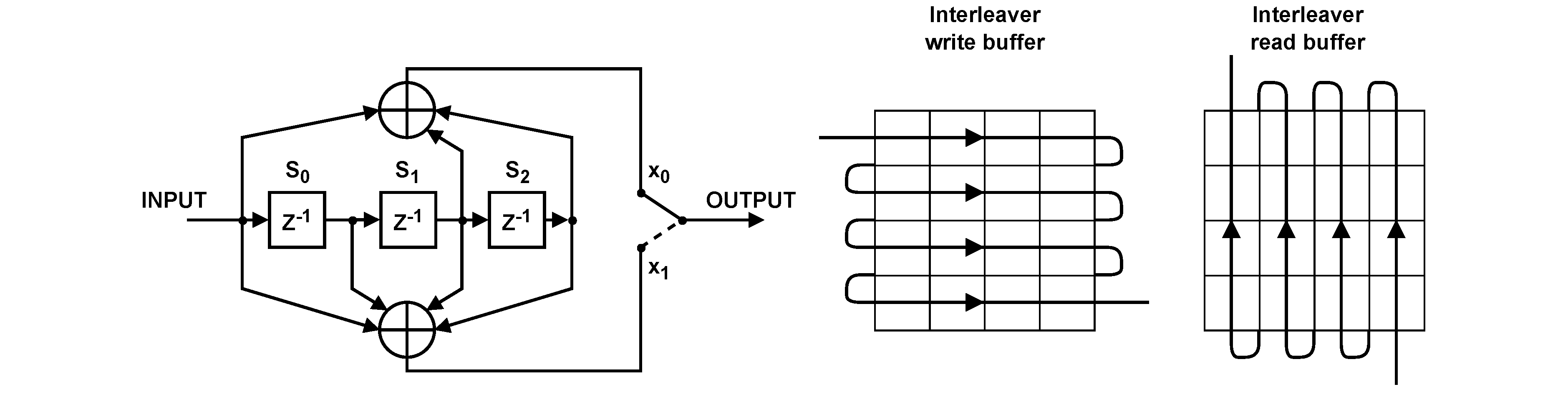
The first stage includes a 1/2 rate non-recursive convolutional encoding process with a constraint length (L) of 4. The 1/2 base coding rate indicates that each input bit will be encoded into two output bits. The encoder itself consists of three shift registers where an XOR operation is applied twice in a specific manner, eventually gaining two output bits.
The second stage applies a 32-bit interleaving process executed on every 2-bit symbols. This interleave/deinterleave process scrambles and separates adjacent symbols, thus lowering the impact of bursty errors that mostly span multiple bits and can be induced by interference or time-varying signal strengths. In this way, the process increases the robustness against these errors [31]. In order to have a properly working interleaving process, a convolutional code trellis terminator is also appended to the unencoded data. This sequence is 0x0B0B for even-length byte input and 0x0B0B0B for odd-length byte input. In the DASH7 protocol, a 4x4 matrix interleaver is used.
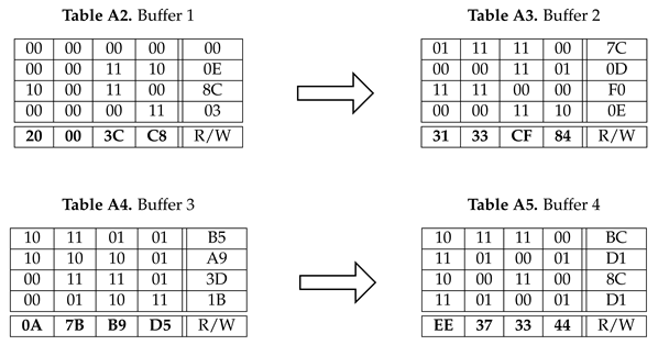
The bits coming from the convolutional coder are written into the rows of the matrix interleaver while the bits that will be sent are read from the columns of the matrix in a certain order. The interleaving operation is applied per 2-bit symbols. This means that the data is scrambled per 32 aligned bits. Note that FEC is only applied when using Coding Scheme 2 of DASH7 where the data firstly is FEC encoded and afterwards PN9 encoded. Figure A1 depicts the operation of the encoder stage and interleaving stage. The following example is based on [32] whereas Table A4 shows the filled buffers of the interleaver. The output bytes are highlighted in bold.
Example
| Input [4 B] | 0x03 | 0x01 | 0x02 | 0x03 | ||||
| Appended CRC [6 B] | 0x03 | 0x01 | 0x02 | 0x03 | 0x7E | 0x2D | ||
| Appended Trellis terminator [8 B] | 0x03 | 0x01 | 0x02 | 0x03 | 0x7E | 0x2D | 0x0B | 0x0B |
| FEC encoder output [16 B] | 00 | 0E | 8C | 03 | 7C | 0D | F0 | 0E | B5 | A9 | 3D | 1B | BC | D1 | 8C | D1 |
| Interleaver output [16 B] | C8 | 3C | 00 | 20 | 84 | CF | 33 | 31 | D5 | B9 | 7B | 0A | 44 | 33 | 37 | EE |
Figure A1.
Implementation of the FEC operation in DASH7 starting with a convolutional encoder with configuration (n,k,m) = (2,1,3) where n is the number of output bits, k is the number of input bits and m is the number of shift register stages supplemented with the 4x4 matrix interleaver.
Figure A1.
Implementation of the FEC operation in DASH7 starting with a convolutional encoder with configuration (n,k,m) = (2,1,3) where n is the number of output bits, k is the number of input bits and m is the number of shift register stages supplemented with the 4x4 matrix interleaver.
Appendix C. PN9 Coding
The 9-bit pseudo-random number (“PN9”) generator is shown at the top of Figure A2. The generator is described by the polynomial . The PN9 generates all the values between 1 through 511 (inclusively) in a pseudo-random order as it is clocked. The latches are all set to ones at the start of a whitening operation.
Figure A2.
PN9 Coding Circuit.
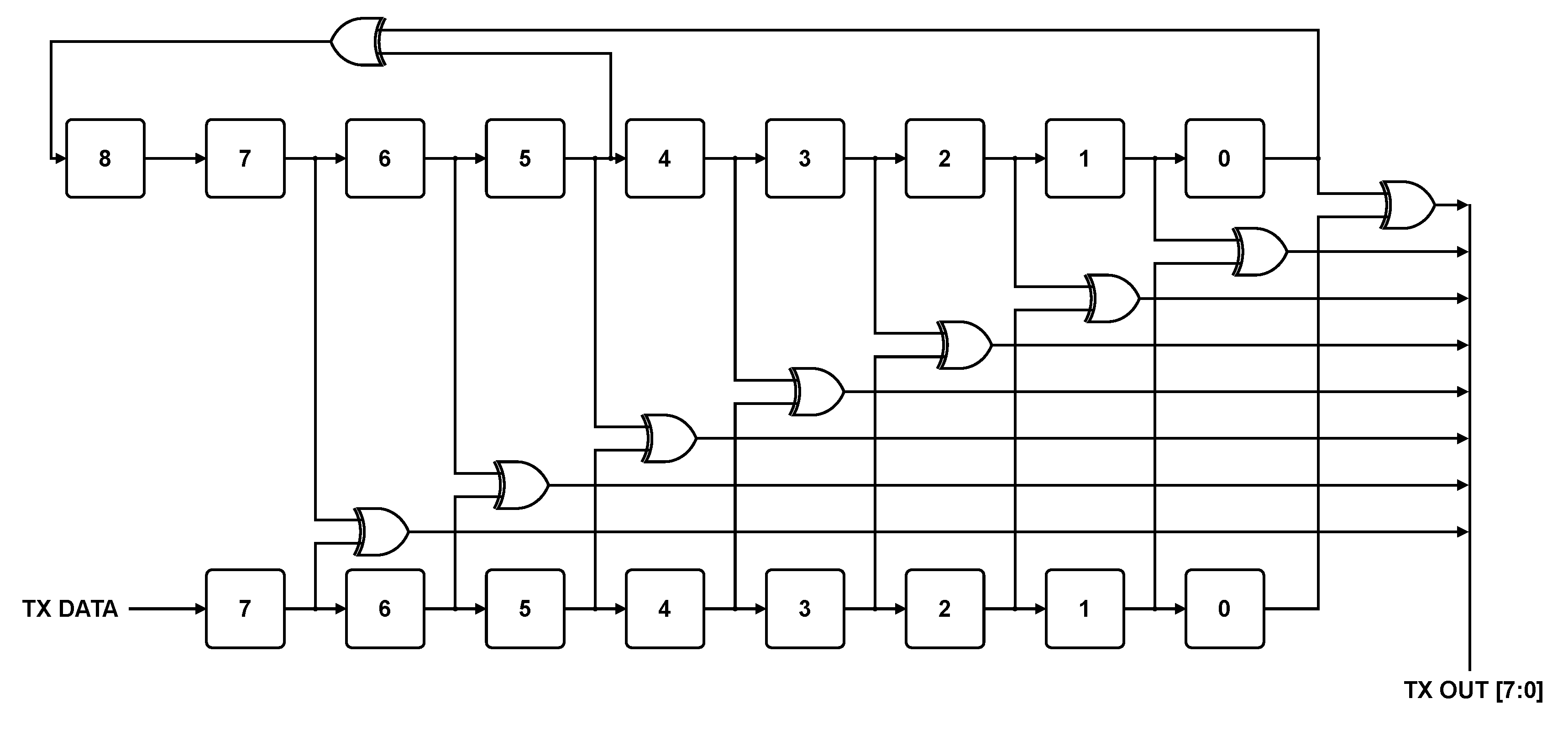
Figure A3.
Operation of the PN9 generator.
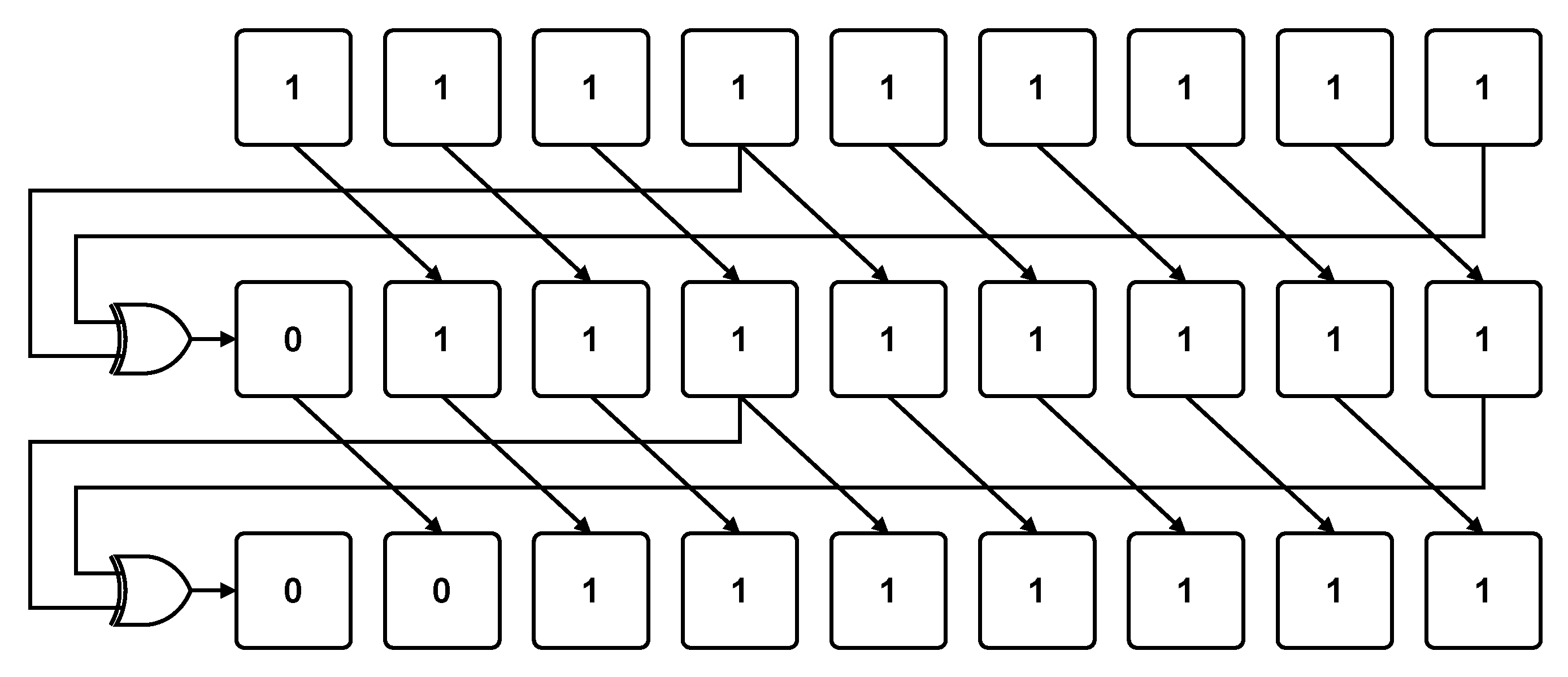
Figure A3 illustrates the operation of the PN9 generator as it is clocked. The generator starts with a value of all ones “111111111”. Bit 0 (the LSB) and bit 5 are XOR’d to produce 0 that is shifted into the MSB on the next clock. This results in the next value of the generator being “011111111”. Again, bits 0 and 5 are XOR’d to give the next value of the MSB (again, 0) to produce the next value of the generator “001111111”, and the process continues through all 511 states of the generator.
Whitening Operation The lower set of latches in Figure A2 contains the current byte of the data to be whitened. Recall that the preamble and sync words are not whitened, so the first byte of data to be whitened is either the packet length byte (in variable packet mode) or the first byte of user data.
When the first byte of data is ready, it is XOR’d with the eight LSBs of the initial value of the PN9 generator, which are all ones. So, the PN9 generator is “111111111”, and the data is XOR’d with the eight LSBs of this, which is “11111111”. This whitened data is then transmitted over the air. Next, the second byte of data is shifted into the data latches (eight shifts, one per bit), while the PN9 generator is also clocked eight times (once per bit). This means that the second byte of user data is not XOR’d with the next PN9 value but instead by the value eight later in the PN9 sequence. Thus, the PN9 generator contains “111111111” when the first byte is processed, while the PN9 generator state during the second byte of data is not “011111111” (the next PN9 value), but instead “111100001” (the ninth PN9 value).
Example
Suppose the (unwhitened) data sequence to be transmitted starts out as (these would be the bytes, for example, if a packet with a packet length byte of ten were transmitted, and the data was 0x00, 0x01,... ): / 0000 1010 / 0000 0000 / 0000 0001 / 0000 0010 / ..., Remember that the values to XOR with the data are the eight LSBs of the PN9 sequence if every eighth value is used:
1,1,1,1,1,1,1,1,1 *** Eight LSBs are 1111 1111
0,1,1,1,1,1,1,1,1
0,0,1,1,1,1,1,1,1
0,0,0,1,1,1,1,1,1
0,0,0,0,1,1,1,1,1
1,0,0,0,0,1,1,1,1
1,1,0,0,0,0,1,1,1
1,1,1,0,0,0,0,1,1
1,1,1,1,0,0,0,0,1 *** Eight LSBs are 1110 0001
0,1,1,1,1,0,0,0,0
1,0,1,1,1,1,0,0,0
1,1,0,1,1,1,1,0,0
1,1,1,0,1,1,1,1,0
0,1,1,1,0,1,1,1,1
0,0,1,1,1,0,1,1,1
0,0,0,1,1,1,0,1,1
0,0,0,0,1,1,1,0,1 *** Eight LSBs are 0001 1101
1,0,0,0,0,1,1,1,0
0,1,0,0,0,0,1,1,1
1,0,1,0,0,0,0,1,1
1,1,0,1,0,0,0,0,1
0,1,1,0,1,0,0,0,0
0,0,1,1,0,1,0,0,0
1,0,0,1,1,0,1,0,0
1,1,0,0,1,1,0,1,0 *** Eight LSBs are 10011010
0,1,1,0,0,1,1,0,1
So, the values to XOR with the data are:
/ 1111 1111 / 1110 0001 / 0001 1101 / 1001 1010/
Taking the exclusive-OR of these two sequences gives the data to be transmitted:
Data: / 0000 1010 / 0000 0000 / 0000 0001 / 0000 0010 ...
PN9: / 1111 1111 / 1110 0001 / 0001 1101 / 1001 1010/ ...
Result: / 1111 0101 / 1110 0001 / 0001 1100 / 1001 1000 /...
When received, the resultant data is XOR’d with the same PN9-derived sequence, resulting into the originally transmitted data. Received: / 1111 0101 / 1110 0001 / 0001 1100 / 1001 1000 /...
PN9: / 1111 1111 / 1110 0001 / 0001 1101 / 1001 1010/ ...
Data: / 0000 1010 / 0000 0000 / 0000 0001 / 0000 0010 / ...
References
- Zanella, A.; Bui, N.; Castellani, A.; Vangelista, L.; Zorzi, M. Internet of Things for Smart Cities. IEEE Internet of Things journal 2014, 1, 22–32.
- Centenaro, M.; Vangelista, L.; Zanella, A.; Zorzi, M. Long-range Communications in Unlicensed Bands: The Rising Stars in the IoT and Smart City Scenarios. IEEE Wireless Communications 2016, 23, 60–67.
- Bni Lam, N.H. Angle of arrival estimation for low power and long range communication networks. PhD thesis, University of Antwerp, 2021.
- BniLam, N.; Janssens, R.; Steckel, J.; Weyn, M. AoA estimates for LPWAN technologies: Indoor experimental analysis. 2021 15th European Conference on Antennas and Propagation (EuCAP). IEEE, 2021, pp. 1–5.
- BniLam, N.; Steckel, J.; Weyn, M. Synchronization of multiple independent subarray antennas: An application for angle of arrival estimation. IEEE Transactions on Antennas and Propagation 2019, 67, 1223–1232.
- BniLam, N.; Joosens, D.; Steckel, J.; Weyn, M. Low Cost AoA Unit for IoT Applications. 2019 13th European Conference on Antennas and Propagation (EuCAP), 2019, pp. 1–5.
- BniLam, N.; Ergeerts, G.; Subotic, D.; Steckel, J.; Weyn, M. Adaptive probabilistic model using angle of arrival estimation for IoT indoor localization. 2017 International Conference on Indoor Positioning and Indoor Navigation (IPIN), 2017, pp. 1–7.
- DASH7 Alliance. http://www.dash7-alliance.org, accessed on 10.09.2024.
- Sub-IoT. https://sub-iot.github.io/Sub-IoT-Stack, accessed on 10.09.2024.
- Mekki, K.; Bajic, E.; Chaxel, F.; Meyer, F. A Comparative Study of LPWAN Technologies for Large-scale IoT Deployment. ICT express 2019, 5, 1–7.
- Semtech. https://www.semtech.com, accessed on 10.09.2024.
- Janssen, T.; BniLam, N.; Aernouts, M.; Berkvens, R.; Weyn, M. LoRa 2.4 GHz communication link and range. Sensors 2020, 20, 4366.
- BniLam, N.; Nasser, S.; Weyn, M. Angle of Arrival Estimation System for LoRa Technology based on Phase Detectors. 2022 16th European Conference on Antennas and Propagation (EuCAP), 2022, pp. 1–5.
- Adefemi Alimi, K.O.; Ouahada, K.; Abu-Mahfouz, A.M.; Rimer, S. A Survey on the Security of Low Power Wide Area Networks: Threats, Challenges, and Potential Solutions. Sensors 2020, 20, 5800.
- BniLam, N.; Joosens, D.; Aernouts, M.; Steckel, J.; Weyn, M. LoRay: AoA estimation system for long range communication networks. IEEE Transactions on Wireless Communications 2020, 20, 2005–2018.
- Wang, Y.P.E.; Lin, X.; Adhikary, A.; Grovlen, A.; Sui, Y.; Blankenship, Y.; Bergman, J.; Razaghi, H.S. A Primer on 3GPP Narrowband Internet of Things. IEEE communications magazine 2017, 55, 117–123.
- Bembe, M.; Abu-Mahfouz, A.; Masonta, M.; Ngqondi, T. A Survey on Low Power Wide Area Networks for IoT Applications. Telecommunication Systems 2019, 71, 249–274.
- Bnilam, N.; Joosens, D.; Berkvens, R.; Steckel, J.; Weyn, M. AoA-based localization system using a single IoT gateway: An application for smart pedestrian crossing. IEEE Access 2021, 9, 13532–13541.
- Price, N.D.; Zawodniok, M.J.; Guardiola, I.G. Transceivers as a Resource: Scheduling Time and Bandwidth in Software-Defined Radio. IEEE Access 2020, 8, 132603–132613.
- GNU Radio. https://www.gnuradio.org/, accessed on 10.09.2024.
- DASH7 Alliance. DASH7 Alliance Protocol Specification v1.2. https://www.dash7-alliance.org/download-specification/, accessed on 10.09.2024.
- Norair, J. Introduction to DASH7 Technologies, 1st ed., 2009.
- Singh, R.K.; Puluckul, P.P.; Berkvens, R.; Weyn, M. Energy Consumption Analysis of LPWAN Technologies and Lifetime Estimation for IoT Application. Sensors 2020, 20, 4794.
- Sklar, B. Digital Communications: Fundamentals & Applications, Second Edition; Prentice Hall, 2001.
- Lyons, R. Understanding Digital Signal Processing; Prentice Hall, 2011.
- Proakis, J.; Salehi, M. Digital Communications 5th Edition; McGraw Hill, 2007.
- Mueller, K.; Muller, M. Timing recovery in digital synchronous data receivers. IEEE transactions on communications 1976, 24, 516–531.
- Joosens, D.; BniLam, N.; Weyn, M.; Berkvens, R. SDR-based IoT Communication Systems: An Application for the DASH7 Alliance Protocol. Data set on Zenodo 2024. [CrossRef]
- Joosens, D.; BniLam, N.; Weyn, M.; Berkvens, R. Implementation of a Multi-Channel DASH7 IoT Communication System for Packet Investigation and Validation, 2024. [CrossRef]
- Semtech. SX1276/77/78/79 - 137 MHz to 1020 MHz Low Power Long Range Transceiver. https://semtech.my.salesforce.com/sfc/p/#E0000000JelG/a/2R0000001Rbr/6EfVZUorrpoKFfvaF_Fkpgp5kzjiNyiAbqcpqh9qSjE, accessed on 10.09.2024.
- Weyn, M.; Ergeerts, G.; Wante, L.; Vercauteren, C.; Hellinckx, P. Survey of the DASH7 alliance protocol for 433 MHz wireless sensor communication. International Journal of Distributed Sensor Networks 2013, 9, 870430.
- Hoel, R. Design Note DN504 FEC implementation. Texas Instruments, 2007. Rev. 2.
| 1 |
Product-to-sum identities:
|
| 2 | In our presentation, the symbols take the values of [-1,1] and are converted directly from the binary data [0,1]. However, the samples represent the digital waveform that will be transmitted. Therefore, the sample rate will always be larger than the symbol rate. |
Figure 1.
Functional block diagram of a direct conversion or zero-IF based SDR architecture. Note that the parallel lines indicate that this process is repeated,i.e., one flow is dedicated to the In-phase data stream and one flow to the Quadrature data stream.
Figure 1.
Functional block diagram of a direct conversion or zero-IF based SDR architecture. Note that the parallel lines indicate that this process is repeated,i.e., one flow is dedicated to the In-phase data stream and one flow to the Quadrature data stream.
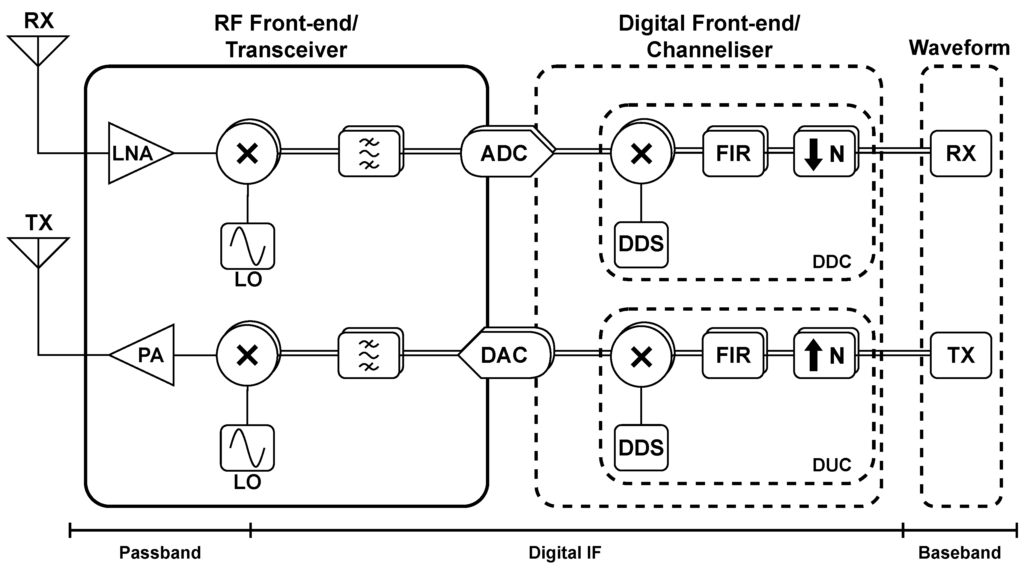
Figure 3.
Two-dimensional spectrogram of ten modulated DASH7 packets seen over 1.4 seconds and a bandwidth of 200 kHz.
Figure 3.
Two-dimensional spectrogram of ten modulated DASH7 packets seen over 1.4 seconds and a bandwidth of 200 kHz.
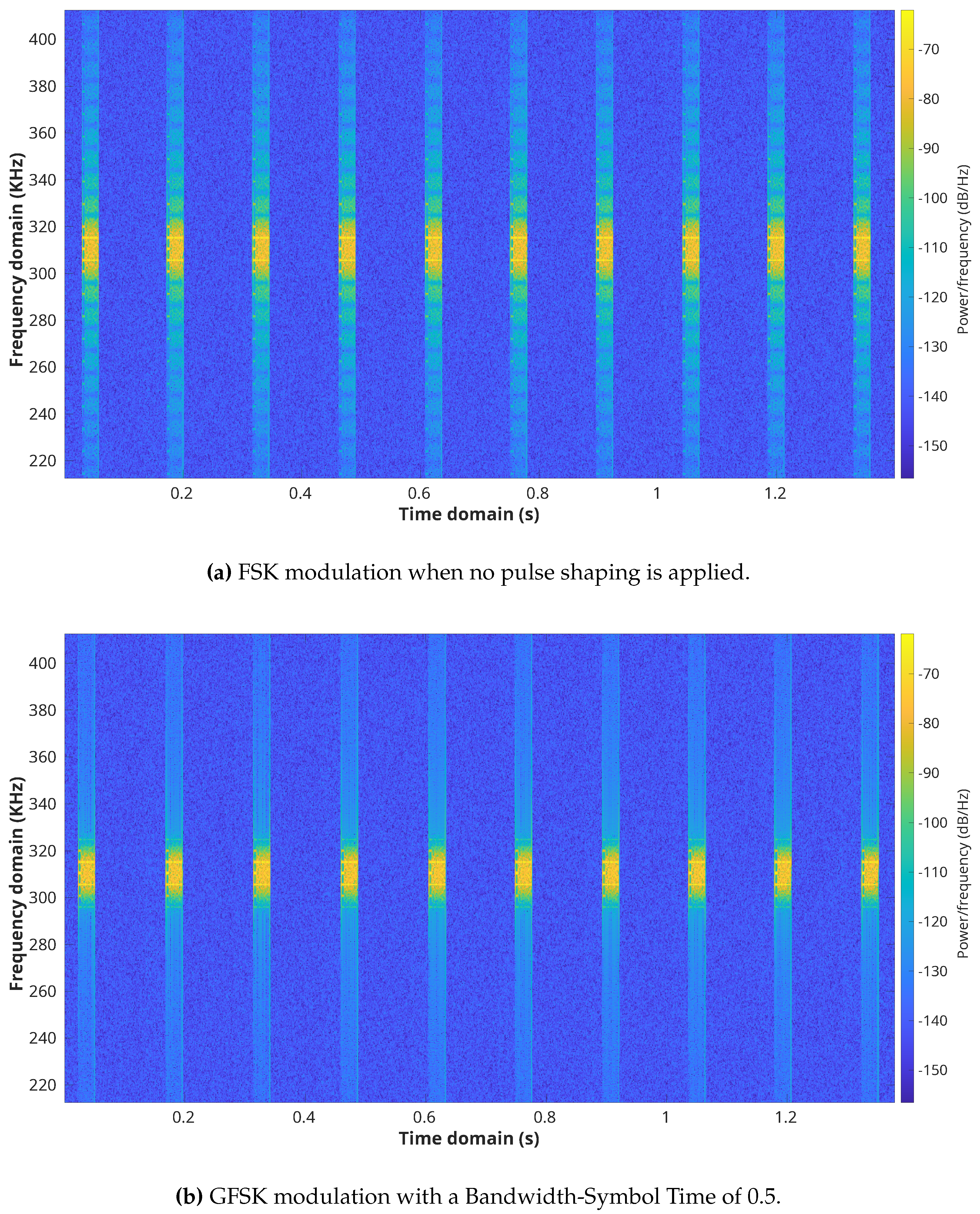
Figure 4.
Three-dimensional spectrogram of ten modulated DASH7 packets seen over 1.4 seconds and a bandwidth of 200 kHz.
Figure 4.
Three-dimensional spectrogram of ten modulated DASH7 packets seen over 1.4 seconds and a bandwidth of 200 kHz.
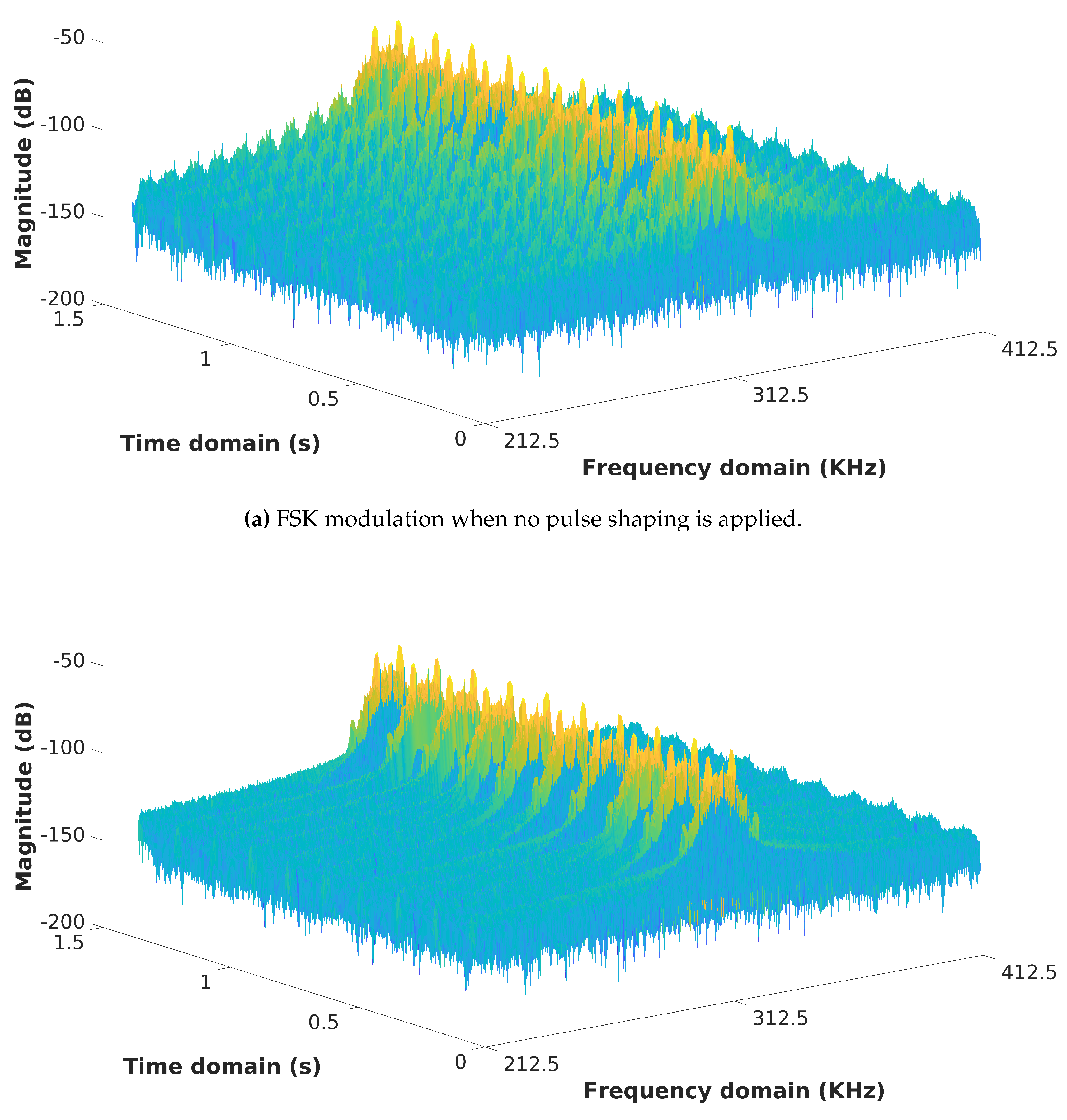
Figure 5.
DASH7 packet structure.

Figure 6.
Packet to symbols conversion. The data formatting box exploits three vector sources and a multiplexer block. The values of the vector sources are controlled by the respective parameters. The second blue framed box converts the byte’s parallel values into a series of symbols where the 0b is represented by -1 and the 1b is represented by 1. The complete transmitted packet is presented in Figure 7.
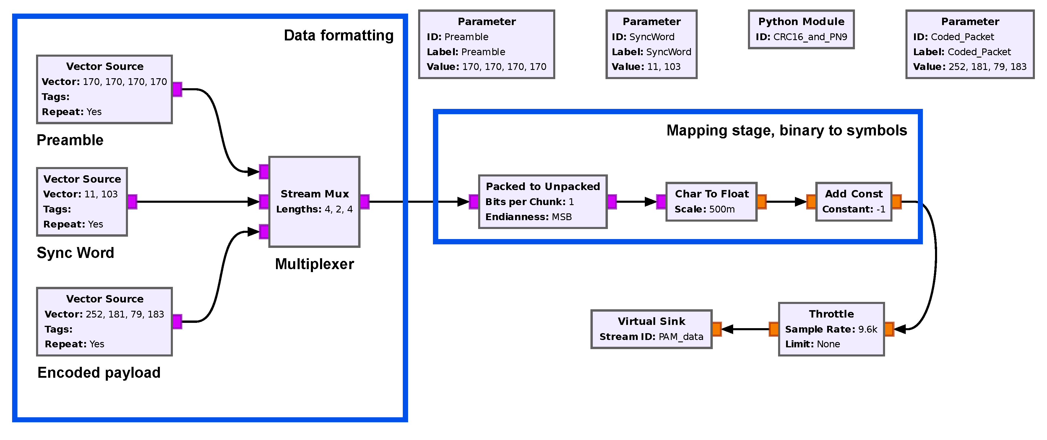
Figure 7.
DASH7 mapped packet structure. The figure shows the preamble followed by the sync word and the whitened payload in the time domain.
Figure 7.
DASH7 mapped packet structure. The figure shows the preamble followed by the sync word and the whitened payload in the time domain.
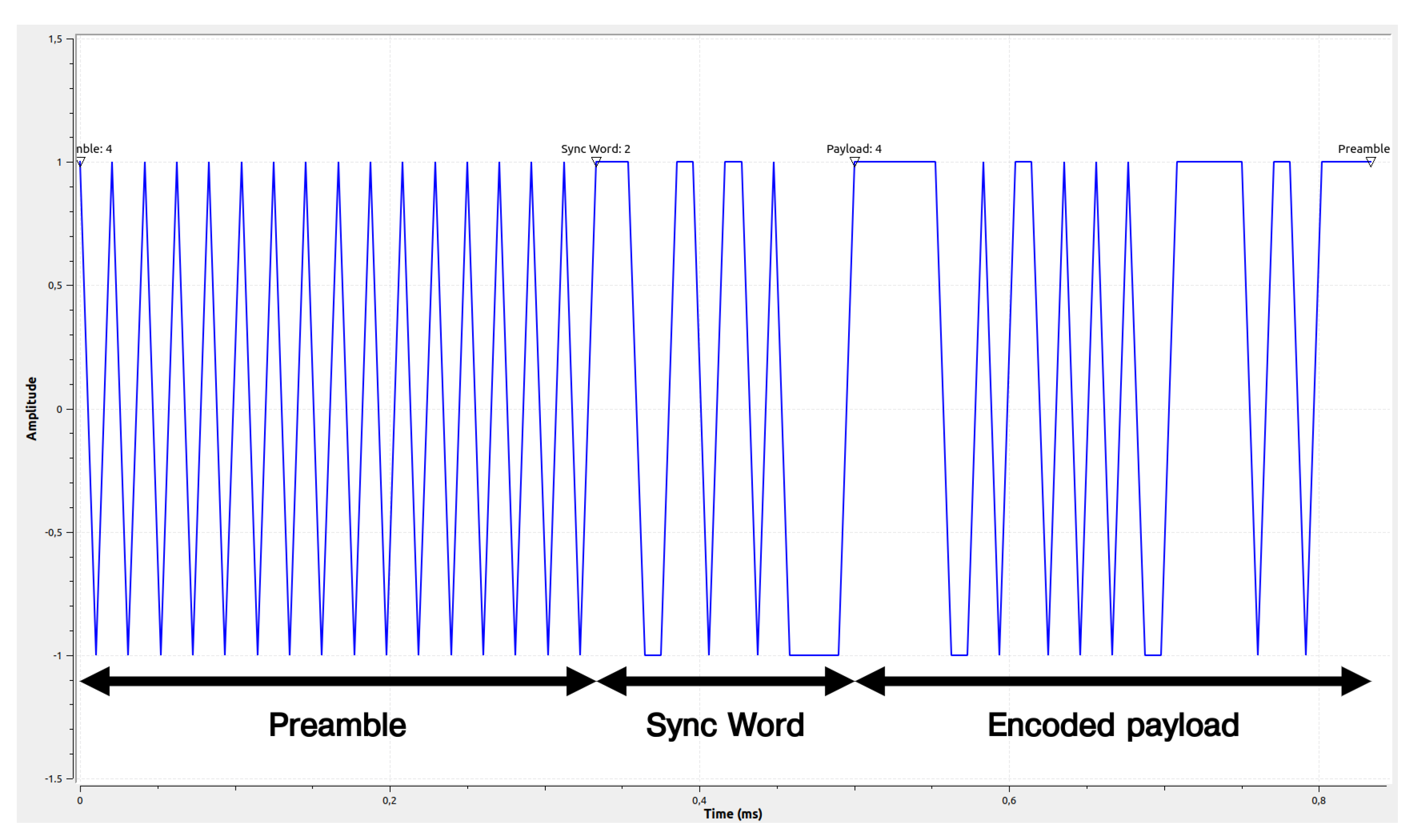
Figure 8.
The upsampling process and shape filter process in GNU Radio, which is achieved with an interpolating FIR filtering.
Figure 8.
The upsampling process and shape filter process in GNU Radio, which is achieved with an interpolating FIR filtering.
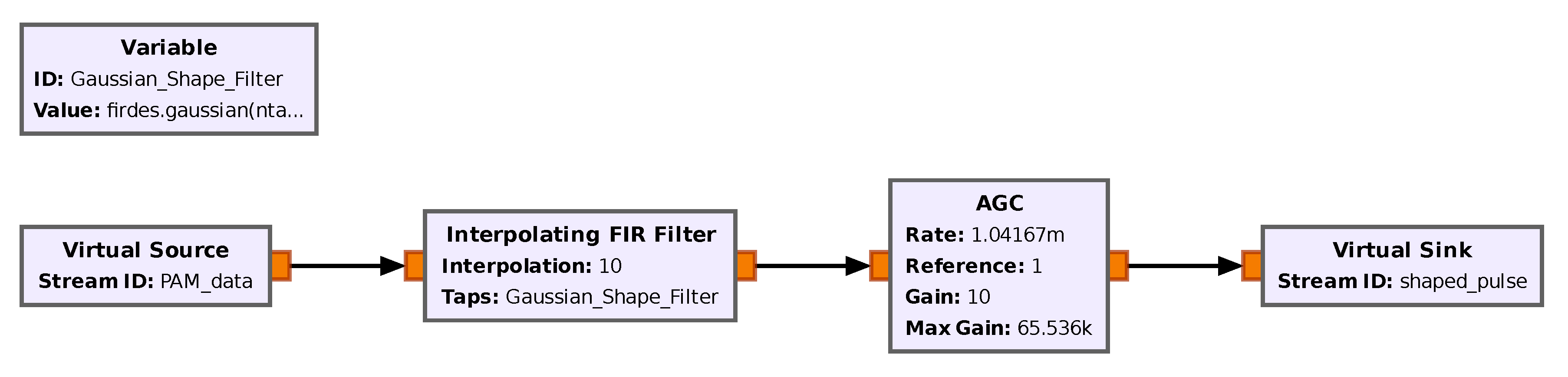
Figure 9.
The generated waveform as seen in the time domain.
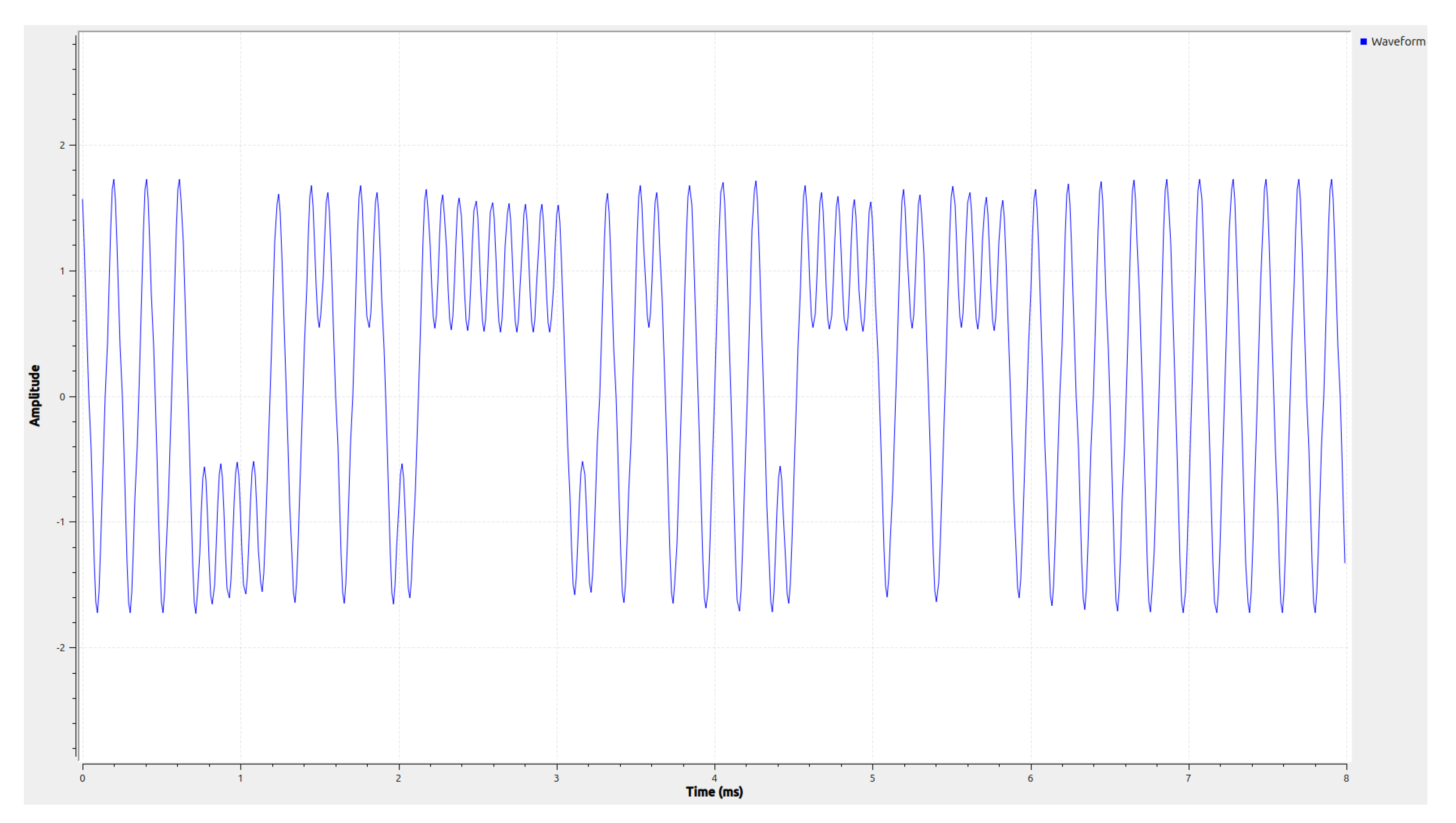
Figure 10.
Flowgraph of the GFSK modulation. The FSK modulation constitutes majorly of an IIR filter with configurable taps that act as an integrator and a phase to complex value block.
Figure 10.
Flowgraph of the GFSK modulation. The FSK modulation constitutes majorly of an IIR filter with configurable taps that act as an integrator and a phase to complex value block.
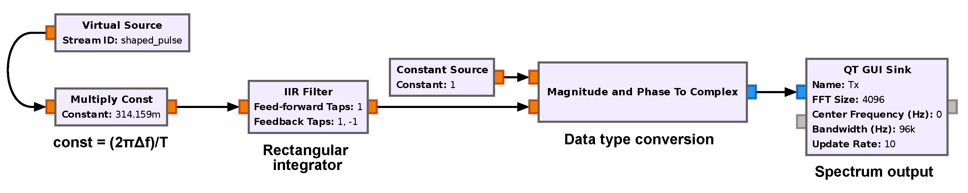
Figure 11.
Frequency response of a baseband modulated DASH7 signal.
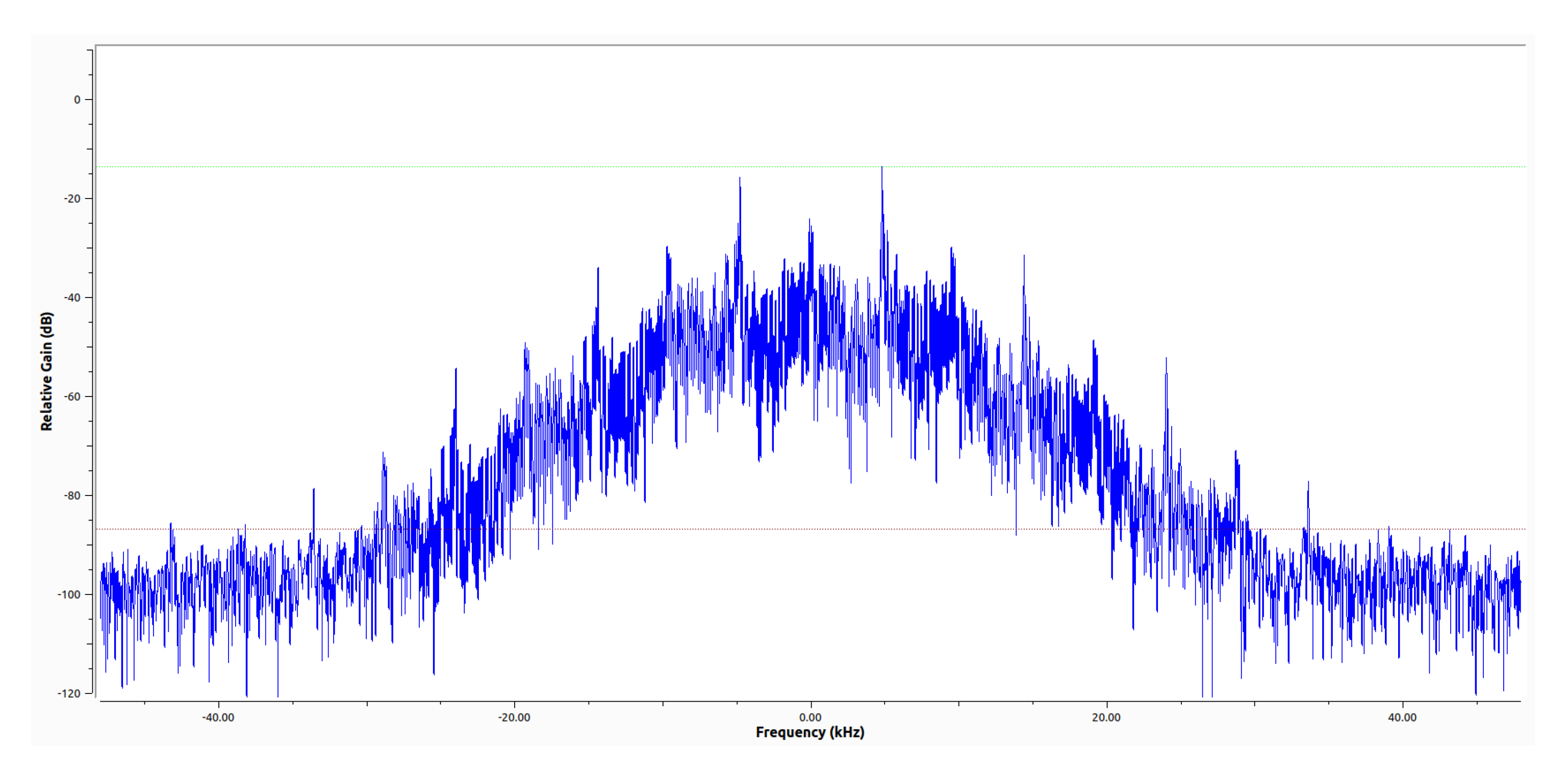
Figure 12.
Fixed frequency demodulator using recorded data while tuned to channel 0 using the Lo-Rate channel class.
Figure 12.
Fixed frequency demodulator using recorded data while tuned to channel 0 using the Lo-Rate channel class.
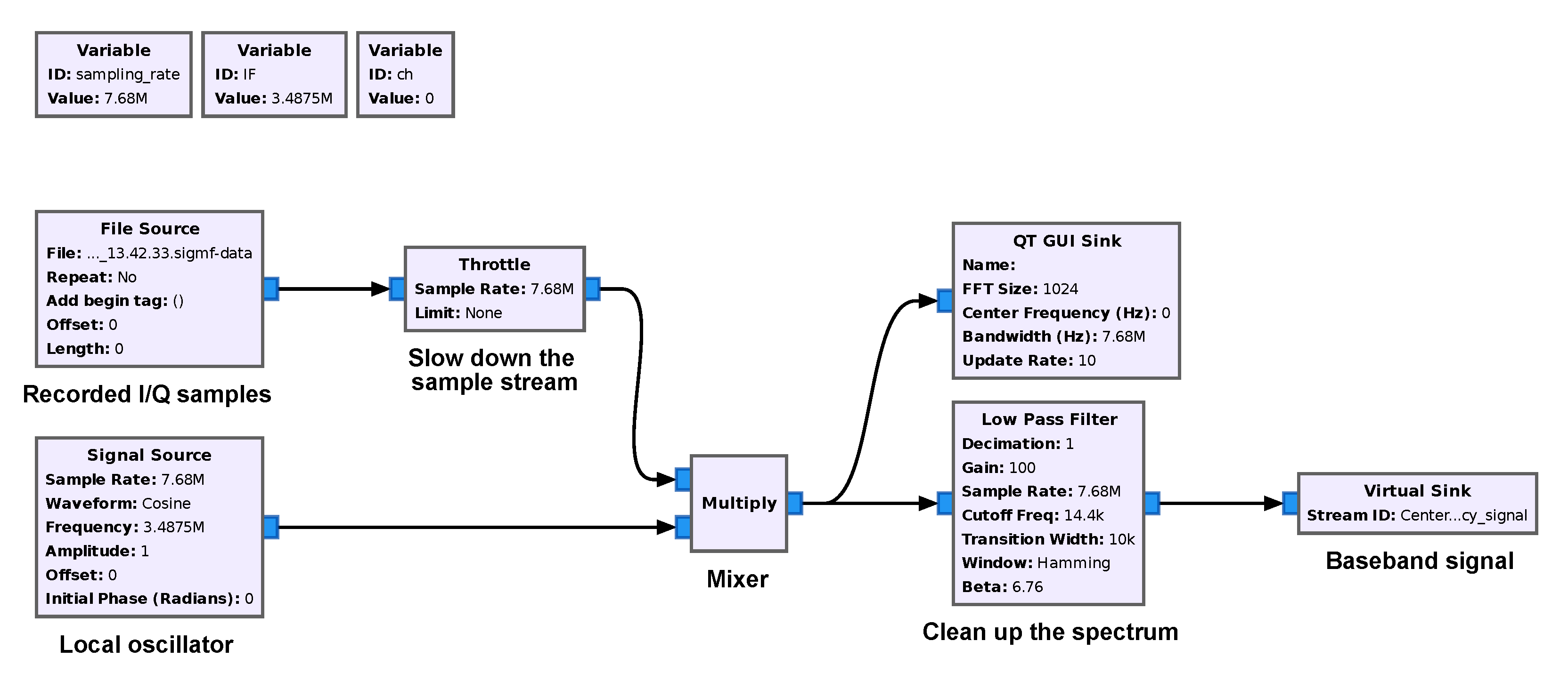
Figure 13.
Demodulation process. The phase is extracted from the data signal and consecutively accumulated, and high-frequency noise is filtered out.
Figure 13.
Demodulation process. The phase is extracted from the data signal and consecutively accumulated, and high-frequency noise is filtered out.
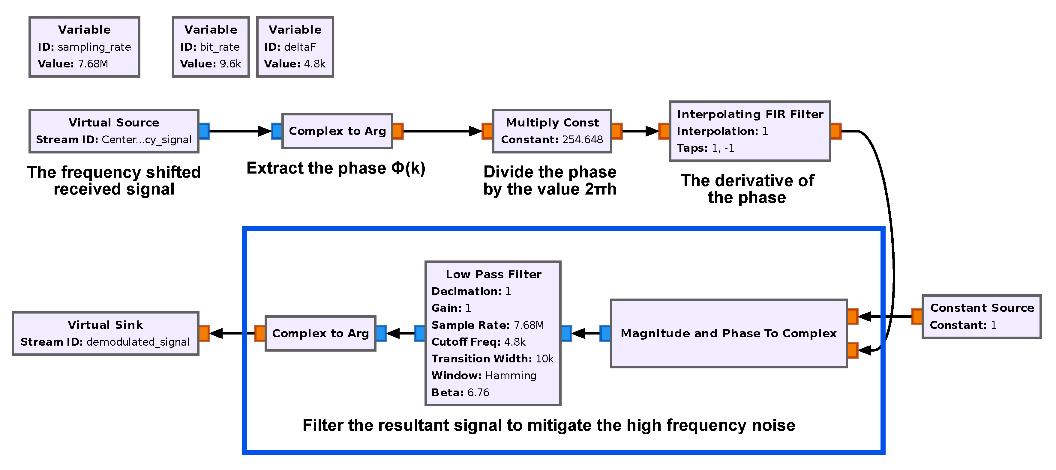
Figure 15.
Decoded output of a DASH7 packet with a length of 25 bytes as seen in the console window of GNU Radio. The packet has a payload of three bytes [0x00, 0xAB, 0xCD] followed by two CRC bytes.
Figure 15.
Decoded output of a DASH7 packet with a length of 25 bytes as seen in the console window of GNU Radio. The packet has a payload of three bytes [0x00, 0xAB, 0xCD] followed by two CRC bytes.
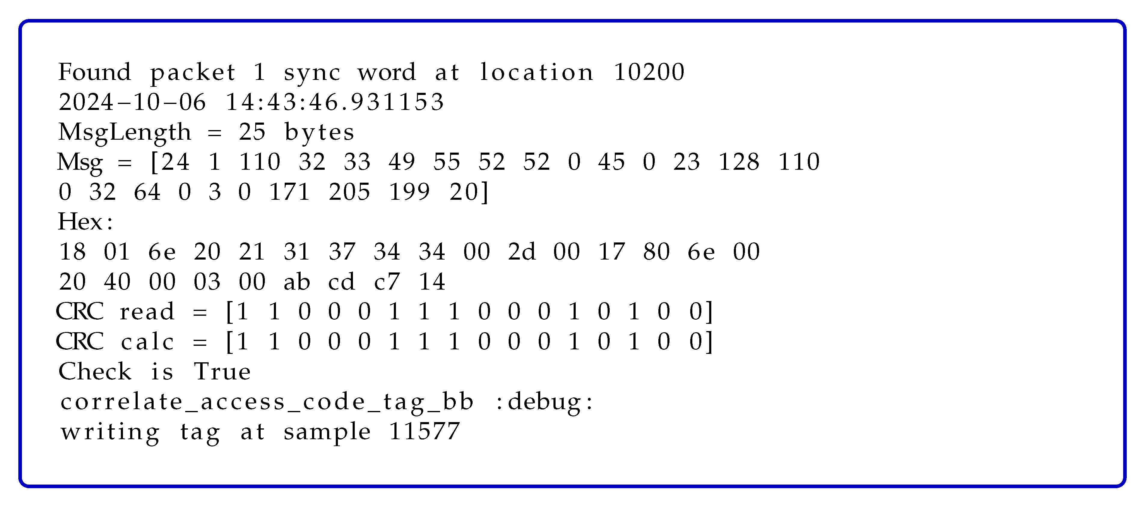
Figure 16.
Measurement setup with three DASH7 nodes and three DASH7 gateways which send and receive on different Lo-Rate channels. The setup is extended with an Ettus Research USRP B210 SDR, which records the transmissions of the DASH7 nodes and stores them as raw I/Q data, which are investigated during post-processing analysis.
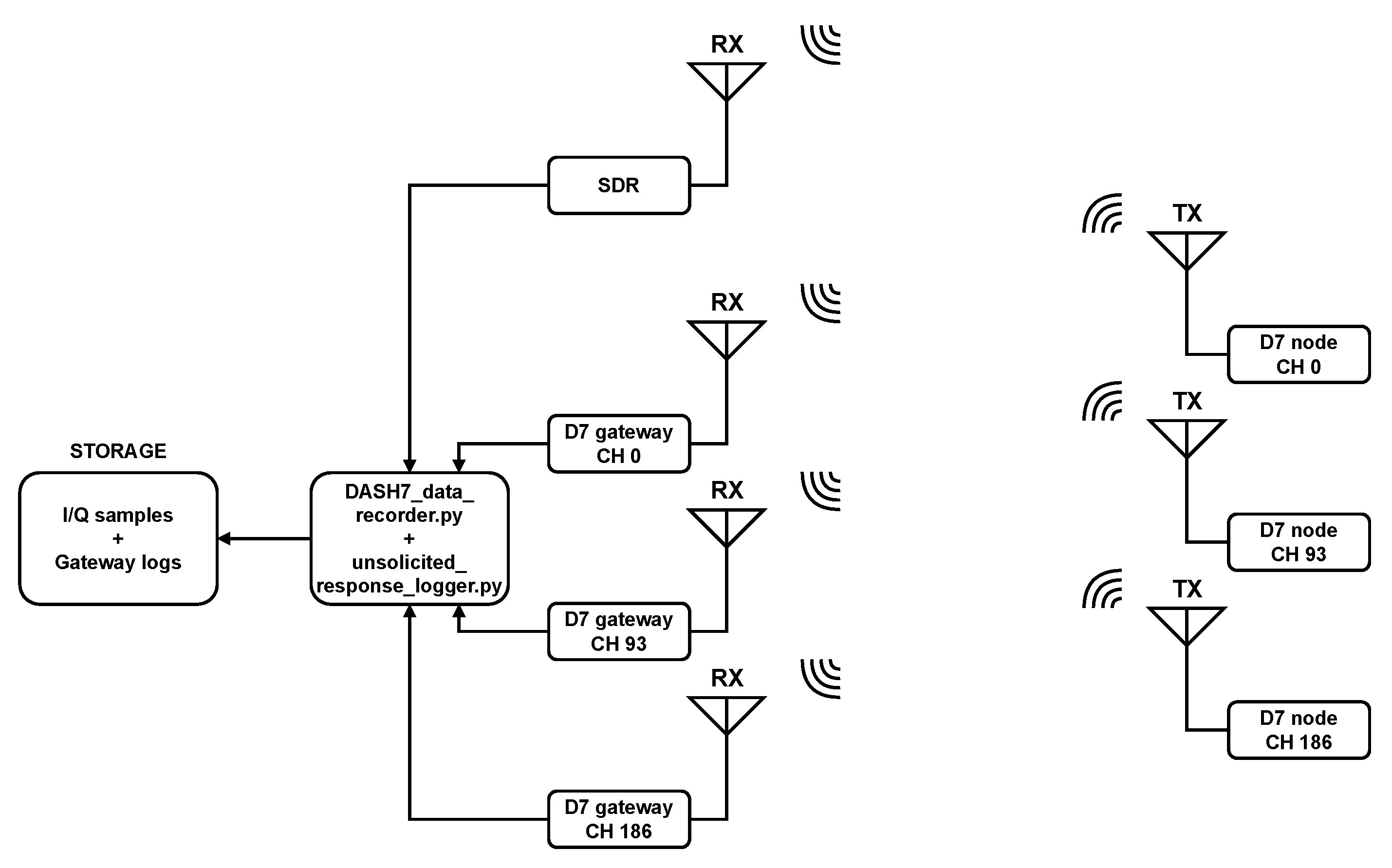
Figure 17.
The cabled measurement setup consisting of a DASH7 gateway a DASH7 node and Software Defined Radio.
Figure 17.
The cabled measurement setup consisting of a DASH7 gateway a DASH7 node and Software Defined Radio.
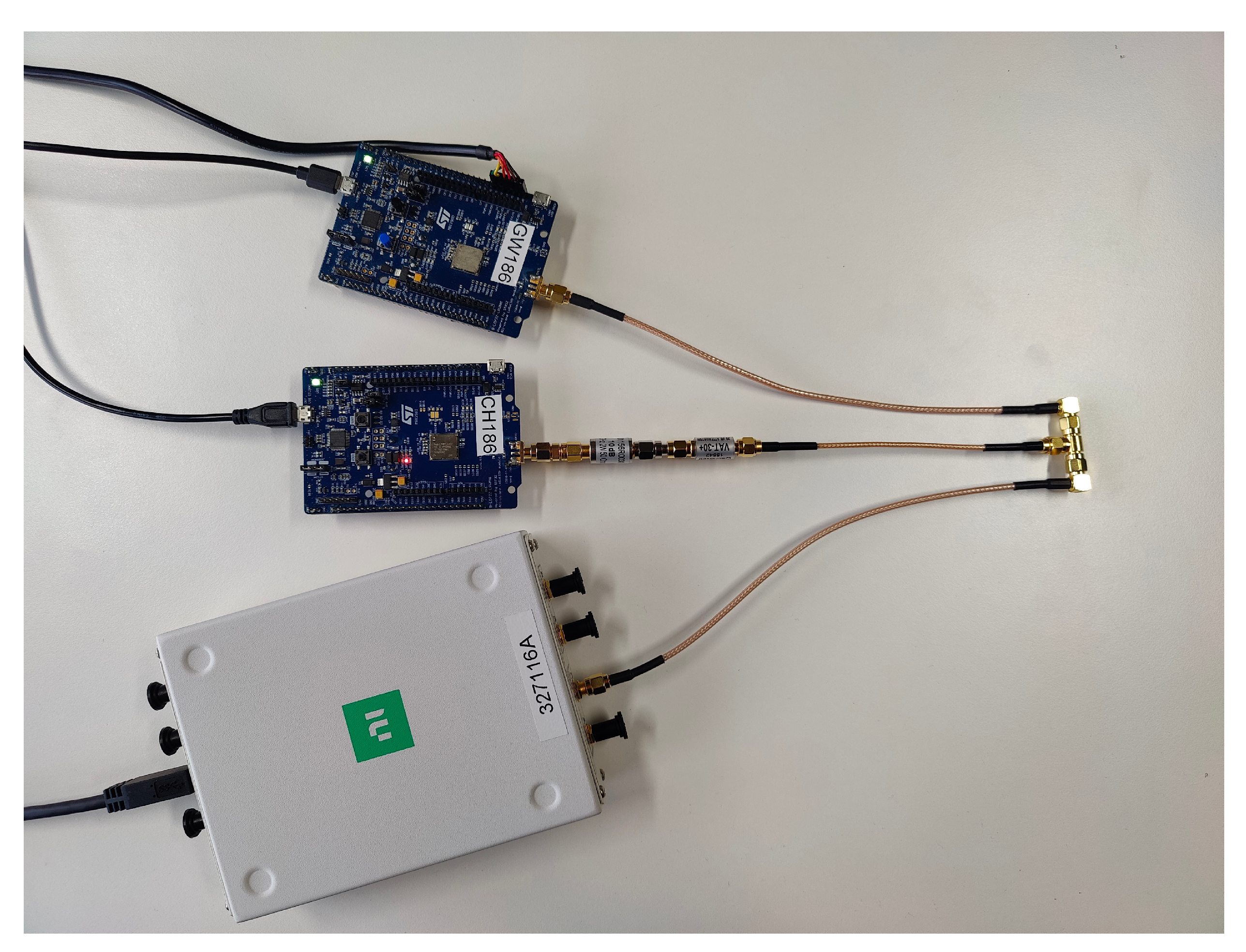
Figure 18.
Map of the indoor measurement environment. The 10 TX locations are shown as green pins while the receiving setup, i.e. the SDR and DASH7 gateways are positioned at the red RX pin.
Figure 18.
Map of the indoor measurement environment. The 10 TX locations are shown as green pins while the receiving setup, i.e. the SDR and DASH7 gateways are positioned at the red RX pin.
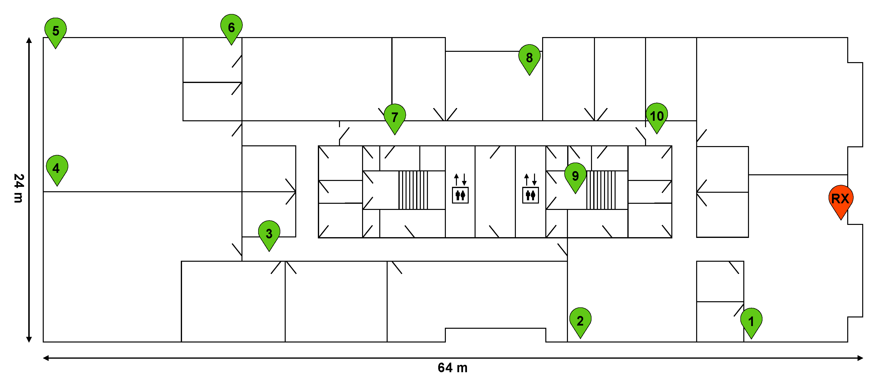
Figure 19.
Map of the suburban measurement environment.
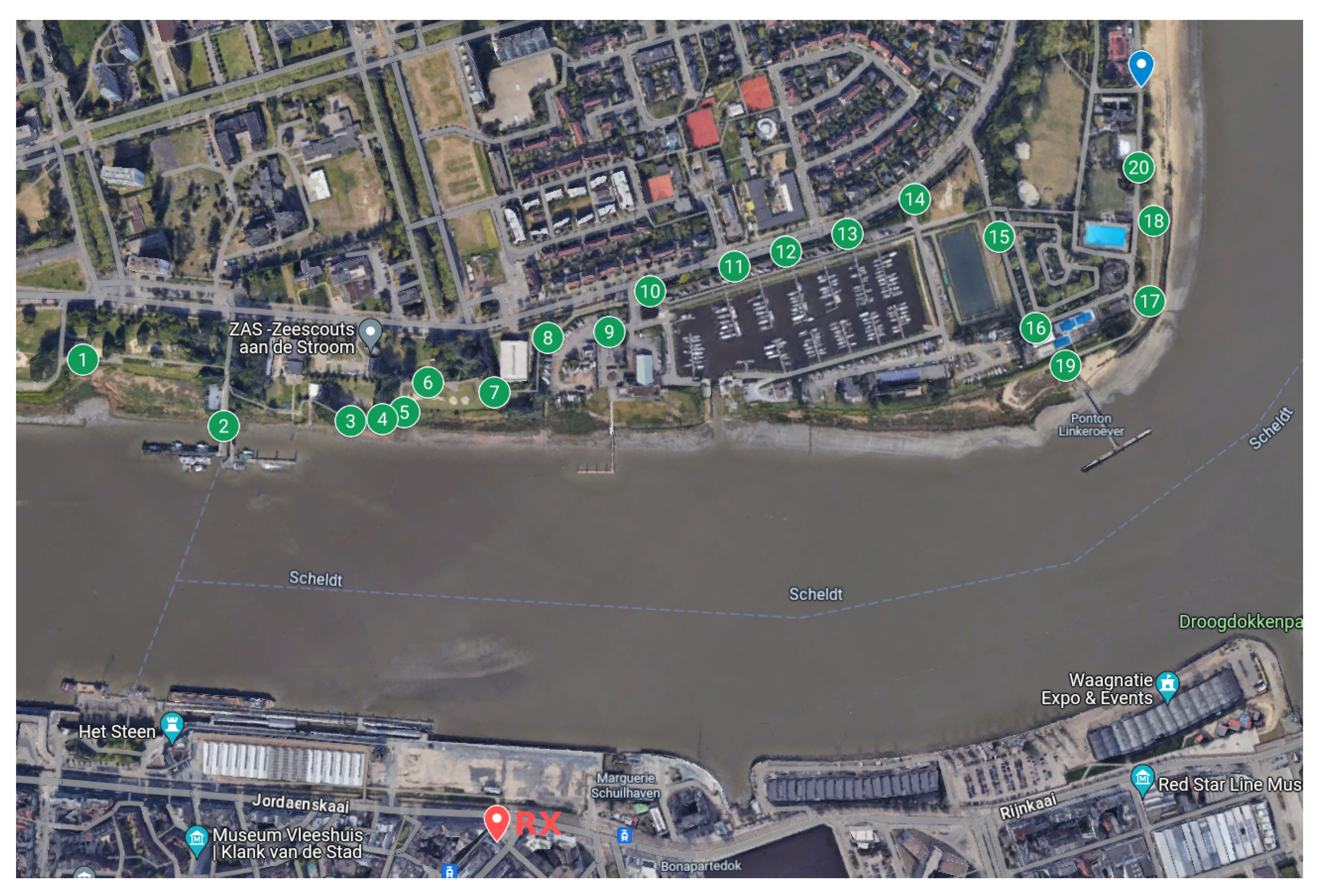
Table 2.
Non-exhaustive list of common SDRs that can be used for the reception of LPWAN protocols.
| SDR | Frequency (MHz) |
ADC/DAC resolution |
Max. RF bandwidth |
RF channels |
Price |
|---|---|---|---|---|---|
| RTL-SDR Blog V3 | 24 - 1766 | 8-bit | 3.2 MHz | 1 RX | $ |
| Great Scott Gadgets | 1 - 6000 | 8-bit | 20 MHz | 1 TX/RX | $$ |
| HackRF one | |||||
| Analog Devices | 325 - 3800 | 12-bit | 20 MHz | 1 TX - 1 RX | $$ |
| ADALM-PLUTO | |||||
| Nuand | 70 - 6000 | 12-bit | 56 MHz | 2 TX - 2 RX | $$ |
| bladeRF 2.0 xA4 | |||||
| Ettus Research | 70 - 6000 | 12-bit | 56 MHz | 1 TX - 1 RX | $$ |
| USRP B200mini | |||||
| Ettus Research | 70 - 6000 | 12-bit | 56 MHz | 1 TX - 1 RX | $$ |
| USRP B200 | |||||
| Ettus Research | 70 - 6000 | 12-bit | 56 MHz | 2 TX - 2 RX | $$$ |
| USRP B210 | |||||
| Deepwave Digital | 300 - 6000 | 14-16 bit | 100 MHz | 2 TX - 2 RX | $$$$ |
| AIR7201-B |
Table 3.
DASH7 channel bands. The stars in the table indicate the following: * Worldwide coverage with local regulatory limitations, ** EN 300 220 (Europe) with local regulatory limitations, *** FCC part 15 in the United States of America.
Table 3.
DASH7 channel bands. The stars in the table indicate the following: * Worldwide coverage with local regulatory limitations, ** EN 300 220 (Europe) with local regulatory limitations, *** FCC part 15 in the United States of America.
| RF band | Lo-Rate (d) | Normal and Hi-Rate (d) | Start (b) | End |
|---|---|---|---|---|
| 433 MHz* | 0, 1, ..., 68 | 0, 8, 16, ..., 56 | 433.06 MHz | 434.785 MHz |
| 868 MHz** | 0, 1, ...., 279 | 0, 8, 16, ..., 216, 229, 239, 257, 270 | 863 MHz | 870 MHz |
| 915 MHz*** | 0, 1, ..., 1039 | 0, 8, 16, ..., 1032 | 902 MHz | 928 MHz |
Table 4.
DASH7 channel classes.
| Class | Symbol Rate | Modulation Index | Frequency Deviation | Channel Spacing (c) |
|---|---|---|---|---|
| Lo-Rate | 9.6 kbps | 1 | ± 4.8 kHz | 0.025 MHz |
| Normal | 55.555 kbps | 1.8 | ± 50 kHz | 0.2 MHz |
| Hi-Rate | 166.667 kbps | 0.5 | ± 41.667 kHz | 0.2 MHz |
Table 5.
DASH7 sync word classes. Currently, only CS0 and CS2 are used. CS1 and CS3 are reserved for future use.
Table 5.
DASH7 sync word classes. Currently, only CS0 and CS2 are used. CS1 and CS3 are reserved for future use.
| Sync Word Class | Coding Scheme | |||
|---|---|---|---|---|
| CS0 | CS1 | CS2 | CS3 | |
| 0 | 0xE6D0 | RFU | 0xF498 | RFU |
| 1 | 0x0B67 | RFU | 0x192F | RFU |
Table 6.
Comparison of the packet loss found at each DASH7 gateway and packet loss in software per location for three Lo-Rate channels for the outdoor experiment. Furthermore, the logged mean received signal strengths at each DASH7 gateway and the gateway-to-node distance are shown.
Table 6.
Comparison of the packet loss found at each DASH7 gateway and packet loss in software per location for three Lo-Rate channels for the outdoor experiment. Furthermore, the logged mean received signal strengths at each DASH7 gateway and the gateway-to-node distance are shown.
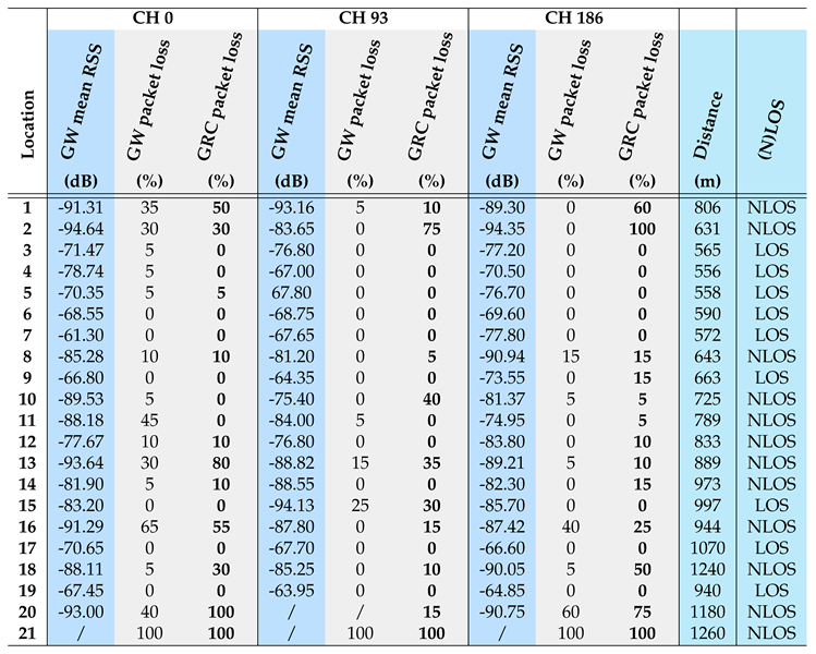
Table 7.
Mean received signal strength and packet loss per location for three Lo-Rate channels for the indoor experiment.
Table 7.
Mean received signal strength and packet loss per location for three Lo-Rate channels for the indoor experiment.
Disclaimer/Publisher’s Note: The statements, opinions and data contained in all publications are solely those of the individual author(s) and contributor(s) and not of MDPI and/or the editor(s). MDPI and/or the editor(s) disclaim responsibility for any injury to people or property resulting from any ideas, methods, instructions or products referred to in the content. |
© 2024 by the authors. Licensee MDPI, Basel, Switzerland. This article is an open access article distributed under the terms and conditions of the Creative Commons Attribution (CC BY) license (http://creativecommons.org/licenses/by/4.0/).
Copyright: This open access article is published under a Creative Commons CC BY 4.0 license, which permit the free download, distribution, and reuse, provided that the author and preprint are cited in any reuse.


