Submitted:
02 July 2024
Posted:
03 July 2024
You are already at the latest version
Abstract
Aiming at the problems of inaccurate segmentation of long object and information loss of small object in real-time semantic segmentation algorithm, this paper proposes a lightweight multi-branch real-time semantic segmentation network based on BiseNetV2. The new auxiliary branch makes full use of spatial details and context information to cover the long object in the field of view. Meanwhile, in order to ensure the inference speed of the model, the asymmetric convolution is used in each stage of the auxiliary branch to design a structure with low computational complexity. In the multi-branch fusion stage, the alignment and fusion module is designed to provide guidance information for deep and shallow feature mapping, so as to make up for the problem of feature misalignment in the fusion of information at different scales, and thus reduce the loss of small target information. In order to further improve the model’s awareness of key information, a global context module is designed to capture the most important features in the input data. The proposed network uses NVIDIA GeForce RTX 3080 Laptop GPU experiment, on the road street view data set Cityscapes and CamVid average occurring simultaneously ratio reached 77.1% and 78.4% respectively, with running speed of 127 frames/s respectively and 112 frames/s. The experimental results show that the proposed algorithm can achieve real-time segmentation and improve the accuracy significantly, showing good semantic segmentation performance
Keywords:
Semantic segmentation
; Asymmetric convolution
; Feature misalignment
; High-level semantic information
1. Introduction
Image semantic segmentation is an important research content in the field of computer vision. By classifying and predicting a given image pixel by pixel, this method can segment different areas of semantic identification, which has a wide range of applications in many fields such as automatic driving, scene analysis, medical detection and machine perception [1,2,3,4,5].
In recent years, with the rapid development of artificial intelligence, deep learning technology has been widely applied in the field of image semantic segmentation and has achieved better results than traditional image segmentation algorithms [6,7,8,9,10,11]. Since the convolution network (Fully Convolutional Networks, FCN) [12] connects traditional convolution neural networks in the whole layer is replaced by convolution, based on the depth of the convolution of the neural network approach [13] has become the main solution of semantic segmentation task. It has brought a new research direction for other image semantic segmentation researchers, and prompted many high-precision image semantic segmentation algorithms to be proposed. Among them, in order to refine the spatial details, PSPNet [14] designed a Pyramid Pooling Module (PPM, a new paper published in Acta Electronica) and used global average pooling operations to extract global information. In order to reduce the problem of spatial information loss during downsampling, DeepLab [15,16,17,18,19] uses void convolution to increase the receptive field to obtain more context information. On this basis, the emerging optimized and improved version of Deep Lab algorithm [20] has gradually improved the accuracy of semantic segmentation. In order to extract features with different resolutions, HRNet [21] realizes image semantic segmentation with high accuracy by maintaining high image resolution and conducting parallel subsampling.
The above semantic segmentation networks perform well in segmentation accuracy, but this high accuracy mainly depends on their complex model design, which usually requires a large number of parameters and computational resources, and is difficult to meet the needs of real-time processing, thus limiting their practical application. Therefore, real-time semantic segmentation algorithms with fewer parameters and faster running speed have become a research focus [22,23,24,25,26]. Early real-time semantic segmentation networks often used efficient encoder-decoder structures [27,28,29]. ICNet [30] uses a cascading network structure to gradually encode features of different resolutions, effectively improving the model running speed. FANet [31] uses a bidirectional feature pyramid network to fuse feature information at different levels in the decoder stage. These methods have made progress in real-time, but the reduction of a large number of model parameters will weaken the ability of network structure to extract feature information. Therefore, some research methods design a special module for extracting features to improve the segmentation performance of the model. ESPNet [32] designed the Efficient Spatial Pyramid (ESP) module, which improved the accuracy of the network while reducing the number of parameters and calculation cost of the network model. SwiftNet [33] adopts a structure with Spatial Pyramid Pooling (SPP) in the downsampling phase to reduce the amount of model calculation. EADNet [34] design multi-scale shape feeling more wild convolution (Multi-scale Multi-shape Receptive Field Convolution, MMRFC) module, and use the module built a lightweight semantic network segmentation. The inference speed of the above network is greatly improved, but the model sacrifices the spatial resolution in order to realize the real-time inference speed, resulting in the loss of the feature spatial information.
For this reason, BiSeNet [35] chose a lightweight backbone network and proposed an additional downsampling path to obtain spatial details and integrate it with the backbone network to compensate for the reduced accuracy. On this basis, BiSeNetV2 [36] improved the structure of BiSeNet by reducing the number of channels, adopting fast downsampling strategy, and introducing auxiliary training strategy to further improve segmentation performance.
This two-branch network achieves a better balance in terms of inference speed and segmentation accuracy. However, the detailed branch network structure of BiseNetV2 is shallow, which causes the extracted features to lack sufficient receptive field. At the same time, the symmetric convolution adopted by this branch will capture interference information from irrelevant regions [37], which will not effectively identify target objects that may be long (such as grass) or dispersed (such as traffic signs) structures, and ultimately lead to lower segmentation accuracy. In addition, the way BiseNetV2 fuses multi-branch features has the problem of feature misalignment [38], thus ignoring the diversity between the two branches, which is not conducive to recovering the feature information lost by small targets during network downsampling.
Finally, since the semantic branch of BiseNetV2 in the network is to capture global context information and extract high-level semantic features, it needs to be further improved to enhance the model’s ability to extract high-level semantic features. To solve the above problems, this paper optimizes BiseNetV2 to improve the performance of the algorithm. The main contributions of this paper are summarized as follows: (1) Auxiliary branches are designed to guide detailed branches to capture long distance relationships between features, further increasing the segmentation performance of large irregular targets. (2) the proposed alignment and integration module (Alignment And Fusion Module AAFM) to merge multiple output branch of the model in the implementation of effective interaction between multiple branch at the same time ease characteristics not alignment problem, so as to make up for the loss of small target information. (3) A Global Context Mudule (CGM) module is introduced to capture the most important features in the input data, thereby improving the model’s awareness of key information.(4) The performance of the proposed algorithm on Cityscapes and CamVid data sets is significantly improved compared with BiseNetV2 algorithm and other existing advanced algorithms, which proves the superiority of the proposed algorithm.
2. Textual Algorithm
2.1. Overall Structure
The network structure of the BiseNetV2 algorithm and the proposed algorithm is shown in Figure 1. Figure 1(a) is the BiseNetV2 algorithm, and Figure 1(b) is the improved proposed algorithm based on BiseNetV2.
As shown in Figure 1(a), BiseNetV2 uses detail branches and semantic branches respectively to obtain spatial detail information and semantic abstract information.
In this paper, the BiseNetV2 algorithm is optimized and improved. As shown in Figure 1(b), the network is designed into three branches, among which the detail branch and auxiliary branch are responsible for extracting spatial detail features, and the semantic branch is responsible for capturing semantic context features. Finally, the features of the three branches are fused to obtain semantic segmentation results. The overall structure of the multi-branch network algorithm proposed in this paper is shown in Figure 2. The backbone network consists of three branches, namely the detail branch (blue branch), the auxiliary branch (yellow branch), and the semantic branch (green branch). The numbers in each branch box represent the ratio of the feature map size to the resolution of the original input. First, the image is extracted by three branches in parallel. The auxiliary branches are fused with the detail branches at each stage to help the model better retain spatial information. When the feature of the semantic branch is extracted to 1/32 of the original feature, the global context module is embedded to further enhance the context representation ability. In addition, the Alignment and fusion module is used when features are fused. The module feeds the features obtained from the detail branch through downsampling (Down) and the features obtained from the semantic branch through the Sigmoid activation function () into the alignment layer (AL). At the same time, the features obtained by the semantic branch after upsampling (Up) and Sigmoid activation function () and the features obtained by the detail branch are also sent to the alignment layer, so that the features of the two branches are fully aligned and interactive fusion. Finally, the two outputs from the alignment layer are added (SUM) to the output of the secondary branch. In addition, this algorithm retains the auxiliary training strategy of the baseline model, and promotes the feature extraction capability of different shallow networks by combining the loss of four auxiliary heads and the loss of the main network segment head. The three modules proposed in this paper are described in detail: auxiliary branch, alignment and fusion module, and global context module.
2.2. Auxiliary Branch
BiSeNetV2 uses symmetric convolution to form detail branches to extract low-level features from images. However, the disadvantages of symmetric convolution are obvious: (1) Symmetric convolution considers all directions equally and may ignore valid texture information; (2) They have a fixed kernel size and are not suitable for processing input data with different shapes or aspect ratios, which leads to limited processing capacity for diverse input data; (3) Due to its inherent symmetry and inherent smoothing effect, it may lead to the loss of details and texture information in some cases. In order to solve the above problems, this algorithm proposes a new auxiliary branch structure to capture information such as long-range dependencies, edges, textures, etc. The new auxiliary branch structure is shown in Figure 3.
The new auxiliary branch consists of three stages, as shown in Figure 3(a), where the red box represents the convolution process. The first stage of the branch uses convolution with step 2 to extract high-resolution features from the input features; In the second stage, convolution with step size 1 is used to increase the receptive field and capture the long range relationship of isolated regions, so as to achieve segmentation of large targets. In the third stage, the convolution operation with step size 1 is further used to encode and integrate the detailed features extracted before. For the first stage, input X is obtained by vertical asymmetric convolution, and then it is sent to horizontal asymmetric convolution to obtain. The operations in the latter two stages of the auxiliary branch are similar to this stage. The operation process of each stage is shown as follows:
where, is the input of this branch, represents an asymmetric convolution operation with a convolution kernel size of m×n, and and are the features obtained after vertical and horizontal asymmetric convolution, respectively. The process of auxiliary branching is shown in Figure 3(b). In the first stage of the detail branch, the image resolution is high and there is sufficient detail information. In order to avoid model redundancy, this algorithm does not assist this stage. Instead, it fuses the feature FD1 of the first stage of the detail branch with the feature of the first stage of the auxiliary branch to get , then uses to guide the second stage of the detail branch to get , and then fuses it with the output of the second stage of the auxiliary branch to get . And use it to guide the third phase of the detail branch. In this way, auxiliary branch feature and detail branch feature are gradually integrated to realize the interaction of feature information at different scales, further establish the dependency relationship between discrete distribution regions, and enhance edge and texture information, thus providing a more comprehensive and rich feature representation. The specific operation process is shown as follows:
where, , and represent auxiliary branches, detail branches and their integrated feature maps respectively, . represents the broadcast operation, and represents the convolution operation, where "⊕" represents the element-by-element addition operation.
In addition, for real-time semantic segmentation models, besides performance, the model speed should be considered. The reasons for choosing asymmetric convolution to form new auxiliary branches will be explained from the point of view of velocity. Consider that the baseline model is a convolution layer with dimension and space dimension . Without loss of generality, suppose , decomposed into two convolution layers of size and , respectively. The computational cost of these two schemes is directly proportional to and respectively. Therefore, a significant improvement can be obtained when . The analysis of the above formula shows that the new auxiliary branch does not bring too much computational burden.
2.3. Align and Fuse Modules
BiseNetV2 proposes a bidirectional guided aggregation module to fuse and guide the detail branches and semantic branches. Although effective communication is achieved through mutual guidance between the two branches, it does not take into account the misalignment of features that may occur when the two branches are merged. This will lead to the two branches passing invalid information to each other, and produce feature redundancy after fusion, which is not conducive to deep feature recovery of small target details. To solve this problem, a new alignment and fusion module is designed to fuse the three branches of the network. The structure is shown in Figure 4. This module is introduced in two parts: the first part guides the detail branches for the semantic branches; The second part guides the semantic branch for the detail branch.
Detail branches guide semantic branches: The guidance stage is shown in FIG. Figure 4(a) in orange. First, detail branch features are obtained by 3×3 convolution to obtain local features, and then channel dimensionality is reduced by average pooling operation. Meanwhile, semantic branching features undergo 3×3 deep separable convolution to increase their receptive fields, followed by 1×1 convolution to integrate features. Finally, they are fused to by element multiplication to achieve efficient guidance between the two branches. In the alignment stage, as shown in Figure 4(a), the gray part is shown. Firstly, the is learned through 3×3 convolution prediction to obtain the two-dimensional offset , in which each pixel position contains the horizontal and vertical offset. According to the two-dimensional offset , the relative position relationship between pixels with different resolution features can be obtained. Then, the semantic branch feature is Warp by using two-dimensional offset to get . Warp is a kind of spatial transformation operation. As shown in Figure 4(b), a spatial grid is generated through the offset, which is used to resampleth the image, thereby generating the aligned feature map and alleviating the problem of feature misalignment in the fusion of feature maps with different resolutions.
Semantic branches guide detailed branches: Similar to the above operation, the two branches guide each other to get , which is then sent to the 3×3 convolution operation for convolution, learning and predicting the two-dimensional offset . Then, Warp with to get . Finally, and are connected according to channel dimension.
Finally, in the purple part of FIG. Figure 4(a), in order to avoid the redundant features in the fusion diagram, a 3×3 convolution operation is used to obtain . In addition, when the final three branches are fused, in order to save parameters, the algorithm combines and by adding pixels of corresponding positions to get the final output F. The above operation process is shown as follows:
where, represents the input of this module, represents detail branch, semantic branch and auxiliary branch respectively; represents the convolution operation m×n; Apooling indicates average pooling operation. The Warp operation is shown in Figure 4b. ⊗ represents the multiplication-by-element operation.
2.4. Global Context Module
In order to give full play to the key role of high-level semantic information in semantic branches, a global context module is designed to retain image information more effectively. Traditional methods often use stacked convolutional layers to extract high-level semantic features, but this approach consumes a lot of computing resources. In order to realize real-time performance, the algorithm adopts global average pooling and global maximum pooling in the global context module instead of stacking convolution layers. Among them, global average pooling is not limited by the size of receptive field and operates on the entire feature map, so it can capture a wider range of contextual information, which helps the model understand the semantics and structure of the overall image, and provides global visual perception. By selecting the maximum activation value within each channel, the most significant features can be extracted, which helps to focus attention on the most important features in the image, thus enhancing the perception and differentiation ability of the model for key information.
The module structure is shown in Figure 5. Firstly, the input feature of this module is globally average pooled and globally maximum pooled respectively, and then the two obtained feature maps are batch normalized to stabilize the distribution of input features. Then, in order to extract more effective features, 1×1 convolution is used to process them separately to fuse features from different channels and realize the interaction between different channel features. Then, the expression ability of the model was enhanced by batch normalization and ReLU activation function, and and were obtained. , , and are then fused using skip connections to directly pass information about input features to and , helping to strike a balance between processing details and global information. Finally, in order to better represent the semantic information in the image, 3×3 convolution is carried out to further enhance the abstraction ability and get the output . The above operations can be expressed as follows:
and represent the input and output of the module respectively. GAP and GMP represent global average pooling and global maximum pooling, respectively. represents a convolution operation with a convolution kernel size of m×n; and represent ReLU and BatchNorm operations, respectively.
3. Experiment and Result Analysis
3.1. Data Set Introduction
3.1.1. Cityscapes Data Set
The Cityscapes dataset [39] consists of 25,000 high-resolution street view images from 50 different cities in Germany. The resolution of the images in the dataset is 1024×2048, consisting of 5000 finely annotated and 2000 roughly annotated images. The algorithm is trained and validated using finely labeled images, which are grouped into 19 categories comprising a training dataset (2,975 images), a validation dataset (500 images), and a test dataset (1,525 images). Similar to the advanced semantic segmentation methods [15,36], 19 common semantic categories (such as sidewalk, road, and car) are used in this experiment.
3.1.2. CamVid Data Set
CamVid [40]is a computer vision dataset widely used in semantic segmentation tasks, mainly for image segmentation and semantic annotation in urban scenes. The dataset, which includes video images captured by cameras while cars are driving, covers a variety of scenes and objects such as city streets, traffic signs, pedestrians, and vehicles, and has lower image and annotation quality compared to the Cityscapes dataset. This early roadscape dataset, captured from the perspective of a driving car, contained 701 high-resolution video frames captured from five video sequences covering 11 semantic categories.
3.2. Evaluation Index
For the evaluation index, this paper adopts the standard index of average crossover ratio (mIoU), frame per second (FPS) and parameter number (Params). FPS is defined as the number of image frames processed by the model per second, which is used to evaluate the model speed. The parameter number is used to evaluate the memory consumption of the model. mIoU is used to evaluate the accuracy of the model, so that i represents the true value, j represents the predicted value, represents the prediction of j to i, and k represents the number of categories of pixels, mIoU can be expressed as:
3.3. Training Strategy
3.3.1. Experimental Parameter
In this paper, the experiment based on deep learning framework Pytorch kind of implementation, individual NVIDIA GeForce RTX 3080 Laptop GPU running. The network was trained using the Adam [41] optimizer with momentum of 0.9. When training the Cityscapes dataset, the weight attenuation was set to , the batch size was set to 2, the maximum number of iterations was set to 150k, and the Warmup strategy was applied in the first 1,000 iterations [42]. When training the CamVid dataset, the weight attenuation was set to , the batch size was set to 2, the maximum number of iterations was set to 800k, and the Warmup strategy was applied in the first 1,000 iterations.
3.3.2. Data Enhancement
In order to alleviate the problem of data imbalance, the algorithm adopts random horizontal flipping, random clipping and other methods for data enhancement, and the random scale includes {0.75,1,1.25,1.5,1.75,2.0}. The cropping resolution of Cityscapes dataset was 512×1024 and CamVid dataset was 1024×1024 to train the algorithm.
3.3.3. Training Optimization Strategy
Referring to BiSeNetV2, this paper uses Poly learning rate strategy [36] to attenuate the learning rate. The current learning rate is shown in formula (16) :
Where, l represents the current learning rate, represents the initial learning rate and is set to , iter represents the number of current iterations, represents the maximum number of iterations, and power is set to 0.9.
3.4. Ablation Experiment
To demonstrate the effectiveness of the various modules in this algorithm, this section will perform functional validation of different combinations on the Cityscapes dataset. The experimental results are shown in Table 1. Among them, the first is the model structure, Baseline means that only BiseNetV2 is used; +AuxiliaryBranch Indicates the BiseNetV2+ auxiliary branch. +AAFM stands for BiseNetV2+ Alignment and fusion module; +CGM indicates BiseNetV2+ global context module. This algorithm is expressed as Baseline+AuxiliaryBranch+AAFM+CGM. Columns 2, 3 and 4 are the selected evaluation indexes mIoU, FPS and Params, respectively.
It can be seen from Table 1 that mIoU reached 74.3% after adding auxiliary branches, which is 1.7% higher than the baseline model. At the same time, due to the asymmetric convolution used in the auxiliary branch, the running speed is not much affected, and it is reduced by 17 frames /s. In addition, when the alignment and fusion module was added, the running speed was only reduced by 19 frames /s, but the mIoU was increased to 74.4%, further verifying the effectiveness of the module in mitigating feature misalignment. In addition, after adding the global context module, the mIoU is 73.3%, although the segmentation accuracy is slightly inferior to the other two modules, but because of the pooling operation, no additional parameters are introduced to the model, so that the module can reach 150 frames /s in terms of reasoning speed. In summary, although the algorithm in this paper has a slight impact on speed after the addition of several modules, it reaches the highest level in terms of accuracy, with 77.1% mIoU.
It is fully proved that the module added in this algorithm can significantly improve the performance of the model. The above experimental results show that when auxiliary branch, alignment and fusion module and global context module are added to the baseline model, the segmentation accuracy is improved and the running speed is not significantly reduced. It shows that the proposed algorithm not only achieves more accurate segmentation results, but also maintains efficient real-time performance.
3.5. Contrast Experiment
The comparison results between the proposed algorithm and 14 other advanced algorithms are shown inTable 2, where the real-time and non-real-time networks are separated by black lines; The first column is the model name; Column 2 indicates whether the model has been pre-trained on ImageNet; Column 3, 4 and 6 are model evaluation indexes respectively, and column 5 is image resolution.
As can be seen fromTable 2, compared with large-scale networks (non-real-time semantic segmentation networks), the mIoU of the proposed algorithm is higher than that of several large-scale networks, such as SegNet and DeepLabV2. For PSPNet, the proposed algorithm only uses 7% of its parameters to obtain better segmentation accuracy. Compared with the lightweight network (real-time semantic segmentation network), the algorithm in this paper has the best segmentation accuracy, reaching 77.1%. Compared with DFANet and LCANet, mIoU is 5.8% and 4.4% higher than them respectively. In terms of segmentation efficiency, the segmentation speed of the proposed algorithm reaches 127 frames /s, which is slightly inferior to that of STDC-Seg50 and the baseline model BiseNetV2. However, although the segmentation speed of the proposed algorithm is 29.6 frames /s and 29 frames /s lower than that of STDC-SEG50, the segmentation accuracy is 3.7% and 4.5% higher, respectively. It has certain advantages in accuracy; In terms of model complexity, the proposed algorithm has only 4.6×10⁶ parameters, which is at a low level among all the compared semantic segmentation networks, indicating that the proposed algorithm has fewer redundant parameters, and the network structure is compact and efficient. It can be seen from the experimental results that compared with the classical algorithms in recent years, the proposed algorithm can segment the target more accurately and has better comprehensive performance.
In order to show the analysis results more directly, the paper also presents the scatterplot of precision - speed comparison based on Citiscapes validation set, as shown in Figure 6, which includes 10 classical algorithms different fromTable 2. It can be seen that the algorithm in this paper is located in the upper right corner of the image, its segmentation accuracy exceeds all other lightweight semantic segmentation networks, and its running speed also maintains a high level. It shows that the proposed algorithm maintains a good balance between accuracy and real-time performance.
To further validate the effectiveness of the proposed algorithm, we compared the IoU of various categories in Cityscapes dataset with the current classical algorithm of real-time semantic segmentation, including 19 categories such as motorcycles, sky, buildings, and walls. Specific comparison results are shown in Table 3. For the small target objects mainly optimized by this algorithm, such as support rods and signs, the segmentation accuracy exceeds the baseline model by 1.4% and 2.5% respectively; and for the long-range strip objects mainly optimized by this algorithm, such as buildings, walls and buses, their segmentation accuracy exceeds the baseline model by more than 10% or even 20%. This highlights the significant advantages of the proposed algorithm in dealing with such specific objects; For the targets of secondary optimization of this algorithm, such as sky and motorcycle, the segmentation accuracy decreased by only 0.1% and 4.3% compared with the baseline model. This shows that although the addition of auxiliary branches has different degrees of negative impact on the secondary optimization objectives, the impact on the segmentation results is not large.
In summary, although the performance of this algorithm is not outstanding in the categories of sky and motorcycle, the segmentation accuracy of the categories of support rods, signs, buildings and buses has been greatly improved. In terms of the segmentation accuracy difference between each category and the baseline model, the algorithm in this paper still outperforms the baseline model, fully demonstrating its superiority.

Table 4.
Comparison of IoU% among different categories in the CityScapes dataset.
| SegNet [27] | 91.8 | 62.8 | 42.8 | 89.3 | 38.1 | 43.1 | 44.1 | 35.8 | 51.9 | 55.6 | |
| ENet [28] | 90.6 | 65.5 | 38.4 | 90.6 | 36.9 | 50.5 | 48. 1 | 38.8 | 55.4 | 58.3 | |
| ESPNet [32] | 92.5 | 68.5 | 45.9 | 89.9 | 40.0 | 47.7 | 40.7 | 36.4 | 54.9 | 60.3 | |
| NDNet [49] | 90.2 | 62.6 | 41.6 | 88.5 | 57.8 | 63.7 | 35.1 | 31.9 | 59.4 | 60.6 | |
| LASNet [50] | 91.8 | 70.8 | 51.3 | 91.1 | 77.3 | 81.7 | 69.2 | 48.0 | 65.8 | 70.9 | |
| FSFNet [51] | 94.2 | 77.8 | 57.8 | 92.8 | 47.3 | 64.4 | 59.4 | 53.1 | 66.2 | 65.3 | |
| ERFNet [29] | 94.2 | 78.5 | 59.8 | 93.4 | 52.3 | 60.8 | 53.7 | 49.9 | 64.2 | 69.7 | |
| LEDNet [52] | 94.9 | 76.2 | 53.7 | 90.9 | 64.4 | 64.0 | 52.7 | 44.4 | 71.6 | 70.6 | |
| BisNetV2 [36] | 94.9 | 83.6 | 65.4 | 94.9 | 60.5 | 68.7 | 56.8 | 61.5 | 51.9 | 72.6 | |
| Ours | 94.8 | 81.0 | 58.5 | 94.3 | 80.6 | 83.8 | 78.0 | 57.2 | 76.5 | 77.1 |
3.6. Visual Result
In order to demonstrate the segmentation effect of the proposed algorithm on Cityscapes data set, partial visualization results and partial error graphs of the proposed algorithm and BiseNetV1 and BiseNetV2 algorithms are shown in Figure 7 and Figure 8, respectively. In Figure 7, Figure 7(a) is the input image; Figure 7(b) The label image visualization provided for the dataset, that is, the segmentation result images with various semantic categories are accurately labeled; Figure 7(c) shows the semantic segmentation result image of BiseNetV1 algorithm; Figure 7(d) shows the semantic segmentation results of BiseNetV2. Figure 7(e) shows the semantic segmentation results of the proposed algorithm. Where different colors represent different categories, the blue box represents three regions that compare the different segmentation results of the network. As can be seen from Figure 7, in the first and third lines, BiseNetV1 and BiseNetV2 have blurred boundaries of segmentation results for objects with small scales, such as poles and traffic signs, and there is also a lack of main body segmentation of poles. However, in this algorithm, the contours are complete and the boundaries are clearer and smoother. In the second and fifth lines, for the categories with high frequency and large scale, such as fences and roads, compared with BiseNetV1 and BiseNetV2, the algorithm in this paper can segment the roadside fences well, and the ground segment area becomes complete. In the first, fourth and fifth lines, when the target person and the vehicle are connected, the model in this paper can distinguish the two well, and the outline boundary is clear.
In Figure 8, Figure 8(a) is the input image, Figure 8(b) is the segmentation error diagram of BiseNetV1, Figure 8(c) is the segmentation error diagram of BiseNetV2, and Figure 8(d) is the segmentation error diagram of the algorithm in this paper. The white part represents the correct classification, and the black part represents the wrong classification. By comparing the proportion of the black and white area in the red box and the input image, it can be seen that after adding the module proposed in this paper, the target shape is obviously clearer, and the boundary is smoother, and a finer segmentation result is obtained. In addition, the evaluation of the proposed algorithm on the CamVid dataset achieves 78.4% mIoU, which is 1.7% higher than BiseNetV2.
The experimental results show that the proposed algorithm can effectively compensate the spatial information loss of features, further refine the edge of features, and enhance the recognition ability of long and large objects. At the same time, the feature context representation ability is improved, the loss of small target information is reduced, and more precise segmentation results are obtained, which has good semantic segmentation performance.
4. Conclusion
Aiming at the shortcomings of current semantic segmentation algorithms, this paper proposes a lightweight multi-branch network for real-time semantic segmentation. Firstly, the algorithm obtains irregular features and more edge information through auxiliary branches, so as to strengthen the recognition ability of long and large targets. At the same time, in order to improve the segmentation accuracy and avoid the decrease of model inference speed, the algorithm uses asymmetric convolution to design auxiliary branches to save inference time. Secondly, the alignment and fusion module is designed to guide and fuse the feature maps of multiple branches, so as to alleviate the feature misalignment in the fusion of multi-branch networks and improve the recovery ability of small target details. Finally, in order to consider the importance of global information, a global context module is designed in the last stage of the semantic branch. These structures are tightly coupled and jointly optimized to ensure the algorithm has excellent performance in semantic segmentation. Experiments on the Cityscapes and CamVid datasets demonstrate that the proposed algorithm is between segmentation accuracy and inference speed.A good balance is achieved, and its semantic segmentation performance is significantly improved. In the following work, we will further analyze the algorithm and improve the semantic branches to improve the accuracy of the model.
References
- Huang, M.Y. A brief introduction on autonomous driving technology. Science & Technology Information 2017, 15, 1–2, in Chinese. [Google Scholar]
- XU PJ, C.Y.; others. Research on event-driven lane recognition algorithms. Acta Electronica Sinica 2021, 49, 1379–1385. [Google Scholar]
- Chen, J.; Lu, Y.; Yu, Q.; Luo, X.; Adeli, E.; Wang, Y.; Lu, L.; Yuille, A.L.; Zhou, Y. Transunet: Transformers make strong encoders for medical image segmentation. arXiv preprint 2021, arXiv:2102.04306. [Google Scholar]
- Wang, Y.N.; Wang, T.F.; Tian, Y.Z.; others. 3D point cloud segmentation based on improved local surface convexity algorithm. Chinese Optics 2017, 10, 348–354, in Chinese. [Google Scholar] [CrossRef]
- Ren, F.; Zhou, H.; Yang, L.; Liu, F.; He, X. ADPNet: Attention based dual path network for lane detection. Journal of Visual Communication and Image Representation 2022, 87, 103574. [Google Scholar] [CrossRef]
- Huang, P.; Zheng, Q.; Liang, C. Overview of Image Segmentation Methods. J Wuhan Univ (Nat Sci Ed) 2020, 66, 519–531. [Google Scholar] [CrossRef]
- Haocheng, S.; li, L.; Fanchang, L. Lie group fuzzy C-means clustering algorithm for image segmentation. Journal of Software 2023, 1–20. [Google Scholar]
- Huang, X.; Wang, P.; Cheng, X.; Zhou, D.; Geng, Q.; Yang, R. The apolloscape open dataset for autonomous driving and its application. IEEE transactions on pattern analysis and machine intelligence 2019, 42, 2702–2719. [Google Scholar] [CrossRef] [PubMed]
- Jing, X.J.; Li, J.F.; Liu, Y.L. A 3D image segmentation algorithm based on maximum inter-class variance. Acta Electronica Sinica 2003, 23, 1281–1285, in Chinese. [Google Scholar]
- Ge, M.L. A technology of image segmentation based on cloud theory. PhD thesis, Harbin Engineering University, Harbin, 2010. in Chinese. [Google Scholar]
- Fan, G.L.; Lei, B. Reciprocal rough entropy image thresholding algorithm. Journal of Electronics & Information Technology 2020, 42, 214–221, in Chinese. [Google Scholar]
- Long, J.; Shelhamer, E.; Darrell, T. Fully convolutional networks for semantic segmentation. In Proceedings of the IEEE conference on computer vision and pattern recognition; 2015; pp. 3431–3440. [Google Scholar]
- Ronneberger, O.; Fischer, P.; Brox, T. U-net: Convolutional networks for biomedical image segmentation. Medical image computing and computer-assisted intervention–MICCAI 2015: 18th international conference, Munich, Germany, October 5-9, 2015, proceedings, part III 18. Springer, 2015, pp. 234–241.
- Zhao, H.; Shi, J.; Qi, X.; Wang, X.; Jia, J. Pyramid scene parsing network. In Proceedings of the IEEE conference on computer vision and pattern recognition; 2017; pp. 2881–2890. [Google Scholar]
- Chen, L.C.; Papandreou, G.; Kokkinos, I.; Murphy, K.; Yuille, A.L. Semantic image segmentation with deep convolutional nets and fully connected crfs. arXiv preprint 2014, arXiv:1412.7062. [Google Scholar]
- Chen, L.C.; Papandreou, G.; Kokkinos, I.; Murphy, K.; Yuille, A.L. Deeplab: Semantic image segmentation with deep convolutional nets, atrous convolution, and fully connected crfs. IEEE transactions on pattern analysis and machine intelligence 2017, 40, 834–848. [Google Scholar] [CrossRef] [PubMed]
- Chen, L.C.; Papandreou, G.; Schroff, F.; Adam, H. Rethinking atrous convolution for semantic image segmentation. arXiv preprint 2017, arXiv:1706.05587. [Google Scholar]
- Chen, L.C.; Zhu, Y.; Papandreou, G.; Schroff, F.; Adam, H. Encoder-decoder with atrous separable convolution for semantic image segmentation. In Proceedings of the European conference on computer vision (ECCV); 2018; pp. 801–818. [Google Scholar]
- Zhongyu, W.; Xianyang, N.; Zhendong, S. Semantic segmentation of automatic driving scenarios using convolution-al neural networks. Optics and Precision Engineering 2019, 27, 2429–2438. [Google Scholar]
- Zhaohui, L.; Gezi, K. Aerial wire recognition algorithm in infrared aerial image based on improved Deeplabv3+. Infrared and Laser Engineering 2022, 51, 181–189. [Google Scholar]
- Wang, J.; Sun, K.; Cheng, T.; Jiang, B.; Deng, C.; Zhao, Y.; Liu, D.; Mu, Y.; Tan, M.; Wang, X. Deep High-Resolution Representation Learning for Visual Recognition. Institute of Electrical and Electronics Engineers (IEEE) 2021. [Google Scholar] [CrossRef] [PubMed]
- Tinghong, H.; Zhuoyun, N.; Qingguo, W.; Shuai, L.; Laicheng, Y.; Dongsheng, G. Image real-time semantic segmentation based on block adaptive feature fusion. Acta Automatic Sinica 2021, 47, 1137–1148. [Google Scholar] [CrossRef]
- Yun, L.; Chengze, L.; Shijie, L.; Le, Z.; Yuhuan, W.; Mingming, C. Light-weight semantic segmentation based on efficient multi-scale feature extraction. Chinese Journal of Computers 2022, 45, 1517–1528. [Google Scholar]
- Dong, R.; Liu, Y.; Ma, Y.; Li, F. Real-time semantic segmentation of lightweight convolutional attention feature fusion networks. Journal of Computer-Aided Design & Computer Graphics 2023, 35, 935–943. [Google Scholar]
- Feiwei, Q.; Xile, S.; Yong, P.; Yanli, S.; Wenqiang, Y.; Zhongping, J.; Jing, B. Real-time semantic segmentation of scene in unmanned driving. Journal of Computer-Aided Design & Computer Graphics 2021, 33, 1026–1037. [Google Scholar]
- Zhiwen, Z.; Tiange, L.; Pengju, N. Real-time street view semantic segmentation algorithm based on reality data enhancement and dual path fusion network. Acta Electronical Sinica 2022, 50, 1609–1620. [Google Scholar]
- Badrinarayanan, V.; Kendall, A.; Cipolla, R. SegNet: A Deep Convolutional Encoder-Decoder Architecture for Image Segmentation. IEEE Transactions on Pattern Analysis & Machine Intelligence 2017, 1–1. [Google Scholar]
- Paszke, A.; Chaurasia, A.; Kim, S.; Culurciello, E. ENet: A Deep Neural Network Architecture for Real-Time Semantic Segmentation. 2016. [Google Scholar]
- Romera, E.; Alvarez, J.M.; Bergasa, L.M.; Arroyo, R. ERFNet: Efficient Residual Factorized ConvNet for Real-Time Semantic Segmentation. IEEE Transactions on Intelligent Transportation Systems 2017, PP, 1–10. [Google Scholar] [CrossRef]
- Zhao, H.; Qi, X.; Shen, X.; Shi, J.; Jia, J. ICNet for Real-Time Semantic Segmentation on High-Resolution Images, 2017.
- Hu, P.; Perazzi, F.; Heilbron, F.C.; Wang, O.; Lin, Z.; Saenko, K.; Sclaroff, S. Real-Time Semantic Segmentation With Fast Attention. International Conference on Robotics and Automation, 2021.
- Mehta, S.; Rastegari, M.; Caspi, A.; Shapiro, L.; Hajishirzi, H. ESPNet: Efficient Spatial Pyramid of Dilated Convolutions for Semantic Segmentation; Springer: Cham, 2018. [Google Scholar]
- Wang, H.; Jiang, X.; Ren, H.; Hu, Y.; Bai, S. SwiftNet: Real-time Video Object Segmentation. 2021. [Google Scholar]
- Yang, Q.; Chen, T.; Fan, J.; Lu, Y.; Chi, Q. EADNet: Efficient Asymmetric Dilated Network for Semantic Segmentation. 2021.
- Yu, C.; Wang, J.; Peng, C.; Gao, C.; Yu, G.; Sang, N. BiSeNet: Bilateral Segmentation Network for Real-time Semantic Segmentation; Springer: Cham, 2018. [Google Scholar]
- Yu, C.; Gao, C.; Wang, J.; Yu, G.; Shen, C.; Sang, N. BiSeNet V2: Bilateral Network with Guided Aggregation for Real-Time Semantic Segmentation; Springer US, 2021. [Google Scholar]
- He, J.; Deng, Z.; Zhou, L.; Wang, Y.; Qiao, Y. Adaptive pyramid context network for semantic segmentation. In Proceedings of the IEEE/CVF conference on computer vision and pattern recognition; 2019; pp. 7519–7528. [Google Scholar]
- Li, X.; You, A.; Zhu, Z.; Zhao, H.; Yang, M.; Yang, K.; Tan, S.; Tong, Y. Semantic flow for fast and accurate scene parsing. Computer Vision–ECCV 2020: 16th European Conference, Glasgow, UK, August 23–28, 2020, Proceedings, Part I 16. Springer, 2020, pp. 775–793.
- Cordts, M.; Omran, M.; Ramos, S.; Rehfeld, T.; Enzweiler, M.; Benenson, R.; Franke, U.; Roth, S.; Schiele, B. The cityscapes dataset for semantic urban scene understanding. Proceedings of the IEEE conference on computer vision and pattern recognition, 2016, pp. 3213–3223.
- Brostow, G.J.; Shotton, J.; Fauqueur, J.; Cipolla, R. Segmentation and recognition using structure from motion point clouds. Computer Vision–ECCV 2008: 10th European Conference on Computer Vision, Marseille, France, October 12-18, 2008, Proceedings, Part I 10. Springer, 2008, pp. 44–57.
- Kingma, D.P.; Ba, J. Adam: A method for stochastic optimization. arXiv preprint 2014, arXiv:1412.6980. [Google Scholar]
- He, K.; Zhang, X.; Ren, S.; Sun, J. Deep residual learning for image recognition. In Proceedings of the IEEE conference on computer vision and pattern recognition; 2016; pp. 770–778. [Google Scholar]
- Chen, Y.; Zhan, W.; Jiang, Y.; Zhu, D.; Guo, R.; Xu, X. LASNet: A light-weight asymmetric spatial feature network for real-time semantic segmentation. Electronics 2022, 11, 3238. [Google Scholar] [CrossRef]
- Jia, L.; Yanan, S.; Pengcheng, X. Stripe Pooling Attention for Real-Time Semantic Segmentation. Journal of Computer-Aided Design & Computer Graphics 2023, 35, 1395–1404. [Google Scholar]
- Li, H.; Xiong, P.; Fan, H.; Sun, J. Dfanet: Deep feature aggregation for real-time semantic segmentation. In Proceedings of the IEEE/CVF conference on computer vision and pattern recognition; 2019; pp. 9522–9531. [Google Scholar]
- Fan, M.; Lai, S.; Huang, J.; Wei, X.; Chai, Z.; Luo, J.; Wei, X. Rethinking bisenet for real-time semantic segmentation. In Proceedings of the IEEE/CVF conference on computer vision and pattern recognition; 2021; pp. 9716–9725. [Google Scholar]
- Hao, S.; Zhou, Y.; Guo, Y.; Hong, R.; Cheng, J.; Wang, M. Real-time semantic segmentation via spatial-detail guided context propagation. IEEE Transactions on Neural Networks and Learning Systems 2022. [Google Scholar] [CrossRef]
- Xuegang, H.; Yu, G.; Liyuan, J. High-speed semantic segmentation of dual-path feature fusion codec structures. Journal of Computer-Aided Design & Computer Graphics 2022, 34, 1911–1919. [Google Scholar]
- Yang, Z.; Yu, H.; Fu, Q.; Sun, W.; Jia, W.; Sun, M.; Mao, Z.H. NDNet: Narrow while deep network for real-time semantic segmentation. IEEE Transactions on Intelligent Transportation Systems 2020, 22, 5508–5519. [Google Scholar] [CrossRef]
- Kim, M.; Park, B.; Chi, S. Accelerator-aware fast spatial feature network for real-time semantic segmentation. IEEE Access 2020, 8, 226524–226537. [Google Scholar] [CrossRef]
- Wang, Y.; Zhou, Q.; Liu, J.; Xiong, J.; Gao, G.; Wu, X.; Latecki, L.J. Lednet: A lightweight encoder-decoder network for real-time semantic segmentation. 2019 IEEE international conference on image processing (ICIP); IEEE, 2019; pp. 1860–1864. [Google Scholar]
- Poudel, R.P.; Liwicki, S.; Cipolla, R. Fast-scnn: Fast semantic segmentation network. arXiv preprint 2019, arXiv:1902.04502. [Google Scholar]
Figure 1.
Schematic comparison of network structure.
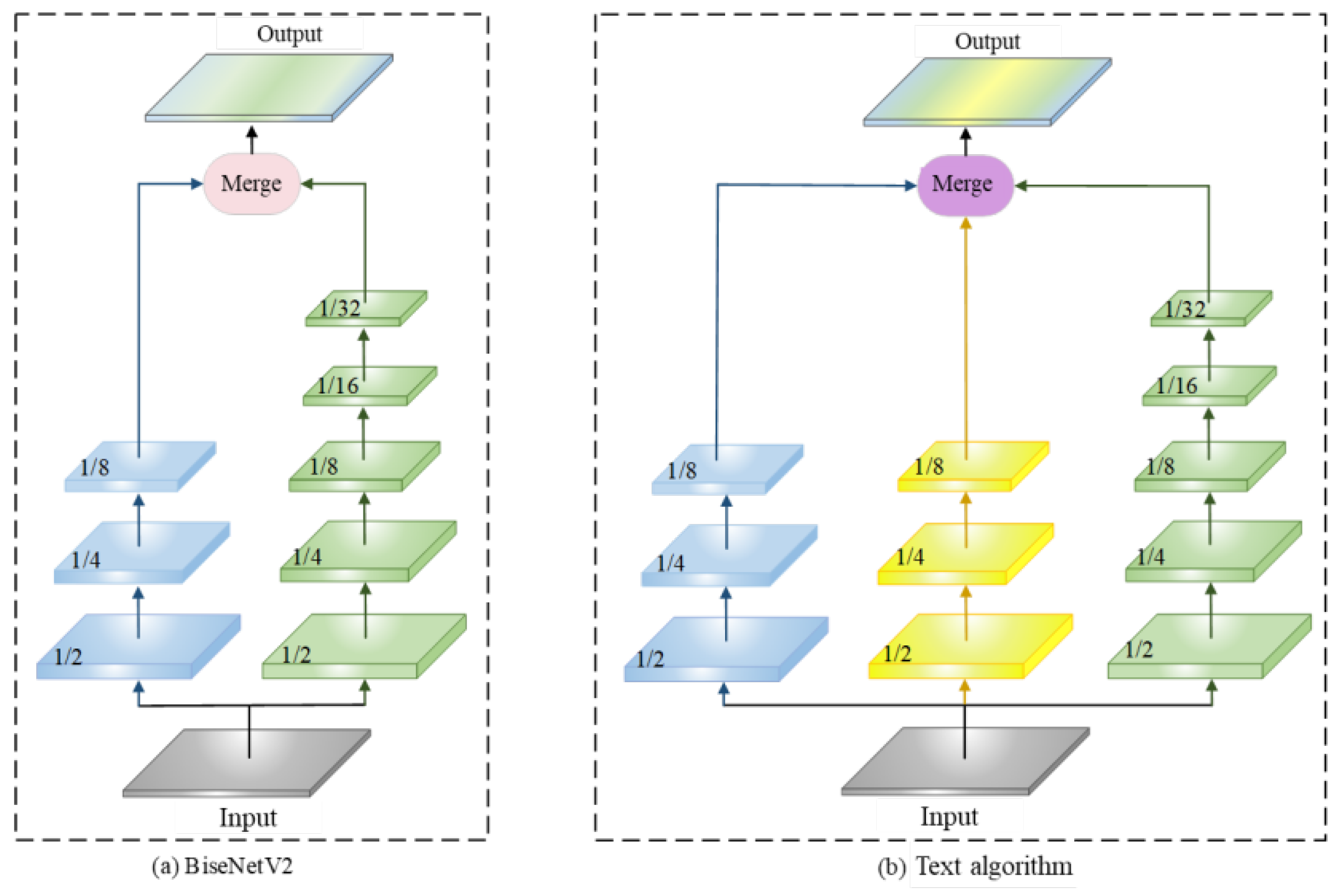
Figure 2.
Overall structure of the algorithm in this paper.
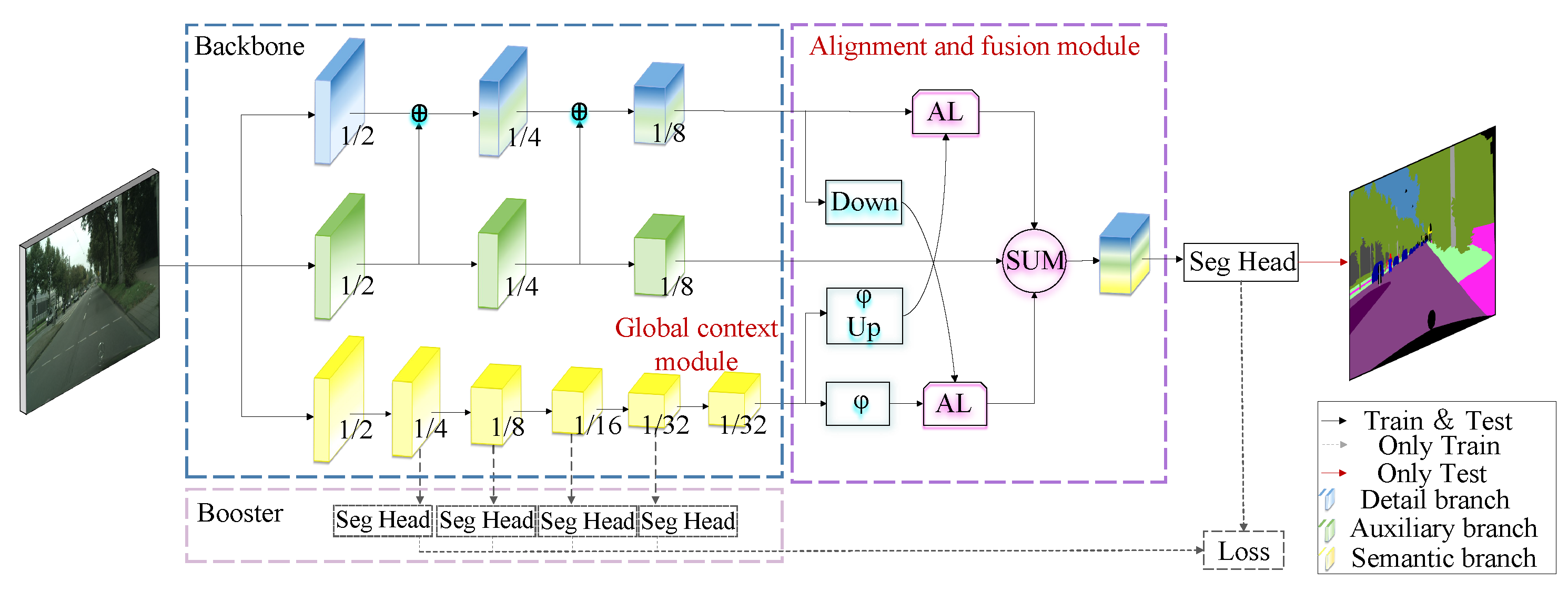
Figure 3.
Auxiliary branch structure.
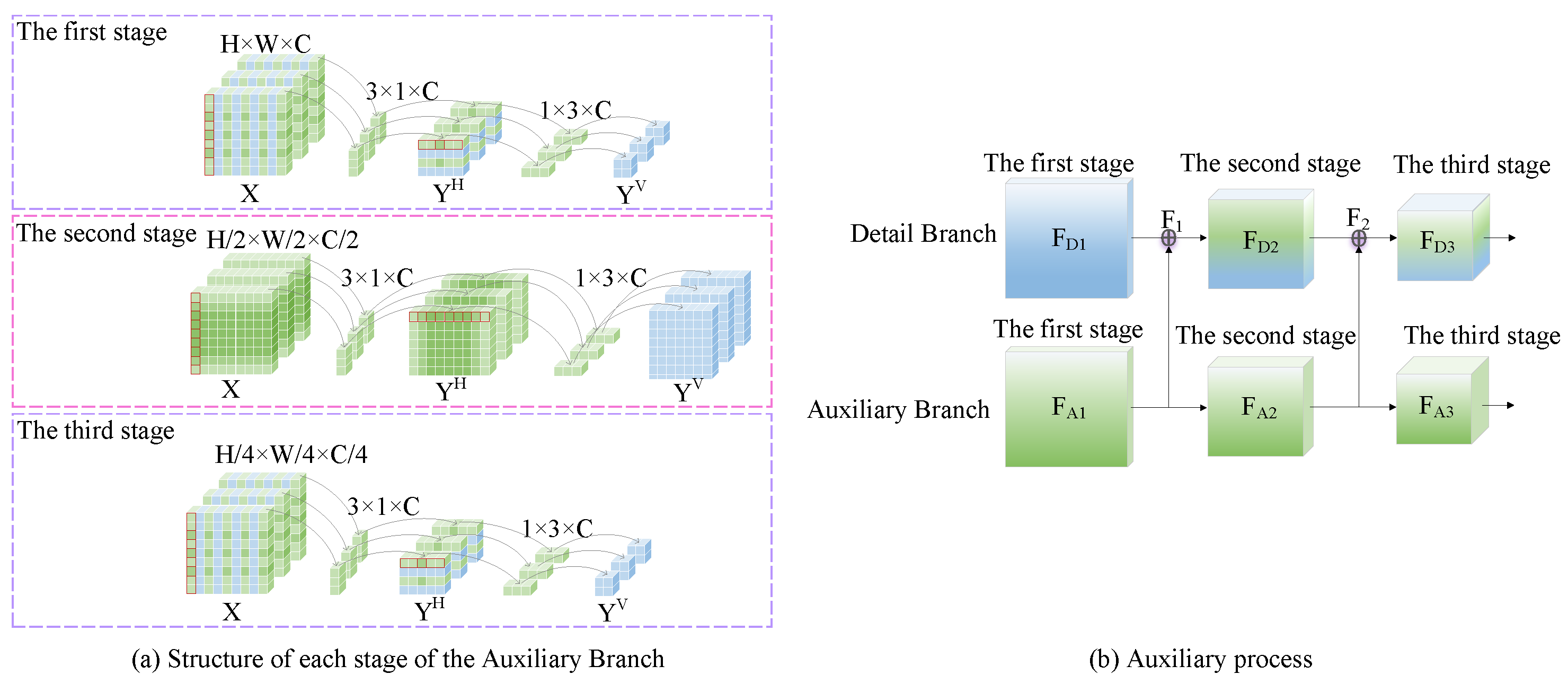
Figure 4.
Alignment and fusion module structure.

Figure 5.
Global context module.
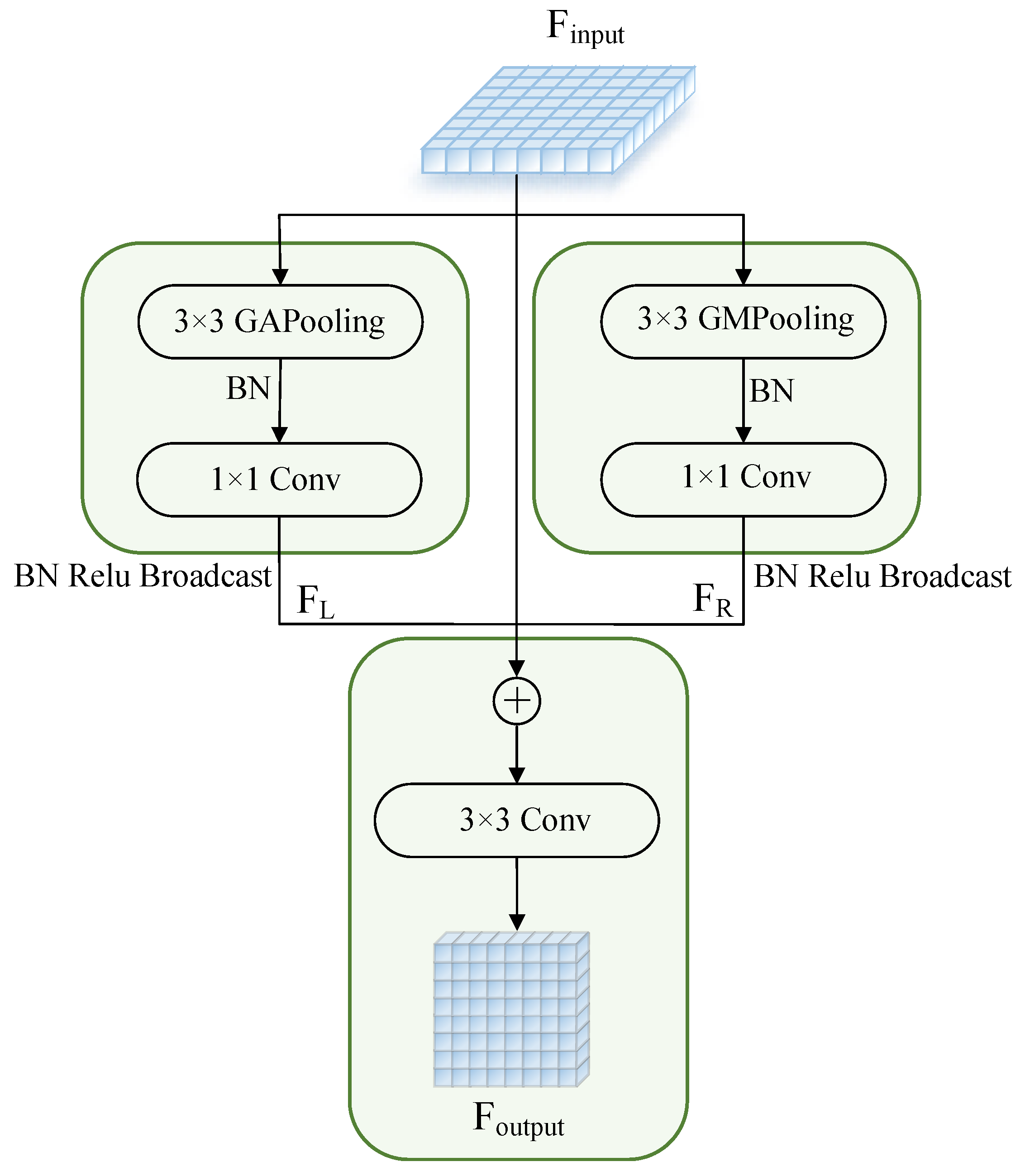
Figure 6.
Comparison of precision and speed of lightweight network.

Figure 7.
Semantic segmentation junctions of BiseNetV1, BiseNetV2 and our algorithm on Cityscapes dataset.
Figure 7.
Semantic segmentation junctions of BiseNetV1, BiseNetV2 and our algorithm on Cityscapes dataset.
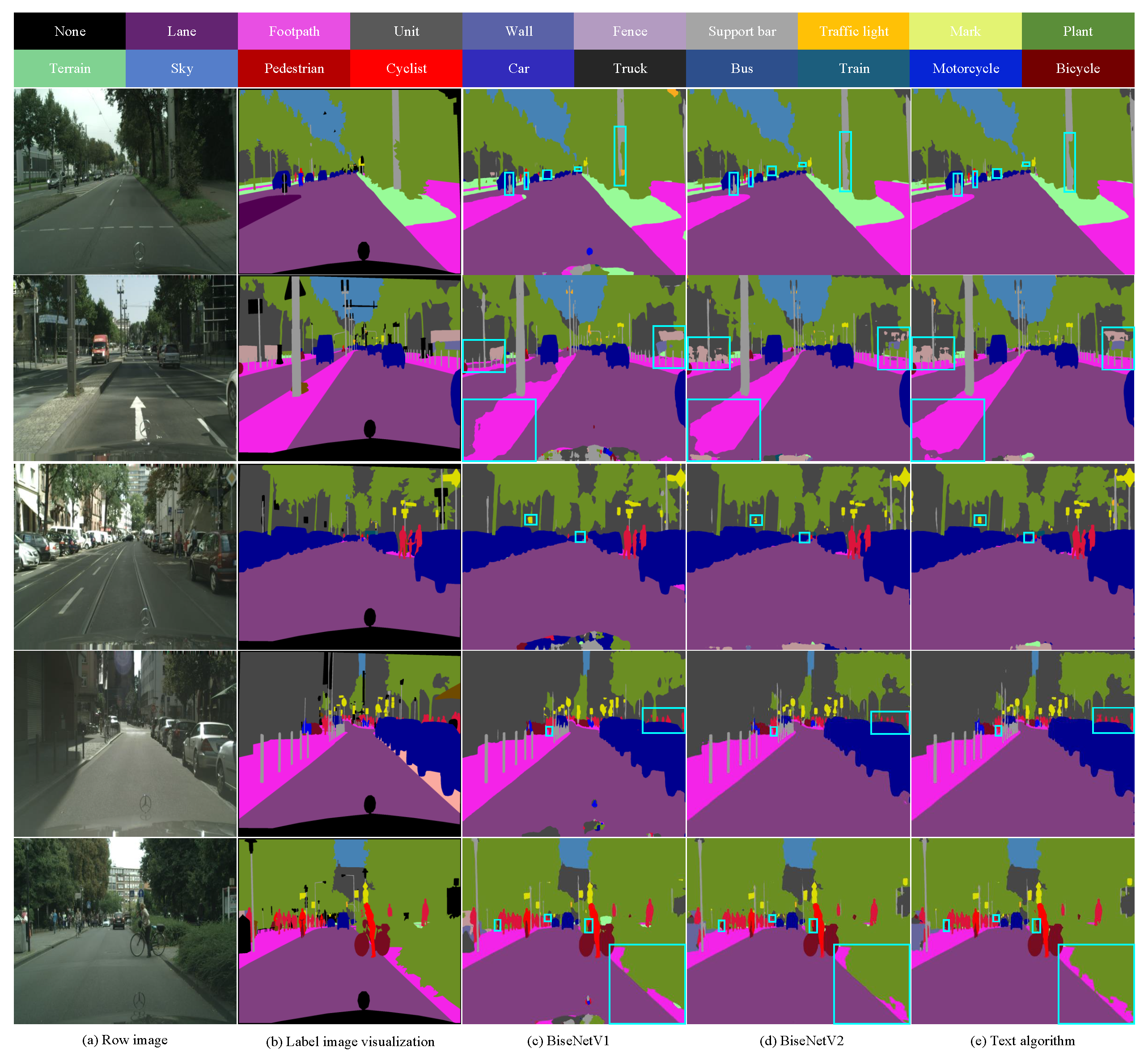
Figure 8.
Error graphs of BiseNetV1, BiseNetV2 and the algorithm in this paper on Cityscapes data set.
Figure 8.
Error graphs of BiseNetV1, BiseNetV2 and the algorithm in this paper on Cityscapes data set.
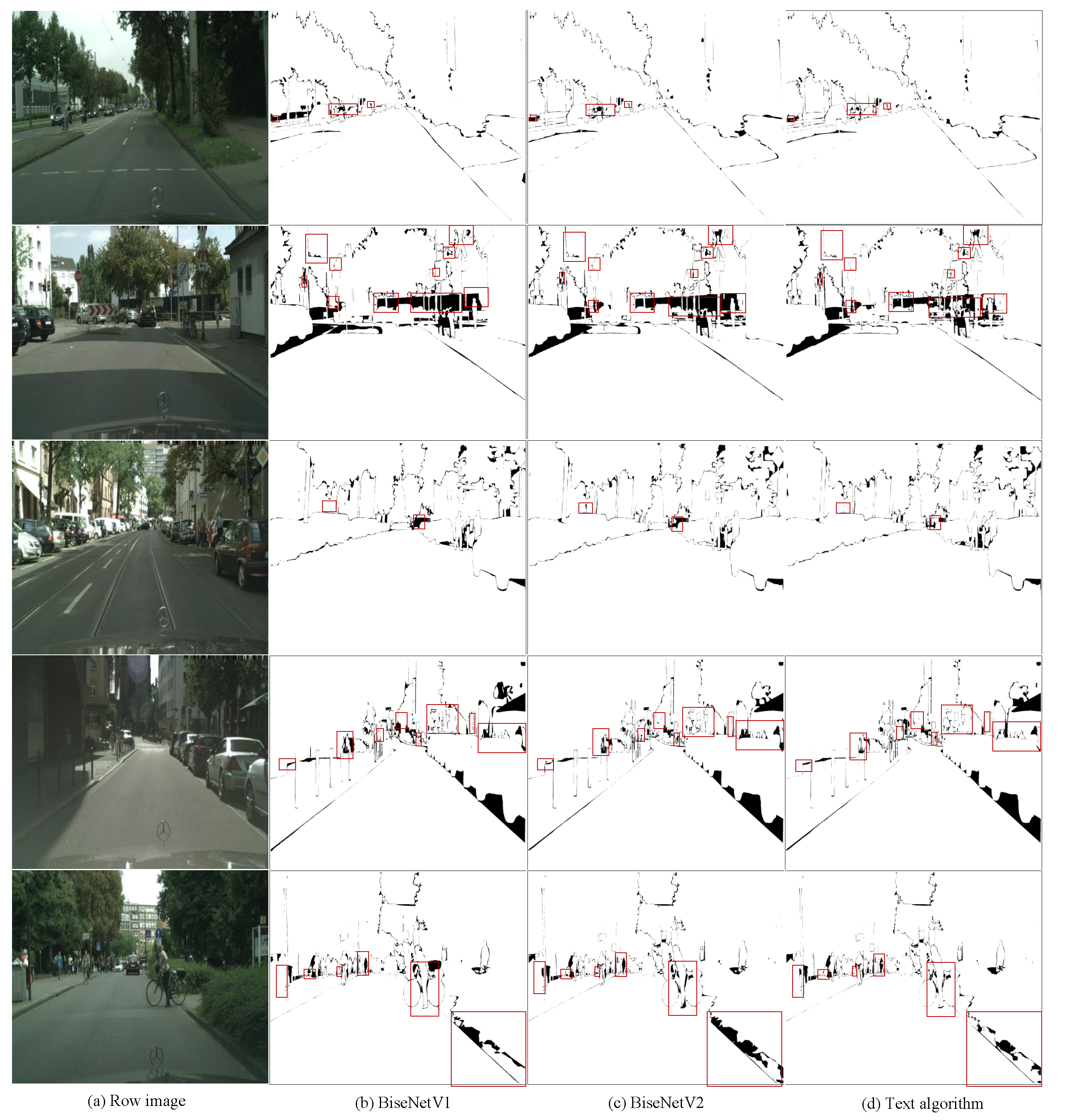
Table 1.
Results of different combinations on Cityscapes dataset.
| model | mIoU% | Running speed (Frames*s-1) | 10-6×Parameter quantity | |
|---|---|---|---|---|
| Baseline | 72.60 | 156.00 | - | |
| +Auxiliary Branch | 74.30 | 139.00 | 3.74 | |
| +AAFM | 74.40 | 137.00 | 4.25 | |
| +CGM | 73.30 | 150.00 | 3.37 | |
| +Auxiliary Branch+AAFM+CGM | 77.10 | 127.00 | 4.65 | |
Table 2.
14 algorithms compared on the Cityscapes dataset.
| Network type | Network name | Pre-training | mIoU% | Running speed (Frames*s-1) | resolution | 10-6×Parameter quantity | |
|---|---|---|---|---|---|---|---|
| Large scale | SegNet [27] | Y | 57.0 | 17 | 640×360 | 29.5 | |
| PSPNet [14] | Y | 81.2 | <1 | 713×713 | 65.7 | ||
| DeepLabV2 [16] | Y | 70.4 | <1 | 512×1024 | 44 | ||
| Light weight | Fast-SCNN [43] | N | 68 | 123.5 | 1024×2048 | 0.4 | |
| ESPNet [32] | Y | 60.3 | 112.9 | 512×1024 | 0.4 | ||
| SPANet [44] | Y | 70.6 | 92.0 | 1024×1024 | - | ||
| DFANet [45] | Y | 71.3 | 100 | 1024×2048 | 7.8 | ||
| STDC-Seg50 [46] | Y | 73.4 | 156.6 | 512×1024 | 12.3 | ||
| SGCPNet [47] | Y | 70.9 | 103.7 | 1024×2048 | 0.61 | ||
| DPFFNet [48] | N | 67.7 | 111.0 | 1024×2048 | 2.59 | ||
| SwiftNet [33] | Y | 75.4 | 39.9 | 1024×2048 | 11.8 | ||
| LCANet [24] | Y | 72.7 | 86.0 | 1024×2048 | 0.68 | ||
| BiseNetV1 [35] | Y | 68.4 | 105.8 | 786×1536 | 5.8 | ||
| BiseNetV2 [36] | N | 72.6 | 156.0 | 512×1024 | - | ||
| Ours | Y | 77.1 | 127.0 | 512×1024 | 4.65 | ||
Table 3.
Comparison of IoU% among different categories in the CityScapes dataset.
| Network name | lane | footpath | unit | wall | Fence | Support bar | Traffic light | mark | plant | topography | |
|---|---|---|---|---|---|---|---|---|---|---|---|
| SegNet [27] | 96.4 | 73.2 | 84.0 | 28.4 | 29.0 | 35.7 | 39.8 | 45.1 | 87.0 | 63.8 | |
| ENet [28] | 96.3 | 74.3 | 75.0 | 32.2 | 33.2 | 43.4 | 34.1 | 44.0 | 88.6 | 61.4 | |
| ESPNet [32] | 95.7 | 73.3 | 86.6 | 32.8 | 36.4 | 47.0 | 46.9 | 55.4 | 89.8 | 66.0 | |
| NDNet [49] | 96.6 | 75.2 | 87.2 | 44.2 | 46.1 | 29.6 | 40.4 | 53.3 | 87.4 | 57.9 | |
| LASNet [50] | 97.1 | 80.3 | 89.1 | 64.5 | 58.8 | 48.6 | 48.5 | 62.6 | 89.9 | 62.0 | |
| FSFNet [51] | 97.7 | 81.1 | 90.2 | 41.7 | 47.0 | 47.0 | 61.1 | 65.3 | 91.8 | 69.3 | |
| ERFNet [29] | 97.9 | 82.1 | 90.7 | 45.2 | 50.4 | 59.0 | 62.6 | 68.4 | 91.9 | 69.4 | |
| LEDNet [52] | 98.1 | 79.5 | 91.6 | 47.7 | 49.9 | 62.8 | 61.3 | 72.8 | 92.6 | 61.2 | |
| BisNetV2 [36] | 98.2 | 82.9 | 91.7 | 44.5 | 51.1 | 63.5 | 71.3 | 75.0 | 92.9 | 71.1 | |
| Ours | 97.9 | 83.8 | 92.3 | 63.7 | 63.8 | 64.9 | 63.1 | 77.5 | 92.4 | 63.0 |
Disclaimer/Publisher’s Note: The statements, opinions and data contained in all publications are solely those of the individual author(s) and contributor(s) and not of MDPI and/or the editor(s). MDPI and/or the editor(s) disclaim responsibility for any injury to people or property resulting from any ideas, methods, instructions or products referred to in the content. |
© 2024 by the authors. Licensee MDPI, Basel, Switzerland. This article is an open access article distributed under the terms and conditions of the Creative Commons Attribution (CC BY) license (http://creativecommons.org/licenses/by/4.0/).
Copyright: This open access article is published under a Creative Commons CC BY 4.0 license, which permit the free download, distribution, and reuse, provided that the author and preprint are cited in any reuse.


