
Submitted:
30 December 2023
Posted:
03 January 2024
You are already at the latest version
Abstract
Hyperspectral anomaly detection is to recognize anomalies from complex scene in an unsupervised way. Currently, many spectral-spatial detection methods have been proposed with a cascaded manner. However, they often neglect complementary characteristics between spectral and spatial dimensions, which easily leads to yield high false alarm rate. To alleviate this issue, a spectral-spatial information fusion (SSIF) method is designed for hyperspectral anomaly detection. First, an isolation forest is exploited to obtain spectral anomaly map, in which the object-level feature is constructed with entropy rate segmentation algorithm. Then, a local spatial saliency detection scheme is proposed to produce spatial anomaly result. Finally, the spectral and spatial anomaly scores are integrated together followed by a domain transform recursive filtering to generate the final detection result. Experiments on five hyperspectral datasets prove that the proposed SSIF produces superior detection result over other state-of-the-art detection techniques.
Keywords:
Hyperspectral image
; isolation forest
; local saliency detection
; anomaly detection
; spectralspatial fusion
1. Introduction
Hyperspectral image (HSI) contains hundreds of narrow spectral channels for each pixel, which delivers rich spectral and spatial information [1,2,3]. Owing to this virtue, HSI has been popularly employed in a considerable number of fields, such as object detection [4,5,6], image classification [7,8,9], and change detection [10,11,12]. For all application fields, hyperspectral anomaly detection, aiming to recognite the outliers whose spectra are significantly different from ambient scene, has drawn much more attention in the last few years [13].
In the last several decades, all kinds of hyperspectral anomaly detection techniques have been developed, which can be loosely grouped into several types: statistical models, subspace-based approaches, reconstruction-based approaches, and deep learning approaches. The statistical models are the most typical hyperspectral anomaly detection techniques. A representative statistical technique is the Reed-Xiaoli (RX) scheme [14], which presumes that the multivariate Gaussian distributions can be exploited to model the background and predict the probability density functions of background samples. The RX method contains two versions, i.e., local RX and global RX [15]. When the whole image is used to model Gaussian background distribution, it is named as global RX. When the RX method gauges the Gaussian model using local image pixels, it s regarded as the local RX. Nevertheless, real-world HSIs have extremely complex background, it is hard to characterize it with a multivariate Gaussian distribution. Thus, some improved versions have been studied, such as subspace RX, kernel RX, and linear filter-based RX. For example, Heesung et al. [16] developed a kernel RX detection technique, in which the hyperspectral cube was first projected into a nonlinear feature space, and then, the multivariate normal distribution was employed to fit the feature data. Guo et al. [17] developed a linear filter-based RX detection method for hyperspectral image by decreasing the weight of anomalous objects or noisy instances and enhancing one of background pixels.
The subspace-based methods postulate that the anomaly and background reflectances have high separability in a feature subspace [18,19,20]. The orthogonal subspace projection (OSP) is a classical subspace-based object detection technique. Foe instance, Chang et al. [21,22] applied an improved OSP technique for anomaly detection of hyperspectral data, where the automatic object detection process was implemented on the background pixels. Xiang et al. [23] combined local joint subspace process and classifier for hyperspectral anomaly detection. Chang et al. [24] developed a subspace selection-based isolation forest model for detecting anomaly objects in hyperspectral images which used subsampling technique rather than modeling the whole background. Furthermore, some improved detection methods have been also investigated, such as local 3D OSP [25], nonparametric OSP [26], multiple subspaces [27].
The reconstruction-based methods aim to recover the input data with a certain model, and the residual is considered as anomaly pixels. Representative reconstruction-based object detection methods mainly include low-rank representation [28,29], sparse representation (SR) [30,31], and collaborative representation [32,33]. For example, Zhu et al. [30] developed an adaptive weighted SR technique for detecting anomaly targets in hyperspectral data, in which a random selection strategy was employed to form the background dictionary. Li et al. [32] applied collaborative representation for anomaly detection of hyperspectral data, which assumes that the pixel reflectances belonging to the background area could be characterized by its adjacent pixels while the anomalous pixels cannot. Sun et al. [28] developed a low-rank and sparse matrix decomposition technique to detect the anomaly targets, where the background pixels were the low-rank part and the anomalies were thinly scattered in the whole data.
Recently, the deep learning networks have been also developed to identify the anomaly targets in hyperspectral data. Two typical unsupervised deep networks are utilized for hyperspectral anomaly detection, i.e., generative adversarial network [34,35,36] and autoencoder model [31,37,38]. For instance, Jiang et al. [34] applied generative adversarial network for detecting the anomaly objects, which assumed that the amount of background pixels was significantly greater than one of target pixels. Lu et al. [37] designed a manifold constrained autoencoder for anomaly detection of hyperspectral data, in which the manifold constraint was utilized to model the embedding representation and the autoencoder network was employed to pretain the latent intrinsic structures. In addition, some supervised deep learning networks have been also applied for detecting anomaly targets in hyperspectral data [39,40,41].
Although these approaches mentioned above use spectral and spatial information in a cascaded manner for hyperpsectral anomaly detection, they ignore the complementary property between spectral and spatial dimension. To remedy this issue, a spectral-spatial feature fusion method is proposed for hyperspectral anomaly detection, which can greatly diminish the false alarm rate by merging the spectral and spatial information. To be specific, first, a superpixel-level isolation forest method is constructed to obtain spectral anomaly score. Then, a local spatial saliency detection method is introduced to yield spatial anomaly score by using local spatial similarity in the background pixels. Finally, the spectral and spatial anomaly scores are integrated together followed by a edge-preserving filtering to generate the final detection result. Experiments on several real-world hyperspectral datasets reveal that the proposed SSIF can obtain ascendant detection results over other hyperspectral anomaly detection approaches. The key contributions of this work are concluded as follows:
1) A spectral-spatial feature fusion framework is proposed for hyperspectral anomaly detection, which makes full use of the object anomalies from both spectral and spatial diemnsions.
2) A superpixel-level isolation forest is designed to exploit the homogeneity of objects, which can well preserve the object structures.
3) Experiments on five hyperspectral data reveal that the proposed SSIF can significantly decrease the false alarm rate compared to other detection techniques.
The resting parts of this paper are grouped into five contents: Section 2 portrays the related work. Section 3 provides the detailed steps of the designed detection scheme. Section 4 analyzes the subjective and objective results of all studied methods. Section 5 provides the ablation experiments. Section 6 sums up the conclusions.
2. Related Work
2.1. Isolation Forest Algorithm
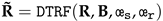
Isolation forest (iForest) was first designed for outlier detection [42]. Its core idea is that anomaly cases in a given data set are typically uncommon and distinct from regular instances, making them more prone to be separated in various binary tree architectures than the normal examples. Specifically, the input data is first separated by a randomly threshold, resulting in a tree construction from the root to the leaf. Every tree is further grown until every instance fits the predefined condition. Then, the path length, i.e., the isolation depth, of each instance is calculated with the amount of edges that the instance traverses a binary tree from the root node to the leaf node. As a result, the binary tree is recursively segmented, in which the anomalous instances arrive at leaf nodes quickly whereas normal instances must undergo many more splits before they do. In general, the path length of the anomalous instances is shoter than one of the normal instances. Finally, the anomaly value is counted by averaging the path length across multiple binary trees.
Figure 1 depicts the principle of isolation forest. As can be seen, the normal example needs more times to achieve segmentation while the anomalous example is more easily to be isolated. Accordingly, the path length of is higher than one of . Therefore, the merit of the iForest is that the outliers can be identified according to the principle of isolation tree without introducing any measurement, which can improve the computing efficiency with respect to density or distance-based detection algorithms.
2.2. Domain Transform Recursive Filtering
Domain transform recursive filtering (DTRF) is a representative edge-preserving filtering [43], which can well detach the useless information while preserve the image edges and structures. Due to this advantage, the DTRF has been generally utilized in numerous aspects, such as image interpretation, object identification, and image visualization. Assume be the input data, the transformed data is computed as:
where and mean two free parameters which are used to regulate the smoothness degree. Afterwards, the input data is further processed with recursive filter.
where indicates the filtered result of ith pixel. stands for a feedback value. b stands for the distance between and . In this work, the DTRF is denoted as , where refers to the input data, and denotes the guidance data that is utilized to the distance b.
3. Proposed Method
Figure 2 depicts the schematic of the proposed spectral-spatial information fusion detection framework, which is composed of three stages. First, the superpixel-level isolation forest is designed for calculating spectral anomaly map. Then, the spatial similarity mesaurement is employed to calculate the spatial anomaly result. Finally, the spectral and spatial anomaly scores are merged together and the DTRF is leveraged to optimize the fused map so as to generate the ultimate detection map.
3.1. Spectral Anomaly Detection
Hyperspectral image contains abundant spectral information of ground targets. The subtle spectral information provides an unique diagnostic capability for object detection. To take full advantage of the spectral information in HSIs, an object-level isolation forest is developed for spectral anomaly detection in this work, which consists of three steps: superpixel segmentation, isolation tree construction, and anomaly score estimation.
1) Superpixel segmentation: Assume be the input hyperspectral image, a principal component analysis technique is first conducted on the input data to obatin the base image , where the fist principal components are viewed as the base image. Next, the entropy rate superpixel (ERS) segmentation scheme [44] is introduced to segment the base image .
where denotes the segmentation map. represents the ERS algorithm. K is the amount of superpixels. Here, K is calculated as:
where N is an predefined parameter. denotes the proportion of nonzero elements in the binary detected map that is measured by using the Sobel filter on the base image . M stands for the amount of all pixels presented in the whole image. According to the segmentation result of the , the position location of pixels for each superpixel can be obtained. Accordingly, the 3D superpixels in HSI can be easily attained.
2) Isolation forest construction: The obtained superpixel HSI is utilized to construct isolation forest. First, T pixels are initially stochastically chosen from the input data . Then, the chosen pixels are grouped into left node and right node according to a simple decision strategy. In more detail, if is lower than the split value , the t-th pixel is grouped into the left node. On the contrary, it is grouped into the right node. Here, s denotes a random number from 1 to D. The split threshold is randomly chosen between the minimum and maximum of . Next, each child node is further segmented with the same operation above iteratively, until one of the nether conditions is required: 1) the pixels in each child node are consistent; 2) the amount of pixels in each child node is 1; 3) the number of tree comes up to the maximum height . In this paper, . At last, the procedure steps of the isolation tree are iterated q times to form the isolation forest.
3) Anomaly score estimation: The established isolation forest is exploited to gauge each pixel’s anomalyscore. Specifically, the amount of edges is considered as the path length of each pixel for every isolation tree, in which the pixel varies from the root to the terminal node. Since anomaly objects typically have relatively small areas and distinctive spectrum compared to surrounding background, they are readily segregated from external nodes. Accordingly, their path lengths are shorter while the background pixels have longer paths. Based on this observation, the path length is utilized to estimate anomalies. It is important to mention that the path length of individual pixel is dissimilar to all established trees. Thus, the eventual path length can be calculated with the averaging operation on all isolation trees.
The iForest has q isolation trees . For a test pixel , denotes the path length of x in , the avearge path length on the whole isolation trees is computed as:
Then, for test pixel x, we can compute its anomaly value as:
Here, . is set as (Euler’s constant). When the above operation is performed on each superpixel, the anomaly map can be estimalated.
3.2. Spatial Anomaly Detection
The spatial shape of the anomaly object is different from its adjacent areas [45]. Based on this observation, a local saliency measurement scheme is exploited to estimate the spatial anomaly score, which computes the spatial difference between the center pixel and its ambient background.
where is the spatial anomaly score. indicates the center window. represents the surrounding background window. W is the window size. Figure 3 presents an illustration of local saliency detection. By sliding the red window around the blue window, the local difference information between the center window and its surrounding backfround windows can be calculated. The higher the value, the more likely it is to be the background.
| Algorithm 1 Spectral-spatial feature fusion for hyperspectral anomaly detection | |
| Input: | |
| Input hyperspectral data ; | |
| Output: | |
| Detection result | |
| 1: | According to (3), calculate the 2D superpixel segmentation result |
| 2: | Calculate the corresponding 3D superpixels in HSI according to the coordinate of pixels in each 2D superpixel . |
| 3: | Construct isolation forest based on the 3D superpixel in HSI. |
| 4: | Combine the constructed forest and Eq. (6) to compute the spectral anomaly score . |
| 5: | According to Eq. (7), compute the spatial anomaly score . |
| 6: | According to Eq. (8), fuse the spectral and spatial anomaly scores to generate the fused detection result . |
| 7: | According to (9), integrate the spectral and spatial anomaly results to generate the final detection result |
| 8: | Return |
3.3. Decision Fusion
To fully utilize the complementary characteristics between spatial and spectral domains, the spectral and spatial scores are first merged together.
Then, the fused detection map is further optimized with the DTRF so as to remove the noisy pixels.
 where represents the final detection map. is the DTRF. The base image is considered as the guided image. and are fixed as 5 and 0.5, respectively.
4. Results
In this part, several experiments are designed to validate the superiority of the proposed SSIF. The recorded results are listed in the subsequent parts. All experiments are implemented on a Laptop, which is equipped with 64GB RAM and Core i9-10900K CPU.
4.1. Experimental Setup
1) Datasets: In this work, five real hyperspectral datasets from different imaging scenarios, i.e., Beach, Pavia city, San Diego-I, San Diego-II, and Gulfport, are exploited to judge the detection effect of all considered techniques, which are introduced as follows:
The Beach data was gained by the Airborne Visible/Infrared Imaging Spectrometer (AVIRIS) device over Cat Island. This data embodies 224 reflectance channels varying from 0.4-2.5m. Before experiments, several water absorption and noisy channels are removed, and 188 channels are preserved. Its size is of 150×150 and each pixel accounts for 17.2 m. Figure 4 presents the pseudocolor image and reference map.
The Pavia city data was collected by the Reflective Optics System Imaging Spectrometer (ROSIS) equipment. It is about Pavia city scene. This data is of 150×150 pixels with sptial resolution 1.3 m. The imaging range is from 0.43 to 0.86 m with 205 spectral bands. This scene has water, bridge, bare soil, and buildings. The pseudocolor RGB and reference image are depicted in Figure 5.
San Diego-I dataset was acquired by the AVIRIS device over the airport region of San Diego, USA. This data’s spatial size is 100×100 pixels and each pixel accounts for 3.5 m. The imaging scope varies from 0.4 to 2.5m with spectral interval of 10 nm. After discarding water absorption and noisy channels, 189 channels are employed for experiments. Figure 6 gives the pseudocolor image and reference image.
San Diego-II dataset is situated at the heart of the airport area of San Diego, which is named as San Diego-II. The spatial size of this data is 100×100. This scene is composed of exposed soil, hangers, parking aprons, and airports, in which three airports are taken as anomalies. Figure 7 gives the pseudocolor image and ground truth.
The Gulfport data was obtained by the AVIRIS device about the airport region of Gulfport, USA. This image contains 191 spectral channels varying from 0.55 to 1.85 m. Its spatial size is of 100 × 100 pixels and each pixel accounts for 3.4 m. This data has highway, airport runway, vegetation, and airport. The airport is considered as anomalies. Figure 8 depicts the sample image and reference image.
2) Objective Indexes: To quantitatively assess the detection effect of different methods, two widely used metrics are adopted, i.e., ROC curve and AUC. The ROC curve provides the correlation between the detection probability (DP) and the false alarm rate (FAR) at different threhold settings. In more detail, when the detection result and the reference image are given, the DP and FAR are calculated as:
where means the amount of identified object pixels below a fixed threshold. means the total amount of true object region in the original dataset. indicates the sum of false alarm pixels. N indicates the sum of pixels in the input image. When the DP value is higher than one of other approaches at the same false alarm, it means that this method with higher DP yields the best detection result.
The AUC value is estimated with the whole region under ROC curve. A higher AUC represents a better anomaly detection result. The AUC is given by:
where denots how many corrent positive samples occur among all examples when the threhold is H. records how many incorrect positive samples occur among all negative examples.
4.2. Detection Results
To illustrate the strength of the proposed SSIF, several hyperspectral anomaly detection techniques are selected as compared techniques, including RX [14], CRD [32], AED [46], KIFD [47], PTA [48], RGAE [49], and SSIIF [50]. These approaches are adopted since they are representative or recently developed techniques. Specifically, the RX is a classical statistical modeling technique. The CRD is a popular collaborative representation scheme. The AED is based on attribute filters. The PTA is tensor representation technique. The KIFD and SSIIF are the representative iForest methods. The RGAE is based on graph autoencoder model. The realted parameters in these detection methods follow the corresponding publication.
Figure 9, Figure 10, Figure 11, Figure 12 and Figure 13 depict the detection results of all techniques on five datasets. It can be found that the RX scheme yields unsatisfactory detection maps. Many anomalies cannot be well detected in the resulting maps. For example, the RX method fails to identify three airplanes for San Diego-I dataset. For the CRD scheme, the abnormal objects are hardly detected. The background information is regarded as the anomalies. For the AED method, although the anomalies can be effectively detected, the similar land covers in the background also are viewed as anomalies. For example, the island in the Beach dataset is mistakenly detected. The KIFD and PTA techniques can well detect the locations and shapes of different objects. However, they obtains very high false alarm rate for all datasets. The reason is that the KIFD and PTA methods fail to removes the interference of the background information. The RGAE method suffers from poor detection performance. The airplanes in the San Diego-I, San Diego-II, and Gulfport datasets cannot effectively detected. the SSIIF method slightly improves the detection performance. Nevertheless, the background information still can be found in the detection results. By constrast, the proposed SSIF yields the best detection maps with lowest false alarm rate among all considered approaches. The background information can be well suppressed and only anomalies are effectively seperated from the original image.
Furthermore, the objective detection performances of different approaches are quantitatively assessed via the AUC score. Table 1 lists the AUC scores of all studied detection approaches. The best detection score in each row is displayed in bold. It is obvious that the proposed SSIF produces the highest AUCs on all images. This also illustrates that the proposed method indeed yields the best detection effect compared to other techniques. The RGAE method cannot achieve stable detection results. For the San Diego-I and Gulfport datasets, the RGAE methpd yields the lowest AUCs. Moreover, the RX and CRD methods also obtain relatively low detection accuracy. Generally, among all studied detection techniques, the proposed SSIF achieves the highest objective accuracy and produces satisfactory detection results.
Figure 14 depicted the ROC curves of all detection approaches on all images. It can be observed that the detection probability of the proposed SSIF is always greater than other compared techniques when the FAR is varying from 0 to 1. This proclaims that the proposed SSIF yields superior detection results among all detection approaches. For SanDiego-II dataset, the proposed SSIF is slightly lower probability of detection than the RGAE method when the FAR is from 0.05 to 0.1. In general, by observing the ROC curves of Figure 14, it is obvious that the designed SSIF is higher than other approaches.
5. Discussion
5.1. The Influence of Different Parameters
In this subsection, the influence of all free parameters in the spectral anomaly detection branch, i.e., the amount of trees q and the amount of superpixels N, to the detection effect of the proposed method is discussed. Figure 15 (a) depicts the influence of different numbers of isolation tress. It can be found that when the amount of isolation trees is relatively small, the proposed SSIF produces low detection accuracy. When the amount of isolation trees is greater than 50, the detection effect is satisfactory. Furthermore, as the increase of the amount of isolation trees, the computing cost of the proposed framework has an increasing trend. In this work, the amount of isolation trees q is set as 50. Besides, Figure 15 (b) presents the AUCs of the proposed SSIF with different numbers of superpixels. It is shown that when the number of superpixels is relatively large, the detection accuracy tends to decrease. The reason is that excessive superpixels lead to image oversegmentation issue. In addition, a quantity of superpixels cause each local region containing fewer pixels, resulting in unstable detection results. In this work, the number of superpixels N is set as 9 for all experiments.
The window size W in the spatial anomaly detection branch also needs to be determined. Figure 16 depicts the detection accuracy of different sizes of window in the spatial anomaly detection branch. The window size W is varying from 1 to 13 with step size 2. When the window size W increases, the AUC of the proposed SSIF tends to decrease. This is because useless spatial information is used to measure the difference between the center window and the local window. By observing Figure 16, it is obvious that when the window size W is 3, the detection effect of the proposed method is the highest. Thus, the window size W is set as 3 for following experiments.
5.2. The Influence of Different Components
In this part, the influence of different components in the proposed framework to the detection performance is anlyzed. Table 2 lists the quantative scores of different components in the developed framework. By comparing the spatial branch and spectral branch, it is shown that the spectral branch yields lower detection accuracy. The reason is that hyperspectral image usually suffers from spectral mixture issue. By fusing the spectral and spatial branches, the detection accuracy gains great improvement. For example, the AUC value of the proposed SSIF is increased by 1.92% than one of the spectral branch. This experiment also illustrates that the spectral and spatial information fusion can well boost the detection effect.
5.3. Computing Time
In this part, the running time of different detection schemes on all datasets is discussed. Table 3 presents the computational cost of all detection schemes. It is shown that the RX detector perform the fastest. The reason is that this method only requires simple distance calculation. However, the RX method produces relatively poor detection result. The computational burden of the RGAE scheme is highest among all studied techniques since the autoencoders require a plentiful of iterations during the training process. By constrast, the running time of the proposed SSIF is quite competitive among all studied techniques. Furthermore, as the increase of the spatial size, the computational cost tends to increase. How to decrease the computing time is still an interesting topic.
6. Conclusions
In this study, a spectral-spatial feature fusion is designed for hyperspectral anomaly detection, which is comprised of three main stages. First, an object-level isolation forest is constructed to estimate the spectral anomaly score. Then, a local spatial similarity strategy is exploited to produce the spatial anomaly score. Finally, the spectral and spatial anomaly probabilitity maps are merged together followed by a edge-preserving filtering to yiled the ultimate detection map. Experiments on five real-world hyperspectral datasets verify that the proposed SSIF can obtain better detection results with respect to other hyperspectral anomaly detection approaches. In addition, the proposed SSIF can well suppress the background information and achieves a substantially lower false alarm rate. In the future, we will focus on developing real-time hyperspectral anomaly detection techniques. Furthermore, we will expand the applications of hyperspectral anomaly detection. For example, we can combine it with point target detection so as to achieve infrared dim small flying target recognition [51].
Author Contributions
S. L. conducted the experiments and wrote this manuscript. Z. Li designed the detection framework. Y. Wang and X. Qiu provided useful comments. T. Liu and D. Zhang carefully revised this manuscript. J. Cao provided instructive suggestions.
Funding
This work was supported in part by the National Natural Science Foundation of China (Grant No. 62201207).
Abbreviations
The following abbreviations are used in this manuscript:
| SSIF | Spectral-spatial information fusion |
| HSI | Hyperspectral image |
| RX | Reed-Xiaoli |
| OSP | Orthogonal subspace projection |
| SR | Sparse representation |
| iForest | Isolation forest |
| DTRF | Domain transform recursive filtering |
| ERS | Entropy rate superpixel |
| AVIRIS | Airborne Visible/Infrared Imaging Spectrometer |
| ROSIS | Reflective Optics System Imaging Spectrometer |
| CRD | Collaborative representation-based detector |
| AED | Attribute and edge-preserving filtering-based method |
| KIFD | Kernel isolation forest-based method |
| PTA | Prior-based tensor approximation |
| RGAE | Robust graph autoencoders |
References
- Zhang, W.; Guo, H.; Liu, S.; Wu, S. Attention-Aware Spectral Difference Representation for Hyperspectral Anomaly Detection. Remote Sensing 2023, 15, 2652. [Google Scholar] [CrossRef]
- Duan, P.; Hu, S.; Kang, X.; Li, S. Shadow Removal of Hyperspectral Remote Sensing Images With Multiexposure Fusion. IEEE Transactions on Geoscience and Remote Sensing 2022, 60, 1–11. [Google Scholar] [CrossRef]
- Kang, X.; Wang, Z.; Duan, P.; Wei, X. The Potential of Hyperspectral Image Classification for Oil Spill Mapping. IEEE Transactions on Geoscience and Remote Sensing 2022, 60, 1–15. [Google Scholar] [CrossRef]
- Wang, H.; Yang, M.; Zhang, T.; Tian, D.; Wang, H.; Yao, D.; Meng, L.; Shen, H. Hyperspectral Anomaly Detection with Differential Attribute Profiles and Genetic Algorithms. Remote Sensing 2023, 15, 1050. [Google Scholar] [CrossRef]
- Zhang, X.; Xie, W.; Li, Y.; Lei, J.; Du, Q. Filter Pruning via Learned Representation Median in the Frequency Domain. IEEE Transactions on Cybernetics 2023, 53, 3165–3175. [Google Scholar] [CrossRef] [PubMed]
- Liu, Y.; Xie, W.; Li, Y.; Li, Z.; Du, Q. Dual-Frequency Autoencoder for Anomaly Detection in Transformed Hyperspectral Imagery. IEEE Transactions on Geoscience and Remote Sensing 2022, 60, 1–13. [Google Scholar] [CrossRef]
- Duan, P.; Kang, X.; Li, S.; Ghamisi, P.; Benediktsson, J.A. Fusion of Multiple Edge-Preserving Operations for Hyperspectral Image Classification. IEEE Transactions on Geoscience and Remote Sensing 2019, 57, 10336–10349. [Google Scholar] [CrossRef]
- Zhang, Y.; Duan, P.; Mao, J.; Kang, X.; Fang, L.; Ghamisi, P. Contour Structural Profiles: An Edge-Aware Feature Extractor for Hyperspectral Image Classification. IEEE Transactions on Geoscience and Remote Sensing 2022, 60, 1–14. [Google Scholar] [CrossRef]
- Taskin, G.; Yetkin, E.F.; Camps-Valls, G. A Scalable Unsupervised Feature Selection With Orthogonal Graph Representation for Hyperspectral Images. IEEE Transactions on Geoscience and Remote Sensing 2023, 61, 1–13. [Google Scholar] [CrossRef]
- Hasanlou, M.; Seydi, S.T. Hyperspectral change detection: An experimental comparative study. International journal of remote sensing 2018, 39, 7029–7083. [Google Scholar] [CrossRef]
- Hou, Z.; Li, W.; Li, L.; Tao, R.; Du, Q. Hyperspectral change detection based on multiple morphological profiles. IEEE Transactions on Geoscience and Remote Sensing 2021, 60, 1–12. [Google Scholar] [CrossRef]
- Eismann, M.T.; Meola, J.; Hardie, R.C. Hyperspectral change detection in the presenceof diurnal and seasonal variations. IEEE Transactions on Geoscience and Remote Sensing 2007, 46, 237–249. [Google Scholar] [CrossRef]
- Su, H.; Wu, Z.; Zhang, H.; Du, Q. Hyperspectral anomaly detection: A survey. IEEE Geoscience and Remote Sensing Magazine 2021, 10, 64–90. [Google Scholar] [CrossRef]
- Reed, I.S.; Yu, X. Adaptive multiple-band CFAR detection of an optical pattern with unknown spectral distribution. IEEE transactions on acoustics, speech, and signal processing 1990, 38, 1760–1770. [Google Scholar] [CrossRef]
- Kwon, H.; Der, S.Z.; Nasrabadi, N.M. Adaptive anomaly detection using subspace separation for hyperspectral imagery. Optical Engineering 2003, 42, 3342–3351. [Google Scholar] [CrossRef]
- Kwon, H.; Nasrabadi, N. Kernel RX-algorithm: a nonlinear anomaly detector for hyperspectral imagery. IEEE Transactions on Geoscience and Remote Sensing 2005, 43, 388–397. [Google Scholar] [CrossRef]
- Guo, Q.; Zhang, B.; Ran, Q.; Gao, L.; Li, J.; Plaza, A. Weighted-RXD and Linear Filter-Based RXD: Improving Background Statistics Estimation for Anomaly Detection in Hyperspectral Imagery. IEEE Journal of Selected Topics in Applied Earth Observations and Remote Sensing 2014, 7, 2351–2366. [Google Scholar] [CrossRef]
- Tan, K.; Hou, Z.; Wu, F.; Du, Q.; Chen, Y. Anomaly detection for hyperspectral imagery based on the regularized subspace method and collaborative representation. Remote sensing 2019, 11, 1318. [Google Scholar] [CrossRef]
- Wang, L.; Chang, C.I.; Lee, L.C.; Wang, Y.; Xue, B.; Song, M.; Yu, C.; Li, S. Band subset selection for anomaly detection in hyperspectral imagery. IEEE Transactions on Geoscience and Remote Sensing 2017, 55, 4887–4898. [Google Scholar] [CrossRef]
- Lo, E. Maximized subspace model for hyperspectral anomaly detection. Pattern Analysis and Applications 2012, 15, 225–235. [Google Scholar] [CrossRef]
- Chang, C.I.; Cao, H.; Song, M. Orthogonal Subspace Projection Target Detector for Hyperspectral Anomaly Detection. IEEE Journal of Selected Topics in Applied Earth Observations and Remote Sensing 2021, 14, 4915–4932. [Google Scholar] [CrossRef]
- Chang, C.I.; Cao, H.; Chen, S.; Shang, X.; Yu, C.; Song, M. Orthogonal Subspace Projection-Based Go-Decomposition Approach to Finding Low-Rank and Sparsity Matrices for Hyperspectral Anomaly Detection. IEEE Transactions on Geoscience and Remote Sensing 2021, 59, 2403–2429. [Google Scholar] [CrossRef]
- Xiang, P.; Zhou, H.; Li, H.; Song, S.; Tan, W.; Song, J.; Gu, L. Hyperspectral anomaly detection by local joint subspace process and support vector machine. International Journal of Remote Sensing 2020, 41, 3798–3819. [Google Scholar] [CrossRef]
- Chang, S.; Du, B.; Zhang, L. A subspace selection-based discriminative forest method for hyperspectral anomaly detection. IEEE Transactions on Geoscience and Remote Sensing 2020, 58, 4033–4046. [Google Scholar] [CrossRef]
- Zhang, X.; Wen, G. A hyperspectral imagery anomaly detection algorithm based on local three-dimensional orthogonal subspace projection. Image and Signal Processing for Remote Sensing XXI. SPIE, 2015, Vol. 9643, pp. 600–607.
- Matteoli, S.; Acito, N.; Diani, M.; Corsini, G. Subspace based non-parametric approach for hyperspectral anomaly detection in complex scenarios. Image and Signal Processing for Remote Sensing XX. SPIE, 2014, Vol. 9244, pp. 245–253.
- Song, S.; Zhou, H.; Zhou, J.; Qian, K.; Cheng, K.; Zhang, Z. Hyperspectral anomaly detection based on anomalous component extraction framework. Infrared Physics & Technology 2019, 96, 340–350. [Google Scholar]
- Sun, W.; Liu, C.; Li, J.; Lai, Y.M.; Li, W. Low-rank and sparse matrix decomposition-based anomaly detection for hyperspectral imagery. Journal of Applied Remote Sensing 2014, 8, 083641–083641. [Google Scholar] [CrossRef]
- Yang, Y.; Zhang, J.; Song, S.; Liu, D. Hyperspectral anomaly detection via dictionary construction-based low-rank representation and adaptive weighting. Remote sensing 2019, 11, 192. [Google Scholar] [CrossRef]
- Zhu, L.; Wen, G. Hyperspectral anomaly detection via background estimation and adaptive weighted sparse representation. Remote Sensing 2018, 10, 272. [Google Scholar] [CrossRef]
- Zhao, R.; Du, B.; Zhang, L. Hyperspectral anomaly detection via a sparsity score estimation framework. IEEE Transactions on Geoscience and Remote Sensing 2017, 55, 3208–3222. [Google Scholar] [CrossRef]
- Li, W.; Du, Q. Collaborative representation for hyperspectral anomaly detection. IEEE Transactions on Geoscience and Remote Sensing 2014, 53, 1463–1474. [Google Scholar] [CrossRef]
- Vafadar, M.; Ghassemian, H. Anomaly detection of hyperspectral imagery using modified collaborative representation. IEEE Geoscience and Remote Sensing Letters 2018, 15, 577–581. [Google Scholar] [CrossRef]
- Jiang, T.; Li, Y.; Xie, W.; Du, Q. Discriminative reconstruction constrained generative adversarial network for hyperspectral anomaly detection. IEEE Transactions on Geoscience and Remote Sensing 2020, 58, 4666–4679. [Google Scholar] [CrossRef]
- Jiang, K.; Xie, W.; Li, Y.; Lei, J.; He, G.; Du, Q. Semisupervised Spectral Learning With Generative Adversarial Network for Hyperspectral Anomaly Detection. IEEE Transactions on Geoscience and Remote Sensing 2020, 58, 5224–5236. [Google Scholar] [CrossRef]
- Xie, W.; Liu, B.; Li, Y.; Lei, J.; Chang, C.I.; He, G. Spectral Adversarial Feature Learning for Anomaly Detection in Hyperspectral Imagery. IEEE Transactions on Geoscience and Remote Sensing 2020, 58, 2352–2365. [Google Scholar] [CrossRef]
- Lu, X.; Zhang, W.; Huang, J. Exploiting embedding manifold of autoencoders for hyperspectral anomaly detection. IEEE Transactions on Geoscience and Remote Sensing 2019, 58, 1527–1537. [Google Scholar] [CrossRef]
- Zhang, L.; Cheng, B. A stacked autoencoders-based adaptive subspace model for hyperspectral anomaly detection. Infrared Physics & Technology 2019, 96, 52–60. [Google Scholar]
- Li, W.; Wu, G.; Du, Q. Transferred Deep Learning for Anomaly Detection in Hyperspectral Imagery. IEEE Geoscience and Remote Sensing Letters 2017, 14, 597–601. [Google Scholar] [CrossRef]
- Ma, N.; Peng, Y.; Wang, S.; Liu, D. Hyperspectral image anomaly targets detection with online deep learning. 2018 IEEE International Instrumentation and Measurement Technology Conference (I2MTC), 2018, pp. 1–6.
- Song, S.; Zhou, H.; Yang, Y.; Song, J. Hyperspectral Anomaly Detection via Convolutional Neural Network and Low Rank With Density-Based Clustering. IEEE Journal of Selected Topics in Applied Earth Observations and Remote Sensing 2019, 12, 3637–3649. [Google Scholar] [CrossRef]
- Liu, F.T.; Ting, K.M.; Zhou, Z.H. Isolation-based anomaly detection. ACM Transactions on Knowledge Discovery from Data (TKDD) 2012, 6, 1–39. [Google Scholar] [CrossRef]
- Gastal, E.S.; Oliveira, M.M. Domain transform for edge-aware image and video processing. In ACM SIGGRAPH 2011 papers; 2011; pp. 1–12.
- Liu, M.Y.; Tuzel, O.; Ramalingam, S.; Chellappa, R. Entropy-Rate Clustering: Cluster Analysis via Maximizing a Submodular Function Subject to a Matroid Constraint. IEEE Transactions on Pattern Analysis and Machine Intelligence 2014, 36, 99–112. [Google Scholar] [CrossRef]
- Ju, H.; Liu, Z.; Wang, Y. Ju, H.; Liu, Z.; Wang, Y. Hyperspetral anomaly detection incorporating spatial information. 2018 Eighth International Conference on Image Processing Theory, Tools and Applications (IPTA). IEEE, 2018, pp. 1–5.
- Kang, X.; Zhang, X.; Li, S.; Li, K.; Li, J.; Benediktsson, J.A. Hyperspectral Anomaly Detection With Attribute and Edge-Preserving Filters. IEEE Transactions on Geoscience and Remote Sensing 2017, 55, 5600–5611. [Google Scholar] [CrossRef]
- Li, S.; Zhang, K.; Duan, P.; Kang, X. Hyperspectral Anomaly Detection With Kernel Isolation Forest. IEEE Transactions on Geoscience and Remote Sensing 2020, 58, 319–329. [Google Scholar] [CrossRef]
- Li, L.; Li, W.; Qu, Y.; Zhao, C.; Tao, R.; Du, Q. Prior-Based Tensor Approximation for Anomaly Detection in Hyperspectral Imagery. IEEE Transactions on Neural Networks and Learning Systems 2022, 33, 1037–1050. [Google Scholar] [CrossRef]
- Fan, G.; Ma, Y.; Mei, X.; Fan, F.; Huang, J.; Ma, J. Hyperspectral Anomaly Detection With Robust Graph Autoencoders. IEEE Transactions on Geoscience and Remote Sensing 2022, 60, 1–14. [Google Scholar] [CrossRef]
- Song, X.; Aryal, S.; Ting, K.M.; Liu, Z.; He, B. Spectral–Spatial Anomaly Detection of Hyperspectral Data Based on Improved Isolation Forest. IEEE Transactions on Geoscience and Remote Sensing 2022, 60, 1–16. [Google Scholar] [CrossRef]
- QIAO Mengyu, TAN Jinlin, L. Y.X.Q.W.S. Infrared Dim Small Flying Target Recognition Algorithm for Space-Based Surveillance. Chinese Space Science and Technology 2022, 42, 125. [Google Scholar]
Figure 1.
Principle of the isolation forest. (a) Anomalous example is isolated with four segmentations. (b) Normal example is isolated with thirteen segmentations.
Figure 1.
Principle of the isolation forest. (a) Anomalous example is isolated with four segmentations. (b) Normal example is isolated with thirteen segmentations.
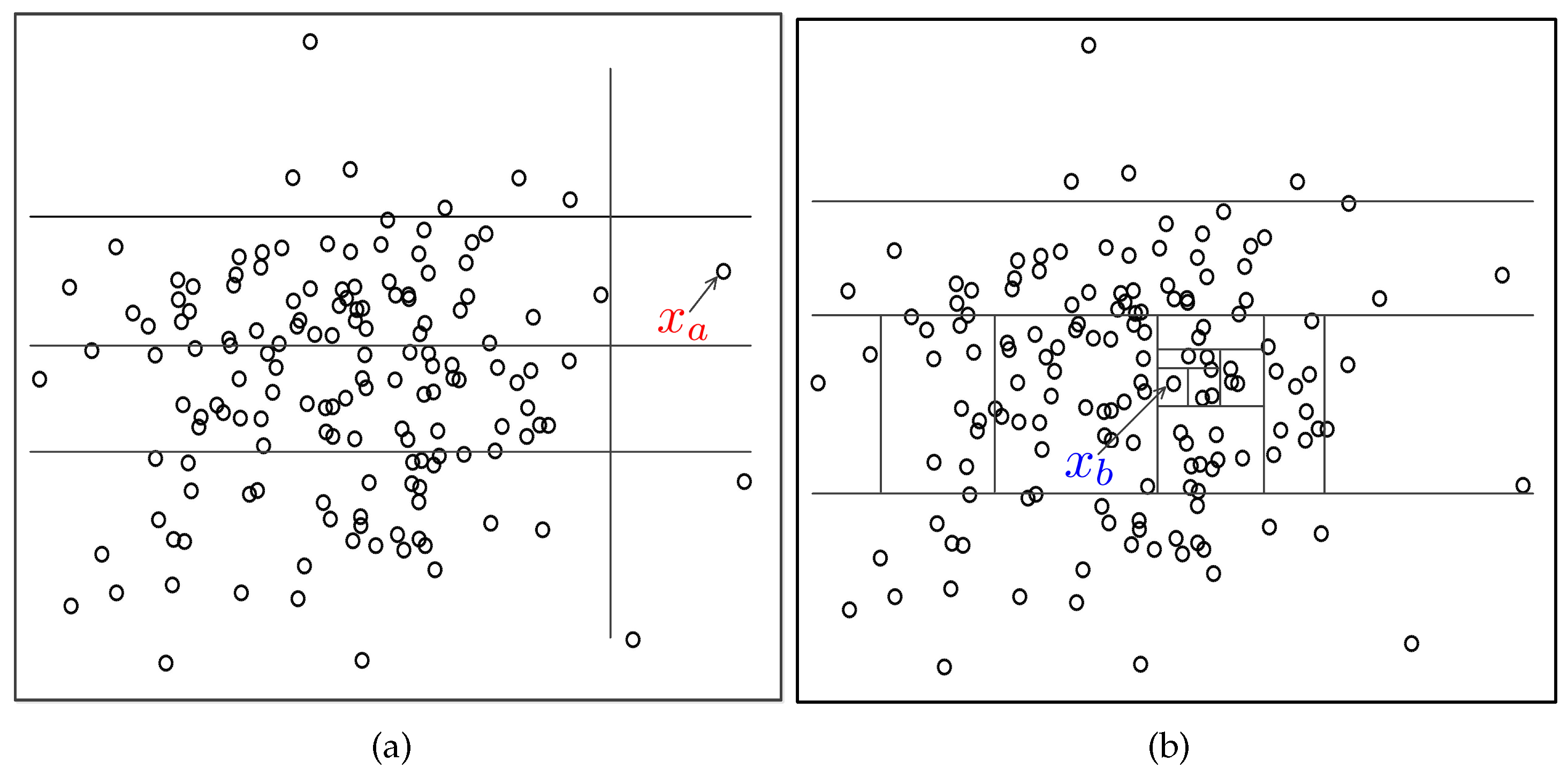
Figure 2.
The schematic of the SSIF detection method.
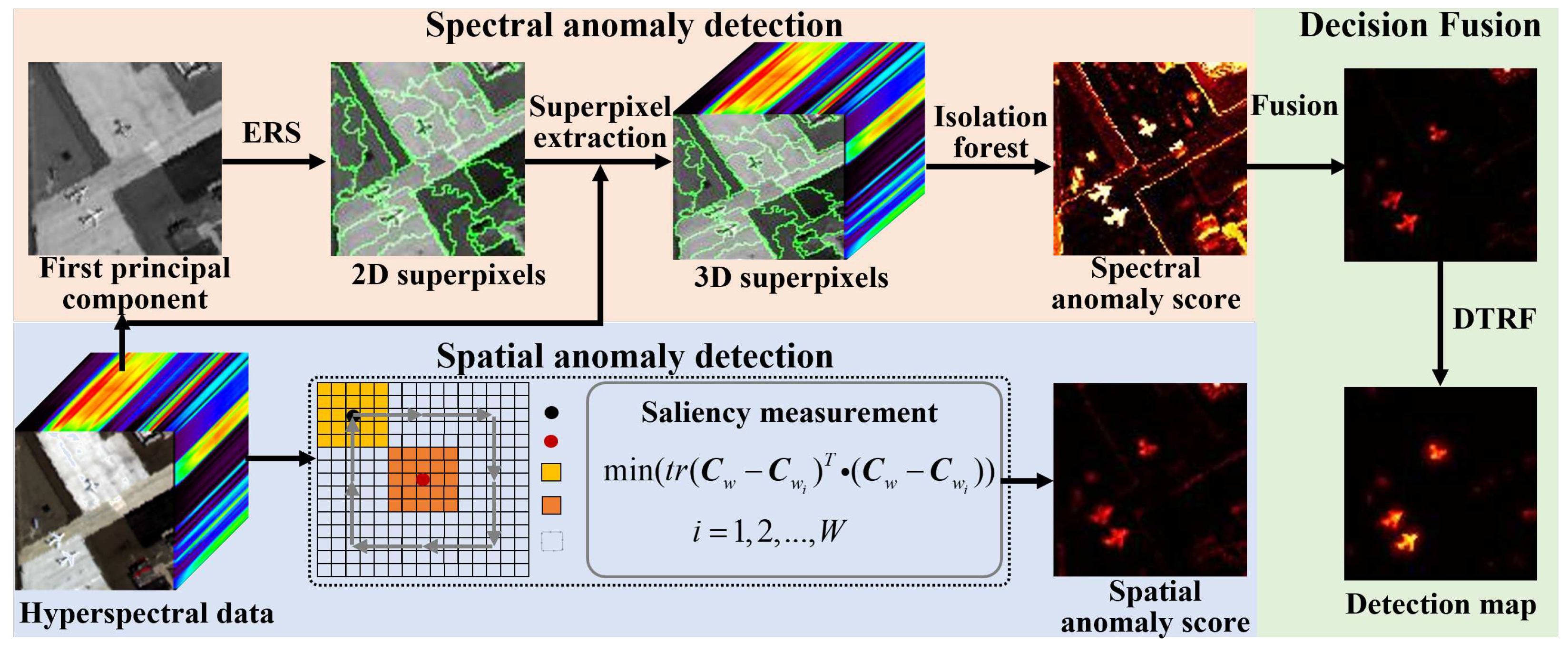
Figure 3.
An illustration of local saliency detection.
Figure 4.
Beach dataset. (a) RGB composite image. (b) Ground truth.
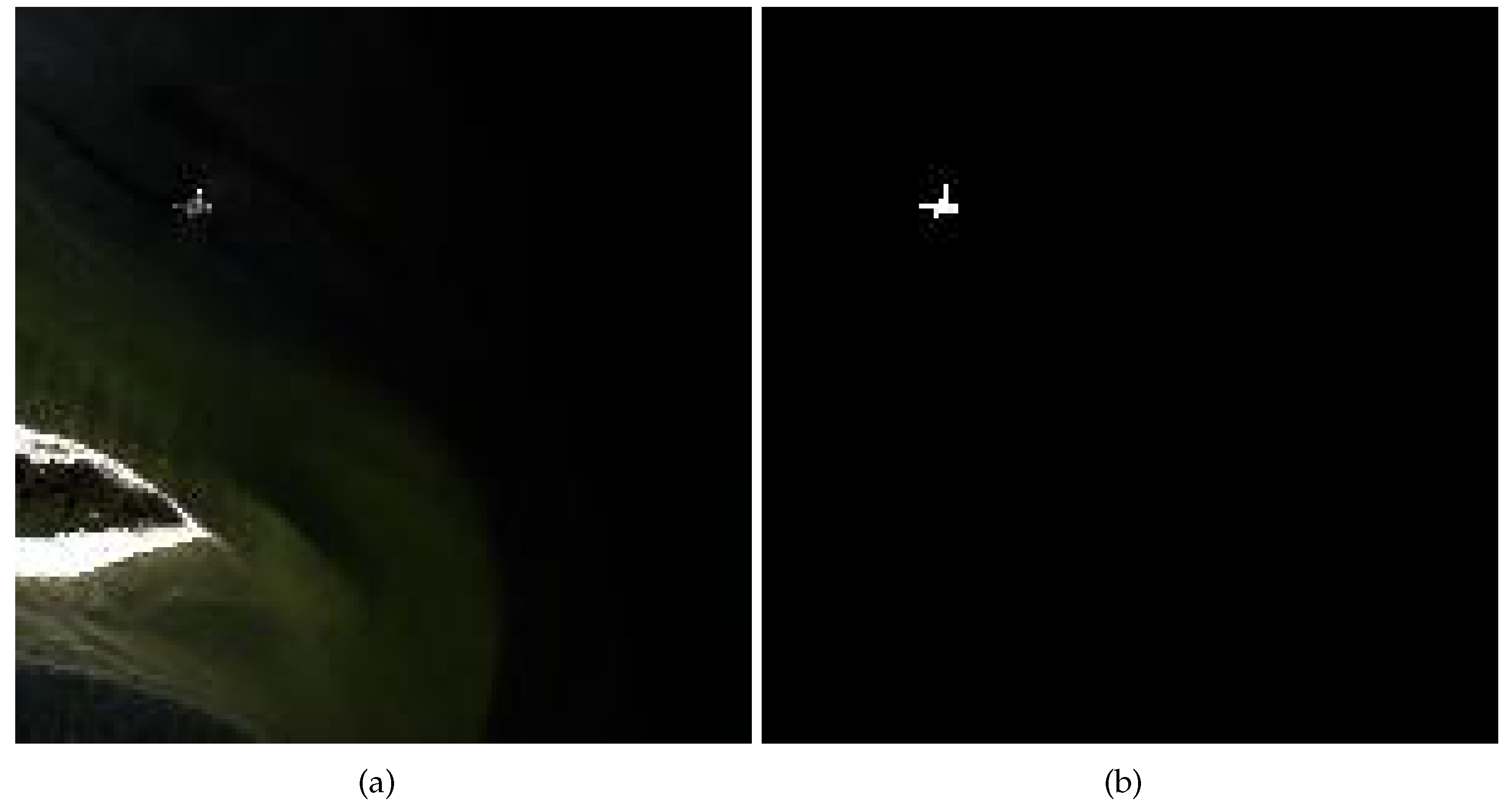
Figure 5.
Pavia city dataset. (a) RGB composite image. (b) Ground truth.
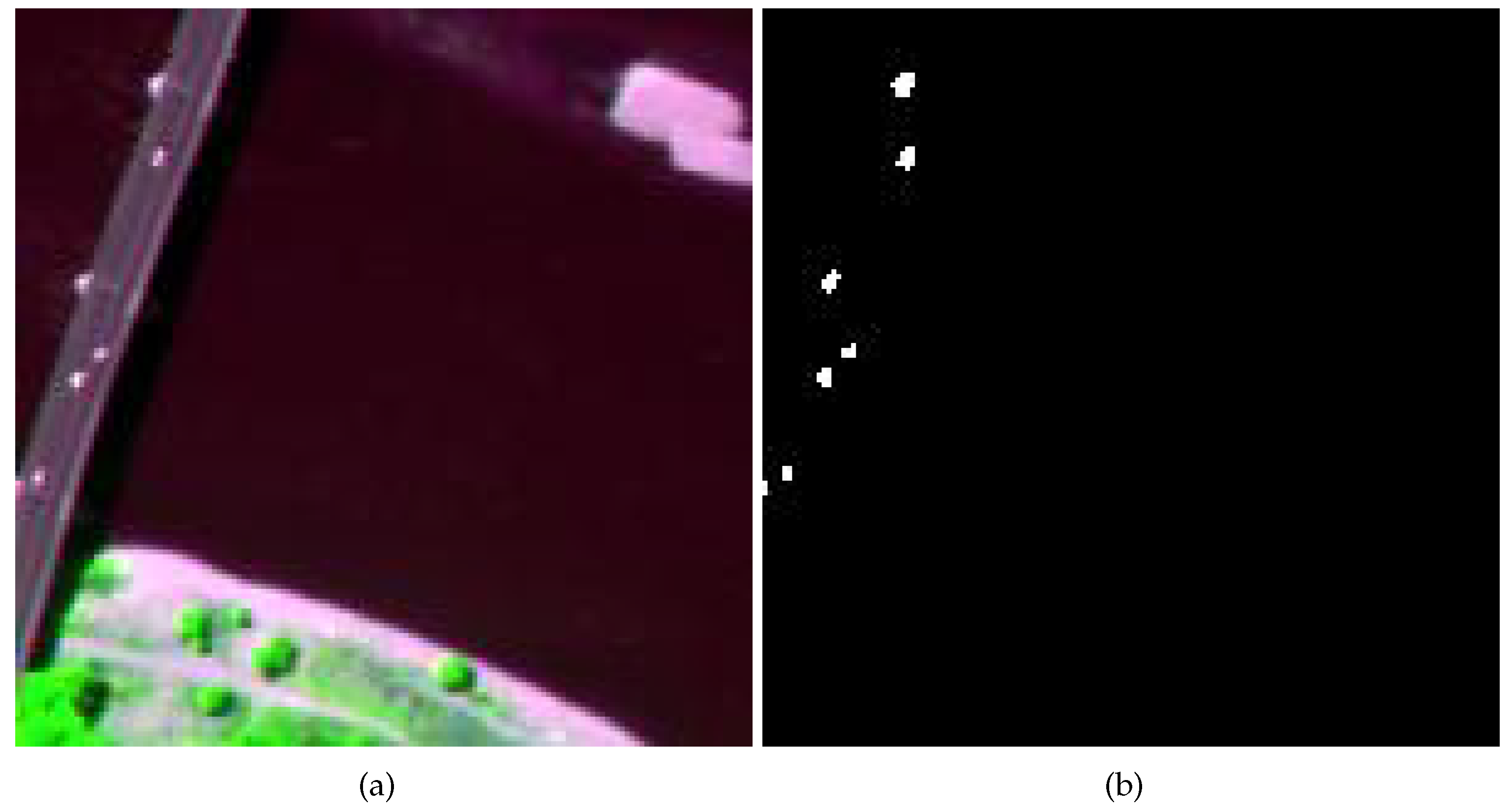
Figure 6.
San Diego-I dataset. (a) RGB composite image. (b) Ground truth.
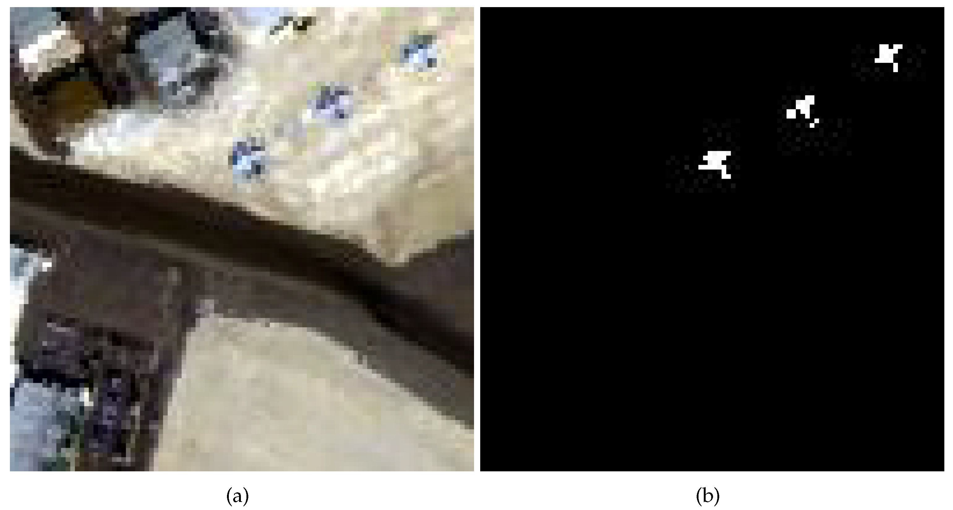
Figure 7.
San Diego-II dataset. (a) RGB composite image. (b) Ground truth.
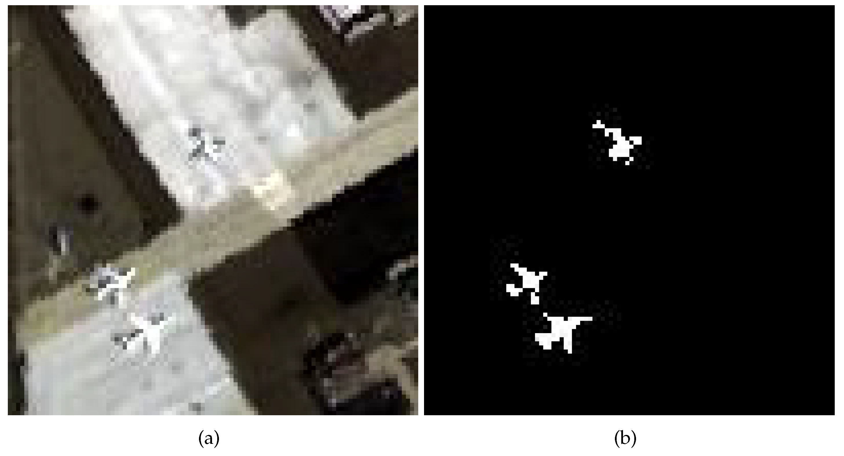
Figure 8.
Gulfport dataset. (a) RGB composite image. (b) Ground truth.
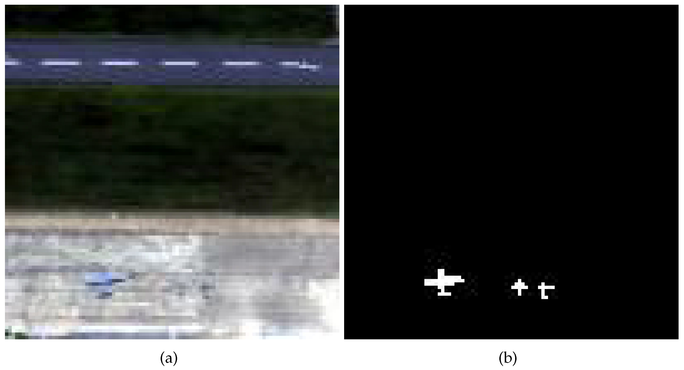
Figure 9.
Detection maps of all approaches on Beach dataset. (a) RX. (b) CRD. (c) AED. (d) KIFD. (e) PTA. (f) RGAE. (g) SSIIF. (h) Ours.
Figure 9.
Detection maps of all approaches on Beach dataset. (a) RX. (b) CRD. (c) AED. (d) KIFD. (e) PTA. (f) RGAE. (g) SSIIF. (h) Ours.
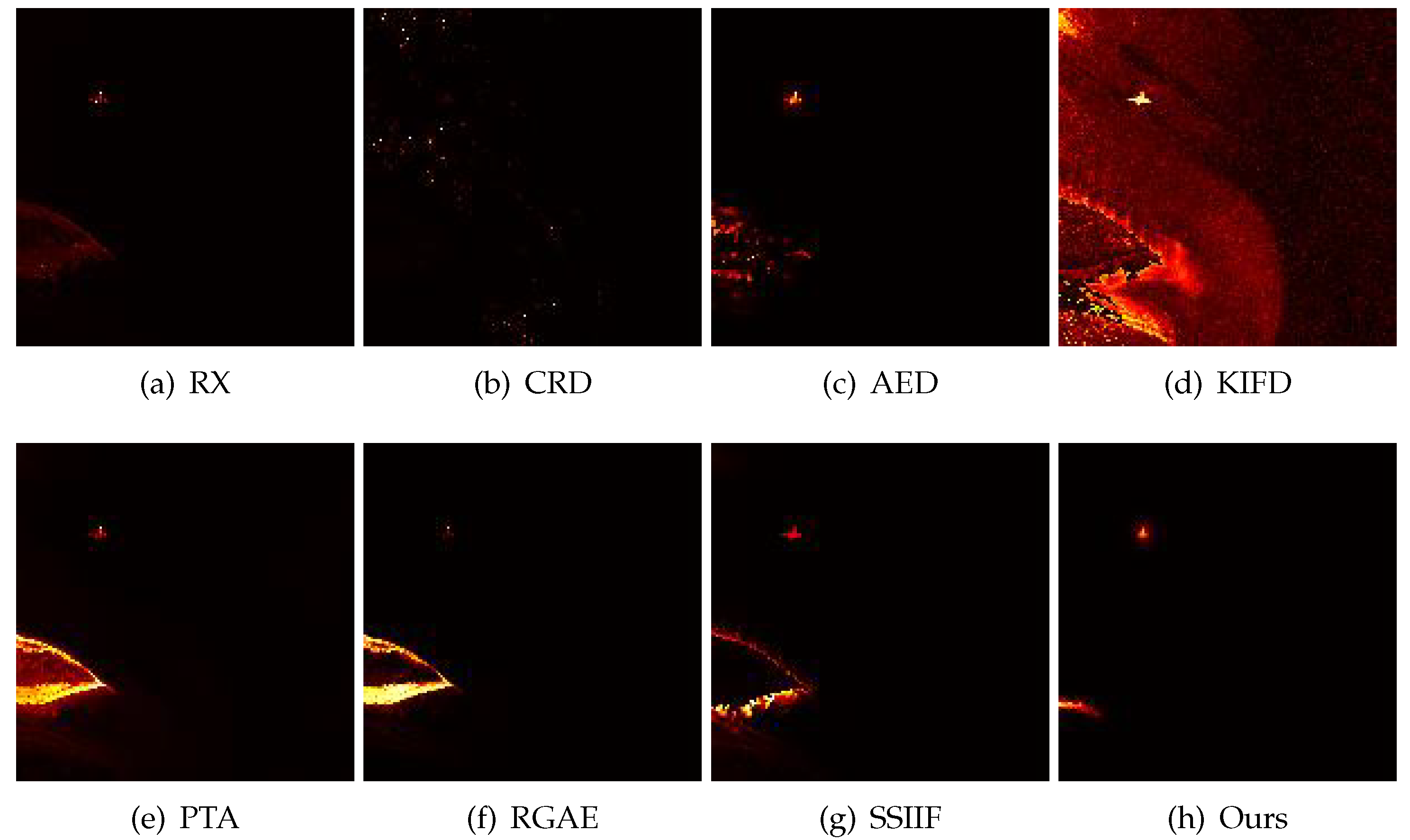
Figure 10.
Detection maps of all approaches on Pavia city dataset. (a) RX. (b) CRD. (c) AED. (d) KIFD. (e) PTA. (f) RGAE. (g) SSIIF. (h) Ours.
Figure 10.
Detection maps of all approaches on Pavia city dataset. (a) RX. (b) CRD. (c) AED. (d) KIFD. (e) PTA. (f) RGAE. (g) SSIIF. (h) Ours.
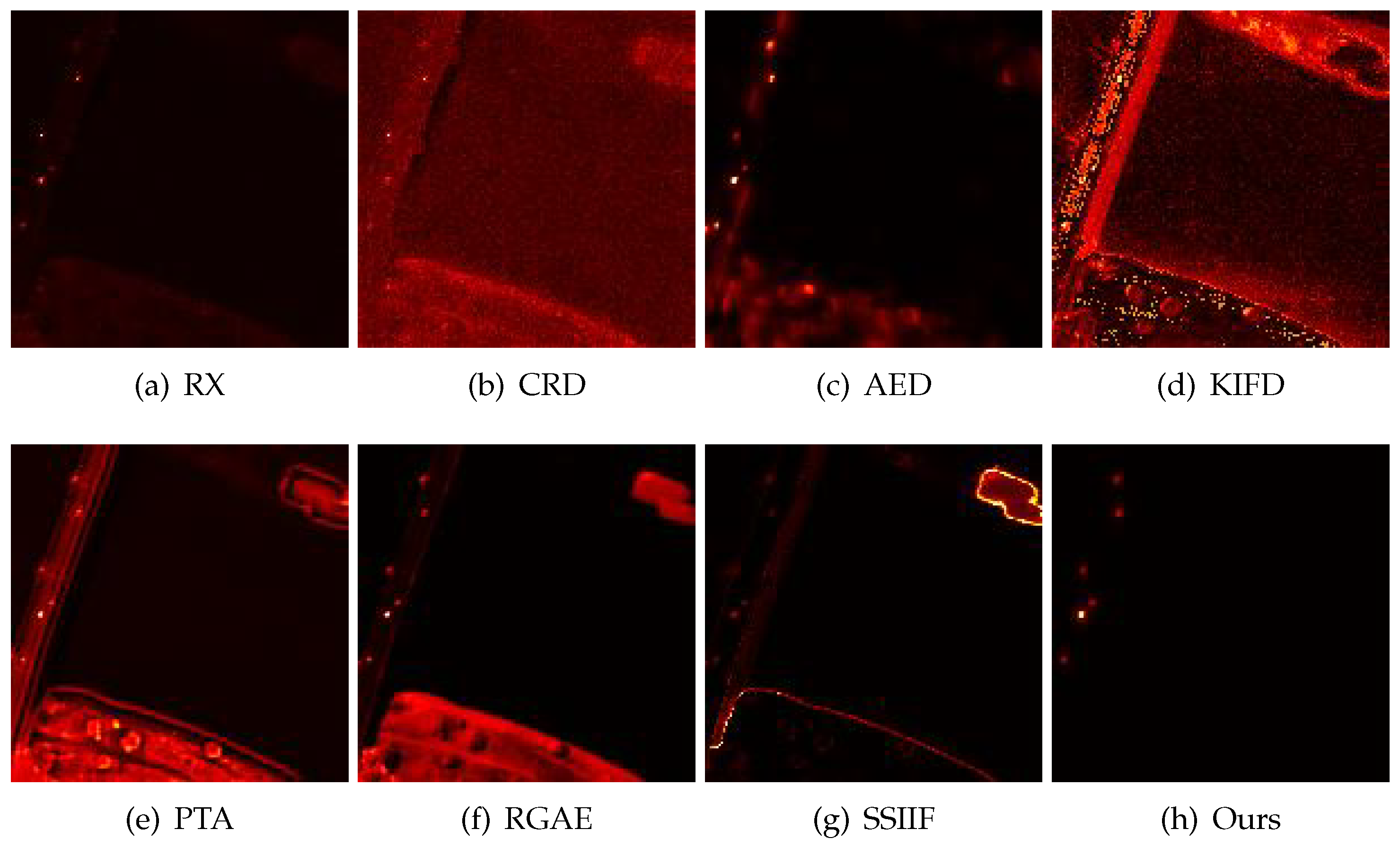
Figure 11.
Detection maps of all approaches on San Diego-I dataset. (a) RX. (b) CRD. (c) AED. (d) KIFD. (e) PTA. (f) RGAE. (g) SSIIF. (h) Ours.
Figure 11.
Detection maps of all approaches on San Diego-I dataset. (a) RX. (b) CRD. (c) AED. (d) KIFD. (e) PTA. (f) RGAE. (g) SSIIF. (h) Ours.
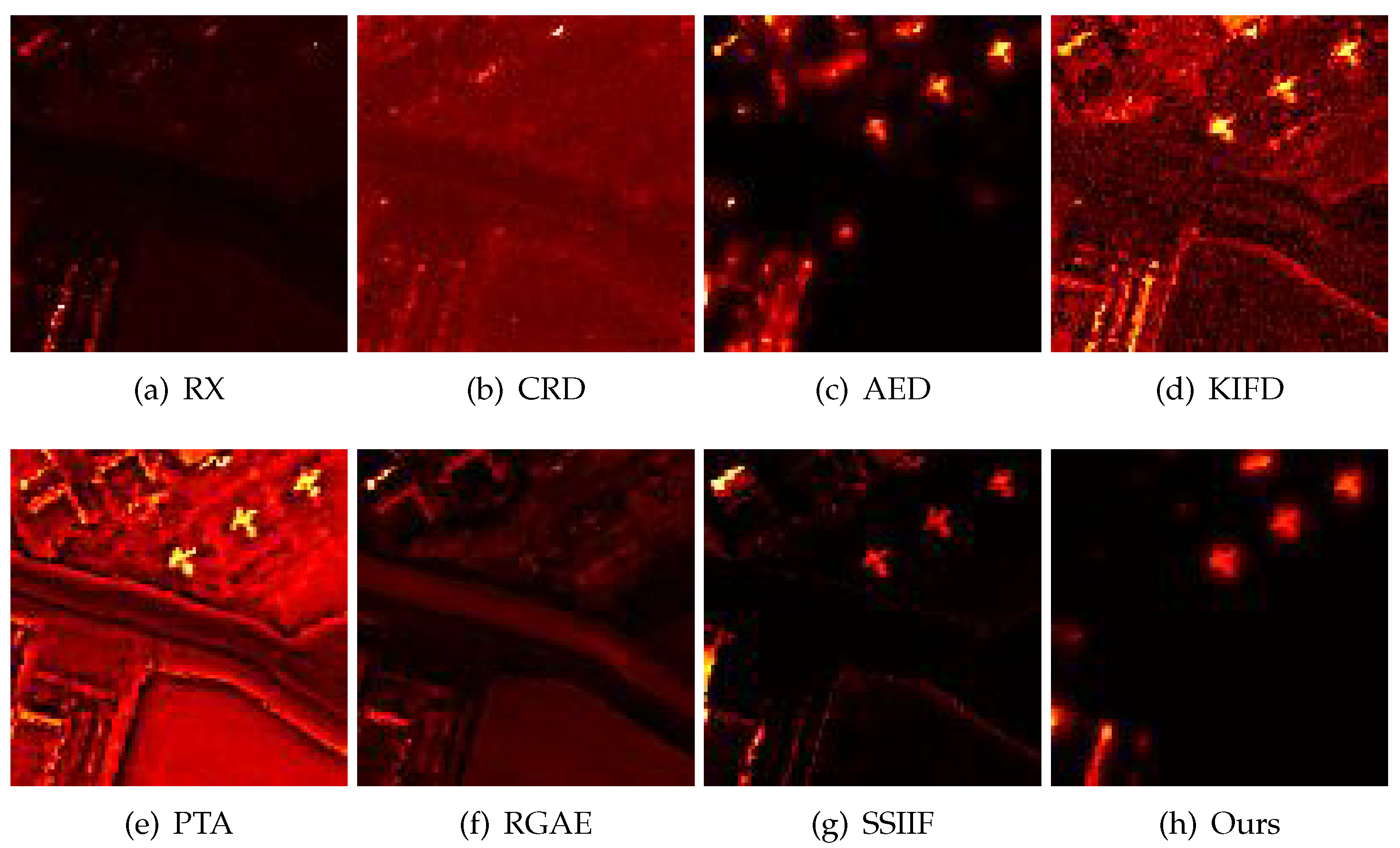
Figure 12.
Detection maps of all approaches on San Diego-II dataset. (a) RX. (b) CRD. (c) AED. (d) KIFD. (e) PTA. (f) RGAE. (g) SSIIF. (h) Ours.
Figure 12.
Detection maps of all approaches on San Diego-II dataset. (a) RX. (b) CRD. (c) AED. (d) KIFD. (e) PTA. (f) RGAE. (g) SSIIF. (h) Ours.
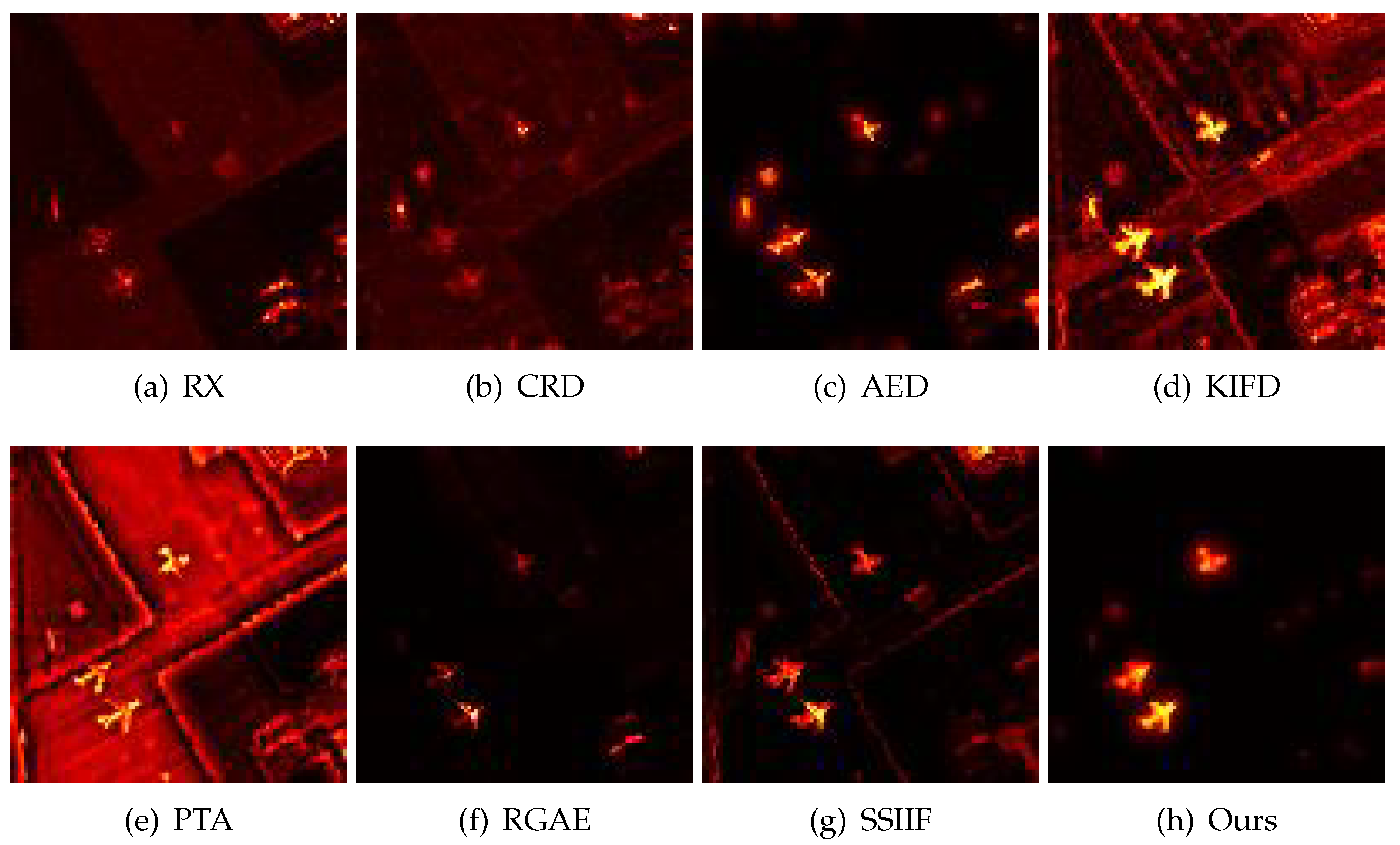
Figure 13.
Detection maps of all approaches on Gulfport dataset. (a) RX. (b) CRD. (c) AED. (d) KIFD. (e) PTA. (f) RGAE. (g) SSIIF. (h) Ours.
Figure 13.
Detection maps of all approaches on Gulfport dataset. (a) RX. (b) CRD. (c) AED. (d) KIFD. (e) PTA. (f) RGAE. (g) SSIIF. (h) Ours.
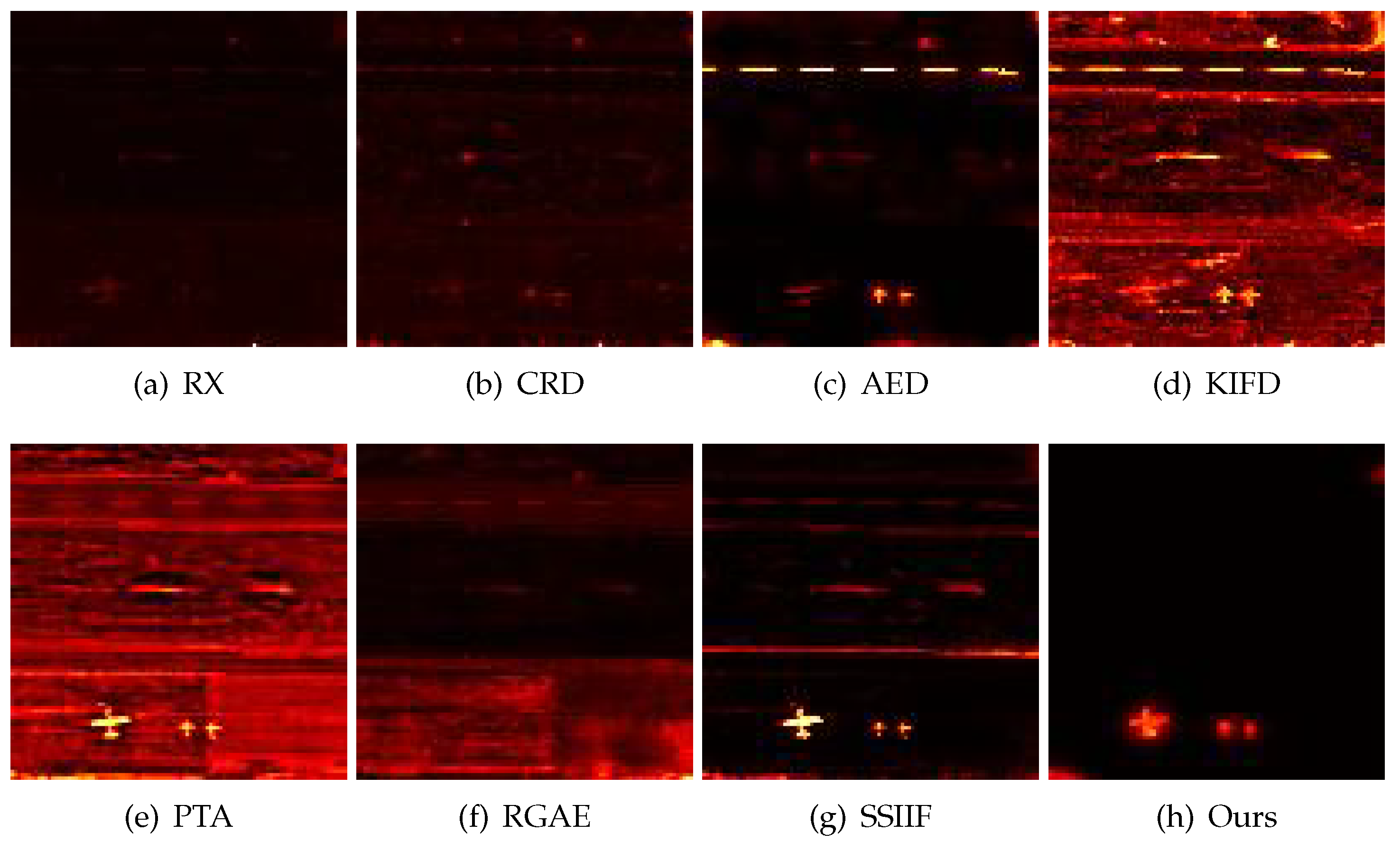
Figure 14.
ROC curves of all detection techniques on all datasets. (a) Beach dataset, (b) Pavia city dataset. (c) SanDiego-I dataset. (d) SanDiego-II dataset. (e) Gulfport dataset.
Figure 14.
ROC curves of all detection techniques on all datasets. (a) Beach dataset, (b) Pavia city dataset. (c) SanDiego-I dataset. (d) SanDiego-II dataset. (e) Gulfport dataset.
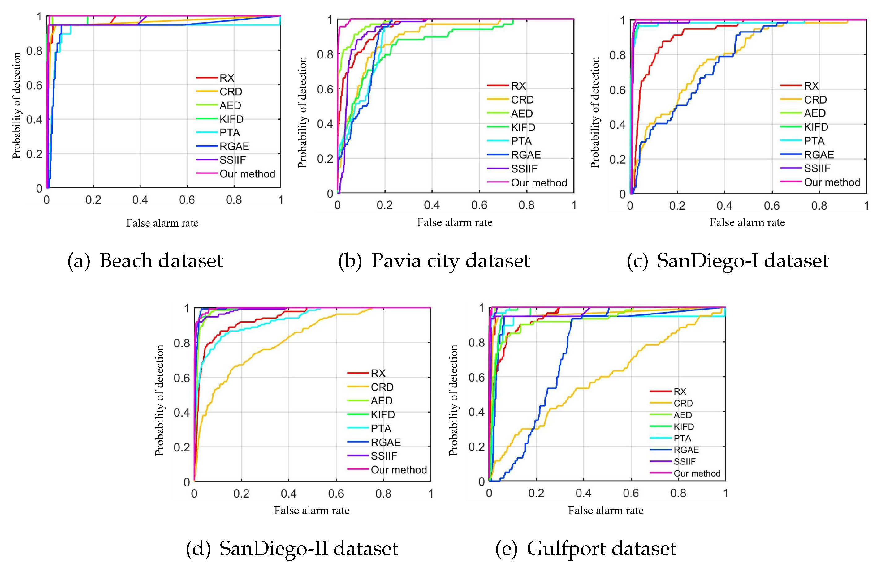
Figure 15.
The influence of different parameters in the spectral anomaly detection branch. (a) Different numbers of isolation trees q. (b) Different numbers of superpixels N.
Figure 15.
The influence of different parameters in the spectral anomaly detection branch. (a) Different numbers of isolation trees q. (b) Different numbers of superpixels N.
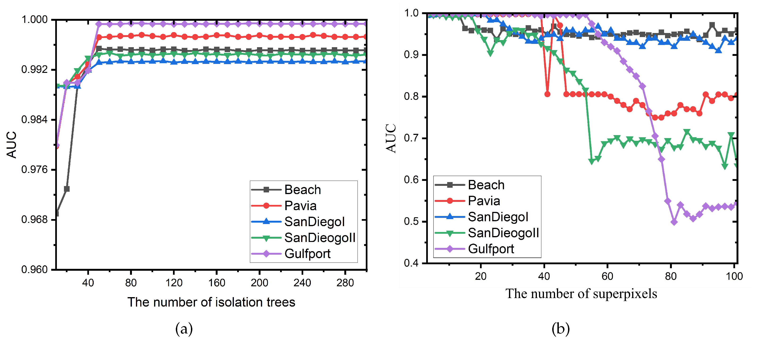
Figure 16.
The influence of different sizes of window in the spatial anomaly detection branch.
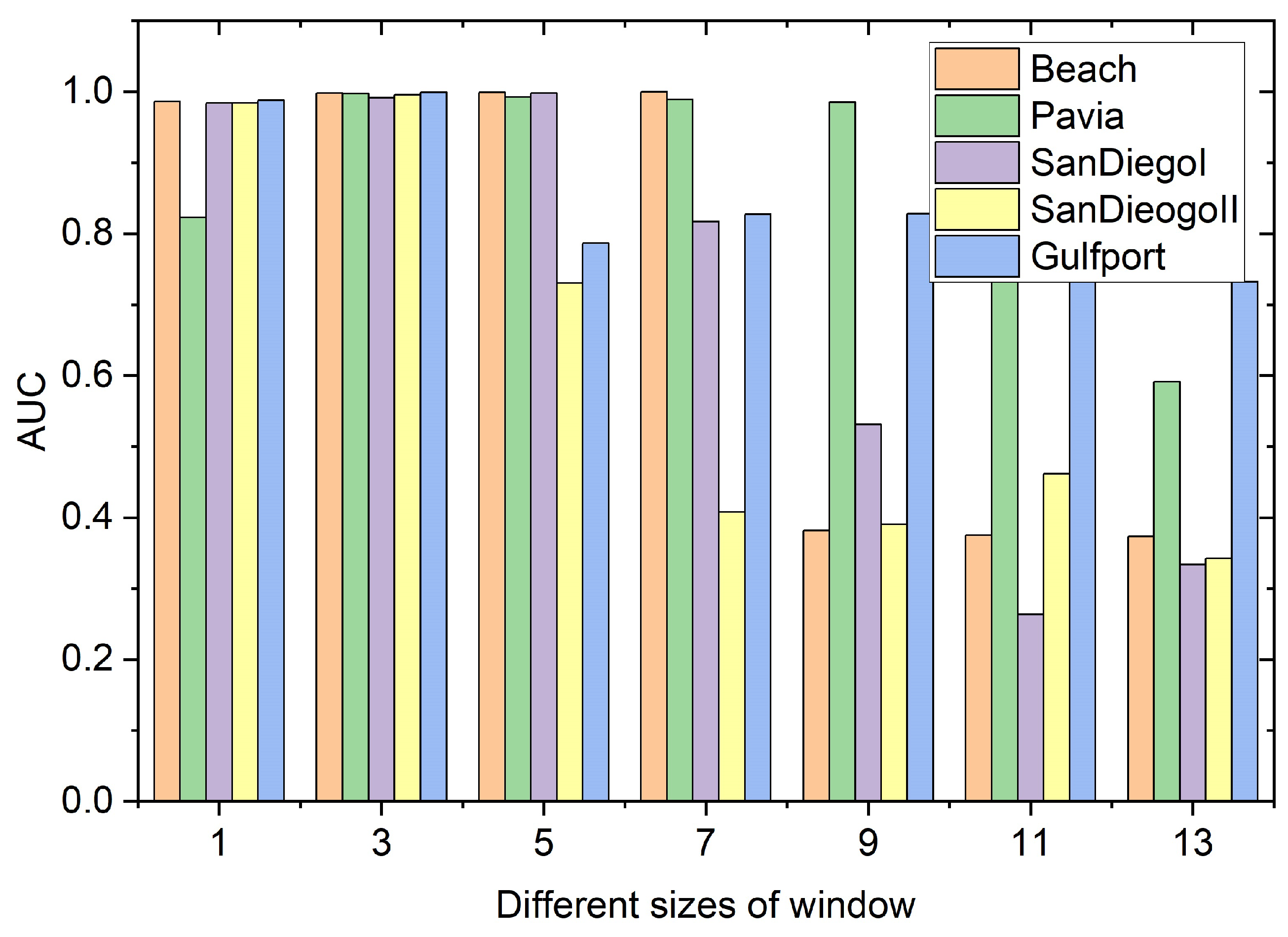

Table 1.
Detection results of all studied approaches. The best effect is displayed in bold.
| Datasets | RX | CRD | AED | KIFD | PTA | RGAE | SSIIF | Ours |
| Beach | 0.9807 | 0.9727 | 0.9974 | 0.9905 | 0.9184 | 0.9393 | 0.9672 | 0.9978 |
| Pavia | 0.9538 | 0.8941 | 0.9793 | 0.8742 | 0.9061 | 0.9042 | 0.9345 | 0.9972 |
| SanDiegoI | 0.9219 | 0.7826 | 0.9915 | 0.9934 | 0.9791 | 0.7914 | 0.9775 | 0.9949 |
| SanDiegoII | 0.9403 | 0.9687 | 0.9846 | 0.9931 | 0.9292 | 0.9929 | 0.9811 | 0.9956 |
| Gulfport | 0.9526 | 0.9618 | 0.9314 | 0.9683 | 0.9955 | 0.7583 | 0.9971 | 0.9990 |
Table 2.
The detection effect of different components in the proposed framework.
| Datasets | Beach | Pavia | SanDiegoI | SanDiegoII | Gulfport |
| Spatial branch | 0.9866 | 0.9889 | 0.9844 | 0.9872 | 0.9967 |
| Spectral branch | 0.9790 | 0.9332 | 0.9833 | 0.9824 | 0.9918 |
| Ours | 0.9978 | 0.9972 | 0.9949 | 0.9956 | 0.9990 |
Table 3.
Running time of different detection approaches.
| Datasets | RX | CRD | AED | KIFD | PTA | RGAE | SSIIF | Ours |
| Beach | 0.24 | 280.39 | 28.04 | 52.08 | 51.74 | 311.74 | 47.41 | 36.18 |
| Pavia | 0.13 | 274.38 | 31.64 | 61.41 | 31.09 | 181.79 | 33.64 | 31.73 |
| SanDiegoI | 0.13 | 136.45 | 21.93 | 37.41 | 24.08 | 125.17 | 30.41 | 25.15 |
| SanDiegoII | 0.11 | 142.62 | 19.92 | 32.73 | 24.33 | 147.51 | 28.33 | 24.51 |
| Gulfport | 0.12 | 119.01 | 21.65 | 37.31 | 24.57 | 140.86 | 29.73 | 28.26 |
Disclaimer/Publisher’s Note: The statements, opinions and data contained in all publications are solely those of the individual author(s) and contributor(s) and not of MDPI and/or the editor(s). MDPI and/or the editor(s) disclaim responsibility for any injury to people or property resulting from any ideas, methods, instructions or products referred to in the content. |
© 2024 by the authors. Licensee MDPI, Basel, Switzerland. This article is an open access article distributed under the terms and conditions of the Creative Commons Attribution (CC BY) license (http://creativecommons.org/licenses/by/4.0/).
Copyright: This open access article is published under a Creative Commons CC BY 4.0 license, which permit the free download, distribution, and reuse, provided that the author and preprint are cited in any reuse.


