Submitted:
11 December 2025
Posted:
14 December 2025
You are already at the latest version
Abstract
This study explores the spatial relationship between frequent physical distress (FPD) and socioeconomic as well as health-related factors across the contiguous United States. FPD, defined as having 14 or more physically unhealthy days within the past month, serves as an important measure of overall population health. While many studies have examined the causes of mental distress, research on the geographic variation and social context of physical distress remains limited. Using data from 2,673 U.S. counties, we analyzed how socioeconomic conditions and health indicators relate to FPD at both national and local levels. Ordinary Least Squares (OLS) multivariate regression model was first used to assess general associations, followed by Geographically Weighted Regression (GWR) and Multiscale Geographically Weighted Regression (MGWR) to identify spatially varying and scale-dependent relationships. Comparing the GWR and MGWR results revealed that several predictors of FPD operate at different spatial scales, reflecting local heterogeneity in health outcomes. Counties in the southeastern United States, particularly those with higher levels of socioeconomic disadvantage and poorer health conditions, showed elevated FPD rates. These findings highlight the importance of accounting for spatial context when addressing physical distress and suggest that locally tailored public health strategies may be more effective than uniform national approaches.
Keywords:
Frequent Physical Distress (FPD)
; socioeconomic and health-related factors
; Geographical Weighted Regression (GWR)
; Multiscale Geographically Weighted Regression (MGWR
1. Introduction
A major indicator of population health burden in the U.S. is the prevalence of frequent physical distress (FPD) which is generally defined as adults who report 14 or more physically unhealthy days in the preceding 30 days [1]. Analyses conducted at the county level reveal distinct regional variations in FPD. For instance, one study found that between 1995 and 2012 the prevalence of frequent physical distress rose nationally from about 10. 1 percent to 12. 3 percent with the highest rates occurring in counties in parts of southern Alabama, eastern Kentucky, western West Virginia, and the Texas-Mexico borderlands [2]. Moreover, data at the national level reveals significant state-by-state variation with West Virginia and Kentucky reporting FPD prevalence significantly higher than the U.S. average (~12%) [3]. While a lot of research has concentrated on specific behavioral risk factors (like obesity, smoking and physical inactivity), more attention is being paid to how larger socioeconomic and health-related contextual factors influence physical distress and how these relationships differ spatially.
FPD is likely to be influenced by socioeconomic and health-related factors in a variety of ways. The risk of FPD may be increased by low socioeconomic status (SES) which includes lower income, lower educational attainment restricted access to healthcare a higher prevalence of chronic diseases and unhealthy behaviors like smoking or physical inactivity that tend to cluster in underprivileged communities [4,5]. Furthermore, geographic differences in the prevalence of FPD indicate that spatial context is important: frequent physical distress has been linked to living in a county with higher rates of obesity, smoking or lack of insurance [2,6]. For example, states in the U.S. Southeast report FPD prevalences among older adults that are more than twice the rate of highest-education and high-income populations. However, a lot of current analyses rely on global regression techniques and national or regional aggregates which assume that the relationships between FPD and its determinants are consistent throughout space. Critical local variations and the multiscale nature of health-geographic processes may be obscured by such an assumption.
Furthermore, statistical analysis needs to consider a common methodological problem found in literature. Health data seldom satisfies the assumption that relationships between variables are constant throughout a study area which is a prerequisite for traditional global regression techniques like Ordinary Least Square (OLS). Disease prevalence, access to care, and environmental exposures are examples of health indicators that often show spatial heterogeneity or location-specific variations. Because it is becoming more widely acknowledged that health outcomes frequently exhibit spatial heterogeneity, spatial regression analysis has become increasingly popular in health research. To address this problem, Geographically Weighted Regression (GWR) was created which allows regression coefficients to change over space. This allows for a more nuanced analysis that can capture regional variations in health-related relationships [7,8,9]. GWR is especially helpful for understanding localized risk factors and locating disease hotspots or spatial clusters [10,11,12,13].
However, standard GWR has the drawback of treating all explanatory variables as functioning at the same spatial scale even though some determinants may act at larger spatial scales (region/state) and others at finer ones (neighborhood/county). By allowing each predictor to have its own spatial bandwidth, the more recent multiscale geographically weighted regression (MGWR) recognizes that determinants may operate at different scales and provides deeper understanding of both local and multiscale processes (e.g., when a socioeconomic factor affects FPD at a larger regional scale while a health-behavior variable affects it at a local neighborhood scale) [14,15].
In this study, we employ both GWR and MGWR to investigate the spatial relationship between FPD and a wide range of socioeconomic and health-related factors in 2,673 contiguous U.S. counties. Our three objectives are: (1) to evaluate the global (overall) associations between FPD and explanatory variables (2) to find local and multiscale variation in those associations and (3) to compare GWR and MGWR results to determine whether MGWR offers better explanatory power and deeper interpretive insight. To create geographically targeted public health interventions and policies that are suited to local context, scale and need, we aim to identify spatially explicit patterns of FPD determinants.
2. Materials and Methods
2.1. Frequent Physical Distress (FPD)
The percentage of adults who report having poor physical health for 14 or more days in the previous 30 days is known as Frequent Physical Distress (FPD) which is a recognized indicator of physical health burden. The Behavioral Risk Factor Surveillance System (BRFSS), a state-based nationally representative health survey run yearly by the Centers for Disease Control and Prevention (CDC) is the source of FPD. Responses to the question “Now thinking about your physical health which includes physical illness and injury for how many days during the past 30 days was your physical health not good?” are used to calculate the prevalence of FPD among the adult population in U.S. and serve as a proxy for the population-level burden of chronic disease, injury, and functional limitations [16,17]. We used age-adjusted FPD data for contiguous U.S. counties in 2023 as shown in Figure 1.
2.2. Socioeconomic and Health-Related Factors
According to Ha (2025), we included a number of socioeconomic and health-related factors to improve the analysis robustness. These factors includes: (1) health behavior factors (percentage of adult smoking, percentage of adult obesity, food environment index, percentage of physical activity, percentage of population with access to exercise opportunities, percentage of excessive drinking, and percentage of adults with insufficient sleep), (2) clinical care factors (percentage of population without health insurance, ratio of primary care physicians, ratio of mental health providers, preventable hospital stays), (3) social and economic factors: (percentage of adults with college degree, percentage of population over age 16 unemployed, the number of membership organizations per 10,000 residents, median household income), (4) demographic factors (percentage of population ages 65 and over, percentage of black population, percentage of female population, percentage of population living in rural areas) [17]. Data for these socioeconomic and health-related factors were obtained from a range of external datasets because the SMART BRFSS did not include many variables related to physical health [18,19].
For the source of the data, the BRFSS provided information on health behaviors such as the proportion of adult smokers, obesity rates, and excessive drinking. The American Medical Association (AMA) and the Small Area Health Insurance Estimates (SAHIE) provided clinical care data such as the ratio of uninsured adults and primary care physicians. In addition, CMS, National Provider Identification and Mapping Medicare Disparities Tool provided information on mental health providers and preventable hospital stays respectively. Moreover, the American Community Survey (ACS) provided data on the proportion of people with college degrees, and Bureau of Labor Statistics provided information on unemployment. Also, County Business Patterns provided data on social associations. Lastly, Census Population Estimates were used to determine demographic variables like the proportion of adults 65 and older. the proportion of African Americans. the proportion of females. and the proportion of rural residents [13,18,19]. To be consistent with the time frame of the SMART BRFSS and frequent physical distress (FPD) data, most of these variables from various database sources used Census Population Estimates in 2021 and ACS 5-year estimates from 2017–2021.
2.3. Statistical Analysis
This study investigated the geographic relationship between frequent physical distress (FPD) and socioeconomic and health-related factors using a three-step method. The data didn’t need to be transformed according to an initial analysis of data skewness. Next, a set of explanatory variables was used to find significant predictors using a stepwise ordinary least square (OLS) regression. Moreover, multicollinearity in our predictors was evaluated using the variance inflation factor (VIF) [20]. Finally, both Geographically Weighted Regression (GWR) and Multiscale Geographically Weighted Regression (MGWR) models were developed to examine local variations and to provide deeper understanding of both local and multiscale processes in the relationship between FPD and socioeconomic and health-related factors using the identified most significant predictors.
An expansion of Geographically Weighted Regression (GWR), Multiscale Geographically Weighted Regression (MGWR), allows each predictor to vary spatially at its own optimum scale of geography. MGWR breaks the assumption of GWR of having all relationships operating at a single, constant bandwidth in the study area, by estimating a unique bandwidth for each predictor. This approach acknowledges the possibility that different covariates operate and influence the outcome at different spatial scales. For instance, regional socioeconomic indicators may differ more widely while environmental exposures or neighborhood features may differ more locally. As a result, MGWR offers a more adaptable and practical framework for simulating spatial heterogeneity.
The general formulation of MGWR can be written as:
where are the spatial coordinates for location , represents the intercept at the location i with coordinates of , denotes the location-specific coefficient for predictor estimated with its own bandwidth , and is the error term. The bandwidth controls the degree of spatial smoothing for each variable and is selected through model optimization procedures such as the corrected Akaike Information Criterion (AICc). By estimating variable-specific bandwidths, MGWR identifies which processes are global (large bandwidth), regional (moderate bandwidth), or local (small bandwidth), providing deeper insights into the spatial structure of relationships [14,15].
MGWR produces better interpretability, better model fit, and a more accurate depiction of multiscale spatial processes than GWR. A single bandwidth is used for all predictors in standard GWR assuming that each variable has an equal impact across the same geographic area [21]. When various determinants function at essentially different scales this can result in either oversmoothing or undersmoothing. To overcome this constraint, MGWR permits flexible bandwidths that adapt to the spatial footprint of each variable resulting in parameter surfaces that more accurately represent theoretical predictions and empirical realities [14,15]. As a result, MGWR has become a widely used tool in environmental health, epidemiology, social sciences, and urban analytics for disentangling complex spatial relationships.
3. Results
3.1. Descriptive and Bivariate Statistics
The mean, standard deviations (SD), and bivariate statistics of both dependent and independent variables are shown in Table 1. For dependent variable, average frequent physical distress (FPD) in 2673 contiguous counties was 10.942 percent with a SD of 2.083. For health behavior factors, on average 19.983 percent of a county’s adult participants, were smokers with a SD of 4.004 percent. Moreover, on average 36.187 percent and 34.591 percent of adult participants in the counties had obesity and insufficient sleep respectively with a SD of 4.674 percent and 3.591 percent. Additionally, average of food environment index was 7.502 with a SD of 1.058, while the percentage of physically inactive, the percentage of adequate access to physical activity, and the percentage of alcohol impaired were on average 25.627 percent, 63.732 percent, and 19.034 percent with a SD of 5.088 percent, 21.258 percent, and 3.174 percent respectively. For clinical factors, on average, the percentage of uninsured and the number of primary care physicians per 100,000 participants were 11.511 percent and 55.215 physicians with a SD of 5.029 percent and 34.401 physicians respectively. Furthermore, on average, mental health provider rate and preventable hospitalization rate were 191.972 and 3015.104 with a SD of 192.908 and 1112.770 respectively.
For socioeconomic factors, the percentage of adults with a college education and the percentage of unemployed adults, on average, were 58.984 percent and 4.710 percent with a SD of 11.296 percent and 1.655 percent respectively. Also, average number of membership associations per 10,000 population was 11.453 memberships with a SD of 4.684, and average median household income was 59,606.975 with a SD of 15,553.751. In terms of demographics, the average percent of a county’s population that was 65 years of age or older was 19.716 percent with a SD of 4.554 percent, while the African American population, on average, accounted for 9.574 percent of a county’s population with a SD of 14.282 percent. Moreover, on average, the percentage of female and the percentage of rural area were 49.782 percent and 53,376 percent respectively with a SD of 1.975 percent and 29.675 percent. The differences in these independent variables show that frequent mental distress (FPD) occurred in counties with heterogeneous behavioral, clinical, socioeconomic, and demographic characteristics [18].
3.2. OLS Regression Analyses
Table 2 summarizes the results from the OLS regression model. Two explanatory variables, namely the percentage of adult smoking and the percentage of physically inactive were excluded in the model due to the high VIF (VIF >5) and include 17 explanatory variables in the final model. An adjusted R2 value of 0.855 indicates that these 17 explanatory variables explained 85.5% of the total variance in the county-level frequent physical distress (FPD). The VIF was less than 4 for all explanatory variables, indicating no multicollinearity in the final OLS model. The FPD was significantly (p < 0.005) associated with 16 of the explanatory variables except the percentage with access to exercise. In health behavior variables, both the percentage of adult obesity and the percentage of insufficient sleep exhibit a strong positive relationship with FPD, while food environment index and the percentage of alcohol impaired show a significantly negative relationship with FPD.
In clinical care variables, all 4 variables namely, the percentage of uninsured, primary care physician (PCP) rate, mental health provider (MHP) rate, and preventable hospitalization rate all show a significant positive association with FPD. Among social economic environmental variables, a negative association to FPD was found with the percentage of college education, association rate, and median household income, while a positive association to FPD was discovered with the percentage of unemployment. Demographic variables also play a crucial role; the percentage of population ages 65 and older, the percentage of African American, and the percentage of female show significantly negative relationships with FPD, whereas the proportion of rural residents exhibits a significantly positive relationship with FPD. Overall, the results from the OLS analysis reveal that frequent physical distress (FPD) is influenced by a multifaceted set of explanatory variables, including health behaviors, clinical care, socioeconomic status, and demographic characteristics.
3.3. GWR and MGWR Analyses
Table 3 presents the numerical findings from both Geographically Weighted Regression (GWR) and the Multiscale Geographically Weighted Regression (MGWR) analysis examining frequent physical distress (FPD) in relation to selected explanatory variables. This table allows the parameter estimates and model performance produced by the OLS to be directly compared with the range of results generated by GWR and MGWR. Based on the results of the OLS’s statistically significant test, six most significant explanatory variables identified from physical health literature review were retained in both GWR and MGWR models. As shown in the table, the MGWR model demonstrated an average R2 value of 0.918 with a range between 0.492 and 0.958. This is significant improvement over both OLS and GWR models, which left approximately 15% and 9% of the variance in FPD unexplained respectively. In addition, the Akaike Information Criterion (AIC) value provides an estimate of model fit while penalizing complexity, and MGWR model clearly shows lower AIC value (1,671.088 vs. 1,633.507) than GWR model indicating a better-fitting model when comparing multiple models [18]. In the table, we also report the optimal number of neighbors and the proportion of features with significant results for each explanatory variable for the MGWR model.
Figure 2 illustrates the spatial distribution of the parameter estimates of the six selected explanatory variables. A negative association between the food environment index and frequent physical distress (FPD) were found in the most of counties in U.S. except some of counties in Oregon, Colorado, Ohio, Pennsylvania, and Florida (Figure 2a). For insufficient sleep, stronger positive relationships appeared primarily in portions of the southwest (Texas, New Mexico, Arizona, California, and Nevada), rocky mountain (Montana), and plains (North Dakota, South Dakota, and Nebraska) (Figure 2b). For the percentage of college education, negative associations were observed in the most of U.S. counties, especially, strong association within states of Kansas, Missouri, Oklahoma, and California (Figure 2c).
For the association rate, negative relationships were found in the most of U.S. counties, but positive relationships were discovered in some of western regions (California, Nevada, and Utah), rocky mountain (Montana), plains (South Dakota, Minnesota, and Iowa), southeast regions (Georgia, Florida, and Mississippi), and mid-east regions (New York) (Figure 2d). Regarding the median household income, stronger negative associations with FPD were found in parts of the southeast areas, especially, Louisiana, Arkansas, Missouri, Georgia, Florida, South Carolina, West Virginia, as well as great lakes regions such as Ohio and Michigan (Figure 2e). For the percentage of African American, stronger negative relationships were observed in portions of rocky mountain (Montana and Wyoming) and plain (North Dakota) regions, while stronger positive relationships were seen in parts of northwest regions (Washington, Oregon, and Idaho) (Figure 2f).
Level of significance of the coefficient also varied across the 48 contiguous U.S. states. Regarding food environment index, large portions of significant association with FPD (20.22% of significance) were found in parts of southwest (Texas, New Mexico, and Arizona) and Midwest regions (South Dakota, Wyoming, Minnesota, and Wisconsin) (Figure 3a). For the percentage of insufficient sleep, large parts of significant relationships with FPD (48.60% of significance) were observed in west (California, Nevada, Utah, and Montana), southwest (particularly, in portions of Arizona, New Mexico, and Texas), and southeast (Mississippi, Alabama, Tennessee, Kentucky, and West Virginia) regions (Figure 3b). For the percentage of college education and median household income, similar distribution of significance with FPD (60.40% and 61.83% of significance respectively) were observed, in majority of west and southeast states, including Washington, Oregon, Idaho, Mississippi, Alabama, Georgia, Florida, North Dakota, South Dakota, Louisiana, as well as parts of Midwest regions, including Minnesota, Michigan, Indiana, and Ohio (Figure 3c,e). Lastly, association rate and the percentage of African American also showed a similar significance distribution (8.79% and 10.73% of significance respectively), notably, in parts of rocky mountain (Montana and Wyoming), as well as portion of southwest (Texas) and southeast (West Virginia and Ohio) regions (Figure 3d,f).
4. Discussion
Frequent physical distress (FPD) exhibited pronounced spatial variation across U.S. counties in our analysis, with elevated rates concentrated in the Southeast and other areas characterized by socioeconomic disadvantage and poor health infrastructure. This geographic pattern echoes prior county-level findings that link population-level physical health burden to regional socioeconomic deprivation, chronic-disease prevalence, and constrained access to care and is consistent with patterns observed in similar county studies [2,22,23,24,25]. The national OLS model captured strong average associations—education, income, insurance coverage, preventable hospitalizations, obesity, and insufficient sleep were all meaningfully associated with higher FPD [26,27,28]. However, these global averages masked important local departures in both magnitude and sign. These empirical patterns in the study align with the geographic disparities described in earlier work and the maps and summary statistics presented in the study.
Our study employed Multiscale Geographically Weighted Regression (MGWR) to investigate the spatially varying relationships between frequent physical distress (FPD) and a comprehensive set of socioeconomic and health-related factors across the contiguous United States. The initial analysis clearly demonstrated that the global Ordinary Least Squares (OLS) model was less adequate, as evidenced by its lower goodness-of-fit and the statistically significant non-stationarity detected in the relationships. This finding underscores the necessity of employing local spatial models to accurately capture the geographically varying processes underlying FPD. Beyond what OLS and single-bandwidth GWR offer, MGWR adds two significant insights. First, we can empirically identify which determinants act locally (at the community/county level) and which act broadly (regional or supra-regional) by using MGWR which explicitly estimates a distinct spatial bandwidth for each covariate [29,30]. While clinical access and health and behavioral indicators displayed narrower bandwidths consistent with more localized effects socioeconomic measures (education income unemployment) generally returned larger bandwidths—indicating broad regional influence. Second, compared to both OLS and standard GWR MGWR produced coefficient surfaces that are less susceptible to oversmoothing or undersmoothing that can occur when a single bandwidth is applied to all predictors [14,15]. It also decreased overall AICc and increased adjusted R2. Because of these benefits MGWR is especially suitable for separating the multiscale processes that influence FPD [14,15].
Interpreting the multiscale patterns yields concrete substantive implications. The fact that socioeconomic indicators act at broader scales suggests that structural forces—labor markets, educational systems, regional health economies, and historical patterns of in-vestment—create a backdrop of vulnerability that elevates FPD across wide territories. In contrast, narrow spatial footprints for clinical access and behavioral factors imply that local health system capacity and community health behaviors can modify or amplify the underlying socioeconomic risks. Therefore, effective interventions must operate at multiple scales including county or community-level investments in primary care, preventive services and behavioral health programs as well as regional policies to address poverty, education, and insurance coverage [14,15,31].
Methodologically, our study illustrates best practices for spatial public-health re-search. Relying solely on OLS (global) model risk both ecological oversimplification and misleading inference because spatial non-stationarity and spatial dependence are pervasive in health outcomes. Although standard GWR handles non-stationarity, it assumes that all predictors have the same spatial scale which can mask mixed-scale processes and result in local collinearity in coefficient estimates [32]. By allowing covariate-specific bandwidths, MGWR corrects for this and produces parameter surfaces that more accurately represent theoretical predictions and empirical reality [14,15]. That said, MGWR is inherently exploratory and descriptive: while it improves local inference and identifies scale-specific patterns, causal claims still require temporally resolved, individual-level data and careful confounder control [14,32].
Critical geographic patterns were further highlighted by the MGWR coefficients spatial mapping. The southeast U.S. and the Appalachian regions consistently clustered the strongest positive coefficient values which indicate a more severe impact of the risk factors on frequent physical distress (FPD). A regional vulnerability zone where the population is most vulnerable to FPD appears to be created in these areas by the compounding effects of low socioeconomic status (SES) (education, income, and social association) and inadequate health behavior and infrastructure (insufficient sleep and food environment). For example, the Deep South has the greatest marginal impact of an increase in poverty on FPD and this finding is consistent with spatial disparities found for other chronic health issues [18,19]. This geographic pattern demonstrates that FPD is intricately linked to the historical economic, and environmental context of a location rather than being just an individual health outcome.
Finally, we acknowledge limitations that affect interpretation and future directions. First, county-level aggregation may obscure important within-county heterogeneity (ecological fallacy); finer-scale data (census tract or individual-level) would clarify neighborhood effects. Second, the cross-sectional design constrains causal inference—temporal or longitudinal MGWR/GTWR analyses would better separate exposure and outcome dynamics [14]. Third, the cross-sectional nature of the data limits causal inference and makes it impossible to evaluate temporal changes in FPD or its determinants even though MGWR outperforms global and single-scale spatial models. Furthermore, unobserved factors like local healthcare quality environmental exposures or community-level psychosocial stressors, may still skew the observed spatial associations even when a comprehensive set of socioeconomic and health-related variables is included. Lastly, some county estimates, particularly those derived from modeled BRFSS data for less-populated areas, may contain additional uncertainty that cannot be fully accounted for in the MGWR framework, potentially affecting the precision of local coefficient estimates.
5. Conclusions
This study demonstrates that frequent physical distress (FPD) in the United States is strongly spatially patterned and driven by a mixture of socioeconomic, clinical, behavior-al, and demographic factors that operate at different geographic scales. MGWR provided clearer, scale-sensitive insight than OLS or single-bandwidth GWR. That is, it identified which determinants were broad/regional and which were local, as well as improving model fit and reducing misleading smoothing of localized effects. These methodological benefits are translated into policy guidance- regional investments in socioeconomic conditions and insurance coverage should be complemented by county-level strengthening of primary care, targeted chronic-disease prevention, and community health promotion where local drivers are strongest [14,15].
In order to examine causal pathways, combine environmental and built-environment exposures at finer spatial resolution, and assess the effects of place-based policy initiatives, future research should focus on longitudinal and multilevel approaches. MGWR results can be incorporated into routine public health surveillance to better focus resources and, crucially, to support mixed-scale policies that address both local health system requirements and structural determinants. The most effective way to lessen geographic disparities in physical distress and enhance population health is to combine multiscale spatial analysis with focused treatments.
Funding
This research did not receive any specific grant from funding agencies in the public, commercial, or not-for-profit sectors.
Data Availability Statement
Data are contained within this article.
Acknowledgments
The author would like to thank the anonymous reviewers for their constructive comments and suggestions to improve the paper. The contents of this publication are solely the responsibility of the authors.
Conflicts of Interest
The author declares no conflicts of interest.
References
- Centers for Disease Control Prevention Frequent physical distress: Indicators measures from the Behavioral Risk Factor Surveillance System (BRFSS), U.S. Department of Health and Human Services. 2024. Available online: https://www.cdc.gov/brfss.
- Dwyer-Lindgren, L.; Mackenbach, J.P.; van Lenthe, F.J.; Mokdad, A.H. Self-reported general health, physical distress, mental distress, and activity limitation by US county, 1995–2012. Population Health Metrics 2017, 15, 16. [Google Scholar] [CrossRef]
- United Health Foundation. America’s Health Rankings Annual Report 2018. Available online: https://assets.americashealthrankings.org/app/uploads/ahrannual-2018.pdf.
- Hunyadi, J.V.; Zhang, K.; Xiao, Q.; Strong, L.L.; Bauer, C. Spatial and Temporal Patterns of Chronic Disease Burden in the U.S., 2018–2021. American Journal of Preventive Medicine 2025, 68(1), 107–115. [Google Scholar] [CrossRef]
- Zhao, H.; Yue, L.; Jia, Z.; Su, L. Spatial Inequalities and Influencing Factors of Self-Rated Health and Perceived Environmental Hazards in a Metropolis: A Case Study of Zhengzhou City, China. International Journal of Environmental Research and Public Health 2022, 19(12), 7551. [Google Scholar] [CrossRef]
- Jacobs, M.M.; Burch, A.E. Disparities in perceived physical and mental wellness: Relationships between social vulnerability, cardiovascular risk factor prevalence, and health behaviors among elderly US residents. Journal of Primary Care & Community Health 2023, 14, 21501319231163639. [Google Scholar] [CrossRef]
- Fotheringham, A.S.; Brunsdon, C.; Charlton, M. Geographically Weighted Regression: The Analysis of Spatially Varying Relationships; Wiley, 2002. [Google Scholar]
- Ha, H. Using geographically weighted regression for social inequality analysis: association between mentally unhealthy days (MUDs) and socioeconomic status (SES) in U.S. counties. Int. J. Environ. Health Res. 2018. [Google Scholar] [CrossRef] [PubMed]
- Sá, AC L.; Pereira, J.M.C.; Charlton, M.E.; Mota, B.; Barbosa, P.M.; Fotheringham, A.S. The pyrogeography of sub-Saharan Africa: A study of the spatial non-stationarity of fire–environment relationships using GWR. Journal of Geographical Systems 2011, 13(3), 227–248. [Google Scholar] [CrossRef]
- Chan, T.C.; Chiang, P.H.; Su, M.D.; Wang, H.W.; Liu, M.S. Geographic disparity in chronic obstructive pulmonary disease (COPD) mortality rates among the Taiwan population. PLoS ONE 2014, 9, e98170. [Google Scholar] [CrossRef]
- Lin, C.H.; Wen, T.H. Using geographically weighted regression (GWR) to explore spatial varying relationships of immature mosquitoes and human densities with the incidence of dengue. Int J Env Res Pub He 2011, 8, 2798–2815. [Google Scholar] [CrossRef]
- Ha, H.; Xu, Y. An ecological study on the spatially varying association between adult obesity rates and altitude in the United States: using geographically weighted regression. International Journal of Environmental Health Research 2020. [Google Scholar] [CrossRef]
- Ha, H. Identifying spatial association between Frequent Mental Distress (FMD) and air pollution (PM2.5): Evidence from 2,648 counties in the United States. Applied Spatial Analysis and Policy 2025. [Google Scholar] [CrossRef]
- Fotheringham, A.S.; Yang, W.; Kang, W. Multiscale Geographically Weighted Regression (MGWR). Annals of the American Association of Geographers 2017, 107(6), 1247–1265. [Google Scholar] [CrossRef]
- Oshan, T.M.; Li, Z.; Kang, W.; Wolf, L.J.; Fotheringham, A.S. mgwr: A Python Implementation of Multiscale Geographically Weighted Regression for Investigating Process Spatial Heterogeneity and Scale. ISPRS International Journal of Geo-Information 2019, 8(6), 269. [Google Scholar] [CrossRef]
- Centers for Disease Control Prevention Chronic Disease Indicators: Health Status—Indicator, D.e.f.i.n.i.t.i.o.n.s.; US Department of Health and Human Services. 2023. Available online: https://www.cdc.gov/cdi/indicator-definitions/health-status.html.
- County Health Rankings & Roadmaps. Frequent Physical Distress; University of Wisconsin Population Health Institute. 2023. Available online: https://www.countyhealthrankings.org.
- Ha, H. Geographic distribution of lung and bronchus cancer mortality and elevation in the United States: exploratory spatial data analysis and spatial statistics. ISPRS International Journal of Geo-Information. 2025. [Google Scholar] [CrossRef]
- Ha, H. Using geographically weighted regression for social inequality analysis: Association between Mentally Unhealthy Days (MUDs) and socioeconomic status (SES) in U.S. Counties. International Journal of Environmental Health Research 2018. [Google Scholar] [CrossRef] [PubMed]
- Rogerson, P.A. Statistical Methods for Geography, 2nd ed.; Sage: London, UK, 2006. [Google Scholar]
- Brunsdon, C.; Fotheringham, A.S.; Charlton, M. Geographically weighted regression—Modelling spatial non-stationarity. Journal of the Royal Statistical Society: Series D (The Statistician) 1998, 47(3), 431–443. [Google Scholar] [CrossRef]
- Centers for Disease Control Prevention (CDC) PLACES: Local data for better health—Measure definitions: Frequent physical, d.i.s.t.r.e.s.s.; US Department of Health and Human Services. 2024. Available online: https://www.cdc.gov/places/measure-definitions/health-status.html.
- University of Wisconsin Population Health Institute; Robert Wood Johnson Foundation. County Health Rankings & Roadmaps 2025: Technical documentation and measures (Frequent Physical Distress). 2025. Available online: https://www.countyhealthrankings.org.
- America’s Health Rankings. America’s Health Rankings Annual Report 2019; America’s Health Rankings, United Health Foundation. 2019. Available online: https://assets.americashealthrankings.org/ahr_2019annualreport.pdf.
- Weeks, B.; Chang, J.E.; Pagán, J.A.; Lumpkin, J.; Michael, D.; Salcido, S.; Kim, A.; Speyer, P.; Aerts, A.; Weinstein, J.N. Rural–urban disparities in health outcomes, clinical care, health behaviors, and social determinants of health and an action-oriented, dynamic tool for visualizing them. PLOS Global Public Health 2023. [Google Scholar] [CrossRef]
- SHADAC Measuring state-level disparities in unhealthy days (2018–2020); State Health Compare, University of Minnesota. December 2021. Available online: https://www.shadac.org/news/measuring-state-level-disparities-unhealthy-days-infographics.
- Department of Population Health; NYU Grossman School of Medicine. Frequent physical distress: Congressional District Health Dashboard. 2024. Available online: https://www.congressionaldistricthealthdashboard.org.
- Liu, J.; Jiang, N.; Fan, A.Z.; Thompson, W.W.; Ding, R.; Ni, S. Investigating the associations between socioeconomic factors and unhealthy days among adults using zero-inflated negative binomial regression. SAGE Open 2023, 13(3), 21582440231194163. [Google Scholar] [CrossRef]
- Chen, F.; Leung, Y.; Wang, Q.; Zhou, Y. Spatial non-stationarity test of regression relationships in the multiscale geographically weighted regression model. Spatial Statistics 2024, 62, 100846. [Google Scholar] [CrossRef]
- Comber, A.; Brunsdon, C.; Charlton, M.; Dong, G.; Harris, R.; Lu, B.; Lü, Y.; Murakami, D.; Nakaya, T.; Wang, Y.; Harris, P. The GWR route map: A guide to the informed application of geographically weighted regression. arXiv 2020, arXiv:2004.06070. [Google Scholar] [CrossRef]
- Kang, W.; Oshan, T.M. Scale and correlation in multiscale geographically weighted regression (MGWR). Journal of Geographical Systems 2025, 27(3), 399–424. [Google Scholar] [CrossRef]
- Wheeler, D.; Tiefelsdorf, M. Multicollinearity and correlation among local regression coefficients in geographically weighted regression. Journal of Geographical Systems 2005, 7(2), 161–187. [Google Scholar] [CrossRef]
Figure 1.
County-level percentage of FPD across 3,064 contiguous U.S. counties.
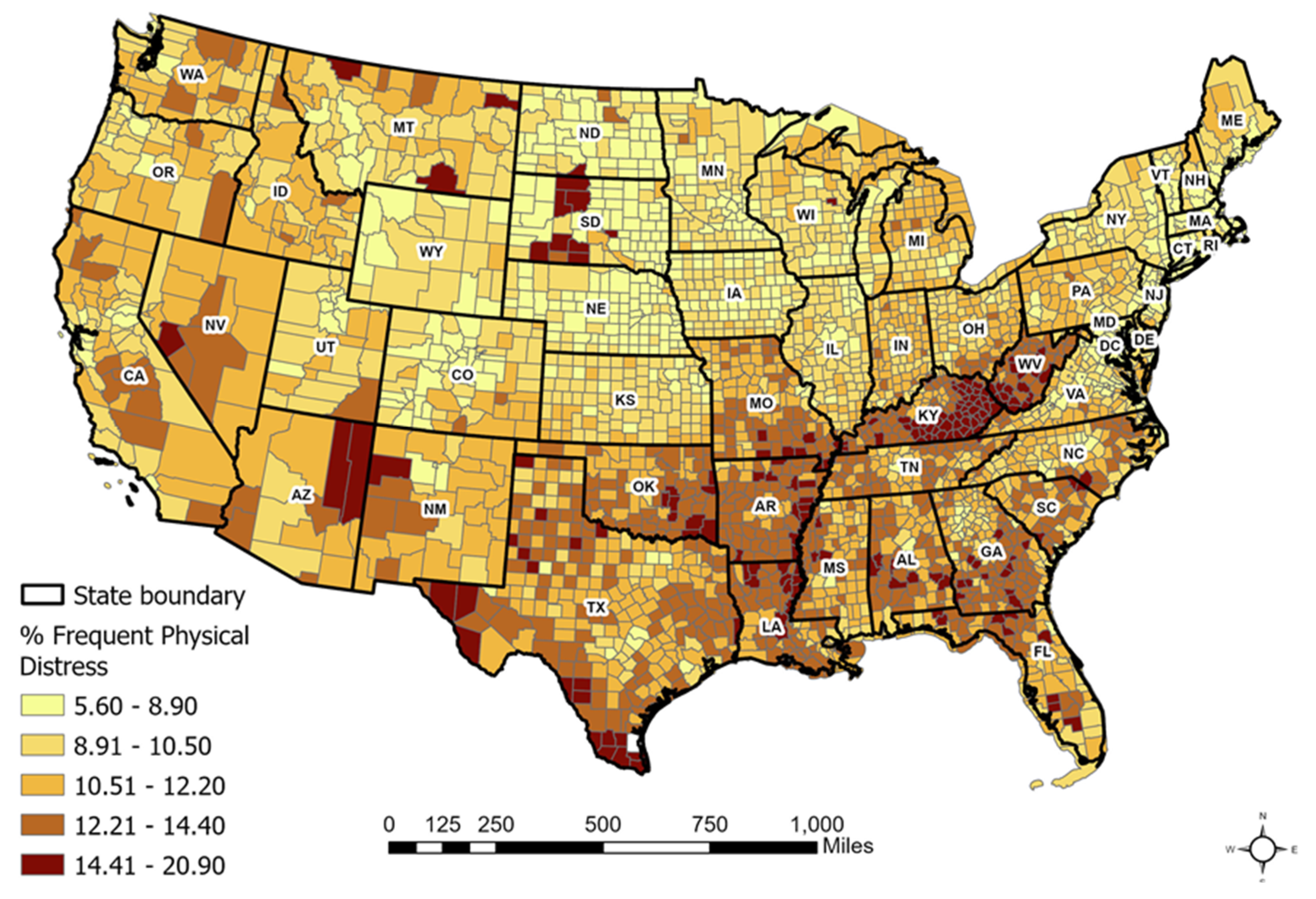
Figure 2.
Coefficient estimates of the MGWR model: (a) food environment index; (b) percentage of insufficient sleep; (c) percentage of college education; (d) association rate; (e) median household income; (f) percentage of African American.
Figure 2.
Coefficient estimates of the MGWR model: (a) food environment index; (b) percentage of insufficient sleep; (c) percentage of college education; (d) association rate; (e) median household income; (f) percentage of African American.
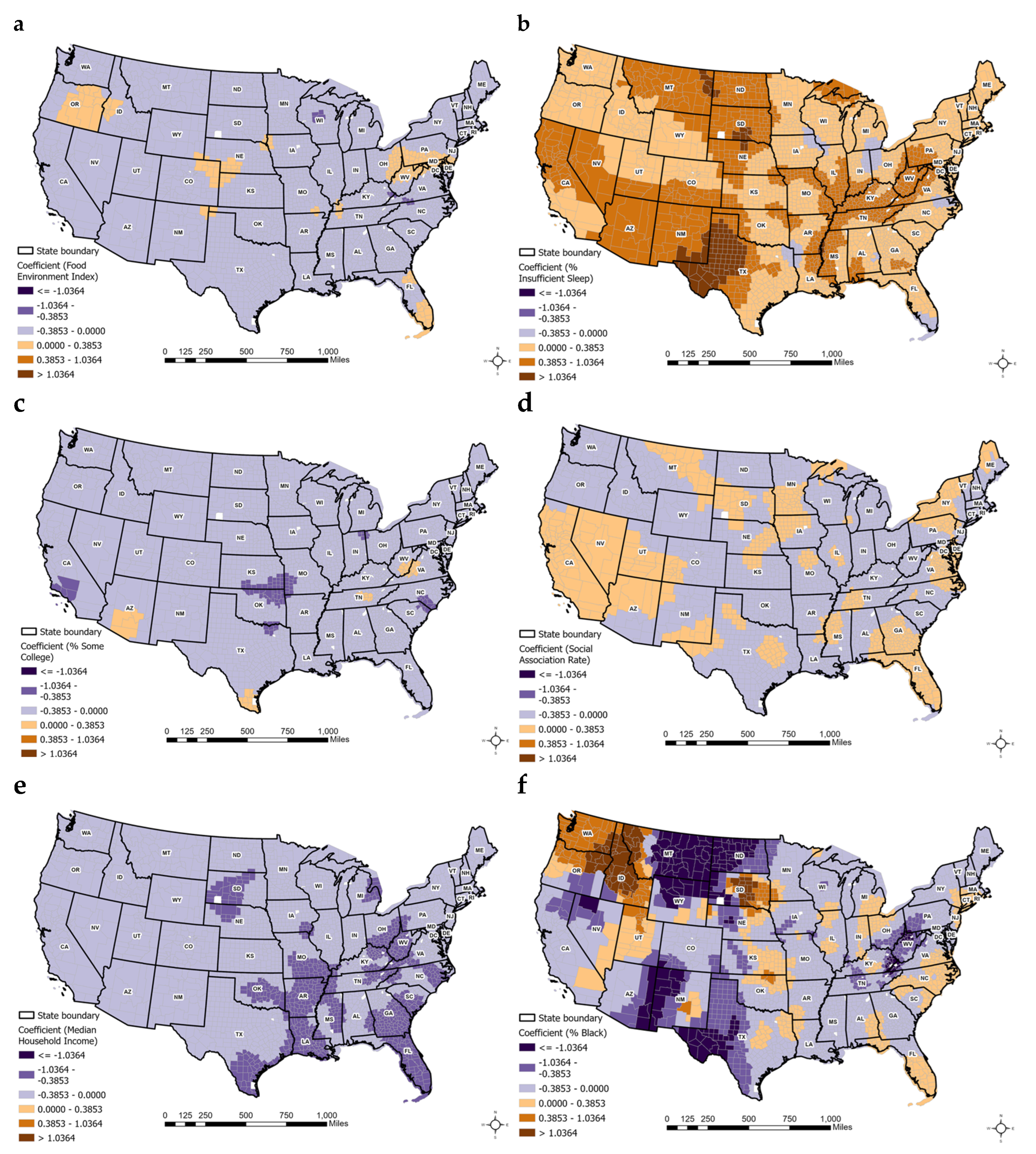
Figure 3.
Significance map of MGWR model: (a) food environment index; (b) percentage of insufficient sleep; (c) percentage of college education; (d) association rate; (e) median household income; (f) percentage of African American.
Figure 3.
Significance map of MGWR model: (a) food environment index; (b) percentage of insufficient sleep; (c) percentage of college education; (d) association rate; (e) median household income; (f) percentage of African American.
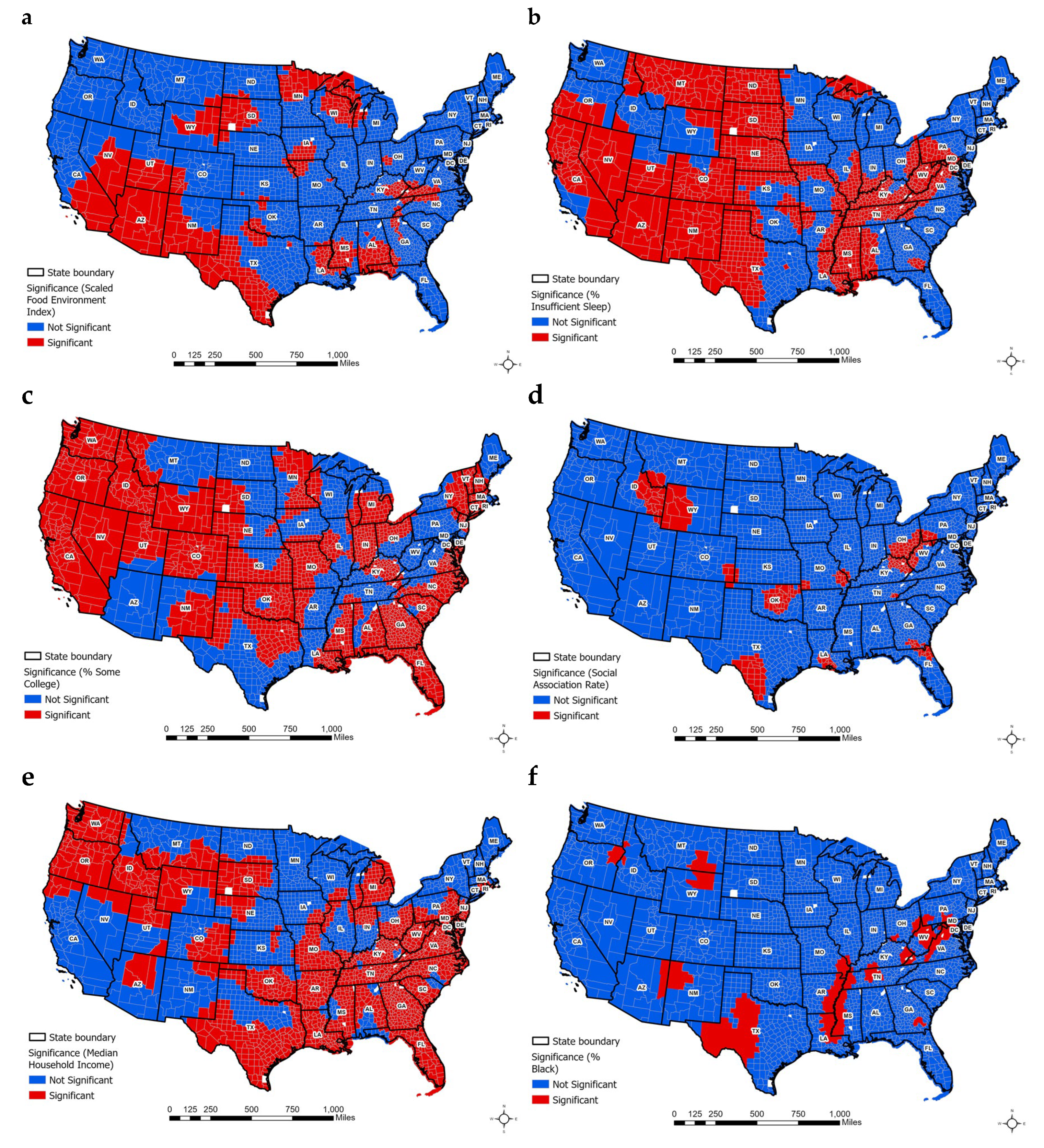

Table 1.
Descriptive and bivariate statistics for dependent and independent variables.
| N | Mean | SD | Bivariate | |
|
Dependent variable: Frequent Physical Distress (FPD) |
2673 |
10.942 |
2.083 |
1.000** |
| Independent variables: | ||||
| Health behaviors: | ||||
| % adult smoking | 2673 | 19.983 | 4.004 | 0.823** |
| % adult obesity | 2673 | 36.187 | 4.674 | 0.671** |
| Food environment index | 2673 | 7.502 | 1.058 | -0.675** |
| % physically inactive | 2673 | 25.627 | 5.088 | 0.877** |
| % with access to exercise | 2673 | 63.732 | 21.258 | -0.455** |
| % alcohol impaired | 2673 | 19.034 | 3.174 | -0.548** |
| % insufficient sleep | 2673 | 34.591 | 3.591 | 0.727** |
| Clinical care: | ||||
| % uninsured | 2673 | 11.511 | 5.029 | 0.449** |
| Primary care physician ratio | 2673 | 55.215 | 34.400 | -0.388** |
| Mental health provider rate | 2673 | 191.972 | 192.908 | -0.181** |
| Preventable hospitalization rate | 2673 | 3015.104 | 1112.770 | 0.489** |
| Social economic environment: | ||||
| % of college education | 2673 | 58.984 | 11.296 | -0.764** |
| % unemployment | 2673 | 4.710 | 1.655 | 0.352** |
| Association rate | 2673 | 11.453 | 4.684 | -0.195** |
| Median household income | 2673 | 59606.975 | 15553.751 | -0.762** |
| Demographics: | ||||
| % 65 and over | 2673 | 19.716 | 4.554 | 0.002 |
| % African American | 2673 | 9.574 | 14.282 | 0.269** |
| % Female | 2673 | 49.782 | 1.975 | -0.027 |
| % Rural | 2673 | 53.376 | 29.675 | 0.306** |
| Abbreviation: SD, Standard Deviation; **Significant at p>0.05 | ||||
Table 2.
OLS analyses of explanatory variables for FPD.
| Coefficient | S.E | t-value | p-value | 95% C.I | VIF | |||
| Model 1- Adjusted R2: 0.855 | Lower Bound | Upper Bound | ||||||
| Constant | 10.183 | 0.607 | 16.786 | 0.000 | 8.993 | 32.580 | ||
| Health behaviors: | ||||||||
| % adult obesity | 0.040 | 0.006 | 7.294 | 0.000** | 0.029 | 0.051 | 2.834 | |
| Food environment index | -0.305 | 0.022 | -14.116 | 0.000** | -0.348 | -0.263 | 2.229 | |
| % with access to exercise | -0.001 | 0.001 | -1.333 | 0.183 | -0.004 | 0.001 | 2.313 | |
| % alcohol impaired | -0.054 | 0.007 | -8.117 | 0.000** | -0.067 | -0.041 | 1.895 | |
| % insufficient sleep | 0.154 | 0.007 | 20.590 | 0.000** | 0.139 | 0.169 | 3.070 | |
| Clinical care: | ||||||||
| % uninsured | 0.033 | 0.004 | 8.733 | 0.000** | 0.025 | 0.040 | 1.521 | |
| Primary care physician ratio | 0.002 | 0.001 | 3.270 | 0.001** | 0.001 | 0.003 | 1.670 | |
| Mental health provider rate | 0.000 | 0.000 | 3.027 | 0.002** | 0.000 | 0.000 | 1.513 | |
| Preventable hospitalization rate | 9.523E-5 | 0.000 | 5.669 | 0.000** | 0.061 | 0.094 | 1.487 | |
| Social economic environment: | ||||||||
| % of college education | -0.042 | 0.002 | -17.278 | 0.000** | -0.047 | -0.037 | 3.218 | |
| % unemployment | 0.068 | 0.011 | 6.044 | 0.000** | 0.046 | 0.090 | 1.474 | |
| Association rate | -0.042 | 0.004 | -11.086 | 0.000** | -0.050 | -0.035 | 1.348 | |
| Median household income | -3.755E-5 | 0.000 | -21.451 | 0.000** | 0.000 | 0.000 | 3.155 | |
| Demographics: | ||||||||
| % 65 and over | -0.040 | 0.005 | -8.898 | 0.000** | -0.049 | -0.032 | 1.829 | |
| % African American | -0.025 | 0.001 | -17.924 | 0.000** | -0.028 | -0.022 | 1.664 | |
| % Female | -0.044 | 0.009 | 4.875 | 0.000** | 0.026 | 0.061 | 1.334 | |
| % Rural | 0.006 | 0.001 | 6.475 | 0.000** | 0.004 | 0.007 | 2.882 | |
| Abbreviation: SE, Standard Error; **Significant at p>0.05 | ||||||||
Table 3.
GWR and MGWR analyses of explanatory variables for FPD.
| Coefficient Range | |||||||||
| Model 2- Adjusted R2: 0.912 (GWR); AICc: 1,671.088 | |||||||||
| Model 3- Adjusted R2: 0.918 (MGWR); AICc: 1,633.507 | Mean | S.D | Minimum | Maximum | Optimal Neighbors (% of features) |
Significance (% of features) |
|||
| Intercept | -0.102 | 0.432 | -4.282 | 2.382 | 103 (3.35) | 798 (25.94) | |||
| Health behaviors: | |||||||||
| Food environment index | -0.134 | 0.094 | -0.441 | 0.177 | 120 (3.90) | 622 (20.22) | |||
| % insufficient sleep | 0.382 | 0.295 | -0.210 | 1.773 | 108 (3.85) | 1495 (48.60) | |||
| Social economic environment: | |||||||||
| % of college education | -0.211 | 0.088 | -0.547 | 0.059 | 132 (4.29) | 1858 (60.40) | |||
| Association rate | -0.039 | 0.087 | -0.367 | 0.206 | 135 (4.39) | 252 (8.19) | |||
| Median household income | -0.309 | 0.147 | -0.829 | -0.024 | 121 (3.93) | 1902 (61.83) | |||
| Demographics: | |||||||||
| % African American | -0.186 | 0.635 | -7.324 | 3.874 | 101 (3.28) | 330 (10.73) | |||
| Abbreviation: SD, Standard Deviation; **Significant at p>0.05 | |||||||||
Disclaimer/Publisher’s Note: The statements, opinions and data contained in all publications are solely those of the individual author(s) and contributor(s) and not of MDPI and/or the editor(s). MDPI and/or the editor(s) disclaim responsibility for any injury to people or property resulting from any ideas, methods, instructions or products referred to in the content. |
© 2025 by the author. Licensee MDPI, Basel, Switzerland. This article is an open access article distributed under the terms and conditions of the Creative Commons Attribution (CC BY) license (https://creativecommons.org/licenses/by/4.0/).
Copyright: This open access article is published under a Creative Commons CC BY 4.0 license, which permit the free download, distribution, and reuse, provided that the author and preprint are cited in any reuse.


