
Submitted:
10 December 2025
Posted:
12 December 2025
You are already at the latest version
Abstract
The increasing adoption of highly variable renewable energy has introduced unprecedented volatility into the National Electricity Market (NEM), rendering traditional linear price forecasting models insufficient. The Australian Energy Market Operator (AEMO) spot price forecasts often struggle during periods of volatile demand, renewable variability, and strategic rebidding. This study evaluates whether transformer architectures can improve intraday NEM price forecasting. Using 34 months of market data and weather conditions, several transformer variants, including encoder–decoder, decoder-only, and encoder-only, were compared against the AEMO’s operational forecast, a two-layer LSTM baseline, the Temporal Fusion Transformer, PatchTST, and TimesFM. The decoder-only transformer achieved the best accuracy across the 2–16 hour horizons in NSW, with nMAPE values of 33.6–39.2%, outperforming both AEMO and all baseline models. Retraining in Victoria and Queensland produced similarly strong results, demonstrating robust regional generalisation. A feature importance analysis showed that future-facing predispatch and forecast covariates dominate model importance, explaining why a decoder-only transformer variant performed so competitively. While magnitude estimation for extreme price spikes remains challenging, the transformer models demonstrated superior capability in delivering statistically significant improvements in forecast accuracy. An API providing real-time forecasts using the small encoder-decoder transformer model is available at https://nem.redaxe.com
Keywords:
electricity price forecasting
; national electricity market (NEM)
; transformer models
; deep learning
; intraday forecasting
; energy market modelling
; market volatility
; temporal feature engineering
; machine learning applications in energy
; Australian energy markets
1. Introduction
As the world embraces renewable energy and associated energy storage systems, the ability to accurately forecast electricity prices is becoming increasingly important. Investment in renewable energy projects relies on financial returns, which are enhanced by predictable energy prices.
In the case of electricity in Australia, spot prices are determined by two energy markets - the National Electricity Market (NEM) and the Wholesale Electricity Market (WEM). The NEM serves the eastern states, and the majority of the Australian population, while the WEM exclusively serves the state of Western Australia (WA). The NEM is managed by the Australian Energy Market Operator (AEMO).
The NEM Regional Reference Price (RRP) forecasts are currently created using a linear programming solver that takes electricity generator price bids and forecast demand and solves for the minimum cost solution per five minute period [1]. A linear programming solver aims to solve a set of linear equations in the following mathematical form:
In this case, Z represents the total costs, c represents the generator bids and x is the power dispatched to the generator at their bid price. The constraints such as forecast demand, generator ramp time and interconnector constraints would be represented by a, xj and b.
Typically, generators will initially bid high and then lower their bids as they approach the five minute execution period in order to secure the right to deliver their energy for the period [2]. Consequently, NEM price forecasts often start high and usually decrease as the delivery time approaches.
Forecasts of NEM spot prices are widely utilised by a diverse range of stakeholders. Generation companies, including coal, gas, hydro, solar, and wind operators, draw upon such forecasts to determine optimal dispatch, storage, and curtailment strategies. Battery storage operators employ forecast information to inform charging, discharging, and energy-holding decisions, thereby maximising revenue while maintaining system reliability. Retail electricity providers use price forecasts to develop hedging strategies aimed at mitigating exposure to wholesale price volatility. Similarly, Virtual Power Plant (VPP) operators incorporate forecasts into scheduling algorithms that determine when distributed resources should buy from or sell to the grid [3]. Large commercial and industrial consumers may rely on forecasts to schedule flexible demand or to manage financial risk through hedging instruments. In parallel, speculative traders in the Australian Securities Exchange (ASX) energy futures market employ forecast data to identify opportunities for arbitrage and portfolio optimisation [4].
The consequences of forecast inaccuracy are therefore far-reaching. Poorly calibrated or unreliable spot price forecasts can negatively impact generation scheduling, storage dispatch, retail risk management, and demand-side planning. These inefficiencies ultimately propagate across the market, raising transaction costs, reducing allocative efficiency, and contributing to higher electricity prices for all consumers. Consequently, improving forecast accuracy remains a critical research and policy priority for electricity markets undergoing rapid transitions in generation mix, demand flexibility, and storage integration.
More broadly, improved price forecasts will lead to more efficient use of electricity. This, in turn, will put downward pressure on electricity prices and benefit the entire economy. Lower electricity prices will provide social benefits to low income families that may be struggling with cost of living pressures. Energy efficiency is critical for the environment because energy production has a negative environmental impact, regardless of whether or not it is renewable [5].
1.1. Related Works
Approaches to price forecasting include both traditional statistical methods, such as Auto-Regressive Integrated Moving Average (ARIMA) [6] or multiple linear regression [7] and conventional modern machine learning techniques. The latter include gradient boosting machines [8] or deep learning techniques such as Long-Short Term Memory (LSTM) Recurrent Neural Networks (RNNs) [9,10,11]. Recent work has begun to explore transformer-based approaches for financial and energy-related forecasting, although these studies remain limited in scope. For example, Hartanto and Gunawan [12] applied the Temporal Fusion Transformer to multivariate stock price prediction and demonstrated that the model could capture complex temporal patterns more effectively than recurrent neural network baselines. Their study emphasised the benefits of combining transformer attention mechanisms with LSTM-style sequence modelling, aligning with much of the broader literature in which hybrid Convolution Neural Network (CNN)–LSTM or CNN–BiLSTM architectures continue to dominate forecasting research.
Many recent approaches to electricity prediction rely on LSTMs or use hybrid rather than pure transformer methods, which makes it difficult to gain insight into the potential effectiveness of end to end transformers applications. For example, Lago et al. performed a review of state-of-the-art algorithms used to predict day-ahead electricity prices for markets where generator bids are submitted for a full day of delivery [13]. They found the Deep Neural Network, a multilayer perceptron with 2 hidden layers, to slightly outperform LSTMs and Gated Recurrent Units (GRU) in terms of price predictions by deep learning models. However, it did not consider transformer-based deep learning models. Similarly, in 2022, Bottieau et al. studied a novel LSTM/transformer hybrid approach for predicting real-time pricing of the Belgian electricity market [14]. Their model featured a set of bidirectional LSTMs and was combined with a single self-attention mechanism. Bidirectional LSTMs were utilised to provide the temporal processing layer, and the self-attention mechanism then provided the attention focus. Their approach, which compared their hybrid model to traditional LSTMs, ARMAX, and gradient boosted trees, was effective in that their model outperformed the selected “state-of-the-art forecasting” methods. However, it did not research how a traditional, full encoder-decoder transformer performed. Abdellatif et al. investigated hybrid deep learning architectures for day-ahead forecasting in the Nord Pool electricity market, combining a Bidirectional LSTM (BiLSTM) with Convolutional Neural Network (CNN) layers to leverage both local pattern extraction and long-range temporal dependencies [15]. To address scale sensitivity in neural network forecasting models, particularly the difficulty neural components have when predictor variables operate on very different numerical ranges, they incorporated a linear autoregressive bypass that learns a direct mapping from recent prices to future values. This hybrid architecture, termed CNN-BiLSTM-AR, was evaluated against several alternatives including CNN-LSTM, CNN-BiLSTM, and CNN-LSTM-AR. Across multiple error metrics, their results showed that the CNN-BiLSTM-AR model consistently achieved the lowest forecasting errors, demonstrating the benefit of combining convolutional feature extraction, bidirectional sequence modelling, and an autoregressive linear path within a single framework.
Some studies used either a transformer-based encoder, but neglected to use the decoder with future covariates. For example, Cantillo-Luna et al. researched a probabilistic model based on transformer encoder blocks with Time2Vec [16] layers to predict electricity prices eight hours ahead in the Colombian market [9]. They compared their model to models such as Holt–Winters, XGBoost, Stacked LSTM, and an Attention-LSTM hybrid, and successfully demonstrated that their model outperforms these traditional approaches. However, they did not study the performance of a full encoder-decoder model, and they only assessed 8-hour-ahead predictions.
Of particular relevance to this study is Tan et al and Ghimire et al. which both addressed the Australian NEM. Tan, et al. performed a study by applying a CNN and a sparse encoder to the NSW1 NEM region [17]. They employed an ensemble approach by incorporating a decomposition function into the complex time series to mitigate noise and volatility. They successfully showed that such an ensemble was an effective approach to NEM spot price predictions. Ghimire et al. published a study in 2024 that aimed to predict 30-minute electricity prices in the NSW1 NEM region, utilising a hybrid MoDWT (Maximum Overlap Discrete Wavelet Transform) decomposition technique with a Bayesian-optimised CNN [18]. They found that, when compared to traditional models such as Bi-LSTM, LSTM, random forest, extreme gradient boosting, and multi-layer perceptron, the hybrid CNN model produced superior results. While both of these studies examined the application of deep learning techniques to NEM spot prices, they did not explore transformer-based models nor did they benchmark against the NEM operational forecast or show generalisation to other NEM regions.
Several recent papers have examined related problems that further highlight the emerging role of transformer architectures in electricity markets. One study developed a transformer-based price forecasting system with SHAP interpretability, showing that attention mechanisms combined with feature attribution can reveal the dominant drivers of electricity price variation while achieving strong predictive accuracy [19]. Another study focused on predicting extreme price events by integrating fine tuned large language models with wavelet enhanced CNN LSTM architectures, demonstrating that structured information extracted from AEMO market notices can meaningfully improve forecasts during volatile periods in the NEM [20]. Work by Malyala et al. introduced a hybrid Graph Patch Informer and Deep State Sequential Memory approach for state wide energy markets, showing that reliable forecasts can be achieved using only price and demand without weather inputs, which often add noise at broader geographic scales [21].
Beyond forecasting, transformer based temporal feature extraction has also been applied to operational decision making, such as a temporal aware reinforcement learning framework that enables battery energy storage systems to optimise joint participation in the spot and contingency Frequency Control Ancillary Services (FCAS) markets, demonstrating substantial revenue gains through improved modelling of temporal price patterns [22].
While recent studies have begun exploring transformer architectures for related forecasting tasks, such as Ghimire et al. who applied a transformer to load forecasting in Queensland in 2023 [23], and hybrid convolutional network approaches used for 30-minute price prediction in New South Wales in 2024, the broader literature on electricity price forecasting remains dominated by convolutional networks, recurrent networks, and ensemble methods. No existing studies evaluate the performance of pure transformer models, in particular the traditional encoder–decoder architecture, for electricity price forecasting in Australia or internationally. This represents an important methodological gap because wholesale electricity prices arise from the interaction of both demand and supply side bidding under rapidly changing market conditions, an environment that aligns naturally with the attention mechanisms and sequence modelling capabilities of transformers. The present study addresses this gap by evaluating state-of-the-art transformer architectures for the task of predicting volatile NEM spot prices, providing the first systematic assessment of transformer-only models for this forecasting domain.
2. Materials and Methods
2.1. Data
All data used in this study was obtained from publicly available sources, ensuring full reproducibility. Electricity market observations and forecast data were sourced from the Australian Energy Market Operator (AEMO) [24,25], while meteorological observations and forecasts were obtained from Open-Meteo [26]. Features were created for each NEM region, as shown in Figure 1, since they all form part of an interconnected energy market.
The data collected covered 30 minute periods from November 2022 through to August 2025 and featured 49,447 observations in total. The consolidated multivariate dataset created for this research has been deposited as an open-access resource1. All preprocessing scripts, model configurations, and training code are also publicly available.2 A schematic overview of the data pipeline is provided in Figure 2.
2.2. Preprocessing
Thirty-four months of data was collected, covering NEM operational information, including actual spot prices, operational demand and net interchange, as well as the full suite of NEM thirty-minute ahead pre-dispatch forecasts for price, demand, and net interchange. Weather variables, including temperature, humidity, wind speed, and cloud cover, were compiled for the capital city associated with each NEM region examined in this study. As no official benchmark dataset exists for NEM forecasting research, all data streams were manually merged into a consistent temporal frame.
All data was resampled or aggregated to a uniform thirty-minute resolution, ensuring strict timestamp alignment across the actual and forecast domains. Preprocessing involved parsing and flattening nested AEMO files, resolving daylight savings irregularities, removing anomalies, interpolating missing meteorological measurements as necessary, and producing a final, chronologically ordered dataset. No temporal shuffling occurred prior to dataset splitting.
Feature engineering aimed to provide the models with variables known or hypothesised to influence NEM price formation [17,28]. These included time-based encodings capturing diurnal, weekly, and seasonal cycles. Weather features that were expected to have the greatest impact on regional electricity generation and consumption were chosen. RRP, demand and net interchange features were included for all NEM regions since they are all interconnected and influence prices in each. The complete list of features used is shown in Table 1.
2.3. Model Architectures
The primary forecasting model used in this study was a transformer architecture based on the seminal work of Vaswani et al. [29], as illustrated in Figure 3. Transformers make use of a multi-head self-attention mechanism in which attention heads learn to emphasise the most relevant parts of the input sequence at each timestep. This mechanism enables efficient modelling of long-range temporal dependencies, making transformers particularly effective for electricity price forecasting where patterns can span multiple hours or even days.
Transformers typically consist of an encoder and a decoder linked by a cross-attention mechanism. The encoder processes the historical sequences, such as RRP, demand, and weather actuals, while the decoder consumes the known future inputs, including AEMO pre-dispatch forecasts and weather forecasts. Both components may be stacked in multiple layers to provide increased representational capacity and enable the model to capture hierarchical temporal patterns across different forecast horizons.
In this study, the encoder was responsible for learning latent representations of past market behaviour, whereas the decoder integrated these representations with exogenous forward-looking signals to generate a full 16-hour ahead forecast. Positional encodings were applied to both streams to ensure that the model retained awareness of the temporal order of the inputs, a crucial requirement given the irregular and highly dynamic nature of NEM spot prices. The combination of multi-head self-attention, cross-attention, and deeply stacked layers allowed the model to capture nonlinear interactions between historical drivers, forecast inputs, and evolving system conditions more effectively than recurrent or convolutional baselines.
Since the original transformer was developed for sequence-to-sequence text translation, several modifications were made to adapt the architecture for numerical time-series forecasting and to improve training stability on NEM datasets. First, a pre-layer normalisation (pre-LN) formulation was adopted, following the stabilised architecture proposed by Wang et al. [30]. Pre-LN significantly improves gradient stability during training and removes the need for the large learning-rate warm-up schedule used in the original transformer. Consequently, the warm-up phase was omitted entirely, and the model was successfully trained using the standard Adam optimiser [31] with a fixed learning rate.
Second, the decoder was configured to use parallel decoding, enabling the model to generate the entire 32-step forecast horizon in a single forward pass. This approach avoids the accumulation of error inherent in autoregressive decoding and aligns with operational forecasting needs in the NEM, where full multi-horizon price trajectories must be generated simultaneously. To assess the impact of decoding strategy, an additional autoregressive (AR) decoder variant was implemented and evaluated. The AR configuration predicted each future timestep sequentially, feeding earlier predictions back into the model, enabling direct comparison between parallel and AR decoding methods.
The default “small” encoder–decoder model consisted of three layers with four attention heads per layer, a hidden dimension of 128, a feed-forward dimension of 512, and a dropout rate of 0.05. It accepted an input sequence of ninety-six 30-minute time steps and produced a forecast horizon of thirty-two 30-minute time steps.
To evaluate robustness and generalisation, a variety of architectural variants were tested, including tiny, small, medium, and large transformer models, as well as encoder-only and decoder-only configurations. A summary of these variants and their hyperparameters is provided in Table 2 and shown in Figure 4.
A generic two-layer Long Short-Term Memory (LSTM), a Patch Time Series Transformer (PatchTST) [32], a TimesFM [33], and a Temporal Fusion Transformer (TFT) [34], were included for comparison. These models were chosen since they were modern state-of-the-art hybrids of each kind of transformer. TimesFM is a decoder-only model, PatchTST is encoder-only, and TFT contains both encoders and decoders. The architectures of each of these are shown in Figure 5.
A simple two-layer LSTM provides a strong baseline for short-term RRP forecasting because it captures sequential dependencies in load, price, and weather while remaining computationally lightweight. The first LSTM layer learns short term patterns, such as daily patterns, while the second layer captures longer term patterns including weekly and seasonal changes. LSTMs are the currently established way of solving these types of time-series problems [10,11].
The TFT architecture combines LSTM encoders with multi-head attention and explicit variable-selection layers, making it well-suited to RRP forecasting, where both past conditions and future covariates, such as predispatch forecasts, weather projections, and outages, influence price formation. Its LSTM layers learn local patterns, and its attention mechanisms help identify which drivers matter at longer horizons, giving good interpretability and often strong performance when diverse feature sets are available. The traditional quantile output head has been replaced with a single dense output head since we are doing point-price predictions.
TimesFM applies a pretrained large-scale foundation model with self-attention encoders and a dedicated forecast head, allowing it to extract generalisable temporal patterns from NEM data. Its ability to transfer patterns learned from massive global time-series corpora makes it effective for medium-horizon RRP prediction, where structural noise, demand cycles, and renewable variability dominate. It is used in zero-shot mode, without any fine-tuning, where it can generate accurate multi-step forecasts by conditioning only on the input sequence and forecast horizon, making it highly adaptable to unseen time series with minimal task-specific configuration. However, it has the potential for improvement with fine-tuning.
PatchTST excels in RRP forecasting by processing inputs as overlapping temporal patches, allowing the model to focus on localised variations, such as ramp events, solar troughs, wind lulls, and rebidding episodes, while efficiently capturing long-range structure through attention. Its channel-independent design, in which each feature is viewed in its own channel, cleanly handles multivariate NEM inputs and often improves robustness, particularly when the target series exhibits nonlinear seasonality or regime changes.
2.4. Training Procedure and Hyperparameter Tuning
The 2-layer LSTM and TFT models were implemented using Keras 3.12 and Tensorflow 2.16. PatchTST was implemented with Pytorch 2.9 and TimesFM inference was performed with the pre-trained Pytorch model [35]. All models were trained using an 80:20 train:test split, ensuring that the hold-out test set comprised exclusively unseen future data. The training dataset consisted of 37,085 observations with a validation set of 2,440 observations. The hold-out test dataset was 9,858 observations. Temporal integrity was strictly preserved by avoiding any form of shuffling before the split and a padded zone was added between sets to ensure no data leakage between any of the sets. After partitioning, the training set was shuffled at the sequence level to reduce the risk of memorisation. Experiments were executed using Nvidia A100 GPU-accelerated compute resources. Random seeds were fixed for all runs to guarantee deterministic behaviour. Prior to training, inputs were scaled using a quantile transformer (normal output distribution, 2000 quantiles) to handle the heavy-tailed and non-Gaussian characteristics of NEM price data. PatchTST was the only exception and utilised a robust scaler for input scaling since it produced better results during tuning.
Hyperparameters, including model depth, attention heads, dropout, feed-forward dimensionality, input sequence length, and optimiser configuration, were tuned using a five-fold walk-forward validation procedure. This method allowed the models to be trained and validated on sequentially advancing windows that mimicked real operational forecasting constraints. The final hyperparameter selections for each model are summarised in Table 3.
2.5. Evaluation Framework
Model performance was evaluated at discrete forecast horizons ranging from 2 to 16 hours ahead. The primary metrics were Normalised Mean Absolute Percentage Error (nMAPE) and Mean Absolute Error (MAE):
In addition, forecasts were benchmarked directly against AEMO’s published pre-dispatch values to assess operational improvement potential. Initial experiments focused on the NSW1 region, after which the models were retrained and applied to the VIC1 and QLD1 regions using identical feature sets except for region-specific weather inputs.
3. Results
In this section, we provide performance results for all transformer architectures for the NSW1, VIC1, and QLD1 datasets. In Table 4, we compare the performance of each transformer architecture against the NEM operational forecast and the comparison models across 2-16 hour horizons on the NSW1 dataset. We present SHAP analysis results for the transformer models to understand which features contribute to performance. We then provide results for two other NEM regions, QLD1 and VIC1, to show the generalisability of the transformer models.
For the NSW1 NEM region, the decoder-only transformer architecture consistently outperformed all other models, demonstrating significant improvements in forecast accuracy. As shown in Table 4 and Figure 6, the decoder-only transformer achieved the strongest short-range performance, with nMAPE values of 33.6% to 39.2% across all horizons. Compared to the official NEM predispatch forecast, which reported nMAPE values between 65.6% and 116.0%, this represents a 46–67% reduction in forecast error, a magnitude of improvement that is both substantial and statistically significant in the context of electricity price forecasting as confirmed by a Diebold-Mariano test (Table 8).
The Temporal Fusion Transformer (TFT) was the next-best-performing model overall, achieving nMAPE values of 36.3% to 40.8% across the forecast horizons. The LSTM baseline displayed competitive short-term performance (e.g., 38.2% at 2 hours), but degradation accelerated with the forecast horizon, ending at 44.4% at 16 hours. While the LSTM achieved 30–60% lower error than the NEM baseline, it remained 5–15% worse than the leading transformer models across most horizons. Such differences are large enough to be considered practically meaningful in operational settings where small improvements translate directly into improved dispatch and arbitrage outcomes. From a consistency across forecast horizons perspective, Figure 7 shows that the encoder–decoder and the autoregressive transformer variants achieved consistently low MAE values, while TimesFM in a zero-shot mode exhibited the highest higher error dispersion of the non-NEM forecasts. The NEM forecasts had the greatest range of MAE values showing very inconsistent accuracy.
3.2. SHAP Results
The SHAP-based feature importance analysis [36], performed for the small enc-dec transformer model on the NSW region and shown in Figure 8, shows a clear and consistent pattern: future-facing decoder inputs dominate predictive power, while historical encoder features contribute relatively little to the model’s accuracy. In the NSW1 analysis, the most influential features were overwhelmingly the AEMO predispatch forecasts, led by the NSW1 NEM RRP forecast, which contributed more than 60% of the total importance. Forecasted regional demand, interconnector flows, and multi-region forecast RRPs also ranked highly, confirming that the transformer relies primarily on market expectations and system outlooks rather than long-range historical patterns.
In contrast, the encoder-side historical features all exhibited very small contributions, each accounting for only a few percent of total importance. These included past RRPs, historical regional demands, weather observations, and cyclical time encodings. Their uniformly low impact is consistent with the model architecture and the structure of the NEM. Once future-facing covariates such as AEMO predispatch forecasts are available, historical inputs add little incremental value for multi-hour-ahead price prediction.
3.3. Region Generalisation Results
Across all three NEM regions, the transformer-based models exhibited highly consistent forecasting behaviour, with error profiles that closely mirrored those obtained in the NSW1 experiments as shown in Table 5, Figure 9, Table 6 and Figure 10. In both QLD1, the decoder-only and encoder–decoder transformers again produced the strongest overall results, maintaining nMAPE values in the low 30 percent range across the 2–16 hour horizons. This stability across markets with markedly different generation mixes, levels of renewable variability, and interconnector dynamics indicates that the learned representations generalise effectively beyond the original NSW1 training environment. The only notable exception occurred in VIC1 at the two-hour horizon, where the official NEM forecast marginally outperformed all machine learning models. At all other horizons in VIC1, and at every horizon in NSW1 and QLD1, the transformer variants remained superior to the NEM benchmark. Models such as the TFT performed well, especially in VIC1, but was less consistent in QLD1, while historical-only approaches, including PatchTST and TimesFM, performed substantially worse. Overall, the cross-regional consistency of the transformer models suggests a strong capacity to capture structural patterns in NEM price formation and indicates clear potential for generalisable, real-time forecasting applications.
3.4. Transformer Size Variant Results
Across the model-size comparison, the small encoder–decoder transformer achieved the lowest nMAPE values for NSW1 for the 2-hour and 4-hour horizons, outperforming both smaller and larger variants across all horizons as shown in Table 7. It was second to the large model for the other horizons but the difference was less than 1%. These results indicate that the small configuration provides the best balance between model capacity and dataset size. The medium model offered no increase in accuracy despite having higher internal dimensions, whereas the large model, with an extra layer and twice as many attention heads, provided the better performance at longer forecast horizons.
4. Discussion
4.1. NSW1 Region Performance
The encoder-decoder and decoder-only transformers performed particularly well on this dataset because their architecture naturally accommodates multi-source, heterogeneous inputs, allowing the model to integrate AEMO predispatch forecasts, weather outlooks, and other forward-looking signals in a structured way. Unlike other deep learning models designed to take historical data only such as TimesFM and PatchTST, the encoder-decoder and decoder-only transformers handle future covariates and multi-step decoder inputs natively, enabling them to form richer representations of expected system conditions that extend well beyond the observed past. This aligns with the SHAP analysis, which indicates that the decoder-side features and forecast covariates dominate predictive importance, meaning the model gains most of its explanatory power from understanding future market expectations, not from long-range attention over historical sequences. The encoder-decoder transformers are particularly effective in this setting because they can represent these multi-horizon forecasts jointly while maintaining flexibility across different input types and time scales.
TFT’s strong performance largely reflects its ability to dynamically select and weight exogenous covariates, which suits the NEM where prices depend heavily on volatile inputs such as predispatch forecasts, weather features, and rooftop PV expectations. Its hybrid design, combining LSTMs for short-term structure with attention for longer-range dependencies, also helps it capture the mix of intraday and multi-hour patterns characteristic of electricity markets. Although it does not quite match the top-performing transformer variants, the difference is small (typically 1–3 percentage points), indicating that TFT remains a highly competitive model for operational price forecasting in the NEM.
Models relying solely on historical data, such as PatchTST and TimesFM, performed substantially worse. PatchTST achieved nMAPE values between 57.2% and 64.3%, while TimesFM exceeded 100% error at several horizons. These models performed 20–50% worse than the models using exogenous known forecast information, confirming that covariates such as AEMO predispatch forecasts, engineered temporal features, and weather forecasts are statistically essential for accurate electricity price prediction in the NEM. Their poor performance highlights the limitations of historical-only models in markets dominated by structural regime shifts, intervention events, and variable renewable output. This was confirmed by the SHAP study results which support the finding that models that are capable of using multivariate known forecasts are inherently better suited to NEM forecasting, as they directly ingest the information sources that contain the bulk of the explanatory power.
Across all models evaluated, including the transformer variants, the LSTM, the Temporal Fusion Transformer, PatchTST, and TimesFM, a consistent pattern emerged in the handling of extreme price events. The models generally identified the timing of price spikes but tended to under estimate their magnitude. This behaviour is expected in the National Electricity Market, where extreme price events are rare, heavy tailed, and contribute very little to the overall optimisation objective during training. As a result, models that minimise mean absolute error learn to prioritise accuracy on the far more frequent low and moderate price levels, and consequently regress toward central values when encountering rare extremes as shown in Figure 11. In contrast, the AEMO predispatch forecast, which is driven by operational risk considerations, often over predicts the height of price spikes. The transformer models therefore reflect the empirical structure of the training data rather than the cautious posture of an operational planning tool. This behaviour is characteristic of deep learning models trained on highly imbalanced and volatility dominated time series. Accurate price spike prediction remains an outstanding challenge, and there is often a trade-off between accurately forecasting regular daily price levels and anomalies.
The statistical significance of these results is demonstrated by the Diebold-Mariano tests presented in Table 8, where the improvement relative to the NEM forecast was evaluated for each model. These enhancements represent not only statistically significant improvements over the NEM benchmark at the 95 percent confidence level (p-value < 0.05) for all models but are also operationally relevant, considering the direct financial implications of forecast accuracy for battery dispatch, risk management, and market bidding strategies.
The improvement from an 82.7% nMAPE (as represented by the AEMO NEM price forecasts in NSW1 at the 4-hour horizon) to approximately 37% using the transformer-based model has significant implications for commercial battery operators. Profitability in battery arbitrage relies on accurately anticipating price differentials many hours in advance, since charge–discharge commitments, optimisation schedules, and market bids must be prepared well before real-time dispatch. An 82.7% forecast error forces operators to adopt highly conservative bidding strategies, often leading to missed revenue opportunities, suboptimal cycling, and increased exposure to unexpected price spikes. Reducing this error to around 37% fundamentally changes the operating landscape: the battery can commit to higher-confidence discharge events, avoid unnecessary charging during mispredicted low-price periods, and better position state-of-charge for periods of volatility. This improvement translates directly into increased arbitrage margins, more reliable charge and discharge decisions, and lower wear-related costs, because the battery can operate with far greater foresight rather than reacting to conditions as they occur. In practice, such a gain in predictive accuracy can yield materially higher annual returns, particularly in regions characterised by renewable-driven ramps and frequent intraday volatility, and positions the operator to compete more effectively against generators and traders who rely on less accurate public forecasts.
4.2. Generalisation to Other NEM Regions
Across all three NEM regions examined, the decoder-only transformer-based architecture displayed a striking level of consistency, suggesting a high degree of model generalisability despite the markedly different supply–demand profiles that characterise NSW1, QLD1 and VIC1. The strong results achieved in NSW1 were essentially replicated when the models were retrained on QLD1 and VIC1 targets. In QLD1, where price formation is heavily influenced by rooftop solar variability [23,37], rapid afternoon ramps and frequent strategic bidding, both the decoder-only and encoder–decoder transformers achieved error levels that closely matched those observed in NSW1. Similarly robust performance was obtained in VIC1, a region shaped by brown-coal baseload, interconnector congestion and different renewable generation patterns [37]. In each of these regions, the small decoder-only transformer consistently achieved normalised MAPE values in the upper thirties to very low forties across the 2–16 hour forecast horizons.
The fact that these models produced nearly identical accuracy distributions across three regions with such distinct load shapes, dispatch dynamics and renewable penetrations provides compelling evidence that the transformers did not simply overfit the NSW1 environment but instead learned structural relationships that transfer effectively across the broader NEM. This is further reinforced by the stability of model rankings across regions: the transformer variants remained the most accurate overall models in NSW1 and QLD1, and were either competitive with or superior to all other machine learning baselines in VIC1, with the main exception being the NEM’s own operational forecast at the 2-hour horizon, where it achieved the lowest error for that specific case.
The comparative models exhibited similar patterns across the three regions. The TFT and LSTM architectures maintained very good accuracy, though typically with slightly higher error ranges than the transformers except where the TFT dominated in VIC1. By contrast, historical-only models that lacked access to forward-looking covariates, including the encoder-only variant, PatchTST and TimesFM, consistently underperformed with greater errors in every region. It must be noted that TimesFM was used in a zero-shot capacity and may have performed better if it had been fine-tuned on the training dataset. AEMO’s official NEM forecasts also displayed considerably higher error levels at most horizons, particularly beyond short lead times, confirming that the market’s linear-programming-based forecasting engine struggles to match the representational capacity of the transformer architectures for intraday price prediction.
Taken together, the results across NSW1, QLD1 and VIC1 demonstrate that transformer-based models offer a reliable and transferable forecasting framework for the NEM. Their ability to reproduce strong performance across diverse regional conditions indicates that the learned temporal and cross-feature dependencies capture fundamental aspects of price formation that are stable across the eastern Australian grid. This suggests a high degree of practical generalisability and supports their potential for real-time deployment in operational forecasting, battery optimisation and market-facing analytics.
4.3. Transformer Variants
The size variant results in Table 7 show that the small encoder–decoder transformer provides the best overall performance for the NSW1 region, achieving nMAPE values of 34%–40% across the five evaluated forecast horizons. Although the tiny and medium variants produced competitive results, their accuracy was consistently inferior to the Small model by a margin of 1–2 percentage points at the shorter horizons where precision is most critical. The large model, with extra attention heads and layers, demonstrated superior performance at longer horizons but the small model stayed within 1% of it.
The relative stability of the small model across horizons indicates that it achieves the best balance between capacity and data availability for the NSW1 training set. NEM price data, although rich in covariates, remains highly volatile and structurally complex, with only limited signal available to support very deep or wide architectures. Larger models may be prone to learning noise or over-representing rare price regimes, while smaller models may lack sufficient representational power to encode multi-hour interactions between demand, renewables, and market expectations. The small model appears to sit at the optimal point on this trade-off curve, offering enough depth and width to model nonlinear interactions and multi-horizon dependencies without exceeding the dataset’s effective information content. Consequently, it represents the most suitable architecture for operational use in short- and medium-term price forecasting for the NSW1 region.
5. Conclusions
This study investigated the effectiveness of various transformer-based models for forecasting spot electricity prices in the Australian National Electricity Market. Using 34 months of AEMO market data, weather observations, weather forecasts, and engineered features, a set of transformer architectures was trained and evaluated under a walk-forward validation framework to preserve temporal integrity and avoid look-ahead bias. A baseline two-layer LSTM was implemented for comparison.
Across all forecast horizons in the NSW1 region, the parallel decoder-only and encoder-decoder transformer architectures consistently outperformed the LSTM, TimesFM (zero-shot), PatchTST and the official AEMO predispatch forecasts. The small decoder-only transformer achieved the lowest nMAPE despite having no access to historical features. This, together with the feature-importance analysis, confirms that future-facing decoder covariates and self-attention over forecast trajectories provide the greatest predictive value for NEM price forecasting. The models achieved nMAPE values as low as 33–40%, representing substantial accuracy gains of 40–70% relative to AEMO’s operational forecasts.
Retraining the models on region-specific data for VIC1 and QLD1 yielded similarly strong results, demonstrating that transformer architectures generalise effectively across diverse NEM regions with different generation mixes and volatility profiles. While the models were able to detect the timing of extreme price spikes, they tended to under-estimate their magnitudes, reflecting the rarity and heavy-tailed nature of these events.
Every model evaluated produced statistically significant improvements over AEMO’s operational NEM forecast, with absolute error reductions ranging from 20% to over 70%, depending on the model and horizon. This demonstrates that modern deep learning architectures, particularly transformer-based models enriched with exogenous covariates, can materially enhance the quality of electricity price forecasts in the Australian NEM, especially for horizons relevant to battery charging, hedging, and demand response strategies.
A public API has been developed to serve real-time forecasts using the small encoder-decoder transformer model. This service, available at https://nem.redaxe.com, provides an open and reproducible implementation of the forecasting system developed in this research.
Author Contributions
The authors contributed to this study as follows - Conceptualization, M. Sinclair and A. Shepley; methodology, M. Sinclair and A. Shepley; software, M. Sinclair; validation, M. Sinclair, A. Shepley and F. Hajati; formal analysis, M. Sinclair and A. Shepley; investigation, M. Sinclair; resources, M. Sinclair, A. Shepley and F. Hajati; data curation, M. Sinclair; writing—original draft preparation, M. Sinclair; writing—review and editing, A. Shepley and F. Hajati; visualization, M. Sinclair; supervision, A. Shepley and F. Hajati; project administration, A. Shepley and M. Sinclair. All authors have read and agreed to the published version of the manuscript.
Funding
This research received no external funding.
Institutional Review Board Statement
Not applicable.
Informed Consent Statement
Not applicable.
Data Availability Statement
All data used in this study are publicly available. Historical electricity market data were obtained from the Australian Energy Market Operator (AEMO) NEM data archive (https://www.aemo.com.au), including spot prices, demand, and pre-dispatch forecasts. Historical and forecasted weather observations were retrieved from the Open-Meteo API (https://open-meteo.com/). All processed datasets are available in a public repository at:https://www.kaggle.com/datasets/markwsinclair/nempricesweather2022to2025 .
Acknowledgments
During the preparation of this study, the author(s) used ChatGPT for the purposes of generating some of the code helper-functions used to perform the evaluation. The authors have reviewed and edited the output and take full responsibility for the content of this publication.
Conflicts of Interest
The authors declare no conflicts of interest.
Abbreviations
The following abbreviations are used in this manuscript:
| ABS | Australian Bureau of Statistics |
| AEMO | Australian Energy Market Operator |
| AER | Australian Energy Regulator |
| API | Application Programming Interface |
| AR | Auto-Regressive |
| ARIMA | Auto-Regressive Integrated Moving Average |
| ARMAX | Auto-Regressive Moving Average eXogenous |
| ASX | Australian Stock Exchange |
| CNN | Convolution Neural Network |
| FCAS | Frequency Control Ancillary Services |
| FFN | Feed-Forward Network |
| GPT | Generative Pre-trained Transformer |
| LLM | Large Language Model |
| LSTM | Long Short Term Memory |
| MAE | Mean Absolute Error |
| NEM | National Electricity Market |
| nMAPE | Normalised Mean Absolute Percentage Error |
| MoDWT | Maximum Overlap Discrete Wavelet Transform |
| NSW | New South Wales (state) |
| PatchTST | Patch Time Series Transformer |
| QLD | Queensland (state) |
| RMSE | Root Mean Square Error |
| RNN | Recurrent Neural Network |
| RRP | Regional Reference Price |
| SA | South Australia (state) |
| SHAP | SHapley Additive exPlanations |
| TAS | Tasmania (state) |
| TFT | Temporal Fusion Transformer |
| VIC | Victoria (state) |
| VPP | Virtual Power Plant |
| WEM | Wholesale Electricity Market |
Appendix A
Appendix A.1 Full Results Table

Table A1.
Full comparative nMAPE results for NSW1 with spike and non-spike performance.
| 2h | 4h | 8h | 12h | 16h | |||||||||||
| spike | non. | all | spike | non. | all | spike | non. | all | spike | non. | all | spike | non. | all | |
| Enc-Dec Transformer | 82.4 | 26.2 | 37.9 | 83.3 | 25.8 | 37.9 | 80.8 | 27.0 | 38.2 | 84.8 | 27.9 | 40.1 | 85.0 | 28.7 | 40.5 |
| Dec Transformer | 70.8 | 23.9 | 33.6 | 69.9 | 24.7 | 34.2 | 78.9 | 25.6 | 36.8 | 82.2 | 26.5 | 38.4 | 82.2 | 27.8 | 39.2 |
| Enc Transformer | 87.9 | 30.8 | 42.7 | 87.4 | 32.5 | 44.0 | 84.7 | 34.5 | 45.0 | 83.1 | 35.4 | 45.6 | 83.1 | 37.0 | 46.6 |
| Enc-AR-Dec Transformer | 83.4 | 29.7 | 40.8 | 87.6 | 29.8 | 42.0 | 86.6 | 31.1 | 42.7 | 84.4 | 31.8 | 43.0 | 83.8 | 32.2 | 43.0 |
| AR-Dec Transformer | 86.6 | 26.1 | 38.7 | 82.8 | 26.7 | 38.5 | 81.3 | 28.5 | 39.5 | 80.8 | 28.2 | 39.5 | 80.1 | 29.6 | 40.2 |
| LSTM | 80.1 | 27.2 | 38.2 | 80.2 | 29.4 | 40.1 | 79.3 | 32.1 | 42.0 | 78.3 | 32.7 | 42.5 | 83.6 | 34.0 | 44.4 |
| TFT | 84.6 | 23.7 | 36.3 | 85.4 | 25.0 | 37.7 | 84.1 | 26.4 | 38.4 | 85.1 | 27.1 | 39.5 | 85.9 | 28.8 | 40.8 |
| PatchTST | 87.3 | 52.1 | 59.4 | 92.2 | 57.3 | 64.7 | 93.3 | 59.3 | 66.4 | 87.5 | 58.8 | 65.0 | 87.7 | 57.2 | 63.6 |
| TimesFM | 73.1 | 41.9 | 48.3 | 91.9 | 43.1 | 53.3 | 92.5 | 50.7 | 59.4 | 93.7 | 51.1 | 60.2 | 90.3 | 49.2 | 57.8 |
| NEM | 104.9 | 55.3 | 65.6 | 85.0 | 82.1 | 82.7 | 122.9 | 114.2 | 116.0 | 90.8 | 114.7 | 109.6 | 105.1 | 117.1 | 114.6 |
Appendix A.2 MAE Results for NSW1 Region
Table A2.
NSW1 region comparative model MAE results showing the same outcomes as the nMAPE results.
| Model | 2h MAE | 4h MAE | 8h MAE | 12h MAE | 16h MAE |
| Enc-Dec Transformer | $47.48 | $47.46 | $47.81 | $50.16 | $50.69 |
| Dec Transformer | $42.16 | $42.87 | $46.01 | $48.07 | $49.01 |
| Enc Transformer | $53.47 | $55.15 | $56.35 | $57.09 | $58.37 |
| Enc-AR-Dec Transformer | $51.17 | $52.57 | $53.47 | $53.83 | $53.77 |
| AR-Dec Transformer | $48.46 | $48.20 | $49.43 | $49.37 | $50.28 |
| LSTM | $47.83 | $50.23 | $52.50 | $53.17 | $55.59 |
| TFT | $45.53 | $47.27 | $48.10 | $49.50 | $51.02 |
| PatchTST | $74.50 | $81.00 | $83.07 | $81.31 | $79.62 |
| TimesFM | $60.61 | $66.84 | $74.34 | $75.37 | $72.32 |
| NEM | $82.25 | $103.59 | $145.20 | $137.14 | $143.47 |
| 1 | |
| 2 |
References
- AEMO. Predispatch Procedure. Available online: https://aemo.com.au/-/media/files/electricity/nem/security_and_reliability/power_system_ops/procedures/so_op_3704-predispatch.pdf?la=en (accessed on 20 June 2025).
- Clements, A.E.; Hurn, A.S.; Li, Z. Strategic bidding and rebidding in electricity markets. Energy Economics 2016, 59, 24–36. [Google Scholar] [CrossRef]
- Kaiss, M.; Wan, Y.; Gebbran, D.; Vila, C.U.; Dragičević, T. Review on Virtual Power Plants/Virtual Aggregators: Concepts, applications, prospects and operation strategies. Renewable and Sustainable Energy Reviews 2025, 211, 115242. [Google Scholar] [CrossRef]
- ASX. ASX AU Electricity Futures Market. Available online: https://www.asxenergy.com.au/futures_au (accessed on 12 August 2025).
- Al-Shetwi, A.Q. Sustainable development of renewable energy integrated power sector: Trends, environmental impacts, and recent challenges. Science of The Total Environment 2022, 822, 153645. [Google Scholar] [CrossRef]
- Jakaša, T.; Andročec, I.; Sprčić, P. Electricity price forecasting—ARIMA model approach. 2011, 222–225. [Google Scholar] [CrossRef]
- Jakasa, T.; Androcec, I.; Sprcic, P. Electricity price forecasting — ARIMA model approach. 2011 8th International Conference on the European Energy Market (EEM) 2011, 222-225. [CrossRef]
- Bansal, M.; Raj, A.; Raj, A. Comparative Analysis of ML Models for Electricity Price Forecasting. Lecture Notes in Networks and Systems 2024, 551–578. [Google Scholar] [CrossRef]
- Cantillo-Luna, S.; Moreno-Chuquen, R.; Lopez-Sotelo, J.; Celeita, D. An Intra-Day Electricity Price Forecasting Based on a Probabilistic Transformer Neural Network Architecture. Energies 2023, 16. [Google Scholar] [CrossRef]
- Zhou, S.; Zhou, L.; Mao, M.; Tai, H.-M.; Wan, Y. An optimized heterogeneous structure LSTM network for electricity price forecasting. Ieee Access 2019, 7, 108161–108173. [Google Scholar] [CrossRef]
- Muzaffar, S.; Afshari, A. Short-term load forecasts using LSTM networks. Energy Procedia 2019, 158, 2922–2927. [Google Scholar] [CrossRef]
- Hartanto, S.; Gunawan, A.A.S. Temporal Fusion Transformers for Enhanced Multivariate Time Series Forecasting of Indonesian Stock Prices. International Journal of Advanced Computer Science and Applications (IJACSA) 2024, 15. [Google Scholar] [CrossRef]
- Lago, J.; Marcjasz, G.; De Schutter, B.; Weron, R. Forecasting day-ahead electricity prices: A review of state-of-the-art algorithms, best practices and an open-access benchmark. Applied Energy 2021, 293, 116983. [Google Scholar] [CrossRef]
- Bottieau, J.; Wang, Y.; De Greve, Z.; Vallee, F.; Toubeau, J.-F. Interpretable transformer model for capturing regime switching effects of real-time electricity prices. IEEE Transactions on Power Systems 2022, 38, 2162–2176. [Google Scholar] [CrossRef]
- Abdellatif, A.; Mubarak, H.; Ahmad, S.; Mekhilef, S.; Abdellatef, H.; Mokhlis, H.; Kanesan, J. Electricity price forecasting one day ahead by employing hybrid deep learning model. 2023, 1–5. [Google Scholar] [CrossRef]
- Kazemi, S.M.; Goel, R.; Eghbali, S.; Ramanan, J.; Sahota, J.; Thakur, S.; Wu, S.; Smyth, C.; Poupart, P.; Brubaker, M. Time2vec: Learning a vector representation of time. arXiv 2019, arXiv:1907.05321. [Google Scholar] [CrossRef]
- Tan, Y.Q.; Shen, Y.X.; Yu, X.Y.; Lu, X. Day-ahead electricity price forecasting employing a novel hybrid frame of deep learning methods: A case study in NSW, Australia. Electric Power Systems Research 2023, 220, 109300. [Google Scholar] [CrossRef]
- Ghimire, S.; Deo, R.C.; Casillas-Pérez, D.; Sharma, E.; Salcedo-Sanz, S.; Barua, P.D.; Acharya, U.R. Half-hourly electricity price prediction with a hybrid convolution neural network-random vector functional link deep learning approach. Applied Energy 2024, 374, 123920. [Google Scholar] [CrossRef]
- Kang, K.; Wang, Q. A Transformer-based Framework for Explainable Electricity Market Dynamics. 665–669. [CrossRef]
- Liu, C.; Cai, L.; Dalzell, G.; Mills, N. Large Language Model for Extreme Electricity Price Forecasting in the Australia Electricity Market. 1–6. [CrossRef]
- Malyala, R.; Thattai, K.; Malik, A.; Ravishankar, J. Weather-Independent Forecasting for State-Wide Energy Markets Using Hybrid GPI-DSSM Model; Sydney, Australia, Nov 2024. [Google Scholar] [CrossRef]
- Li, J.; Wang, C.; Zhang, Y.; Wang, H. Temporal-aware deep reinforcement learning for energy storage bidding in energy and contingency reserve markets. IEEE Transactions on Energy Markets, Policy and Regulation 2024, 2, 392–406. [Google Scholar] [CrossRef]
- Ghimire, S.; Nguyen-Huy, T.; AL-Musaylh, M.S.; Deo, R.C.; Casillas-Pérez, D.; Salcedo-Sanz, S. Integrated Multi-Head Self-Attention Transformer model for electricity demand prediction incorporating local climate variables. Energy and AI 2023, 14, 100302. [Google Scholar] [CrossRef]
- AEMO. NEMweb data. Available online: https://nemweb.com.au/Reports/Archive/ (accessed on 20 June 2025).
- AEMO. Aggregated Price and Demand data. Available online: https://www.aemo.com.au/energy-systems/electricity/national-electricity-market-nem/data-nem/aggregated-data (accessed on 5 July 2025).
- Zippenfenig, P. Open-Meteo: Historical and forecast weather data. Available online: https://open-meteo.com/ (accessed on 20 June 2025).
- ABS. Snapshot of New South Wales. Available online: https://www.abs.gov.au/articles/snapshot-nsw-2021 (accessed on 14 June 2025).
- Cornell, C.; Dinh, N.T.; Pourmousavi, S.A. A probabilistic forecast methodology for volatile electricity prices in the Australian National Electricity Market. International Journal of Forecasting 2024, 40, 1421–1437. [Google Scholar] [CrossRef]
- Vaswani, A.; Shazeer, N.; Parmar, N.; Uszkoreit, J.; Jones, L.; Gomez, A.N.; Kaiser, Ł.; Polosukhin, I. Attention is all you need. Advances in neural information processing systems 2017, 30. [Google Scholar] [CrossRef]
- Wang, Q.; Li, B.; Xiao, T.; Zhu, J.; Li, C.; Wong, D.F.; Chao, L.S. Learning deep transformer models for machine translation. arXiv 2019, arXiv:1906.01787. [Google Scholar] [CrossRef]
- K.D., P.; J., B. Adam: A method for stochastic optimization. arXiv preprint arXiv:1412.6980 2014, 1412. arXiv:1412.6980. [CrossRef]
- Nie, Y.; Nguyen, N.H.; Sinthong, P.; Kalagnanam, J. A time series is worth 64 words: Long-term forecasting with transformers. 2022. [Google Scholar] [CrossRef]
- Abhimanyu, D.; Weihao, K.; Rajat, S.; Yichen, Z. A decoder-only foundation model for time-series forecasting. 2023. [Google Scholar] [CrossRef]
- Lim, B.; Arık, S.Ö.; Loeff, N.; Pfister, T. Temporal Fusion Transformers for interpretable multi-horizon time series forecasting. International Journal of Forecasting 2021, 37, 1748–1764. [Google Scholar] [CrossRef]
- Google. TimesFM 2.5 git repository. Available online: https://github.com/google-research/timesfm (accessed on 11 October 2025).
- Kokalj, E.; Škrlj, B.; Lavrač, N.; Pollak, S.; Robnik-Šikonja, M. BERT meets shapley: Extending SHAP explanations to transformer-based classifiers. 2021, 16–21. [Google Scholar] [CrossRef]
- energy.gov.au. Australian electricity generation - fuel mix calendar year 2024. Available online: https://www.energy.gov.au/energy-data/australian-energy-statistics/data-charts/australian-electricity-generation-fuel-mix-calendar-year-2024 (accessed on 29 November 2025).
Figure 1.
Map of Australia showing the interconnected NEM regions. The main focus of this study will be on NSW1 which represents the largest state by population in Australia [27].
Figure 1.
Map of Australia showing the interconnected NEM regions. The main focus of this study will be on NSW1 which represents the largest state by population in Australia [27].

Figure 2.
Data pipeline for model training. The complete data preparation workflow integrates AEMO RRP actuals, weather observations, weather forecasts, and AEMO pre-dispatch forecasts. Historical inputs are aggregated and aligned with engineered time-based features to form the encoder dataset, while forecast inputs undergo a separate aggregation process to construct the decoder dataset. Target values are produced through direct slicing of RRP actuals. The combined pipeline ensures temporally consistent, feature-rich inputs for transformer-based electricity price forecasting.
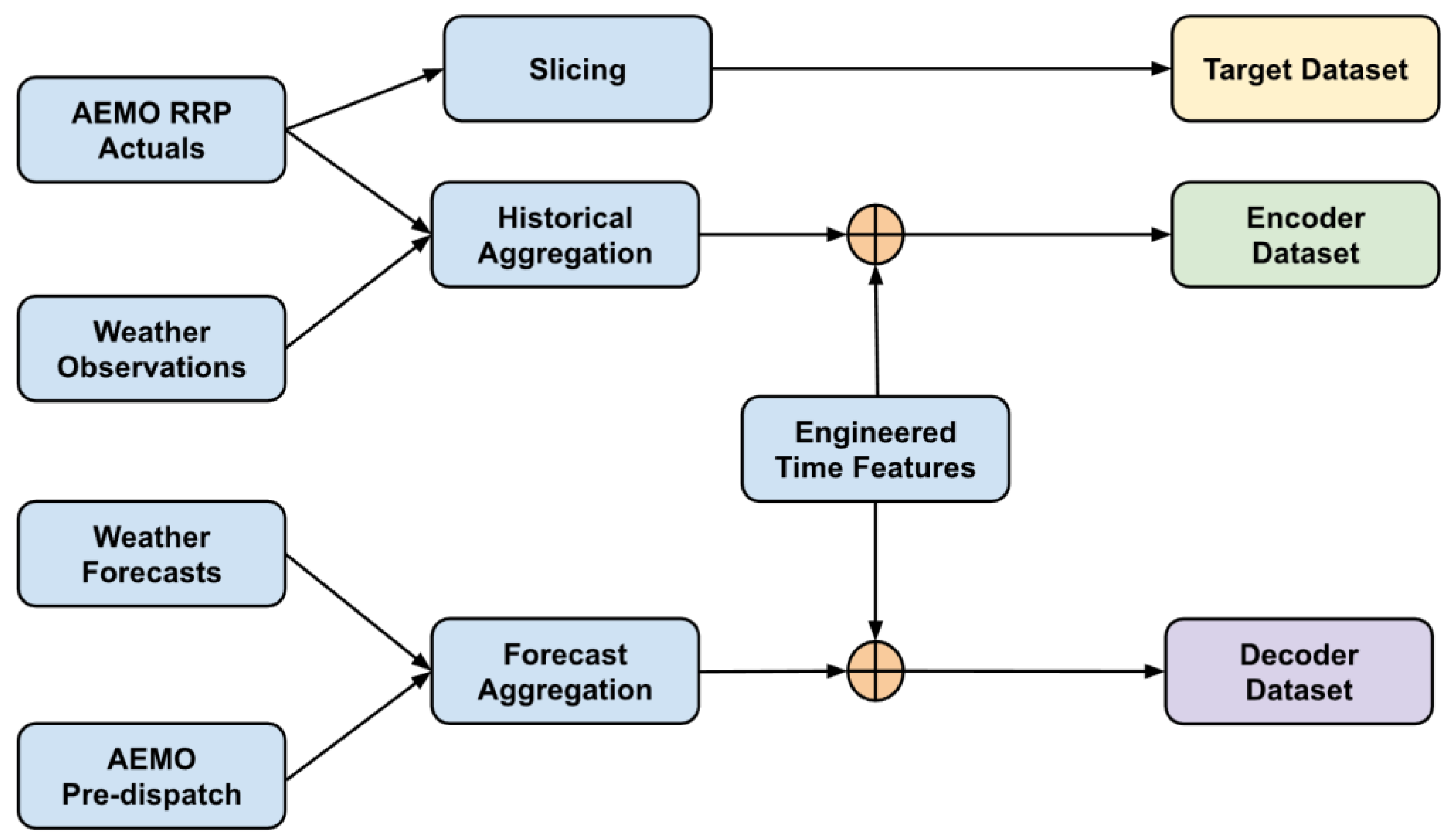
Figure 3.
Pre-layer normalisation encoder–decoder transformer architecture with parallel decoding. The encoder (left, purple box) processes historical inputs using multi-head self-attention and a position-wise feed-forward network, each wrapped with residual connections and layer normalisation (“Norm.”) applied before each block. The decoder (right, green box) processes known future inputs using self-attention and cross-attention over the encoder output, followed by a feed-forward layer. Predictions are produced via a final normalisation and linear projection layer. Positional encodings are added to both historical and future inputs. Parallel decoding is implemented as a non-autoregressive procedure in which the decoder generates all forecast horizons in parallel within one forward computation, eliminating the need to condition each timestep on earlier model outputs.
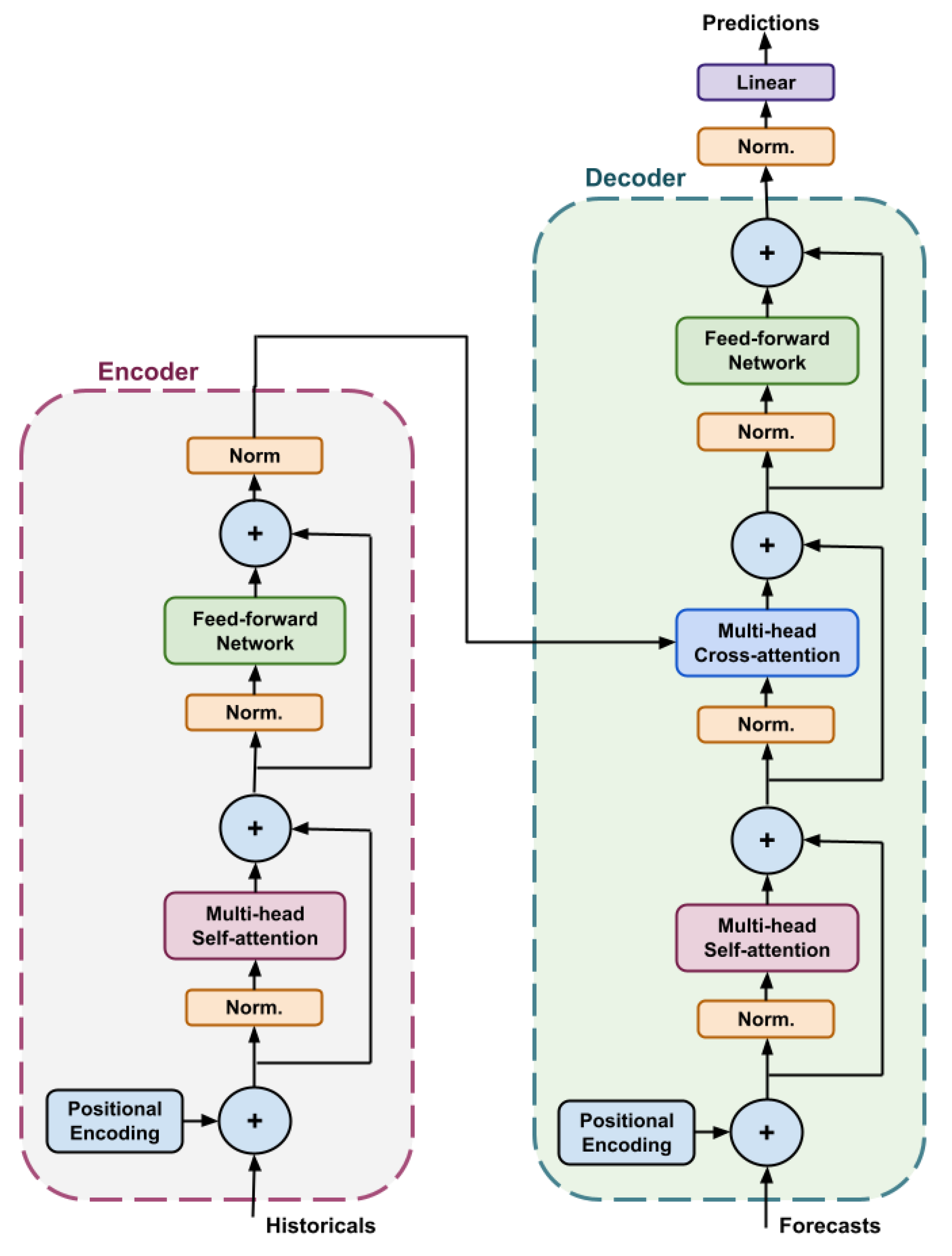
Figure 4.
Transformer architectures evaluated. (a) Enc-dec transformer with parallel decoding, (b) Enc-dec transformer with autoregressive decoding, (c) Encoder-only transformer, (d) Decoder-only transformer with parallel decoding, and (e) Decoder-only transformer with autoregressive decoding.
Figure 4.
Transformer architectures evaluated. (a) Enc-dec transformer with parallel decoding, (b) Enc-dec transformer with autoregressive decoding, (c) Encoder-only transformer, (d) Decoder-only transformer with parallel decoding, and (e) Decoder-only transformer with autoregressive decoding.
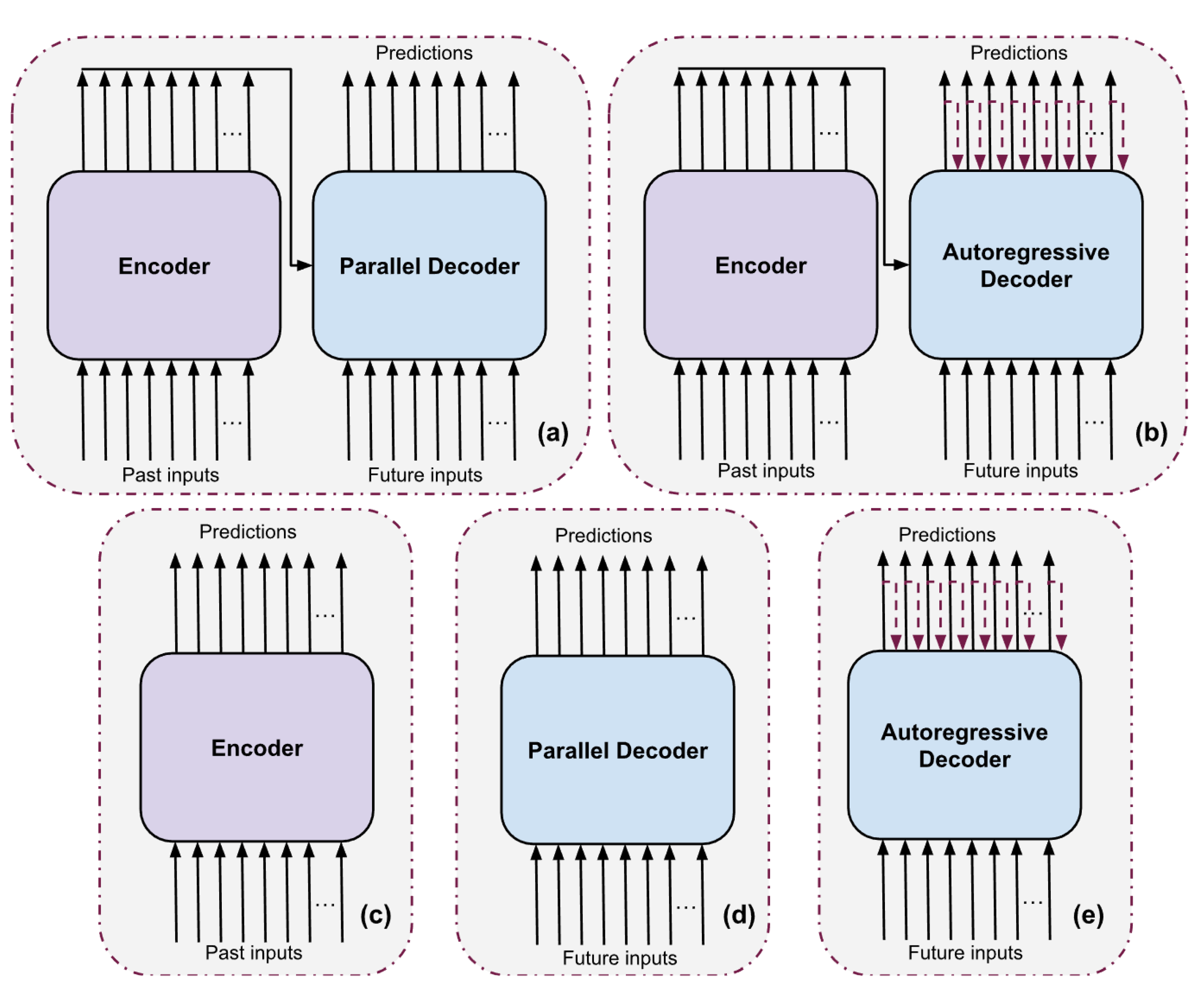
Figure 5.
Architectural overview of the comparison models used in this study, including a two-layer Long Short Term Memory network, the Temporal Fusion Transformer, TimesFM, and PatchTST. Each model represents a distinct class of sequence modelling approaches ranging from recurrent neural networks to attention based encoder architectures. These diagrams illustrate the structural differences in how each model processes historical inputs and generates multi step forecasts, providing context for the comparative evaluation presented in this work.
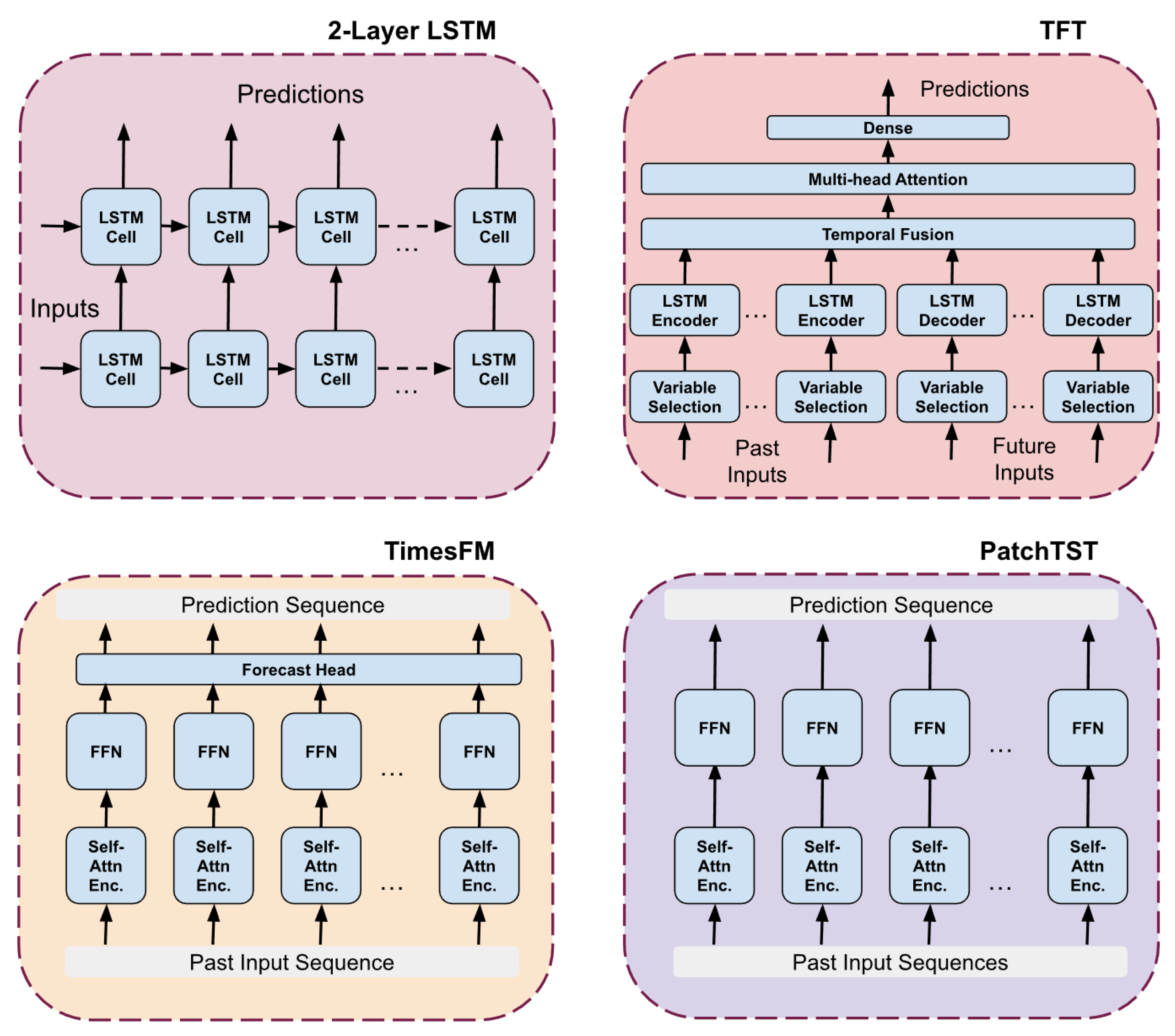
Figure 6.
NSW1 normalised MAPE performance of the top six models showing the parallel decoder-only transformer, the enc-dec transformer, and the temporal fusion transformer with the best performance across all prediction horizons.
Figure 6.
NSW1 normalised MAPE performance of the top six models showing the parallel decoder-only transformer, the enc-dec transformer, and the temporal fusion transformer with the best performance across all prediction horizons.
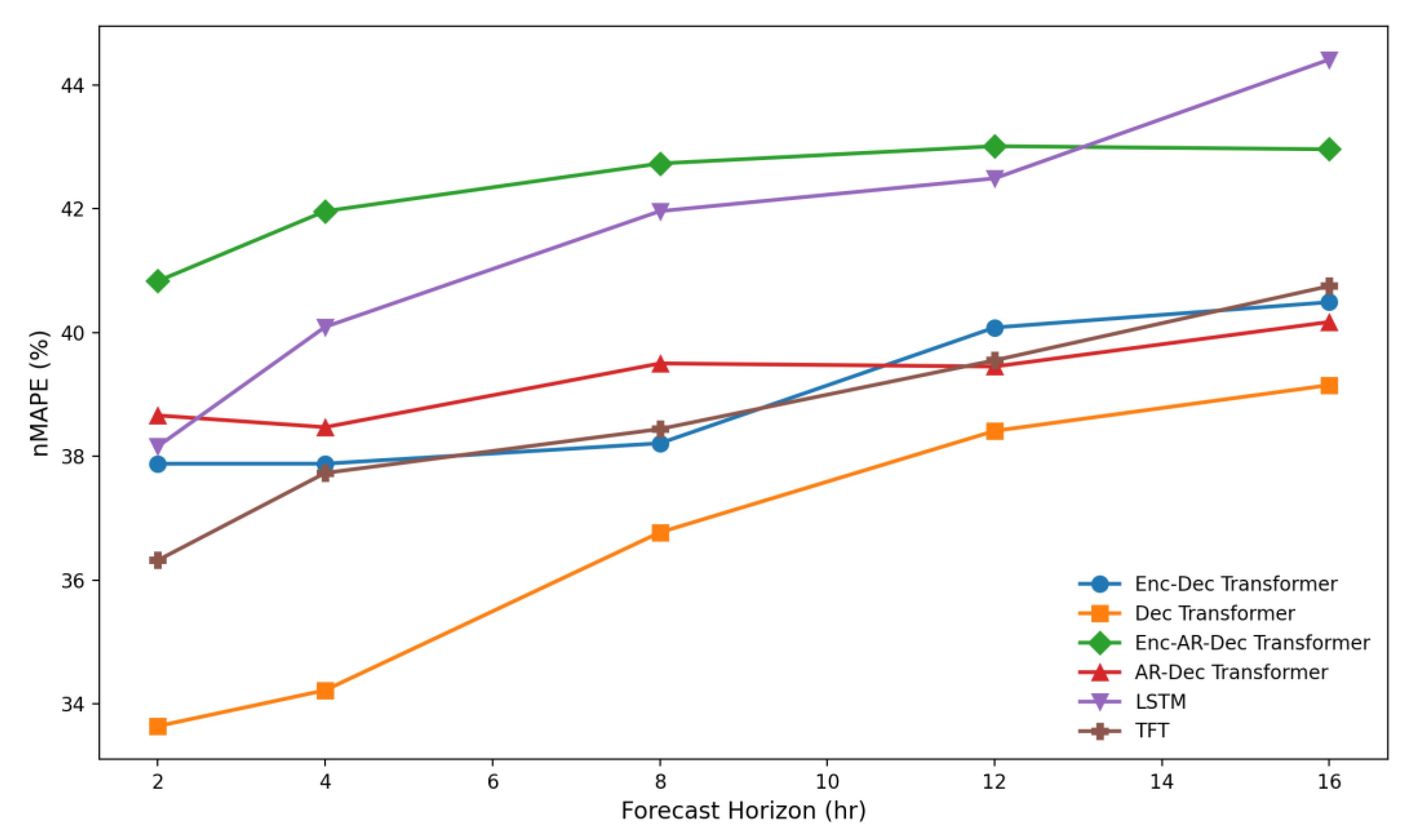
Figure 7.
Mean Absolute Error (MAE) distribution of all models for NSW1 across the full evaluation period. Violin plots illustrate both the spread and central tendency of errors for each architecture, highlighting the superior accuracy and lower variability of the transformer-based models compared with LSTM, TFT, PatchTST, TimesFM, and the official NEM forecasts. The plot shows that the encoder–decoder and decoder-only transformer variants consistently achieved the lowest MAE values, while TimesFM exhibited substantially higher error dispersion.
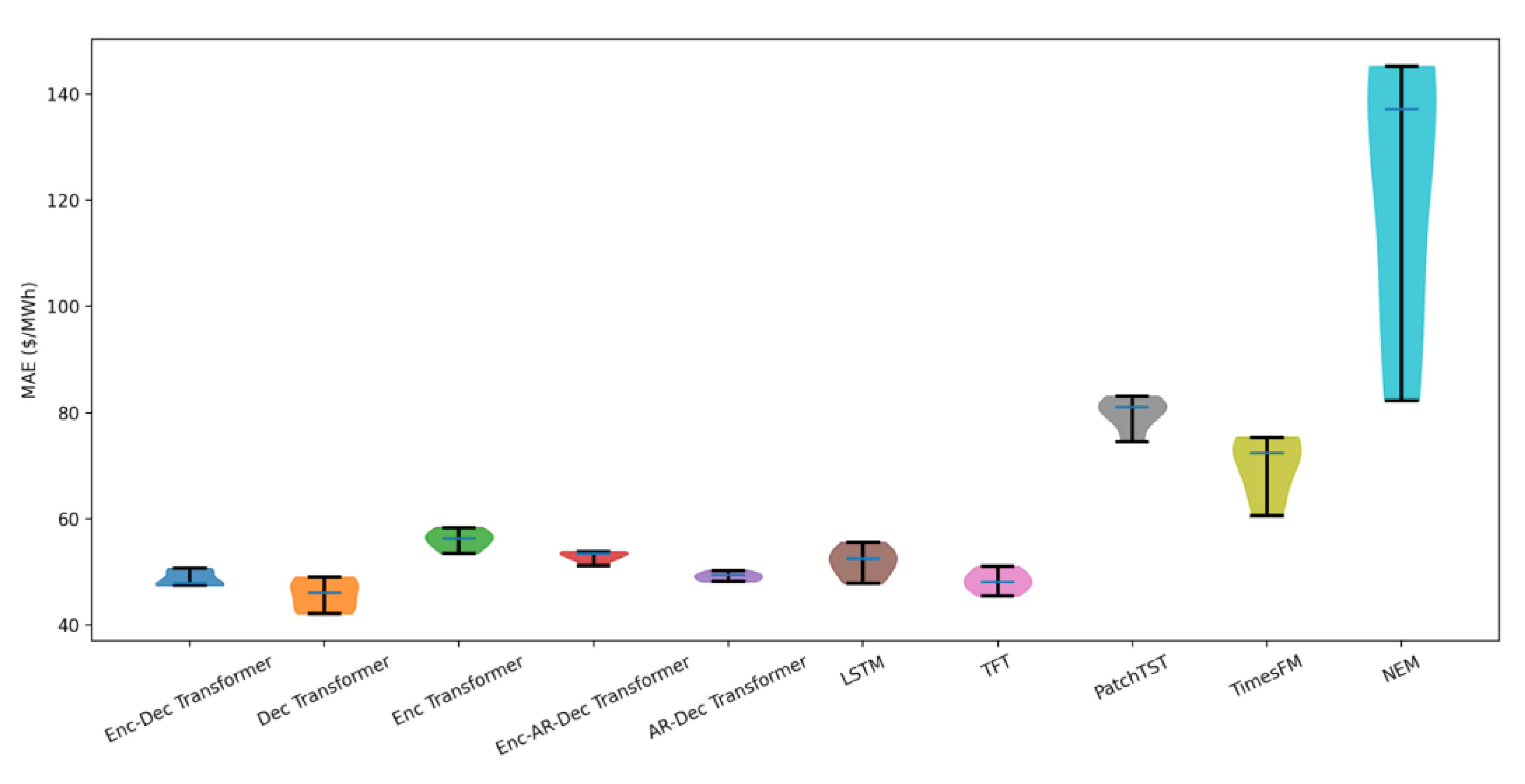
Figure 8.
NSW1 SHAP feature importance for the encoder and decoder features of the NSW1 transformer model. The results show that future-facing covariates—particularly the AEMO forecast price (F_RRP_NSW1) and regional predispatch demand and RRP forecasts—dominate model importance, accounting for the majority of predictive power. Historical signals and cyclical encodings contribute comparatively little.
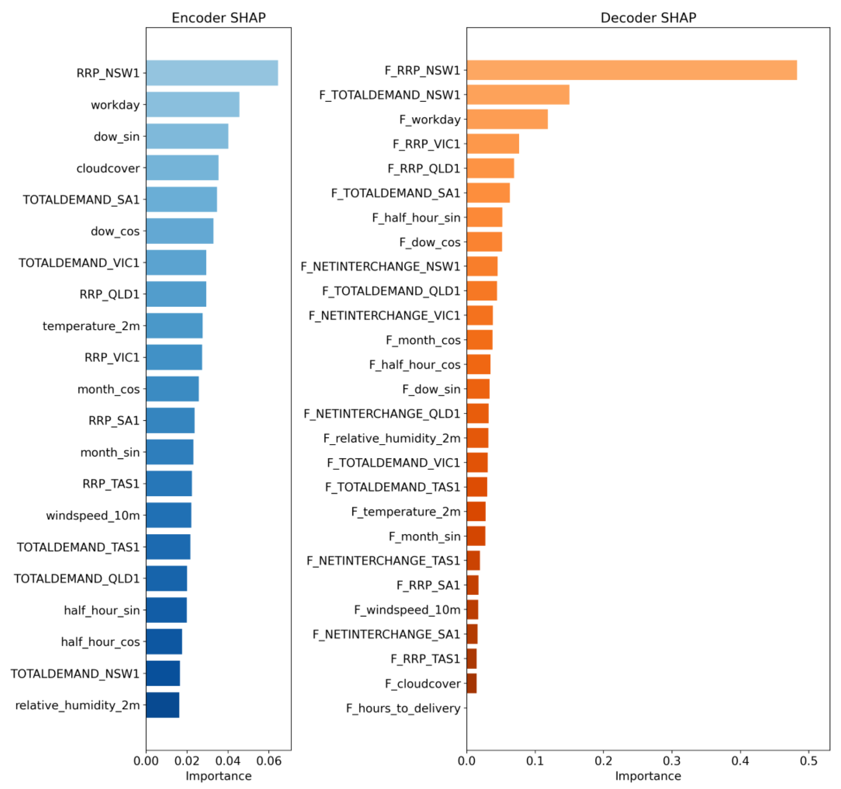
Figure 9.
QLD1 normalised MAPE performance of the top six models showing the parallel decoder-only transformer, enc-dec transformer, and the auto-regressive transformers with the best performance across all prediction horizons.
Figure 9.
QLD1 normalised MAPE performance of the top six models showing the parallel decoder-only transformer, enc-dec transformer, and the auto-regressive transformers with the best performance across all prediction horizons.
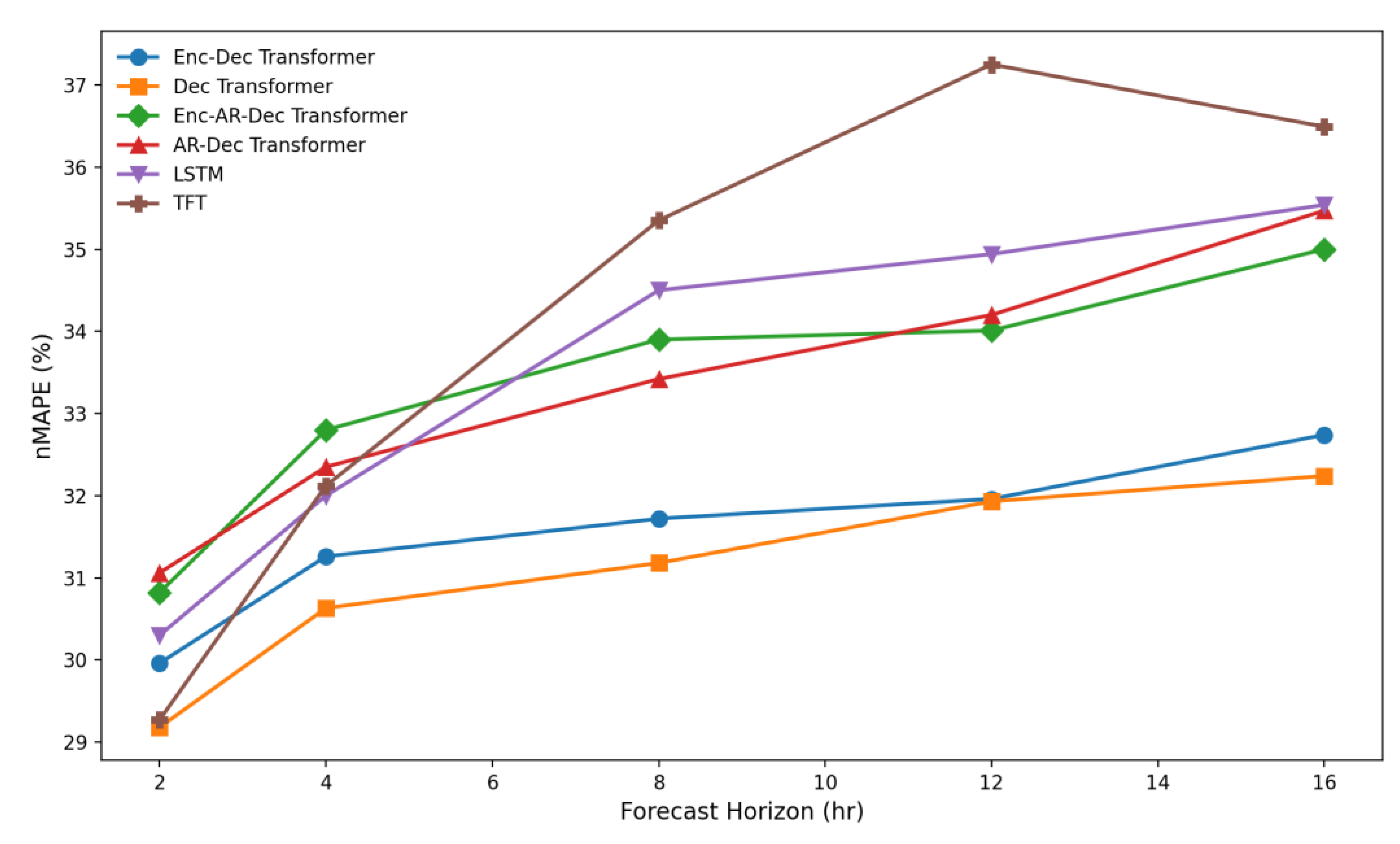
Figure 10.
VIC1 normalised MAPE performance of the top six models showing the temporal fusion transformer (TFT), enc-dec transformer and the parallel decoder-only transformer with the best performance across all prediction horizons.
Figure 10.
VIC1 normalised MAPE performance of the top six models showing the temporal fusion transformer (TFT), enc-dec transformer and the parallel decoder-only transformer with the best performance across all prediction horizons.

Figure 11.
Zoomed scatter plots of predictions vs true values for the models across all horizons in the NSW1 region. Extreme price spikes have been truncated. The plots illustrate the distribution of errors across various price ranges, with models showing a wide variance, especially with respect to price predictions above $400 with most models reverting to the mean for such rare events.
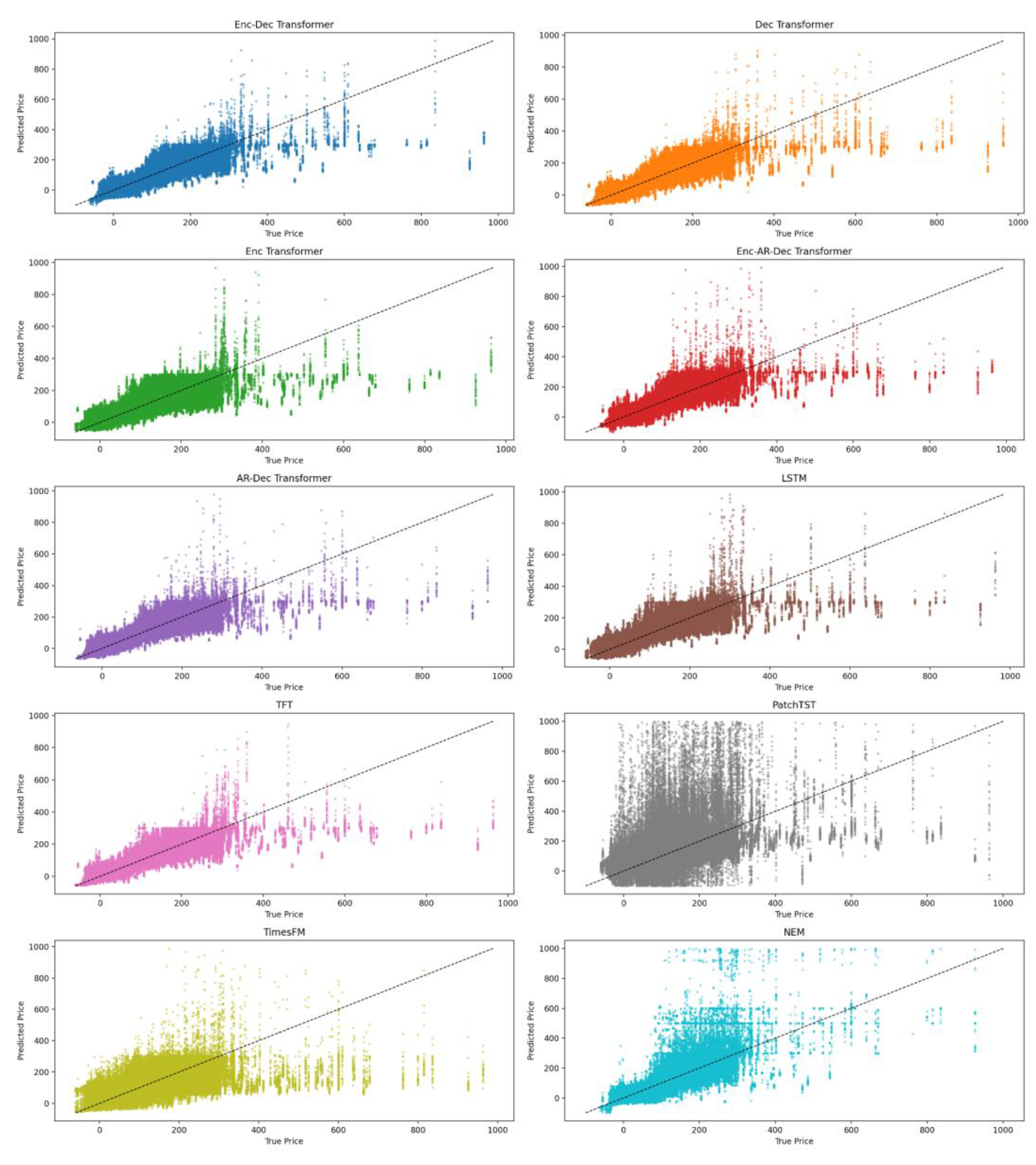
Table 1.
Summary of all input features used in this study, indicating whether each variable was incorporated as a historical encoder feature, a forecast decoder feature, or both. Data sources and brief descriptions are provided for clarity.
Table 1.
Summary of all input features used in this study, indicating whether each variable was incorporated as a historical encoder feature, a forecast decoder feature, or both. Data sources and brief descriptions are provided for clarity.
| Feature | Historical | Forecast | Data Source | Description |
| RRP | Yes | Yes | AEMO | Regional reference price for each NEM region |
| Demand | Yes | Yes | AEMO | Total demand for each NEM region |
| Net Interchange | Yes | Yes | AEMO | The amount of energy flowing in or out of each NEM region |
| Temperature, cloud cover, humidity, wind speed | Yes | Yes | Open Meteo | The more applicable weather conditions for the capital city of the given NEM region |
| Workday | Yes | Yes | Engineered | Binary indicating if the day of week is a workday |
| Half-hour Cos/Sin | Yes | Yes | Engineered | Circular encoded half-hour time slot to indicate diurnal position |
| Day of Week Cos/Sin | Yes | Yes | Engineered | Circular encoded day of the week to indicate weekly position |
| Month Cos/Sin | Yes | Yes | Engineered | Circular encoded month of the year to indicate yearly seasonal cycle |
| Hours to delivery | No | Yes | Engineered | Hours until the forecast point |
Table 2.
Summary of transformer model variants evaluated in this study, including tiny, small, medium, large, encoder-only, and decoder-only configurations. ‘layers’ refers to the number of repeated layers of the encoder and decoder; ‘heads’ represent the number of self-attention heads that each attention block has; ‘in+out’ refers to the input and output sequence lengths; ‘d_model’ is the main embedding size of the layers of model, ff_dim is the hidden layer size of the feed-forward network and dropout is the value used at each of the dropout layers.
| Model | layers | heads | in+out len | d_model | ff_dim | dropout |
| Tiny, enc-dec | 2 | 2 | 96+32 | 64 | 256 | 0.05 |
| Small, enc-dec | 3 | 4 | 96+32 | 128 | 512 | 0.05 |
| Med, enc-dec | 3 | 4 | 96+32 | 256 | 1024 | 0.05 |
| Large, enc-dec | 4 | 8 | 96+32 | 512 | 2048 | 0.05 |
| Small, decoder only | 3 | 4 | 0+32 | 128 | 512 | 0.05 |
| Small, encoder only | 3 | 4 | 96+0 | 128 | 512 | 0.05 |
Table 3.
Hyperparameters used for models in this study.
| Hyperparameter | Transformers & LSTM | TFT | PatchTST |
| Batch size | 128 | 128 | 128 |
| Input sequence length | 96 x 30-minute periods | 96 x 30-minute periods | 96 x 30-minute periods |
| Scaler | QuantileTransformer | QuantileTransformer | - |
| Output sequence length | 32 x 30m periods | 32 x 30m periods | 32 x 30m periods |
| Dropout | 0.05 | 0.10 | 0.10 |
| Initial learning rate | 2e-4 | 2e-4 | 1e-5 |
| Global Clipnorm | 2.0 | - | - |
| Optimiser | Adam (β=0.9, β2=0.999, ε=1e-9) | Adam | Adam (clipnorm=0.01) |
| Loss | Huber (δ=0.8) | Quantile[0.1,0.5,0.9] | MSE |
| Max. epochs | 20 | 20 | 20 |
| Reduce LR on Plateau | Factor=0.5, Patience=2 | Factor=0.5, Patience=2 | - |
| Early stop | Patience=5, Monitor=val_loss | Patience=5, Monitor=val_loss | - |
| Patch & Stride | - | - | 24 & 6 |
Table 4.
NSW1 region comparative model normalised MAPE (%) results. The table reports percentage errors at fixed forecast horizons (2, 4, 8, 12, and 16 hours ahead), enabling direct comparison of short-, medium-, and long-range predictive performance. The listed transformer models are all of the “small” size.
| Model | 2h | 4h | 8h | 12h | 16h |
| Enc-Dec Transformer | 37.9 | 37.9 | 38.2 | 40.1 | 40.5 |
| Dec Transformer | 33.6 | 34.2 | 36.8 | 38.4 | 39.2 |
| Enc Transformer | 42.7 | 44.0 | 45.0 | 45.6 | 46.6 |
| Enc-AR-Dec Transformer | 40.8 | 42.0 | 42.7 | 43.0 | 43.0 |
| AR-Dec Transformer | 38.7 | 38.5 | 39.5 | 39.5 | 40.2 |
| LSTM | 38.2 | 40.1 | 42.0 | 42.5 | 44.4 |
| TFT | 36.3 | 37.7 | 38.4 | 39.5 | 40.8 |
| PatchTST | 59.4 | 64.7 | 66.4 | 65.0 | 63.6 |
| TimesFM | 48.3 | 53.3 | 59.4 | 60.2 | 57.8 |
| NEM | 65.6 | 82.7 | 116.0 | 109.6 | 114.6 |
Table 5.
QLD1 NEM region results for all small-model architectures, showing normalised MAPE across 2-, 4-, 8-, 12-, and 16-hour forecast horizons. All models were fully retrained on QLD1 targets using the same input features and training configuration as the NSW1 experiments.
Table 5.
QLD1 NEM region results for all small-model architectures, showing normalised MAPE across 2-, 4-, 8-, 12-, and 16-hour forecast horizons. All models were fully retrained on QLD1 targets using the same input features and training configuration as the NSW1 experiments.
| Model | 2h | 4h | 8h | 12h | 16h |
| Enc-Dec Transformer | 30.0 | 31.3 | 31.7 | 32.0 | 32.7 |
| Dec Transformer | 29.2 | 30.6 | 31.2 | 31.9 | 32.2 |
| Enc Transformer | 42.2 | 43.6 | 45.3 | 45.0 | 45.1 |
| Enc-AR-Dec Transformer | 30.8 | 32.8 | 33.9 | 34.0 | 35.0 |
| AR-Dec Transformer | 31.1 | 32.3 | 33.4 | 34.2 | 35.5 |
| LSTM | 30.3 | 32.0 | 34.5 | 34.9 | 35.5 |
| TFT | 29.3 | 32.1 | 35.3 | 37.2 | 36.5 |
| PatchTST | 60.3 | 77.5 | 97.6 | 94.3 | 99.0 |
| TimesFM | 62.1 | 82.5 | 104.3 | 99.0 | 105.6 |
| NEM | 57.0 | 79.1 | 120.4 | 124.7 | 121.9 |
Table 6.
VIC1 NEM region results for all small-model architectures, showing normalised MAPE across 2-, 4-, 8-, 12-, and 16-hour forecast horizons. Each model was retrained on VIC1 targets to evaluate performance consistency and model robustness across different NEM regions.
Table 6.
VIC1 NEM region results for all small-model architectures, showing normalised MAPE across 2-, 4-, 8-, 12-, and 16-hour forecast horizons. Each model was retrained on VIC1 targets to evaluate performance consistency and model robustness across different NEM regions.
| Model | 2h | 4h | 8h | 12h | 16h |
| Enc-Dec Transformer | 38.0 | 38.8 | 39.2 | 40.5 | 41.3 |
| Dec Transformer | 37.3 | 38.9 | 40.3 | 40.8 | 41.7 |
| Enc Transformer | 61.3 | 63.0 | 64.7 | 64.7 | 65.4 |
| Enc-AR-Dec Transformer | 38.7 | 41.4 | 43.2 | 43.8 | 46.0 |
| AR-Dec Transformer | 38.9 | 39.9 | 41.4 | 43.0 | 45.9 |
| LSTM | 39.7 | 42.1 | 44.1 | 44.8 | 45.2 |
| TFT | 36.3 | 37.7 | 37.7 | 39.6 | 39.6 |
| PatchTST | 82.9 | 95.1 | 105.1 | 101.6 | 107.7 |
| TimesFM | 85.2 | 100.3 | 112.3 | 107.2 | 114.5 |
| NEM | 35.7 | 41.0 | 60.3 | 59.3 | 61.4 |
Table 7.
NSW1 model-size comparison for the encoder–decoder transformer, showing normalised MAPE across 2-, 4-, 8-, 12-, and 16-hour horizons. Results indicate that the small model provides a good balance between accuracy and capacity for this dataset.
Table 7.
NSW1 model-size comparison for the encoder–decoder transformer, showing normalised MAPE across 2-, 4-, 8-, 12-, and 16-hour horizons. Results indicate that the small model provides a good balance between accuracy and capacity for this dataset.
`1 Encoder-decoder transformer model sizes are defined in Section 2.3.
Table 8.
Diebold-Mariano test results comparing each model’s forecasts with the official NEM forecasts for the NSW1 region. All models show statistically significant improvements over the NEM benchmark at the 95% confidence level.
Table 8.
Diebold-Mariano test results comparing each model’s forecasts with the official NEM forecasts for the NSW1 region. All models show statistically significant improvements over the NEM benchmark at the 95% confidence level.
| Model | Diebold Mariano-stat | p-value |
| Enc-Dec Transformer | -6.85 | 7.6e-12 |
| Dec Transformer | -7.13 | 1.1e-12 |
| Enc Transformer | -6.27 | 7.1e-10 |
| Enc-AR-Dec Transformer | -6.52 | 7.5e-11 |
| AR-Dec Transformer | -6.84 | 8.6e-12 |
| LSTM | -6.57 | 5.4e-11 |
| TFT | -6.90 | 5.6e-12 |
| PatchTST | -4.03 | 5.6e-5 |
| TimesFM | -4.92 | 9.0e-7 |
Disclaimer/Publisher’s Note: The statements, opinions and data contained in all publications are solely those of the individual author(s) and contributor(s) and not of MDPI and/or the editor(s). MDPI and/or the editor(s) disclaim responsibility for any injury to people or property resulting from any ideas, methods, instructions or products referred to in the content. |
© 2025 by the authors. Licensee MDPI, Basel, Switzerland. This article is an open access article distributed under the terms and conditions of the Creative Commons Attribution (CC BY) license (http://creativecommons.org/licenses/by/4.0/).
Copyright: This open access article is published under a Creative Commons CC BY 4.0 license, which permit the free download, distribution, and reuse, provided that the author and preprint are cited in any reuse.


