
Submitted:
09 December 2025
Posted:
10 December 2025
You are already at the latest version
Abstract
Background: In Japan, the number of older adults living alone has been increasing, raising the risk of unnoticed health decline or solitary death. Continuous monitoring using sensors can help detect behavioral changes indicating health issues and has the potential to support both older adults and their families.
Methods: We obtained behavior and temperature data, continuously recorded over a long period at 15-min intervals from sensors installed in the homes of nine older adults living alone. After data cleaning, behavioral signals were analyzed using Fourier spectral analysis and multiple regression to extract 13-dimensional behavioral feature vectors. We attempted to detect temporal changes and behavioral characteristics by whitening these data and performing correspondence analysis.
Results: Spectral analysis revealed 24-hour periodicity in all users’ behavior. Based on changes in the maximum component value and adjusted R2, individuals were classified into a stable group (SG) and a fluctuating group (FG). Boundary variance and false error analyses confirmed that behavioral temporal changes and individual characteristics could be detected objectively.
Conclusions: The findings showed that temporal changes in daily behavior among older adults living alone can be detected using simple continuous sensor data, suggesting potential for early detection of health-related changes and preventive support in home.
Keywords:
sensors
; older adults
; living alone
; monitoring system
; behavioral change
; temporal change
; preventive support
1. Introduction
Japan leads the world in the pace of its aging population. The proportion of older adults living alone is increasing, and solitary deaths among them have increased by 34% from 20 years ago [1]. Similarly, aging populations are increasing in other countries, and the ability to watch over older adults living alone is crucial in giving them and their families peace of mind. Monitoring systems can detect both falls and reduced activity levels, which indicate declining health. In recent years, numerous monitoring systems for older adults based on information and communication technology and sensing technology have been deployed [2,3], and seasonal variations and periodicity in elderly behavior have already been identified [4,5]. Some studies have equipped older adults with wearable devices to detect and recognize activities of daily living [6]. Other studies have inferred activity patterns by monitoring the usage of lifelines such as gas and water [7]. However, such studies are invasive for older adults and are only short term. Such studies aim to observe and detect interruptions in the activities of the older adults, such as when gas or water was "not used". The purpose of this study was to detect changes in the behavioral patterns of older adults living alone over time. Changes in behavioral patterns over time indicate that something has happened or is about to happen; for example, the onset of dementia or a precursor to a stroke. If we can capture such changes, we can consider responses such as taking them to a medical facility or arranging for them to live with someone before an incident occurs. Thus, this research has the potential to support the lives of older adults living alone and their families. We analyzed long-term data collected from non-invasive movement and temperature sensors installed in the residences of older adults living alone. The results reveal that it is possible to capture temporal changes in the behavioral patterns of older adults from these data with our original methods.
2. Materials and Methods
2.1. Datasets Collection
We acquired data collected continuously by sensor devices manufactured by Japan Aito System Co., Ltd. (each housing unit contains two sensors) [8]. The devices were already in use in the homes of the 14 users who comprised the initial study population.
Pyroelectric Infrared(IR)Sensor: This detects human (or animal) movement within a range of 5 m and records the number of movements detected every 15 min. The sensors were installed only in households without pets (14 users).
Temperature Sensor: The indoor temperature in °C was recorded as the average over 15 min.
The devices were installed in only one location—the living room, bedroom, kitchen, or other area most frequently visited by users. The devices automatically sent the data to a database server via the Internet every 15 min.
Note that the monitoring system from Aito System Limited, which generated the data used in this study, was already in actual use within households, independent of our study. In addition, this data was acquired through an extremely simple mechanism: only the number of sensor responses within a fixed time period and the average temperature within that same period were automatically transmitted. Therefore, the data contained some rough elements, such as missing values.
2.2. Datasets Cleaning
The sensor datasets contained only the measurement date, time, IR data, and temperature. To impute missing values, we performed the following processes.
- The total number of complete datasets in 1 day (24 h) is 4 × 24 = 96. Therefore, we deleted days with fewer than or more than 96 datasets.
- When datasets were deleted in step 1, we simply connected the data from the preceding and following days.
- Including users with numerous deleted datasets in the analysis significantly lowers the analytical accuracy. Therefore, we excluded users with >10% deleted data.
2.3. Ethical Consideration
We received data from Aito in the form of CSV files. The sensor data were managed separately from users’ personal information and background details by Aito. Thus, the datasets lacked any personal details.
Minimum background information (age, gender, family composition, care level, residential style, and comorbidity) was provided separately from the sensor data by Aito.
During sensor device installation, Aito explained the provision of data to third parties for research purposes and obtained opt-in consent from each user.
2.4. Analytical Methods
2.4.1. Temporal Changes in Activity
To investigate what could be revealed from the raw sensor data, we examined temporal changes in activity. To indicate activity, we used the number of responses per 15 min (the "signal") from the IR sensor. We calculated the daily average values of both the signal and the temperature sensor measurements and presented them in a time series.
2.4.2. Spectral Analysis of All Signals
We analyzed the periodicity of activity by data processing and spectral analysis of all signals per user. First, the initial data points (where total data count, for maximum N) were extracted from each signal data set.
Next, we defined each data segment as , and set , where is the mean. This set the constant of the Fourier series to 0. Subsequently, a Fast Fourier Transform (FFT) was executed on to obtain the power spectrum (spectral density) and autocorrelation function [9].
2.4.3. Analysis of Behavioral Characteristics and Temporal Changes
The long-term spectral analysis of the signal data in section 2.4.2 revealed a 24-h cycle in each signal. To identify behavioral characteristics and temporal changes in them, we created "characteristic vectors" and "benchmark data" using the signal data as described next.
Characteristic Vector
To investigate data with a 24-h (daily) cycle, we segmented the signal data into 11-day intervals, as detecting a cycle requires an observation period of at least five times the target cycle length [10]. In this study, considering ten times the length of a day, we segmented the data into 11-day intervals. Each 11-day segment contains 96 × 11 = 1,056 data. For the dataset (data group), we calculated the following.
The spectrum of a periodic function with period T has peaks at frequencies . In the overall spectrum in Section 2.4.2, the spectral peak at frequencies of (corresponding to ) was small. So, we assumed prediction equation (1) for the original dataset using trigonometric functions of these 12 frequencies.
We conducted multiple regression analysis using equation (1) for each dataset, calculating the coefficients , , and the adjusted coefficient of determination R squared (hereafter, ). Then, from the obtained , , we calculated 12 spectra .
These spectra characterize the periodicity of the signal. We combined these 12 spectra with the values from the regression analysis to form a 13-dimensional column vector (where denotes the transpose matrix). We designated this as the characteristic vector for the respective dataset.
Generally, the in multiple regression analysis is considered to indicate the degree to which the results of the equation explain the variance of the dependent variable. Here, let "" represent the integral value around the 12 periodic peaks in the signal spectrum. Let "" represent the integral value of the entire spectrum. Call the ratio of to () "". and have a strong positive correlation [refer to Appendix A].
That is, a large indicates that spectral components other than the 12 peaks are small. We included in the characteristic vector as an indicator of the strength of periodicity in the signal. Furthermore, was used independently of as an indicator of the strength of periodicity in the signal.
Benchmark Data
We selected 20 consecutive vectors as benchmark data from the set of characteristic vectors. For whitening processing (described in next section "Whitening of Benchmark Data"), the number of data must be greater than or equal to the dimension of the covariance matrix (13 in this case). The choice of benchmark data was based on the purpose of comparison. For example, when the purpose was to investigate a user’s temporal variation, we selected 20 characteristic vectors as "benchmark data" from the first 220 days of that user’s signal data. We compared the benchmark data with other characteristic vectors. The relationship between the characteristic vectors and the benchmark data is shown in Figure 1. To eliminate differences in scale and correlations between vector components when comparing the benchmark data with other characteristic vectors, we whitened the benchmark data and transformed the characteristic vectors other than the benchmark data.
Whitening of Benchmark Data
Each component of the characteristic vector follows an approximately normal distribution within each user’s data [Appendix B]. Then, we conducted the following whitening processing (decorrelation and normalization of each component data) on the benchmark data [11,12].
Data Decorrelation: Let the 20 characteristic vectors in the benchmark data be . The mean vector of was defined as , the variance vector as , and the covariance between i and j as follows.
Using these, the following covariance matrix was created.
This is a symmetric matrix. Therefore, we find the eigenvalues of and the corresponding eigenvectors of length 1, defining the matrix S as follows:
Then:
Applying a linear transformation to the vector using the transpose matrix of matrix S causes the transformed data to become uncorrelated. That is:
At this point, data with different components of become uncorrelated.
Data Standardization: Find the mean and variance for each component of :
where:
Standardize using this mean and variance :
This makes each vector component follow a standard normal distribution with mean 0 and variance 1.
Transformation of Non-benchmark Data (Correspondence Transformation)
For data other than the benchmark data, each characteristic vector was transformed using the matrix S obtained in the whitening process of the benchmark data and then standardized using the mean and variance derived from the benchmark data.
Specifically, the following was performed on the target characteristic vector to create a characteristic vector in comparison with the benchmark data.
This process is referred to as the "correspondence transformation" applied to the characteristic vector. Unless otherwise specified, the benchmark data undergo whitening, and other characteristic vectors undergo the correspondence transformation.
Comparing Two Data Sets
The means of all components of the characteristic vector for the whitened benchmark data are 0, and their variances are 1. We introduce boundary variance V as a criterion for recognizing the difference between the set of characteristic vectors containing this whitened benchmark data ("SA") and the set of characteristic vectors that have undergone correspondence transformation without the benchmark data ("SB").
Defining the boundary variance as V, if the maximum value of any component in a characteristic vector (from SA or SB) is , that vector is judged to belong to SA. If it is , it is judged not to belong to SA (i.e., different from SA) (Figure 2).
Here, two types of misclassifications can occur. One is when the maximum value of the characteristic vector components taken from SA is . In this case, the data are judged not to be SA (but to be SB). This is a misclassification where data that is from SA is judged as SB. The other is when the maximum value of the characteristic vector components taken from SB is . In this case, it is a misclassification, where data from SB are judged as SA. Therefore, we define the false error rates for these data sets as the following two types [13,14].
(False Reject Rate):
The proportion of data included in SA that is judged as belonging to SB, defined as (the number of characteristic vectors in SA where the maximum value of components ) ÷ (the total number of characteristic vectors in SA).
(False Accept Rate):
The proportion of data belonging to set SB that is incorrectly judged as belonging to SA, defined as (the number of characteristic vectors in SB where the maximum value of components ) ÷ (the total number of characteristic vectors in SB).
3. Results
3.1. Result 1: Temporal Change in Activity
Figure 3 shows the temporal change in activity (average daily signal count) of User C. The change in signal over time showed decreased activity during summer, when room temperature rose and increased activity during the winter. This pattern was common among all 9 users, though the magnitude of the signal differed.
3.2. Result 2: Signal spectral analysis
User C’s data acquisition period was the longest (Table 1). Thus, we report the analysis results for User C’s signal spectrum (Figure 4). Results were similar for others.
Figure 4 shows relatively large, sharp peaks at representing the period. These large peaks all correspond to integer divisions of a 24-h (1-day) period. This confirms that the signal data exhibits a primary 24-h cycle. Beyond a cycle of or a frequency of , these peaks diminish and become indistinguishable from other peaks not related to the 24-h cycle.
Several peaks indicate cycles other than 24-h. These peaks were of the size of the 24-h peak. Among them, the main ones were days (likely corresponding to yearly) and days (weekly). All had small peak values and were ignored in subsequent analyses.
3.3. Result 3: Analysis of Behavioral Characteristics and Temporal Changes
The primary issue in this study is whether the analysis can identify each user’s behavioral patterns, can be defined as consistent signal patterns that persist over a fixed period.
First, we investigated whether there is a fixed pattern that persists for a certain period in the signal. If such a signal pattern continues for a fixed duration, then there is likely a fixed behavioral pattern present. We used the first 20 characteristic vectors as benchmark data. We whitened the benchmark data, and for the other characteristic vectors, we conducted corresponding transformations. Figure 5 shows the time-series plots of the maximum value of each user’s characteristic vector components ("") and the change in .
The of all users remained around 2 between times 0 and . After , it exceeded this and fluctuated uniquely among users. In particular, the of users C, E, F, H, and I (the "stable group": SG) fluctuated stably around 5, and a consistent pattern appeared to persist. Conversely, other users had large fluctuations (A, B, D, G; the "fluctuating group": FG). variation over time fluctuated greatly, and their behavior did not appear to follow a consistent pattern.
Of the five members of the SG, of three was around 0.2, and that of only 1 (User C) was . Of the four members of the FG, except for Use D, remained for extended periods. R2 is an indicator of periodicity, with signifying that the signal exhibits nearly periodic fluctuations [Appendix A]. indicates a state of very low periodicity. The tendency for to be smaller in the SG suggests that data periodicity is lower in the SG.
3.4. Result 4: Recognition of Differences in Behavioral Patterns
Result 3 reveals that the maximum values of the characteristic vector components of some users varied little, suggesting that these users maintain consistent behavioral patterns.
So we investigated whether our method could identify differences in these behavioral patterns. To do so, we selected data where patterns are presumed to differ. It is reasonable to assume that different users have different behavioral patterns. Therefore, we investigated whether the analysis could distinguish differences in behavioral patterns between users in SG (with low variation in s). We denoted the set of characteristic vectors of one user as SA and that of another user as SB. One of the 20 consecutive characteristic vectors in set SA was selected as the benchmark data, which was then whitened and transformed. Using the boundary variance described in section 2.4.3, we conducted the classification between SA and SB and measured the FRR and FAR misclassification rates.
Figure 6 illustrates how the misclassification rates between each user and other users in the SG change when the boundary variance is varied.
In the SG, classification was generally possible with boundary variance V values between 4 and 6. This is the boundary variance that minimizes the total misclassification rate of SA and SB (i.e., the sum of SA’s and SB’s ). The average boundary variance where was minimized was 5.75, and a false recognition rate () was 0.35 at that point. The fact that user classification is possible using boundary variance values indicates a high potential for recognizing changes in behavioral patterns using our method.
3.5. Result 5: Temporal Changes in Behavioral Patterns
Result 4 showed that the boundary variance V for identification is between 4 and 6. This corresponds to the maximum value of the characteristic vector components in the SG being around 5. This indicates that as long as the maximum vector component values are concentrated around 5.0, the user’s behavior pattern has not changed. This finding also corresponds to the maximum value of components exceeding 10 in the FG over time. We investigated this point in more detail for each user.
To examine the extent of changes over time for each user, the following analysis was conducted. First, we define groups of 20 characteristic vectors arranged in the user’s time series as analytical data. The first analytical data within this group is designated as the benchmark data. That is, the time series is grouped every (220 days), and comparisons were made between each set of data. We whitened the benchmark data and conducted a correspondence transformation on the characteristic vectors within the analytical data. We plotted the for each user’s benchmark data and for each analytical data by time. Specifically, for the benchmark data and each analytical data, we calculated the rate of characteristic vectors whose maximum component value exceeded V.
Figure 7 shows the for the five users in the SG group, which exhibited low variation, and Figure 8 shows the for the four users in the FG group, which exhibited high variation. In each figure, the horizontal axis represents the boundary variance V, and the vertical axis represents the misclassification rate () of the benchmark data and of each other time point’s analytical data. In both figures, the greater the deviation of the at times other than the benchmark data from the benchmark data’s (i.e., the greater the lateral spread from the line of benchmark data), the more it indicates a change in behavioral patterns at that time.
Figure 8 clearly shows greater spread from the line of benchmark data than Figure 7. In Figure 7, the range was 8 to 10, peaking at 16, with no significant overtime spread. In contrast, in Figure 8, the for all users except User A exceeded 16, and a significant expansion of the over time was evident. This indicates that users in Figure 8 showed greater changes in their behavioral patterns than those in Figure 7 over time.
Therefore, it can be concluded that behavioral changes occur when the expands to 10 or higher. According to this criterion, the behavior of the FG (User A, B, D, G) changed over time, as predicted in Result 3.
Note that we had no detailed information on individual clinical aspects and home environments of the users in this study, so little can be inferred from differences in behavioral patterns among them. However, within the scope of available information, we will discuss the relationship between the temporal changes in behavior observed in the FG and the clinical and home-related information.
The of User A increased toward the end of the data collection period (Figure 5). As we later learned that A had moved from living alone into a care home, the change in behavior suggests that a behavioral abnormality may have occurred before admission. User B showed a major change in behavioral patterns around (30 × 11 = 330 days). The reason is unknown, but since User B continued living alone even after this change, it may not have been a long-term problem. The maximum value of User D increased significantly around (550 days). User D is known to have dementia and depression. It is possible that her cognitive function changed around this time. User G showed significant fluctuations immediately after the benchmark data period (), and this state persisted. User G has a medical history of Hypertension, Rheumatism, and MCI (Mild Cognitive Impairment). For instance, it is possible that User G developed MCI with behavioral changes after the benchmark data period, and this condition continued until the end.
4. Discussion
The purpose of this paper was to capture temporal changes in the behavior of elderly individuals using a monitoring system. The data used was continuous behavioral data acquired in natural settings.
Time-series analysis of the raw data revealed seasonal changes in signal and patterns (decreased activity in summer, increased activity in winter). Cepeda et al. (2018) investigated activity levels by having 3,507 participants wear accelerometers and found the opposite: physical activity levels were higher in summer than in winter [5], as found in other studies too [16,17]. Several factors may explain why our results show the opposite: we focused on older adults living alone; Japanese summers are hot and humid; and data collection methods differed. More work is needed to clarify the differences.
Spectral analysis of the signal data indicates a 24-hour cycle in the signal, i.e., activity levels. The presence of a 24-hour cycle (circadian rhythm) in human activity has already been demonstrated in numerous previous studies [18,19].
To investigate whether temporal variations in behavior could be detected from signal data, we conducted multiple regression analysis using predictive models. The 12 calculated spectral components (behavioral features) and the adjusted (an indicator of periodicity) were combined and used as a behavioral characteristic vector. This revealed that the characteristic vectors could distinguish between users. This means that the behavioral characteristics of each user can be extracted. If we can demonstrate differences in characteristic vectors of a user over time, we can detect temporal variations in that user’s behavioral patterns.
As a result, the temporal change in behavior differed between users, dividing them into two groups. One group, SG, showed small changes and stability, while the other group, FG, exhibited significant fluctuations starting at a certain point. We demonstrated that for users belonging to the SG, we could classify characteristics of behavioral patterns distinct from those of other users. Moreover, in the FG, we were able to distinguish differences in behavioral patterns over time within the same user, that is, the temporal change in behavior.
Therefore, the analysis method presented in this paper successfully captured the differences in behavioral characteristics and temporal changes among elderly individuals living alone, even when using large amounts of continuous signal data obtained from a simple system.
Numerous studies have been conducted on developing systems to monitor the behavior of older adults using data acquired from sensors or on tracking their activities [6,7]. Ioan et al. (2019) installed sensors in all rooms occupied by older adult subjects, mapped their response frequencies, and used image recognition techniques to investigate deviations and tendencies toward deviation from their daily activity routines [20]. Dorsaf Z. et al. (2020) proposed a framework for detecting changes in the daily activities of older adults. They stated that using this framework enables the detection not only of sudden changes, such as falls or temporary illnesses, but also of "silent changes" occurring over long periods [21]. This focus on detecting "silent changes" is similar to our objective. However, they collected data labeled by multiple sensors in a smart home—such as sleep, meals, outings, and toilet use—as signal data, and used a normal behavior model based on data collected over only 1 month, unlike our study [21].
Ohta S. et al. (2002) installed sensors in six rooms of a house and conducted an activity monitoring study using infrared sensors for a total of 80 months (maximum 20 months) with eight older adults [22]. This study attempted to estimate health status by comparing dwell times in specific rooms (e.g., toilet) with records. However, it differs from our study in its sensor complexity and its use of dynamic programming (DP) matching to distinguish between normal and abnormal activity.
Serge H. et al. (2009) attempted to classify the activities of daily living (ADL) of older adults with a history of stroke using electromyography (EMG) and accelerometers [23]. They reported that the classification method achieved sensitivity and specificity of over 95%. However, they noted that it remains unclear whether this method would function effectively on data collected from unrestricted daily activities outside of an experimental setting [23].
This study has novelty in that it uses data naturally obtained from the daily lives of older adults living alone, rather than experimental data, as had been a concern by Serge H. et al. (2009) [23]. Also, significant importance lies in the fact that behavioral characteristics and temporal change can be detected from the very simple continuous data used in this study. That is, the simple signal data analysis method we presented has the potential to lead to a wide range of support applications. This includes not only monitoring changes in the activities of older adults living alone but also observing changes in the activities of people with behavioral disorders living at home and children.
In the future, we need to conduct the verification of the temporal change in behavioral patterns detected in this analysis with the medical time-series progression information regarding the users. While we were able to detect behavioral characteristics and temporal change in this study, we could not detect characteristics inherent in the data, such as signs of stroke or dementia. Detecting these inherent characteristics could lead to support for older adults living alone and their families.
5. Patents
Author Contributions
Conceptualization, M.H. and Y.T.; methodology, Y.T. and M.H.; software, Y.T.; investigation and analysis M.H. and Y.T.; validation, Y.T.; data curation, M.H.; writing—original draft preparation, M.H. and Y.T.; writing—review and editing, Y.T. and M.H.; visualization, M.H. and Y.T.; All authors have read and agreed to the published version of the manuscript.
Funding
This research received no external funding.
Institutional Review Board Statement
Not applicable.
Informed Consent Statement
Not applicable.
Data Availability Statement
Restrictions apply to the availability of these data. Data were obtained from Aito System Co., Ltd. and are available from the authors with the permission of Aito System Co., Ltd..
Acknowledgments
The authors would like to express their sincere gratitude to Aito System Co., Ltd. for kindly providing the data used in this study. The authors also wish to extend their heartfelt appreciation to Dr. Takashi Tahara for his valuable advice regarding the structure, data analysis methods, and discussion of this manuscript.
Conflicts of Interest
The authors declare no conflicts of interest.
Abbreviations
The following abbreviations are used in this manuscript:
| NC | Not Care Needed |
| LA | Living Alone |
| WF | With Familiy |
| MCI | Mild Cognitive Impairment |
| FFT | Fast Fourier Transform |
| R2 | R squared |
| PI | Periodicity Indicator |
| FRR | False Reject Rate |
| FAR | False Accept Rate |
| MCV | Maximum value of each user’s Characteristic Vector |
| SG | Stable Group |
| FG | Fluctuatin Group |
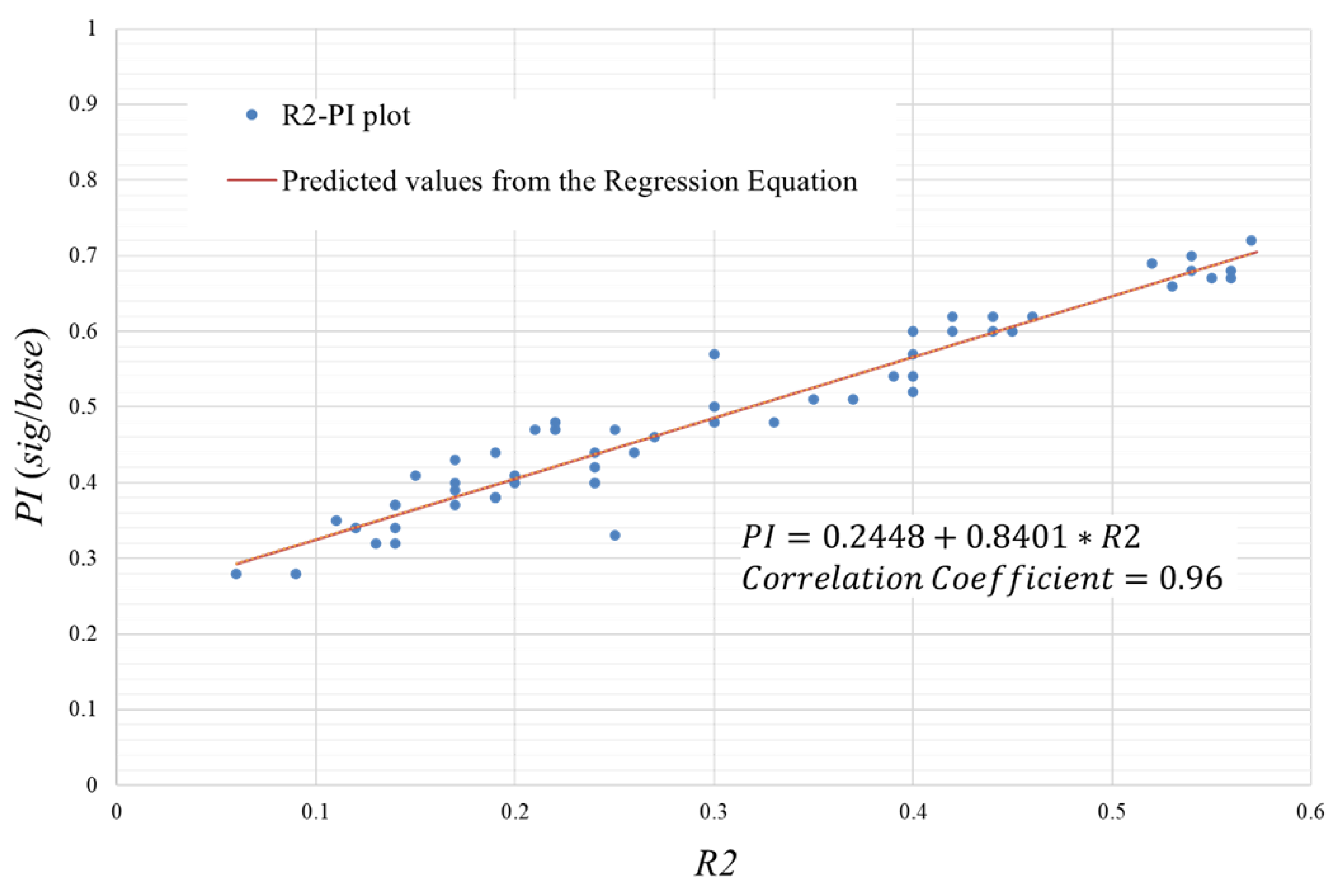
Appendix A. Relationship between Periodicity Indicators and R2
As shown in Methods 2.4.3. of the main text, the spectrum of the signal data peaks at frequencies . Therefore, as a periodicity indicator, we calculated the ratio of the integral of the spectrum within before and after this peak frequency to the integral of the background spectrum. Let be the spectrum and f be the frequency .
We define the periodicity indicator (Periodicity Indicator) as:
When has a peak only at and is 0 elsewhere, . Furthermore, when is white noise:
Therefore:
From the above, . As periodicity strengthens, approaches 1.0, allowing periodicity to be determined by the value. The results of correlating this and using the signal data are shown in Figure A1.
The relationship between and is shown by the regression line , where corresponds to . That is, the range of is 0 to 0.95. Therefore, since and are strongly correlated, we can use as a substitute for .
Figure A1.
Correlation between and .
Appendix B. Test for Normality
For each component of the 20 feature vectors of each analysis dataset, we examined whether its distribution was non-normal by means of the Kolmogorov–Smirnov test. We concluded that the components of the feature vector for all analysis datasets appear normal (the probability of error in claiming a non-normal distribution is ).
The raw data for this analysis consisted of 96-dimensional vectors of signal data. None of the components of these vectors followed a normal distribution. Consequently, analytical methods such as whitening could not be applied when using these components directly. One reason for using the periodic components extracted via Fourier analysis that they followed a normal distribution.
References
- Nomura, M.; McLean, S.; Miyamori, D.; Kakiuchi, Y.; Ikegaya, H. Isolation and unnatural death of elderly people in the aging Japanese society. Science & Justice 2016, 56(2), 80–83. [Google Scholar] [CrossRef] [PubMed]
- Casanova-Perez, R. A.; Padilla-Huamaninco, P. G.; Freitas-Vidal, C. I. D.; Choi, Y. K. Home Behavior Monitoring Module in OpenEMR: Use of home sensors as Patient-Generated Data (PGD) for elderly care. Journal AMIA Annu Symp Proc. 2018, 2279–2283. [Google Scholar]
- Pol, M.; van Nes, F.; van Hartingsveldt, M.; Buurman, B.; de Rooij, S.; Kröse, B. Older People’s Perspectives Regarding the Use of Sensor Monitoring in Their Home. Journal Gerontologist 2016, 56, 485–493. [Google Scholar] [CrossRef] [PubMed]
- Sayegh, S.; Van Der Walt, M.; Al-Kuwari, M. G. One-year assessment of physical activity level in adult Qatari females: a pedometer-based longitudinal study. Journal Int J Womens Health 2016, 8, 287–293. [Google Scholar] [CrossRef] [PubMed]
- Cepeda, M.; Koolhaas, C. M.; van Rooij, F. J. A.; Tiemeier, H.; Guxens, M.; Franco, O. H.; Schoufour, J. D. Seasonality of physical activity, sedentary behavior, and sleep in a middle-aged and elderly population: The Rotterdam study. Maturitas 2018, 110, 41–50. [Google Scholar] [CrossRef] [PubMed]
- Mathunjwa, B. M.; Chen, Y.-F.; Tsai, T.-C.; Hsu, Y.-L. A Lifestyle Monitoring System for Older Adults Living Independently Using Low-Resolution Smart Meter Data. Sensors 2024, 24, 3662. [Google Scholar] [CrossRef] [PubMed]
- Koketsu, T.; Ohno, Y.; Ishihara, T.; Nishimoto, Y.; Kobayashi, K. Monitoring Living Activities of the Elderly Living Alone Using a Lifeline. Japanese Journal of Applied IT 2018, 3, 12–19. [Google Scholar]
- Aito System Ltd. Available online: https://aitosys.com/aishiru/ (accessed on 24 November 2025).
- Cooley, J. W.; Tukey, J. W. An Algorithm for the Machine Calculation of Complex Fourier Series. Mathematics of Computation 1965, 19, 297–301. [Google Scholar] [CrossRef]
- Mourão, M.; Satin, L; Schnell, S. An Algorithm for the Machine Calculation of Complex Fourier Series. Mathematics of Computation 1965, 19(90), 297–301. [Google Scholar] [CrossRef]
- Christopher, B.; Michael, J.; Jon, K.; Bernhard, S. Pattern Recognition and Machine Learning. In Information Science and Statistics; Springer New York: New York, USA, 2006; pp. 565–570. [Google Scholar]
- Hyvärinen, A.; Oja, E. Independent Component Analysis: Algorithms and Applications. Neural Networks 2000, 13, 411–430. [Google Scholar] [CrossRef] [PubMed]
- Jain, A. K.; Ross, A. A.; Nandakumar, K. Introduction to Biometrics, Foreword by James Wayman; Springer New York: New York, USA, 2017; pp. 18–22. [Google Scholar]
- Dass, S.; Zhu, Y.; Jain, A. Validating a Biometric Authentication System: Sample Size Requirements. IEEE Transactions on Pattern Analysis and Machine Intelligence 2006, 28, 1902–319. [Google Scholar] [CrossRef] [PubMed]
- Overview of Japan’s Climate (Japan Meteorological Agency). Available online: https://www.data.jma.go.jp/gmd/cpd/longfcst/en/tourist_japan.html (accessed on 23 November 2025).
- Charles, E. M.; Patty, S. F.; James, R. H.; Edward, J. S.; Philip, A. M.; Milagros, C. R.; Cara, B. E.; Ira, S. O. Seasonal variation in household, occupational, and leisure time physical activity: longitudinal analyses from the seasonal variation of blood cholesterol study. Am J Epidemiol 2001, 153, 172–183. [Google Scholar]
- Ma, Y.; Olendzki, B. C.; Li, W.; Hafner, A. R.; Chiriboga, D.; Hebert, J. R.; Campbell, M.; Sarnie, M.; Ockene, I. S. Seasonal variation in food intake, physical activity, and body weight in a predominantly overweight population. Eur J Clin Nutr 2006, 60, 519–528. [Google Scholar] [CrossRef] [PubMed]
- Vitaterna, M. H.; Takahashi, J. S.; Turek, F. W. Overview of circadian rhythms. Alcohol Res Health 2001, 25, 85–93. [Google Scholar] [PubMed]
- Bass, J. Circadian topology of metabolism. Nature 2012, 491, 348–356. [Google Scholar] [CrossRef] [PubMed]
- Susnea, I.; Dumitriu, L.; Talmaciu, M.; Pecheanu, E.; Munteanu, D. Unobtrusive Monitoring the Daily Activity Routine of Elderly People Living Alone, with Low-Cost Binary Sensors. Sensors 2019, 19, 2264. [Google Scholar] [CrossRef] [PubMed]
- Zekri, D.; Delot, T.; Thilliez, M.; Lecomte, S.; Desertot, M. A Framework for Detecting and Analyzing Behavior Changes of Elderly People over Time Using Learning Techniques. Sensors 2020, 20, 7112. [Google Scholar] [CrossRef] [PubMed]
- Ohta, S.; Nakamoto, H.; Shinagawa, Y.; Tanikawa, T. A Health Monitoring System for Elderly People Living Alone. Journal of Telemedicine and Telecare 2002, 8, 151–156. [Google Scholar] [CrossRef] [PubMed]
- Roy, S. H.; Cheng, M. S.; Chang, S.-S.; Moore, J.; De Luca, G.; Nawab, S. H. Combined sEMG and Accelerometer System for Monitoring Functional Activity in Stroke. IEEE Transactions on Neural Systems and Rehabilitation Engineering 2009, 17, 585–594. [Google Scholar] [CrossRef] [PubMed]
Figure 1.
Relationship between the characteristic vectors and the benchmark data.
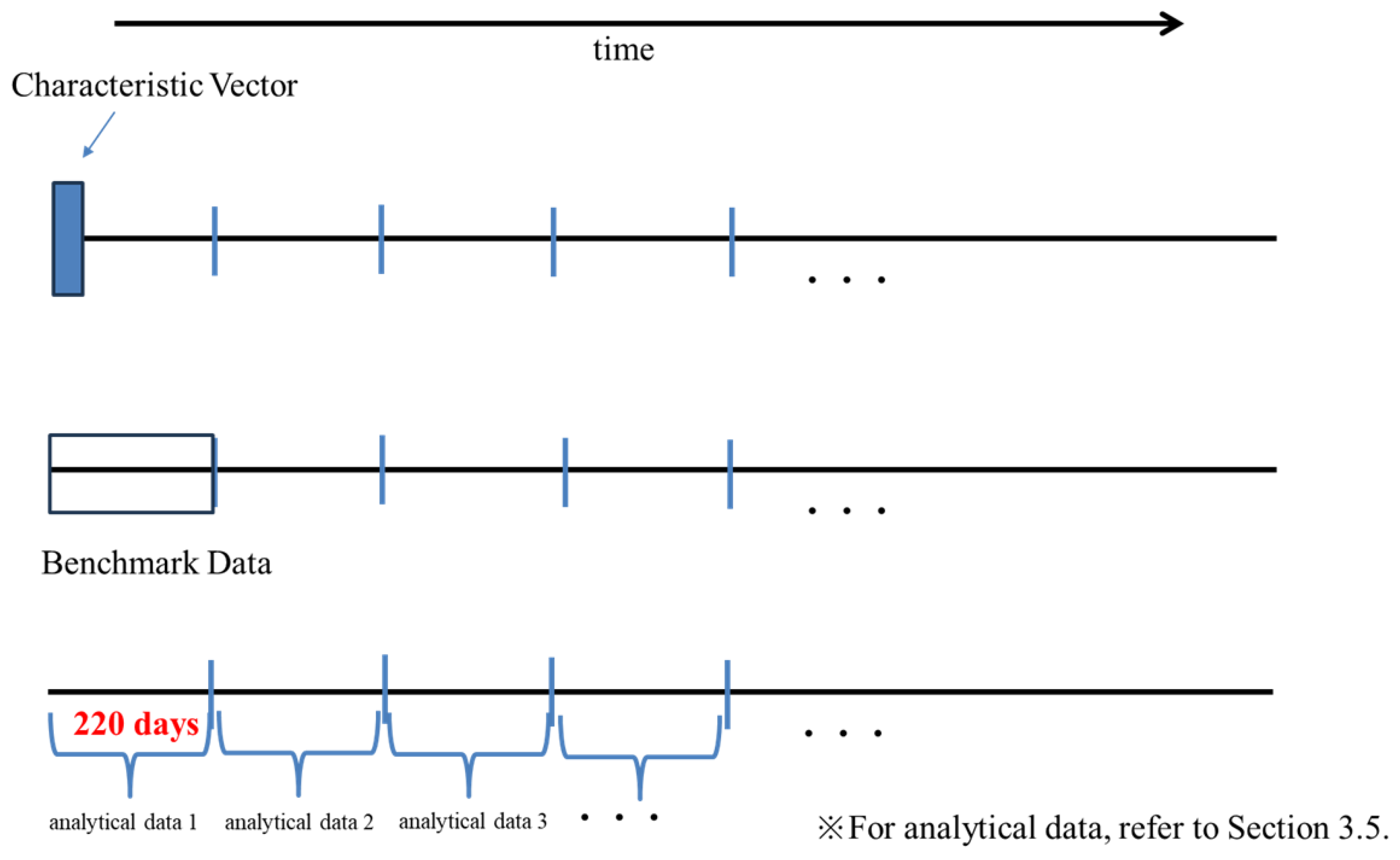
Figure 2.
Misclassification Rate by Boundary Variance V.
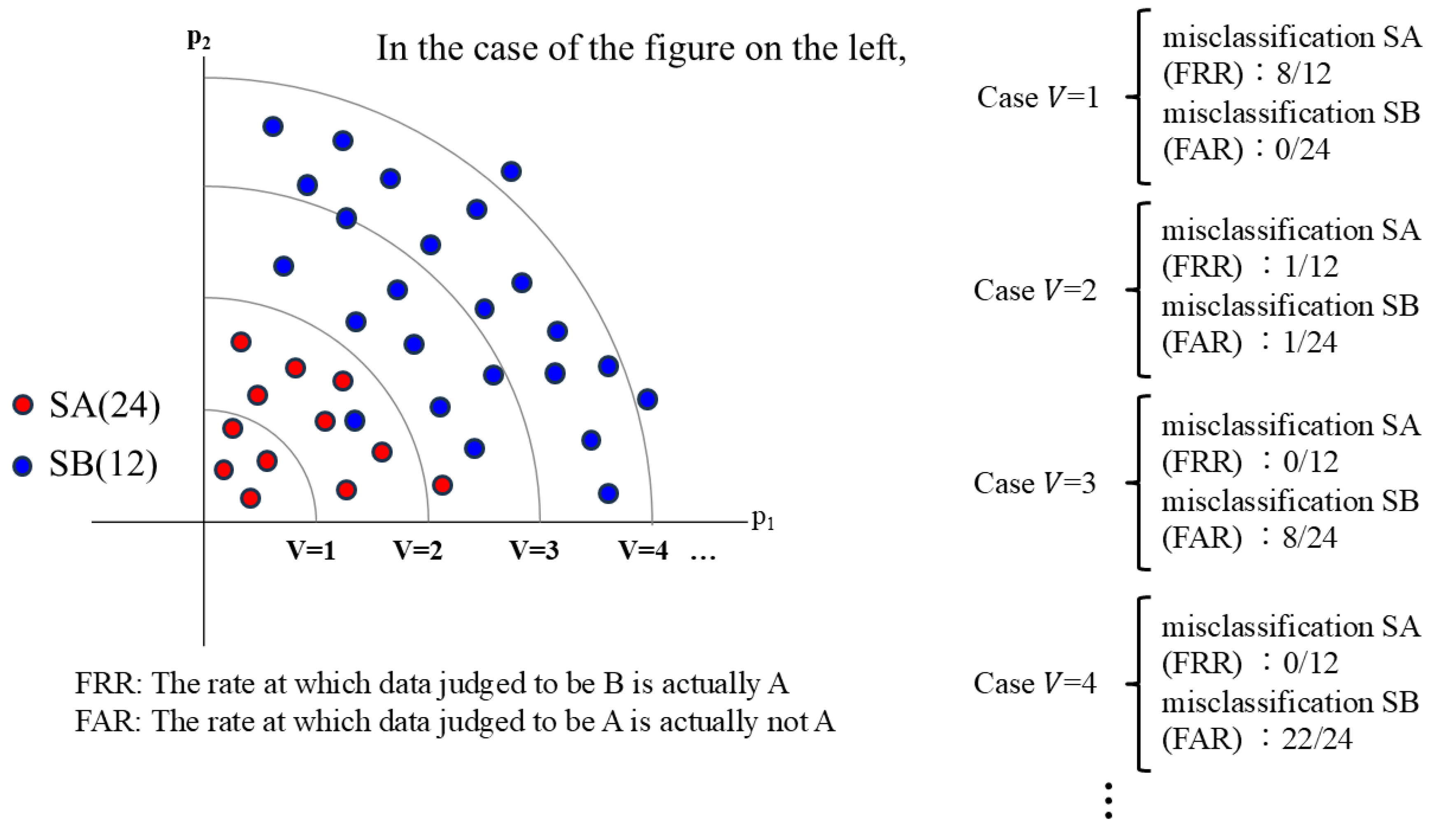
Figure 3.
Seasonal variation of signal and temperature. Orange line, average room temperature; blue line, average signal values. Yellow shading, summer; gray shading, winter. Seasonal divisions: spring (March – May), summer (June – August), autumn (September – November), winter (December – February) [15].
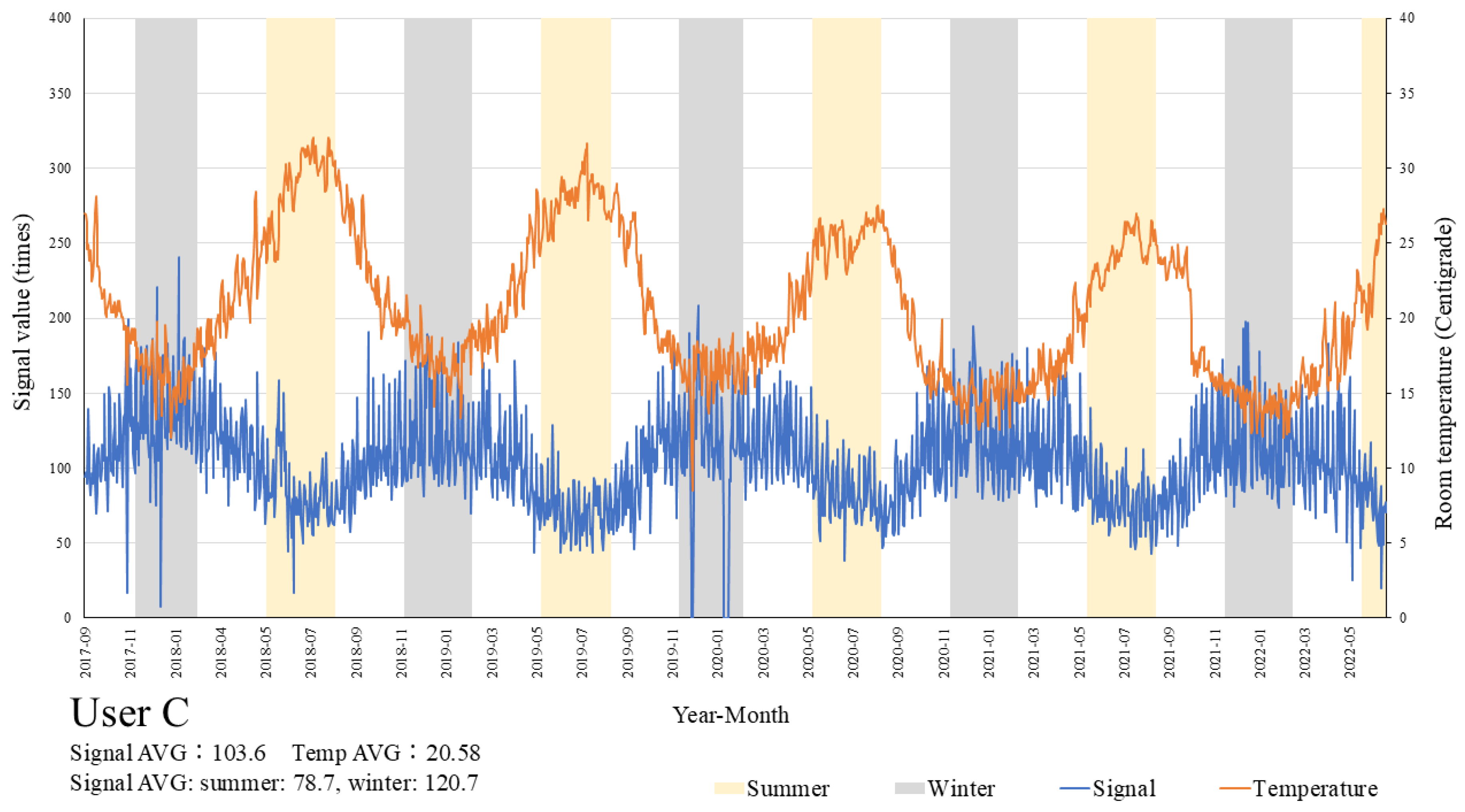
Figure 4.
The spectra of User C for the entire observation period (Frequency: 0.0-0.6).
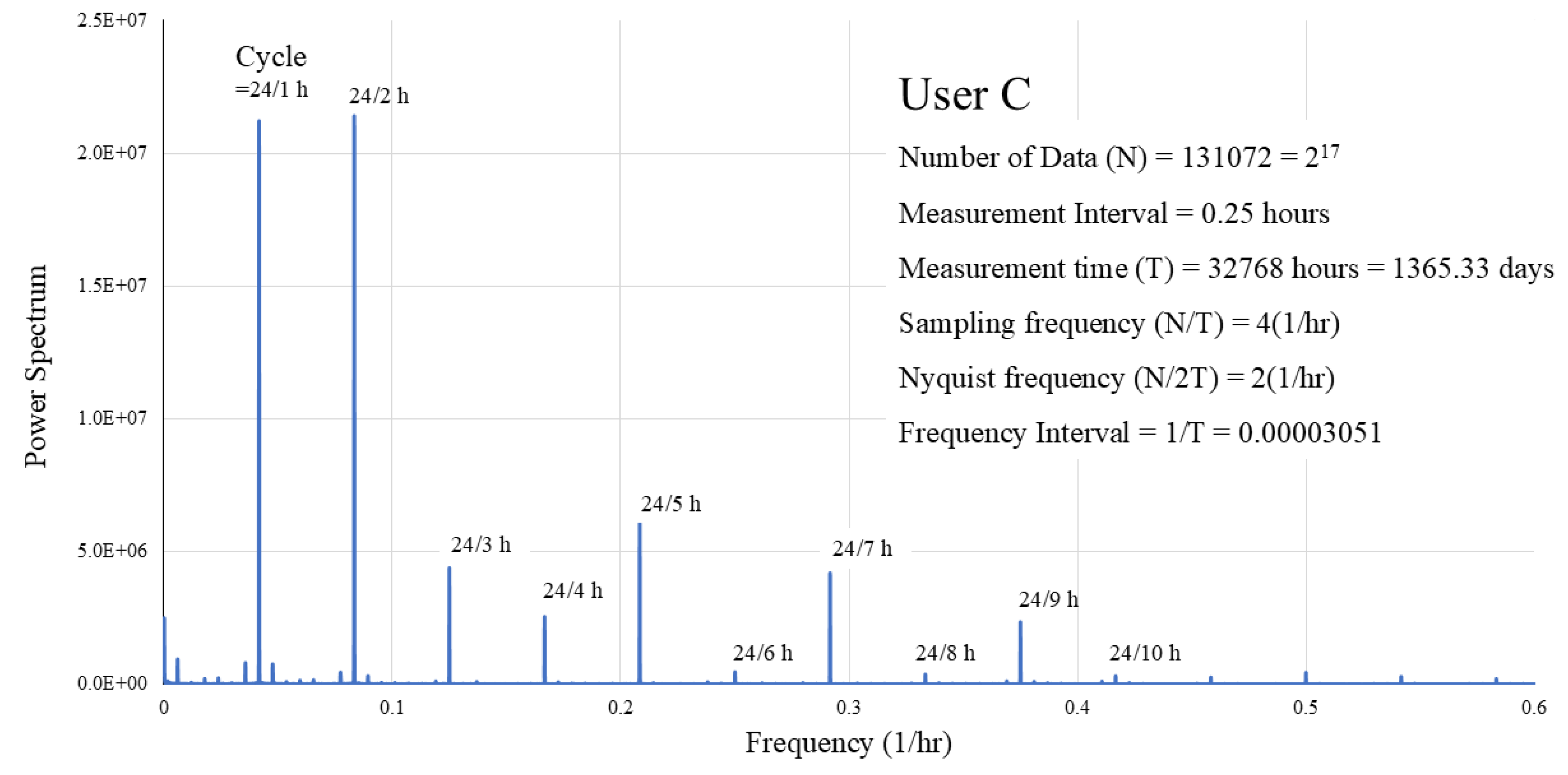
Figure 5.
Longitudinal changes in and . The maximum value on the horizontal axis was set to 120 (11 × 120 days = 1320 days = 3.6 years), and the maximum value on the vertical axis was set to 20. Although User G’s maximum value far exceeds 20, the graph was drawn with a maximum vertical value of 20 for comparison among all users. The horizontal axis represents time, measured in units (u) based on the 11 days of characteristic vector measurement period. The first (220 days) represents the benchmark data.
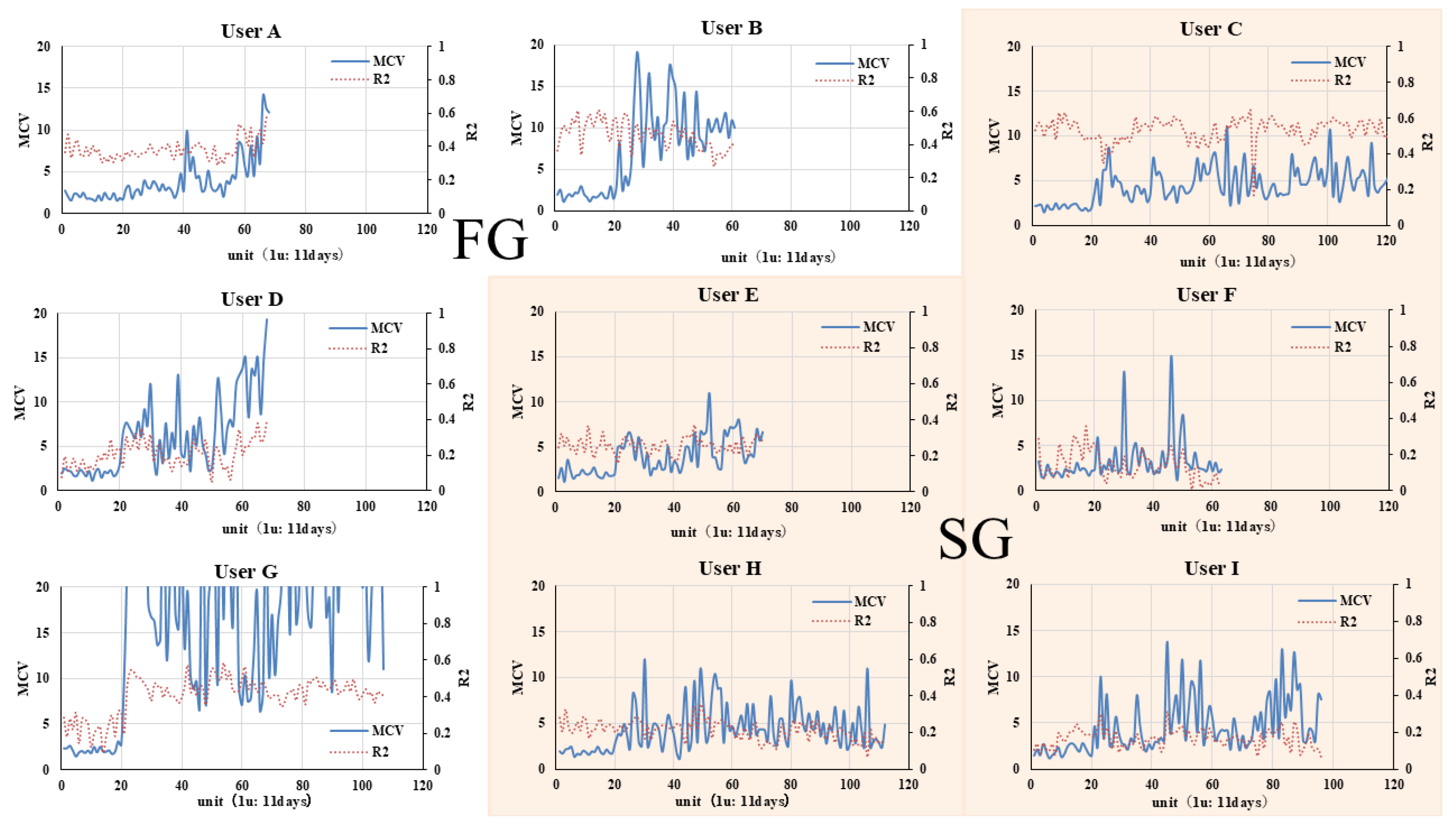
Figure 6.
FRR and FAR between a particular user and the others in SG
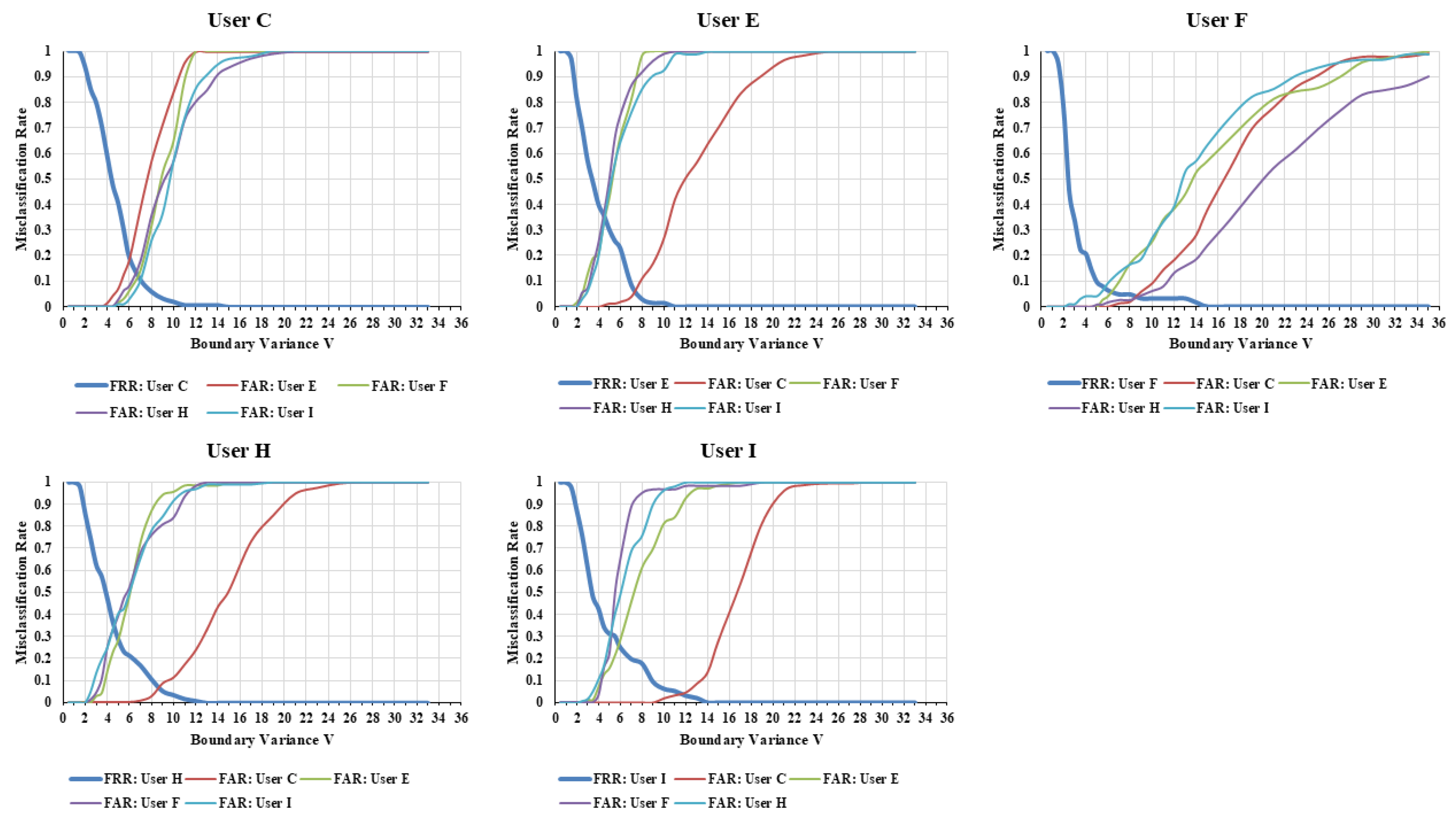
Figure 7.
Misclassification Rate in SG for Each User’s Benchmark Data and Analytical Data by Time
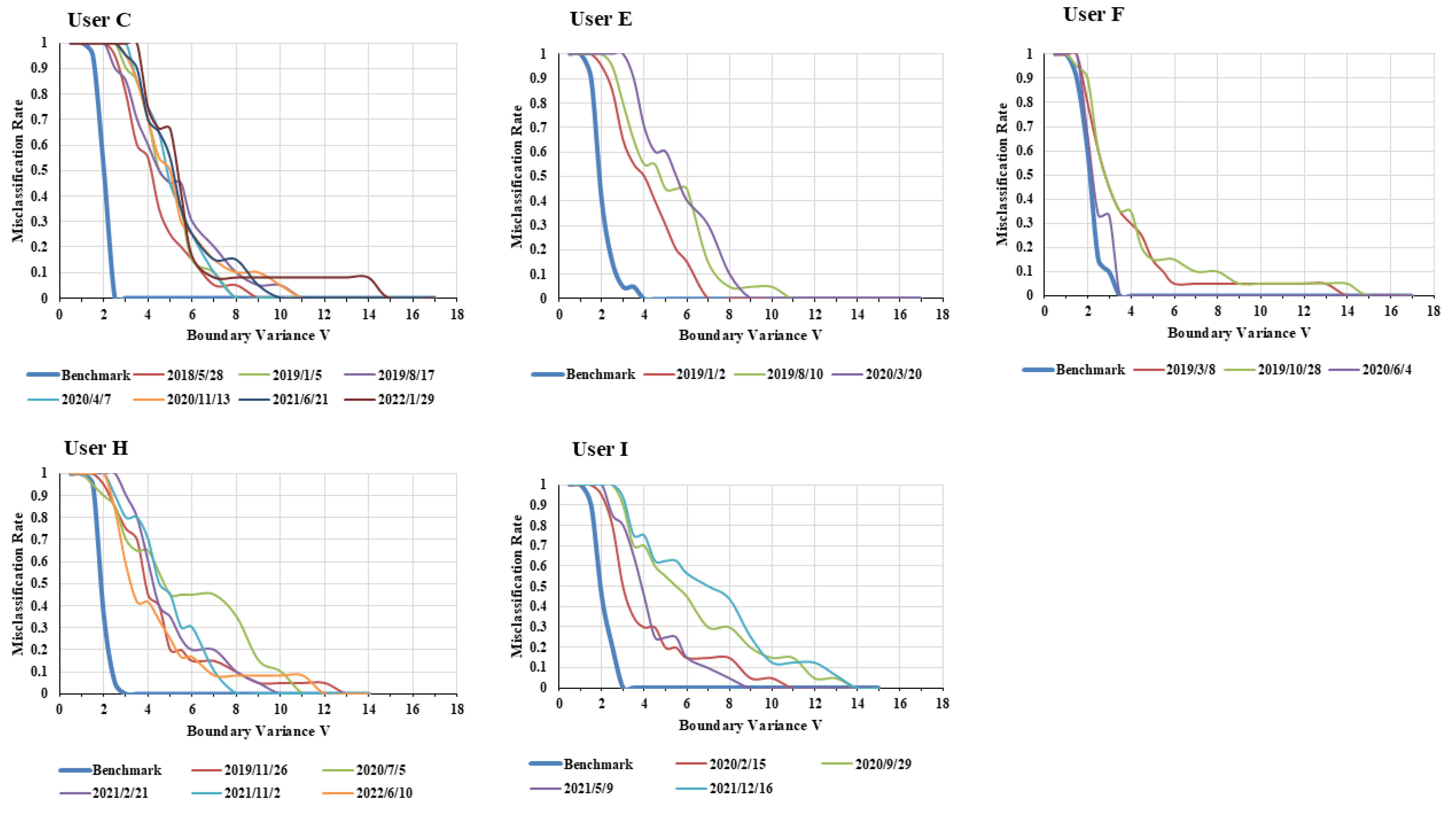
Figure 8.
Misclassification Rate in FG for Each User’s Benchmark Data and Analytical Data by Time
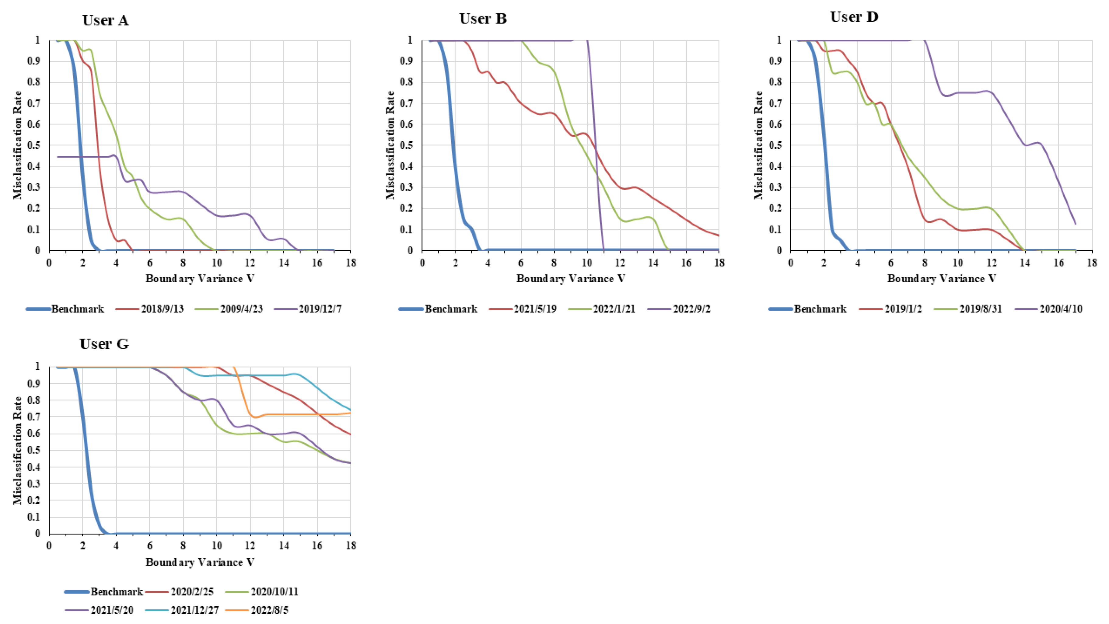

Table 1.
The basic attributes of the subjects and the data used for analysis.
| User | Sex1 | Age | Care Level2 | Residential Style3 | Comorbidity4 | Number of Dataset | Dataset acquisition period | Dataset acquisition days |
|---|---|---|---|---|---|---|---|---|
| A | f | 70s | NC | LA | NO | 75,840 | 2018/01/09-2020/03/14 | 777 |
| B | f | 70s | NC | LA | NO | 66,520 | 2020/09/20-2022/09/14 | 673 |
| C | m | 80s | NC | WF | Hypertension, Angina | 164,660 | 2017/09/27-2022/07/03 | 1,680 |
| D | f | 80s | 4 | LA | Hypertension, Depression, Dementia | 74,608 | 2018/05/25-2020/07/14 | 755 |
| E | m | 60s | NC | WF | NO | 75,436 | 2018/05/25-2020/07/18 | 781 |
| F | f | 80s | 4 | LA | Dementia | 67,636 | 2018/07/31-2020/07/13 | 700 |
| G | f | 80s | 2* | LA | Hypertension, MCI, Rheumatism | 115,968 | 2019/04/14-2022/10/29 | 1,186 |
| H | m | 80s | 2* | LA | Hypertension, Stroke, Osteoarthritis | 123,092 | 2019/04/14-2022/10/29 | 1,242 |
| I | f | 90s | 4 | LA | NO | 103,428 | 2019/06/25-2022/06/14 | 1,060 |
1. Sex: m (Male); f (Female). 2. Care Level: NC (no care needed); 1–7 (Support level 1-2, Care Level 1-5, * is Support level). A higher number indicates a
greater need for care and a reduced ability to perform daily activities independently. 3. Residential Style: LA (Living Alone); WF (living With Family). 4. MCI (Mild Cognitive Impairment)
Disclaimer/Publisher’s Note: The statements, opinions and data contained in all publications are solely those of the individual author(s) and contributor(s) and not of MDPI and/or the editor(s). MDPI and/or the editor(s) disclaim responsibility for any injury to people or property resulting from any ideas, methods, instructions or products referred to in the content. |
© 2025 by the authors. Licensee MDPI, Basel, Switzerland. This article is an open access article distributed under the terms and conditions of the Creative Commons Attribution (CC BY) license (http://creativecommons.org/licenses/by/4.0/).
Copyright: This open access article is published under a Creative Commons CC BY 4.0 license, which permit the free download, distribution, and reuse, provided that the author and preprint are cited in any reuse.


