Submitted:
08 December 2025
Posted:
10 December 2025
You are already at the latest version
Abstract
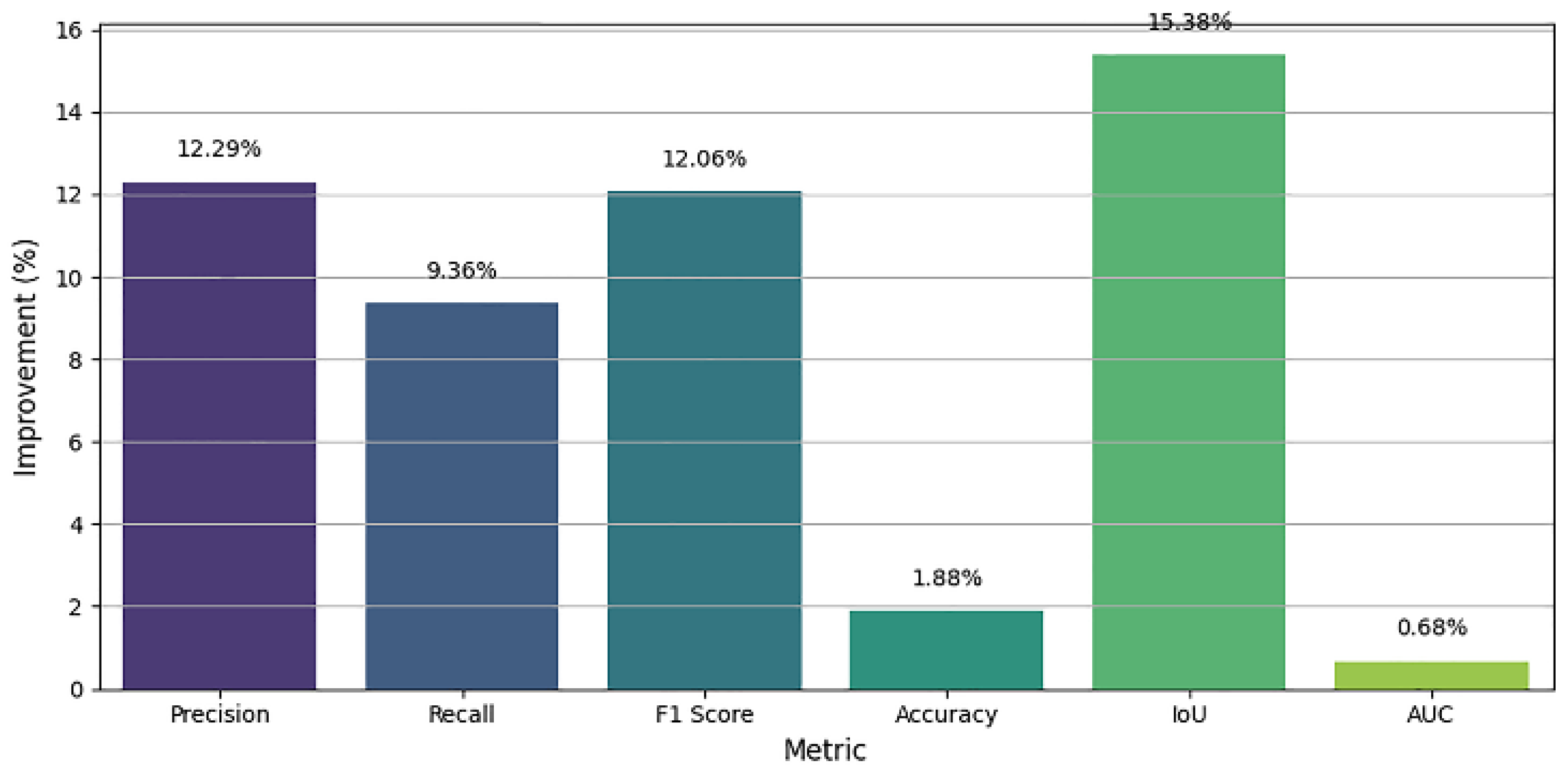
Accurate segmentation of thyroid nodules on ultrasound images remains a challenging task in computer-aided diagnosis (CAD) mainly because of low contrast, speckle noise, and large inter-patient variability of nodule appearance. Here a new deep learning-based segmentation method has been developed on the SwinUNet architecture supported by spatial attention mechanisms to enhance feature discrimination and localization accuracy. The model takes advantage of the hierarchical feature extraction ability of the Swin Transformer to learn both global context and local fine-grained details, whereas attention modules during the decoder process selectively highlight informative areas and suppresses irrelevant background features. We checked out the system's design using the TN3K thyroid ultrasound info that's out there. It got better as it trained, peaking around the 800th run with some good numbers: a Dice Similarity Coefficient (F1 Score) of 85.51%, Precision of 87.05%, Recall of 89.13%, IoU of 78.00%, Accuracy of 97.02%, and an AUC of 99.02%. These numbers are way better than when we started (like a 15.38% jump in IoU and a 12.05% rise in F1 Score), which proves the system can learn tricky shapes and edges well. The longer it trains, the better it gets at spotting even hard-to-see thyroid lumps. This SwinUnet_withAttention thing seems to work great and could be used in clinics to help doctors figure out thyroid problems.
Keywords:
1. Introduction
1.1. Background and Significance
1.2. Related Work and Clinical Background
2. Materials and Methods
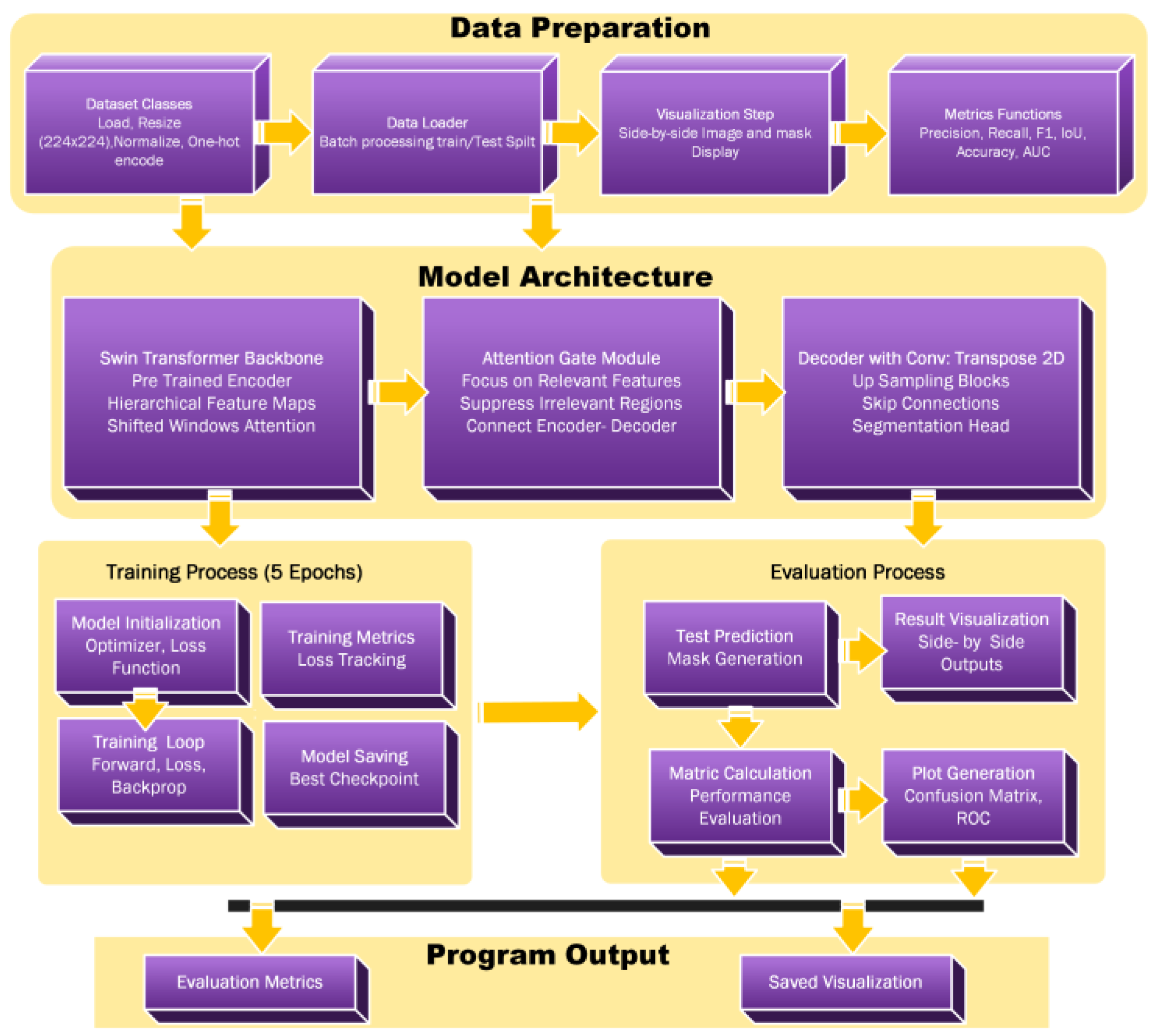
2.1. Flowchart
2.2. Algorithm SwinUnet_ with Attention Mechanism
- - Medical image I ∈ ℝ^(H×W×3)
- - Ground truth mask M ∈ ℝ^(H×W×1)
- - Segmentation Prediction P ∈ ℝ^(H×W×C)
- - Trained model parameters
- Initialize SwinUnet model with Attention Gates
- Load pre-trained Swin Transformer weights
- for each epoch e = 1 to max_epochs do
- for each batch (I, M) ∈ training_data do
- // Forward Pass
- features ← SwinEncoder(I)
- attended_features ← AttentionGates(features)
- P ← Decoder(attended_features)
- // Loss Computation
- loss ← CombinedLoss(P, M)
- // Backward Pass
- optimizer.zero_grad()
- loss.backward()
- optimizer.step()
- end for
- // Validation Phase
- val_metrics ← Evaluate (model, validation_data)
- if val_metrics.improved then
- save_checkpoint(model)
- end if
- end for
- return trained SwinUnet_withAttention model
2.3. Hierarchical Feature Extraction Process
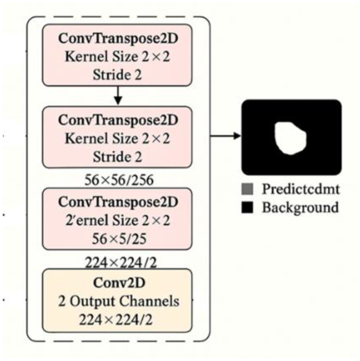
2.3.1. Decoder Architecture for Medical Image Segmentation
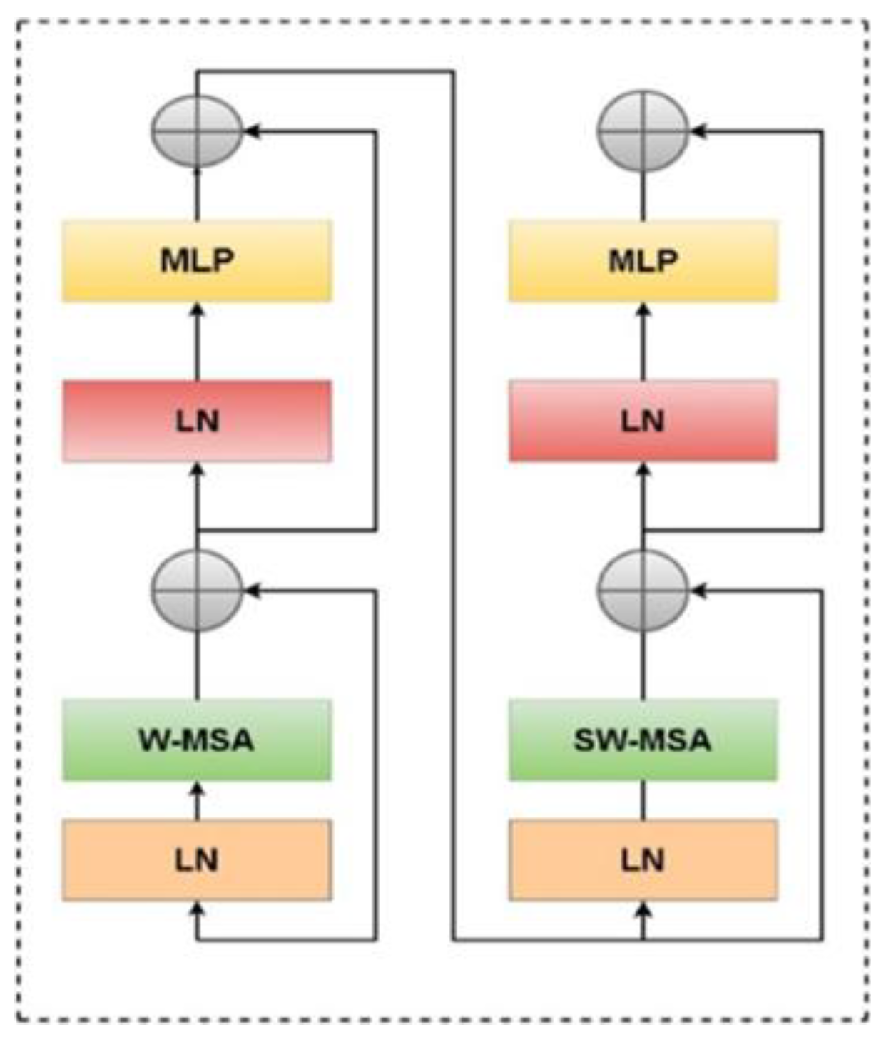
2.3.2. Swin Transformer Block Architecture
2.3.3. Swin Transformer Encoder and Attention Mechanism
2.3.4. Decoder Architecture and Attention Integration
2.4. Experimental Setup and Evaluation Metrics
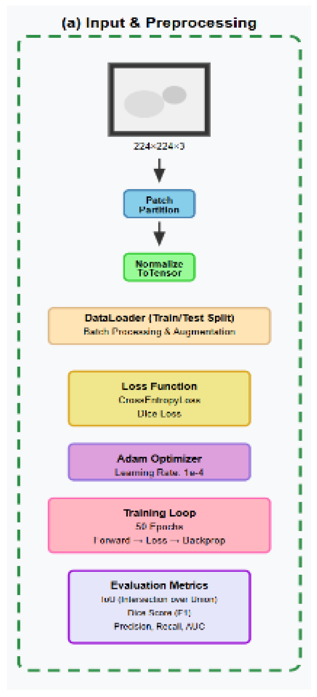
2.4.1. Dataset, Preparation and Preprocessing
2.4.2. Preprocessing, Standardization, and Label Encoding:
2.4.3. Data Augmentation Strategy
- Intersection over Union (IoU)
- Dice Similarity Coefficient:
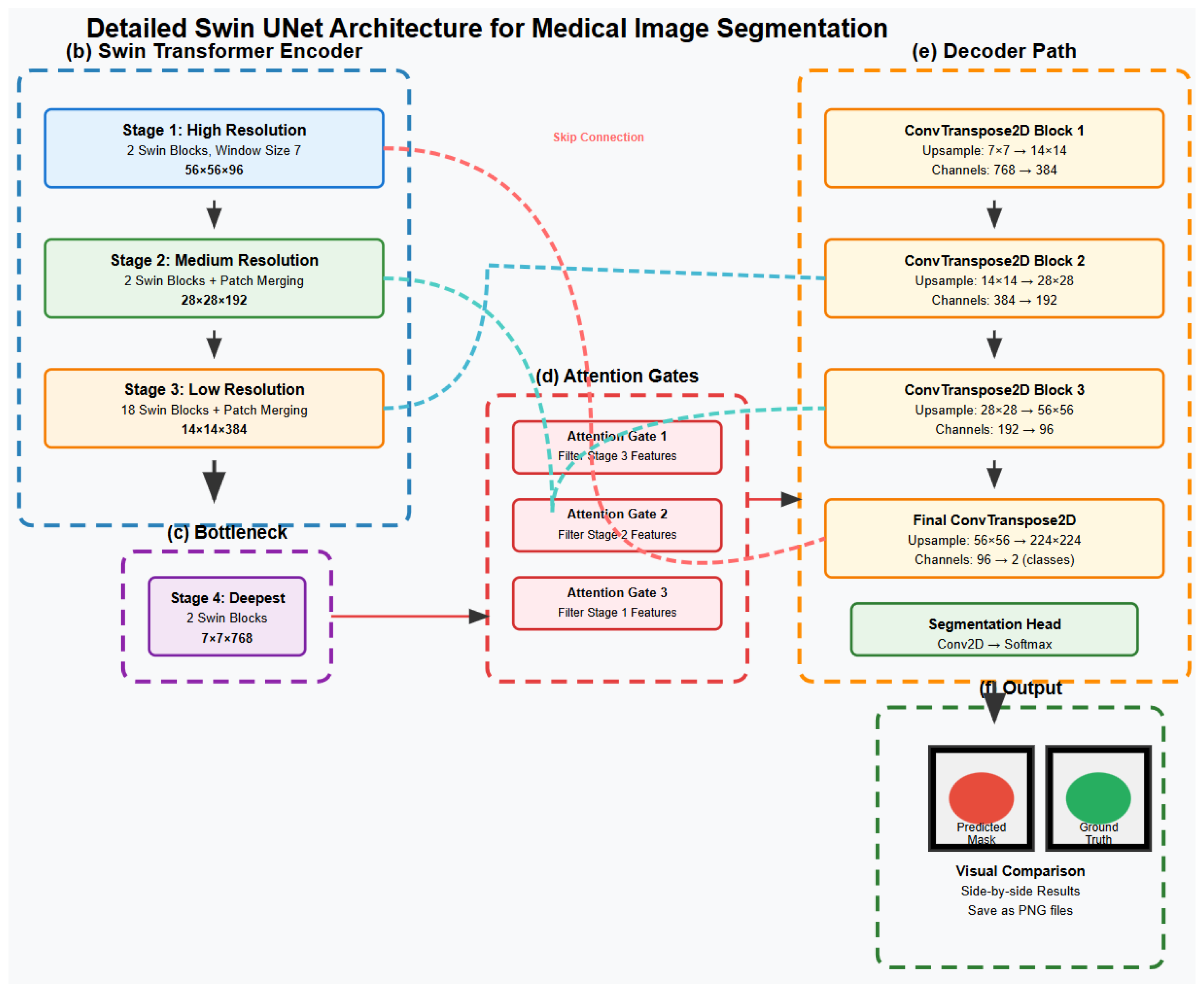
2.5. Complete Swin UNet Architecture for Medical Image Segmentation
3. Results and Discussion
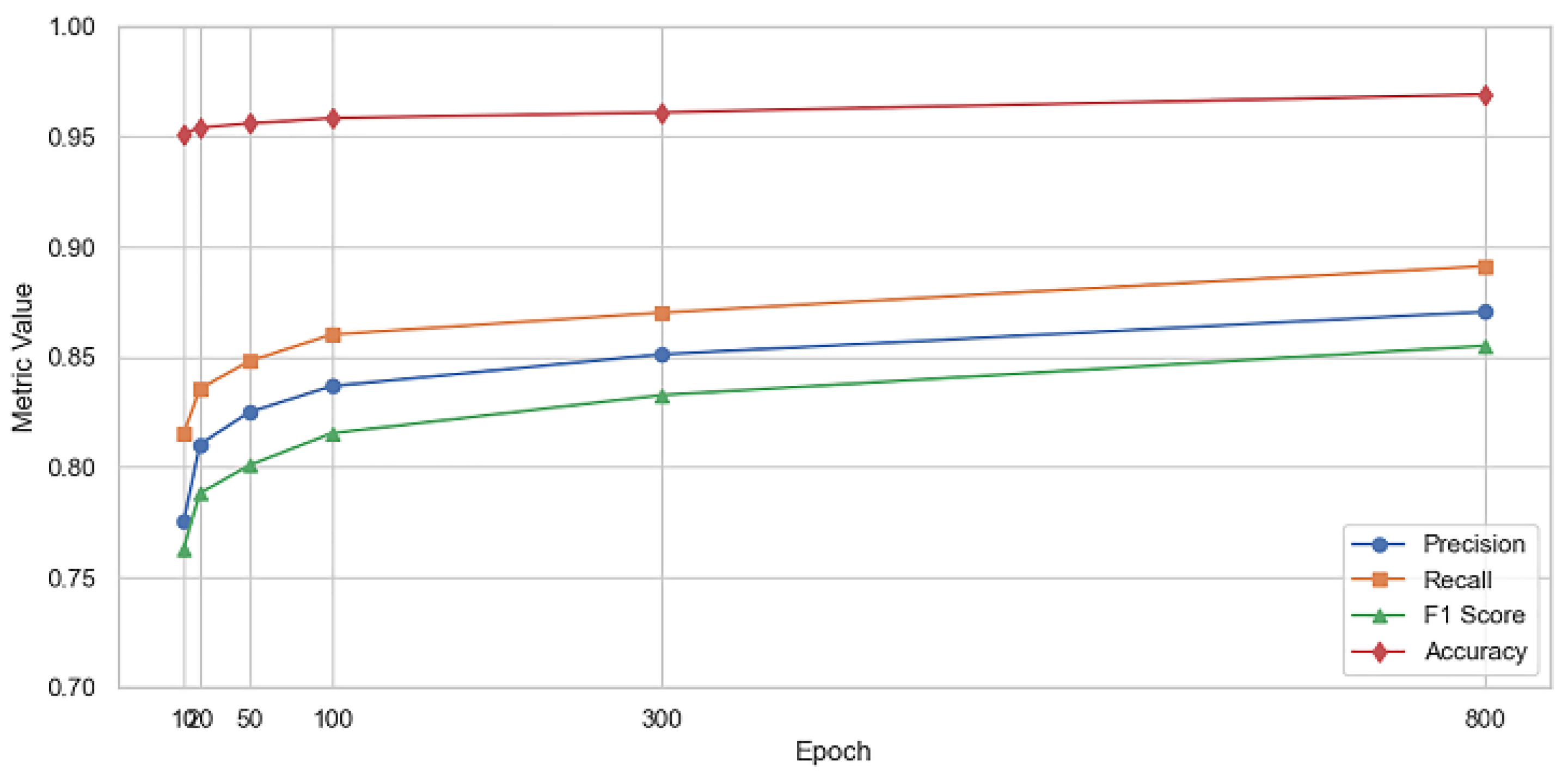
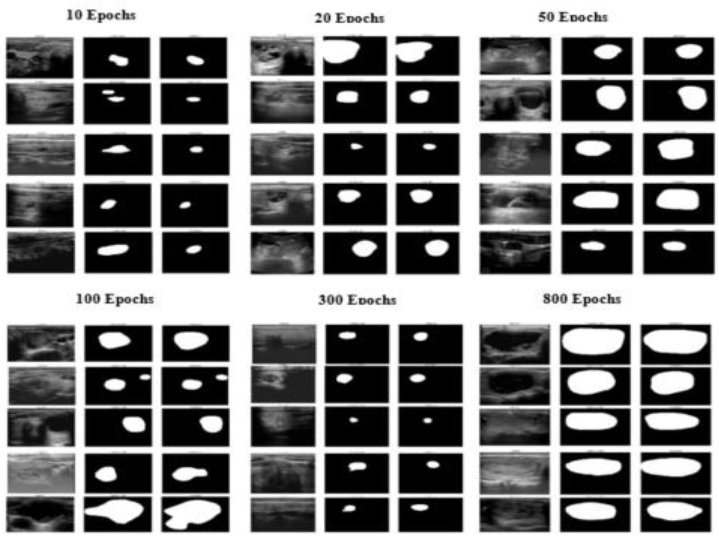
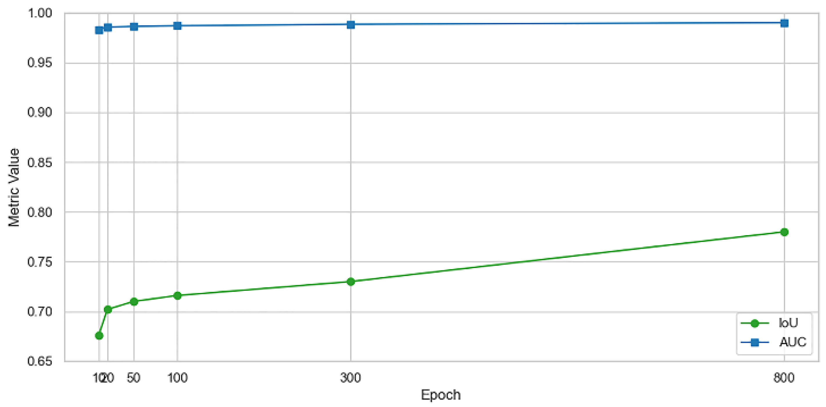
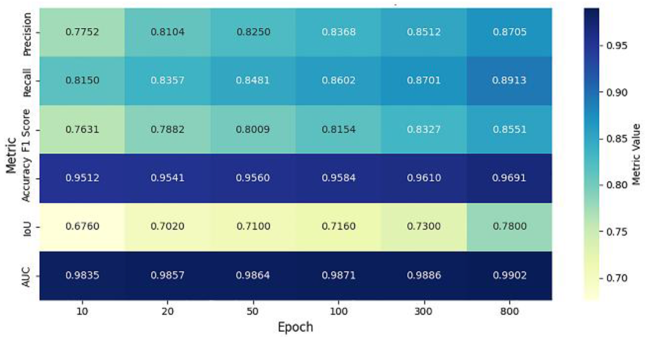
3.1. Performance Evaluation

| Epoch | Precision | Recall | F1 Score | Accuracy | IoU | AUC |
| 10 | 0.7752 | 0.8150 | 0.7631 | 0.9512 | 0.6760 | 0.9835 |
| 20 | 0.8104 | 0.8357 | 0.7882 | 0.9541 | 0.7020 | 0.9857 |
| 50 | 0.8250 | 0.8481 | 0.8009 | 0.9560 | 0.7100 | 0.9864 |
| 100 | 0.8368 | 0.8602 | 0.8154 | 0.9584 | 0.7160 | 0.9871 |
| 300 | 0.8512 | 0.8701 | 0.8327 | 0.9610 | 0.7300 | 0.9886 |
| 800 | 0.8705 | 0.8913 | 0.8551 | 0.9691 | 0.7800 | 0.9902 |


| Epoch | Precision | Recall | F1 Score | Accuracy | IoU | AUC | |
| 10 | - | - | - | - | - | - | |
| 20 | 0.0352 | 0.0207 | 0.0251 | 0.0029 | 0.026 | 0.0022 | |
| 50 | 0.0146 | 0.0124 | 0.0127 | 0.0019 | 0.008 | 0.0007 | |
| 100 | 0.0118 | 0.0121 | 0.0145 | 0.0024 | 0.006 | 0.0007 | |
| 300 | 0.0144 | 0.0099 | 0.0173 | 0.0026 | 0.014 | 0.0015 | |
| 800 | 0.0193 | 0.0212 | 0.0224 | 0.0081 | 0.05 | 0.0016 |
| Metric | Best Value | Epoch |
| Precision | 0.8705 | 800 |
| Recall | 0.8913 | 800 |
| F1 Score | 0.8551 | 800 |
| Accuracy | 0.9691 | 800 |
| IoU | 0.780 | 800 |
| AUC | 0.9902 | 800 |
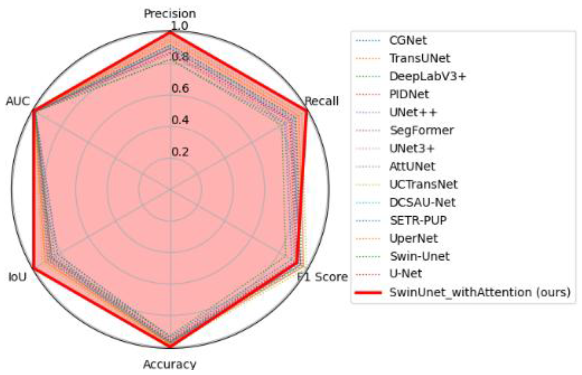
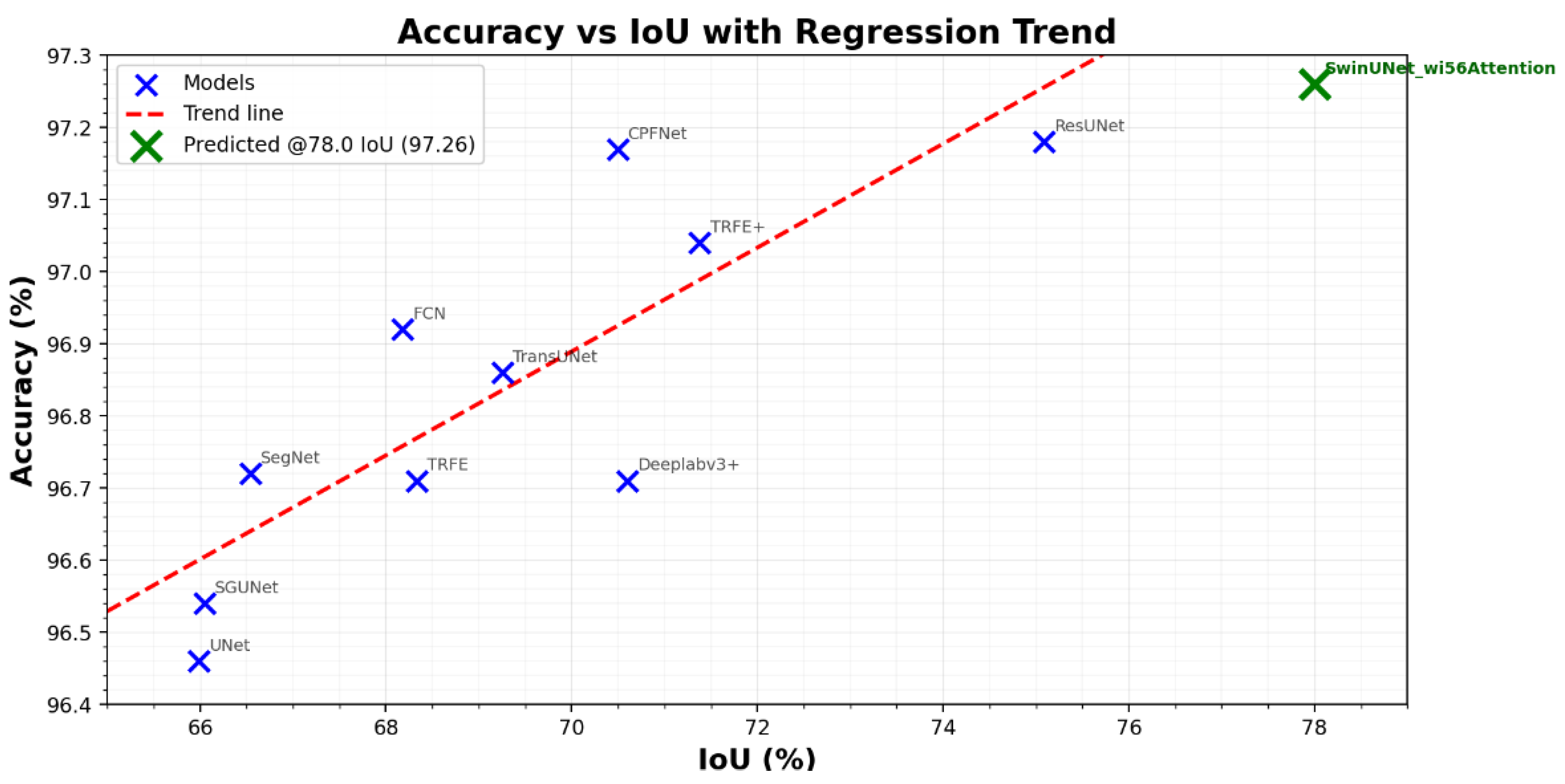
| Model | Dataset | Accuracy (%) | IoU (%) | Dice (%) |
| TransUNet [47] | TN3K train | 96.86 ± 0.05 | 69.26 ± 0.55 | 81.84 ± 1.09 |
| TRFE+ [48] | TN3K train | 97.04 ± 0.10 | 71.38 ± 0.43 | 83.30 ± 0.26 |
| SGUNet [49] | TN3K train | 96.54 ± 0.09 | 66.05 ± 0.43 | 79.55 ± 0.86 |
| UNet [50] | TN3K train | 96.46 ± 0.11 | 65.99 ± 0.66 | 79.51 ± 1.31 |
| ResUNet [51] | TN3K train | 97.18 ± 0.03 | 75.09 ± 0.22 | 83.77 ± 0.20 |
| SegNet [52] | TN3K train | 96.72 ± 0.12 | 66.54 ± 0.85 | 79.91 ± 1.69 |
| FCN [53] | TN3K train | 96.92 ± 0.04 | 68.18 ± 0.25 | 81.08 ± 0.50 |
| CPFNet [54] | TN3K train | 97.17 ± 0.06 | 70.50 ± 0.39 | 82.70 ± 0.78 |
| Deeplabv3+ [55] | TN3K train | 97.19 ± 0.05 | 70.60 ± 0.49 | 82.77 ± 0.98 |
| TRFE [56] | TN3K train | 96.71 ± 0.07 | 68.33 ± 0.68 | 81.19 ± 1.35 |
| SwinUNet_wi56Attention (our) | TN3K train | 96.91 ± 0.00 | 78.00 ± 0.00 | 87.60 ± 0.00 |
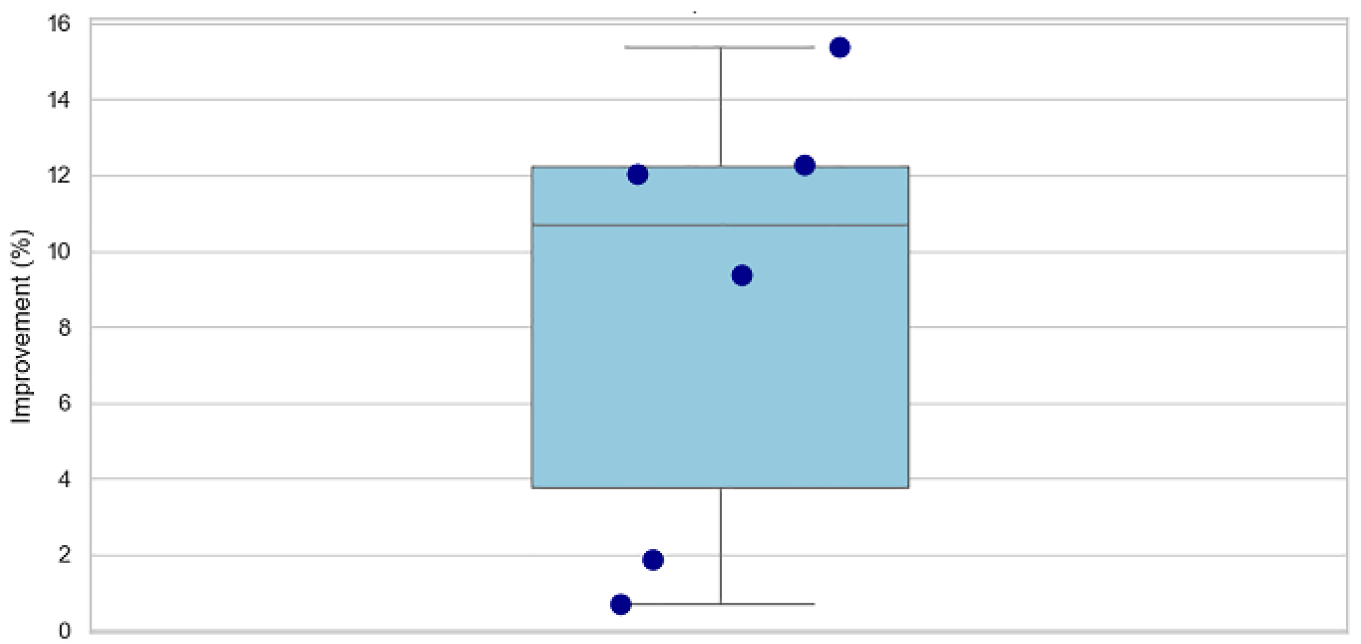
- Performance Gains
3.2. Discussion
4. Conclusion
- Future Recommendations:
Author Contributions
Funding
Data Availability Statement
Conflicts of Interest
References
- Zhuo, X.; Zhang, Y.; Wang, L. Neural Networks. Neural Netw. 2024, 181, 106754. [Google Scholar]
- Yang, C.; Li, H.; Zhang, Q. Swin U-Net for thyroid nodule segmentation. Front. Oncol. 2025, 15, 1456563. [Google Scholar]
- Munsterman, R.; van der Velden, T.; Jansen, K. 3D ultrasound segmentation of thyroid. WFUMB Ultrasound Open 2024, 2, 100055. [Google Scholar] [CrossRef]
- Li, X.; Chen, Y.; Liu, Z. DMSA-UNet for medical image segmentation. Knowl.-Based Syst. 2024, 299, 112050. [Google Scholar] [CrossRef]
- Li, X.; et al. Thyroid ultrasound image database. Ultrasound Med. Biol. 2023. [Google Scholar]
- Chaphekar, M.; Chandrakar, O. An improved deep learning models with hybrid architectures thyroid disease classification diagnosis. J. Neonatal Surg. 2025, 14, 1151–1162. Available online: https://www.jneonatalsurg.com/index.php/jns/article/view/1925. [CrossRef]
- Wang, J.; Zhao, L.; Chen, M. Deep learning for thyroid FNA diagnosis. Lancet Digit. Health 2024, 6. [Google Scholar]
- Yadav, N.; Kumar, S.; Singh, P. ML review on thyroid tumor via ultrasound. J. Ultrasound 2024, 27, 209–224. [Google Scholar] [CrossRef]
- Cantisani, V.; et al. Multiparametric ultrasound in thyroid nodules. Ultrasound 2025, 46, 14–35. [Google Scholar]
- Gulame, M.B.; Dixit, V.V. Hybrid DL for thyroid grading. Int. J. Numer. Meth. Biomed. Engng. 2024, 40. [Google Scholar]
- Lu, X.; Xu, W.; Zhao, H. MAGCN for synthetic lethality prediction. IEEE/ACM Trans. Comput. Biol. Bioinform. 2023, 20, 2591–2602. [Google Scholar] [CrossRef]
- Che, X.; Wang, F.; Deng, Y. Case-based reasoning for thyroid diagnosis. Knowl.-Based Syst. 2022, 251, 109234. [Google Scholar]
- Gong, H.; Zhou, M.; Wu, J. Attention-guided thyroid segmentation. Comput. Biol. Med. 2023, 155, 106641. [Google Scholar] [CrossRef] [PubMed]
- Yetginler, B.; Atacak, I. Improved V-Net for thyroid segmentation. Appl. Sci. 2025, 15, 3124. [Google Scholar] [CrossRef]
- Dong, P.; Wei, Y.; Guo, L. Dual-path attention UNet++. BMC Med. Imaging 2024, 24, 341. [Google Scholar]
- Chen, Y.; Wang, X.; Li, Z. Thyroid segmentation with boundary improvement. Appl. Intell. 2023, 53, 18312–18325. [Google Scholar]
- Das, D.; Roy, A.; Mukherjee, S. DL for thyroid nodule examination. Artif. Intell. Rev. 2024, 57, 78. [Google Scholar] [CrossRef]
- Ma, X.; Sun, Y.; Feng, Z. AMSeg for thyroid segmentation. IEEE Access 2023, 11, 98765–98776. [Google Scholar]
- Beyyala, A.; Polat, K.; Kaya, M. Swin Transformer for thyroid segmentation. Ingénierie des Systèmes d’Information 2024, 29, 123–130. [Google Scholar]
- Yang, W.-T.; Lin, C.-H.; Chen, S.-K. Deep learning in thyroid imaging. Quant. Imaging Med. Surg. 2024, 14, 2023–2037. [Google Scholar] [CrossRef]
- Sureshkumar, V.; Priya, R.; Geetha, N. Transfer learning for thyroid nodule classification. Curr. Comput.-Aided Drug Des. 2024. [Google Scholar]
- Sabouri, M.; Gholami, P.; Khosravi, A. Thyroidiomics: Scintigraphy pipeline. arXiv 2024, arXiv:2407.10336. [Google Scholar]
- Mau, M.; Schmidt, A.; Weber, T. Thyroid Scintigram segmentation. Proc. Bildverarbeitung für die Medizin, 2025; pp. 123–128. [Google Scholar]
- Prochazka, A.; Zeman, J. U-Net with ResNet encoder. AIMS Med. Sci. 2025, 12, 45–58. [Google Scholar]
- Chi, J.; Li, Z.; Sun, Z.; Yu, X.; Wang, H. Hybrid transformer UNet for thyroid segmentation from ultrasound scans. Comput. Biol. Med. 2023, 153, 106453. [Google Scholar] [CrossRef] [PubMed]
- Peng, B.; Huang, L.; Xia, Y. DC-Contrast U-Net. BMC Med. Imaging 2024, 24, 275. [Google Scholar]
- Haribabu, K.; Siva, S.; Venkateswarlu, T. MLRT-UNet. Comput. Model. Eng. Sci. 2025, 143, 413–448.
- Agustin, S.; Wijaya, D.; Santoso, R. Residual U-Net for detection and classification. Automatika 2024, 65, 726–737. [Google Scholar] [CrossRef]
- Zeng, Y.; Bao, X.; Liu, F. CT segmentation via U-Net. Proc. SPIE 2023, 12705, 127050L. [Google Scholar]
- Chen, Y.; Wang, X.; Li, Z. Super-pixel U-Net for thyroid segmentation. Ultrasound Med. Biol. 2023, 49, 1923–1932. [Google Scholar]
- Chi, J.; Zhang, H.; Yu, L. Hybrid transformer U-Net. Comput. Biol. Med. 2023, 153, 106516. [Google Scholar]
- Ajilisa, O.; Mathew, T.; Soman, K.P. CNNs for thyroid segmentation. J. Intell. Fuzzy Syst. 2022, 43, 1235–1246. [Google Scholar]
- Arepalli, L.; Reddy, R.; Kumar, V. Soft computing for thyroid nodules. Soft Comput. 2025, 29, 1789–1805. [Google Scholar]
- Xu, Y.; Li, M.; Zhang, J. Review on medical image segmentation. Bioengineering 2024, 11, 363. [Google Scholar]
- Al-Mukhtar, F.H.; Ali, A.A.; Al-Dahan, Z.T. Joint segmentation and classification. ZJPAS 2024, 36, 112–125. [Google Scholar]
- Yang, D.; Liu, Y.; Wang, H. Multi-task thyroid tumor segmentation. Biomed. Signal Process. Control 2023, 79, 104072. [Google Scholar] [CrossRef]
- Xu, P. Research on thyroid nodule segmentation using an improved U-Net network. Rev. int. métodos numér. cálc. diseño ing. 2024, 40, 1–7. [Google Scholar] [CrossRef]
- Ozcan, A.; Yildirim, S.; Demir, M. Enhanced-TransUNet. Biomed. Signal Process. Control 2024, 95, 106289. [Google Scholar]
- Shao, J.; Mei, L.; Fang, C. FCG-Net for thyroid segmentation. Biomed. Signal Process. Control 2023, 86, 105312. [Google Scholar]
- Hu, R.; Cai, Y.; Dong, W. Improved U-Net. IAENG Int. J. Comput. Sci. 2025, 52, 612–623. [Google Scholar]
- Pan, H.; Liu, Y.; Wei, Z. SGUNET. Proc. IEEE Int. Symp. Biomed. Imaging (ISBI), 2021; pp. 630–634. [Google Scholar]
- Xu, P. Improved U-Net for thyroid segmentation. Rev. int. métodos numér. cálc. diseño ing. 2024, 40. [Google Scholar] [CrossRef]
- Zhang, J.; Wang, Y.; Zhao, L. ST-Unet: Swin Transformer U-Net. Comput. Biol. Med. 2023, 153, 106579. [Google Scholar]
- Li, Y.; Zou, Y.; He, X.; Xu, Q.; Liu, M.; Chen, Z.; Yan, L.; Zhang, J. HFA-UNet: Hybrid and full-attention UNet for thyroid nodule segmentation. Knowledge-Based Systems 2025, 328, 114245. [Google Scholar] [CrossRef]
- Ajilisa, O.A.; Jagathy Raj, V.P.; Sabu, M.K. Segmentation of thyroid nodules from ultrasound images using convolutional neural network architectures. J. Intell. Fuzzy Syst. 2022, 43, 687–705. [Google Scholar] [CrossRef]
- Yang, C.; Li, H.; Zhang, Q. Swin U-Net model. Front. Oncol. 2025, 15, 1456563. [Google Scholar] [CrossRef]
- Chen, J.; Lu, Y.; Yu, Q.; et al. TransUNet: Transformers Make Strong Encoders for Medical Image Segmentation. 2021. Available online: https://arxiv.org/abs/2102.04306.
- Gong, H.; Chen, J.; Chen, G.; et al. Thyroid Region Prior Guided Attention for Ultrasound Segmentation of Thyroid Nodules. 2023. Available online: https://arxiv.org/abs/2307.XXXX.
- Pan, H.; Zhou, Q.; Latecki, L.J. SGUNet: Semantic Guided U-Net for Thyroid Nodule Segmentation. In Proceedings of the 2021 IEEE International Conference on Image Processing (ICIP), 2021; pp. xxxx–xxxx. [Google Scholar]
- Ronneberger, O.; Fischer, P.; Brox, T. U-Net: Convolutional Networks for Biomedical Image Segmentation. In Proceedings of the International Conference on Medical Image Computing and Computer-Assisted Intervention (MICCAI), 2015; Springer: Cham, Switzerland; pp. 234–241. [Google Scholar]
- Prochazka, A.; Zeman, J. Thyroid Nodule Segmentation in Ultrasound Images Using U-Net with ResNet Encoder: Achieving State-of-the-Art Performance on All Public Datasets. AIMS Med. Sci. 2025, 12, 124–144. [Google Scholar] [CrossRef]
- Badrinarayanan, V.; Kendall, A.; Cipolla, R. SegNet: A Deep Convolutional Encoder–Decoder Architecture for Image Segmentation. IEEE Trans. Pattern Anal. Mach. Intell. 2017, 39, 2481–2495. [Google Scholar] [CrossRef] [PubMed]
- Long, J.; Shelhamer, E.; Darrell, T. Fully Convolutional Networks for Semantic Segmentation. In Proceedings of the IEEE Conference on Computer Vision and Pattern Recognition (CVPR), 2015; pp. 3431–3440. [Google Scholar]
- Feng, S.; Zhao, H.; Shi, F.; et al. CPFNet: Context Pyramid Fusion Network for Medical Image Segmentation. 2020. Available online: https://arxiv.org/abs/2009.07129.
- Chen, L.-C.; Zhu, Y.; Papandreou, G.; et al. Encoder–Decoder with Atrous Separable Convolution for Semantic Image Segmentation. In Proceedings of the European Conference on Computer Vision (ECCV), 2018; pp. 801–818. [Google Scholar]
- Gong, H.; Chen, G.; Wang, R.; et al. Multi-Task Learning for Thyroid Nodule Segmentation with Thyroid Region Prior. In Proceedings of the 2021 IEEE 18th International Symposium on Biomedical Imaging (ISBI), Nice, France, 13–16 April 2021; pp. 257–261. [Google Scholar] [CrossRef]


| Stage | Output Size | Feature Depth | Feature Type |
| 1 | 56×56×C | Low | Shallow (Local textures) |
| 2 | 28×28×512 | Medium | Mid-level patterns |
| 3 | 14×14×512 | High | Deep semantic features |
| 4 | 7×7×1024 | Very High | Global contextual features |
| Metric | Epoch 10 | Epoch 800 | % Increase |
| Precision | 0.7752 | 0.8705 | +12.3% |
| Recall | 0.815 | 0.8913 | +9.37% |
| F1 Score | 0.7631 | 0.8551 | +12.05% |
| Accuracy | 0.9512 | 0.9691 | +1.88% |
| IoU | 0.676 | 0.780 | +15.38% |
| AUC | 0.9835 | 0.9902 | +0.68% |
Disclaimer/Publisher’s Note: The statements, opinions and data contained in all publications are solely those of the individual author(s) and contributor(s) and not of MDPI and/or the editor(s). MDPI and/or the editor(s) disclaim responsibility for any injury to people or property resulting from any ideas, methods, instructions or products referred to in the content. |
© 2025 by the authors. Licensee MDPI, Basel, Switzerland. This article is an open access article distributed under the terms and conditions of the Creative Commons Attribution (CC BY) license (http://creativecommons.org/licenses/by/4.0/).


