Submitted:
08 December 2025
Posted:
09 December 2025
You are already at the latest version
Abstract
Urban renewal research has long relied on expert-led assessments and fragmented indicators, yet lacks scalable, perception-aware frameworks that can translate street-level conditions into interpretable renewal strategies. To bridge these gaps, this study proposes a vision–language model (VLM) based method to identify the potentially renewable areas across the Hongshan Central District of Urumqi, China. Specifically, we collected 4,215 panoramas and used multiple VLMs to measure six perceptual scores (i.e., safety, liveliness, beauty, wealthiness, depressiveness, and boringness) together with textual descriptions. The best-performing model, selected by correlation with a 500-respondent perception survey, was used as the final analysis to identify the renewal area. Then, we conducted spatial statistics and text mining (eight semantic themes) to reveal the spatial patterns and semantic topics for proposing renewal strategies. The results show that: 1) VLMs have a high consistency with humans in evaluating the spatial perception of six dimensions; 2) four renewal priority tiers were identified, with high-score areas concentrated on Tianshan District Government Residential Quarter, Mashi Community, Heping South Road, etc.; and 3) Semantically, low-score areas such as Hongshan Road, Binhe Middle Road, Wuxing South Road, Huhuo Line, etc. emphasize infrastructure, safety, street level and order. We conclude that VLMs add value not only via scalable assessment but also through explanatory language evidence that directly supports tiered renewal and public communication. This work provides a data-driven and interpretable evaluation framework for urban renewal decision-making, facilitating precision-oriented and intelligent regional urban regeneration.
Keywords:
urban perception
; street-view imagery
; vision–language model
; spatial autocorrelation
; text semantics
; urban renewal
1. Introduction
Over the past decade, urban planning in China has shifted from high-speed expansion to the stock-optimization phase, marking a strategic shift from scale growth and factor inputs to renewal practices centered on quality enhancement, structural repair, and fine-grained governance [1,2,3]. A fundamental question in this transition is how to measure “urban spatial quality” in a scientific, comparable, and operational manner [4]. Such measurement considers not only objective physical indicators but also people’s subjective perception and experience. For instance, as early as the 1960s, Kevin Lynch [5] emphasized in The Image of the City that the material environment shapes residents’ mental images, with paths, edges, districts, nodes, and landmarks jointly forming a legible urban image. Jane Jacobs [6] subsequently proposed the “eyes on the street,” arguing that streets animated by pedestrian flow and natural surveillance can substantially improve the sense of safety. Conversely, neighborhood dilapidation undermines safety and belonging, as classically articulated by Wilson and Kelling’s [7] “broken windows” hypothesis. Recent studies have shown that the aesthetic quality of streetscapes not only enhances urban attractiveness but is also positively associated with mental and physical health [8,9,10]. Together, these studies underscore that the visual quality of the built environment is tightly linked to subjective feelings; dimensions such as safety, vitality, and beauty have become key determinants of urban spatial success [11,12]. These converging insights demonstrate that visual perception is not merely an aesthetic consideration but a fundamental determinant of urban livability.
Traditionally, urban perception has been assessed through questionnaires and field audits. However, these methods are costly and time-consuming, making it difficult to describe perceptual differences street by street at the city scale [13,14]. Over the past decade, with the rise of crowdsourcing and computer vision, researchers began to use street-view images (SVIs) and machine learning to quantify perception [15]. For example, Salesses et al. [16] collected public judgments via online pairwise image comparisons to build large-scale datasets of subjective evaluations (e.g., safety, prosperity), revealing spatial inequalities in urban perception. The Place Pulse 2.0 dataset developed at MIT Media Lab, as described by Dubey et al. [17], further distilled urban perception into six dimensions—Safety, Liveliness, Beauty, Wealthiness, and the opposing attributes Depressiveness and Boringness. Building on this, previous approaches usually relied on deep learning or machine learning. Specifically, Zhang et al. [18] achieved high accuracy in inferring perceptual attributes such as safety and beauty by employing Deep Spatial Attention Neural Zero-Shot (DSANZS) models with supervised and weakly supervised learning on the Place Pulse 2.0 dataset. Additionally, Contrastive Language-Image Pre-Training (CLIP)-based zero-shot methods have demonstrated high accuracy in urban perception analysis. For example, CLIP was successfully employed by Liu et al. [19] to build reliable perceived walkability indicators and by Zhao et al. [20] to accurately quantify the visual quality of built environments for aesthetic and landscape evaluation. However, although these approaches substantially reduce labeling costs and provide an end-to-end solution, they still require adaptation to local context and offer limited interpretability.
On the other hand, with the rise of computer vision technology, many models have been developed to segment street-view elements and correlate them with perception using machine learning approaches. Semantic segmentation models such as DeepLab [21] and PSPNet [22] can identify and quantify various urban elements such as buildings, vegetation, vehicles, and pedestrians in street imagery, providing objective measures of streetscape composition. These segmented elements are then linked to perceptual outcomes through statistical modeling or machine learning algorithms. For instance, Kang et al. [23] used semantic segmentation to extract 150 visual elements from street-view images and employed random forest regression to predict safety perception scores, finding that the proportion of sky, trees, and crosswalks positively influenced perceived safety while cars and construction elements had negative effects. Furthermore, explainable artificial intelligence techniques, particularly SHapley Additive exPlanations (SHAP) [24], offer opportunities to open the “black box” of machine learning models by revealing which visual elements contribute most to specific perceptual judgments. For example, researchers have used SHAP values to demonstrate that the presence of greenery and well-maintained facades positively correlates with safety perception. However, these element-based approaches often oversimplify the complex interactions between urban features and may miss subtle contextual factors that influence human perception, thus limiting their ability to capture the holistic nature of urban perception.
In recent years, vision–language models (VLMs) have provided new tools for urban perception research. Large multimodal models such as LLaVA, BLIP-2, and CLIP integrate image understanding with natural-language reasoning and can analyze images in a human-like, instruction-following manner without additional local training, as demonstrated by Moreno-Vera and Poco [25]. In the urban domain, scholars have begun to explore VLMs for street-scene parsing and evaluation. For example, Yu et al. [26] extracted street-scene elements with deep learning and, supported by adversarial modeling, quantified the six perception dimensions, combining the results with space-syntax analysis to reveal links between streetscape quality and element configuration. Moreover, VLMs can simultaneously process visual information and generate actionable recommendations for urban improvement, offering a more comprehensive approach than traditional perception analysis methods. This suggests that, without relying on locally labeled data, pretrained VLMs can be used to assess streetscape perception in any city, thereby lowering data costs and improving generalization.
Against this backdrop, this study seeks to address three key research questions that guide our investigation: (1) How accurately can VLMs predict human perceptual judgments across the six urban perception dimensions compared to traditional survey methods? (2) What are the spatial patterns and salient characteristics that VLMs identify in different urban areas, and how do these align with human observations? (3) To what extent can VLMs generate actionable and contextually appropriate renewal suggestions for urban planning practice? To answer these questions, we integrate multimodal VLMs with SVIs using the Hongshan Central District of Urumqi, China, as our study area. We collected 4,215 street-view panoramas and conducted a perception survey with 500 respondents across the six dimensions to establish a human-rated baseline. We then applied multiple VLMs to measure Safety, Liveliness, Beauty, Wealthiness, Depressiveness, and Boringness, accompanied by textual explanations and renewal suggestions. By systematically comparing model outputs with survey results and mining keywords from model descriptions, we evaluate VLM performance boundaries and explore their potential as decision support tools for intelligent urban planning.
2. Materials and Methods
2.1. Study Area
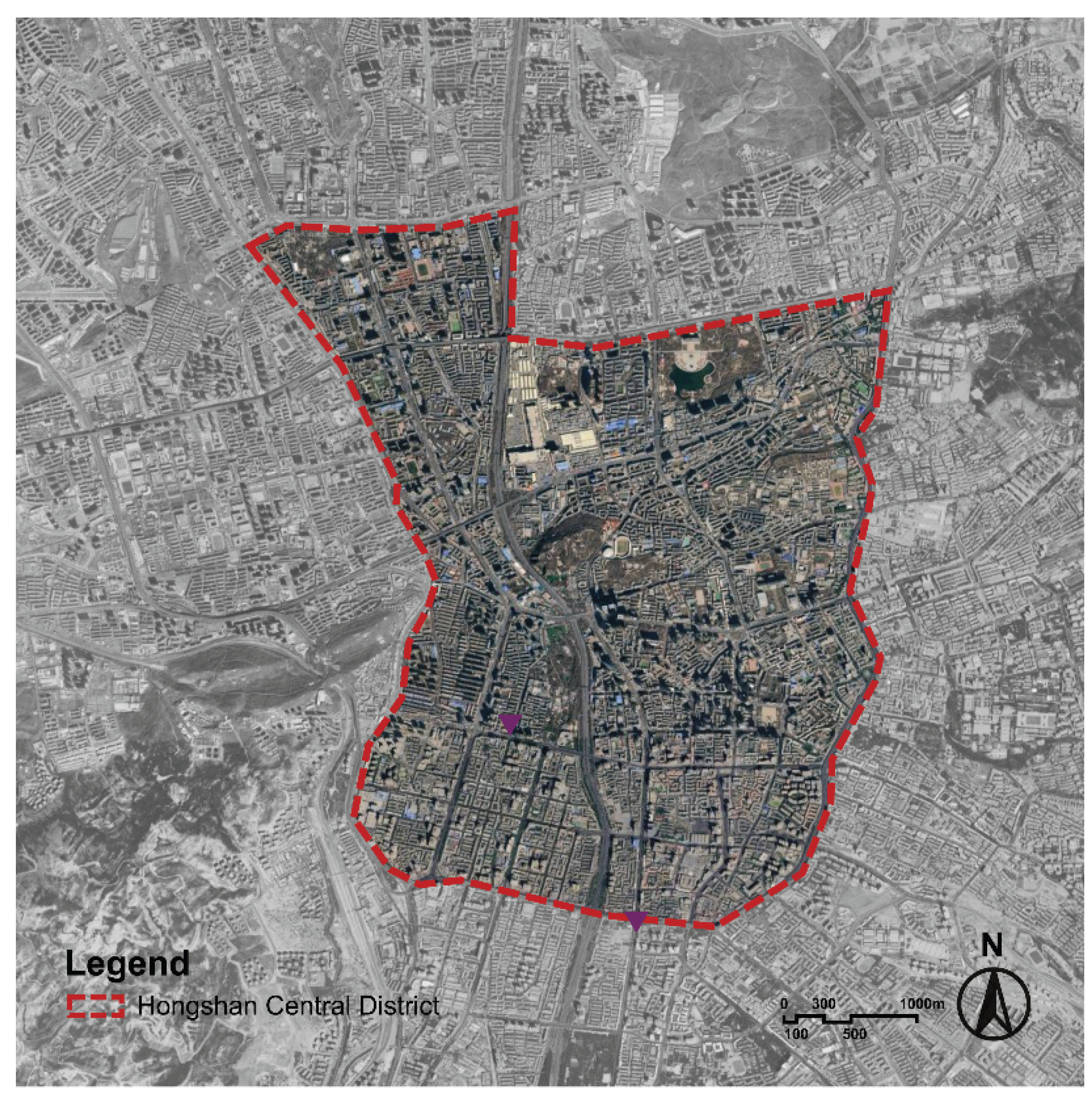
The Hongshan Central District is in the urban core of Urumqi, China, spanning Tianshan, Shayibake, and Shuimogou districts. It is a mixed area of commerce, culture, and housing. Within an area of 20 km², we obtained 4,215 street-view panoramas from Baidu Street View between April and August 2024, covering arterials, secondary streets, alleys, and key nodes (e.g., Hongshan Park, commercial streets, residential compounds, and school environs). The sampling points were systematically distributed at 50-meter intervals along the road network to ensure comprehensive spatial coverage while maintaining computational feasibility. To ensure data quality, we implemented a multi-stage screening process: 1) panoramas with poor visibility (fog, heavy shadows, or construction obstructions) were automatically filtered using image clarity metrics; 2) duplicate or near-duplicate images within 10 meters of each other were removed to avoid spatial redundancy; and 3) manual verification was conducted on a random sample of 500 images to validate the automated screening results, achieving 94% accuracy in quality assessment. These data underpin the subsequent model evaluation and spatial analysis.
Figure 1.
Pipeline of respondent-persona scoring and expert planning with structured outputs.
2.2. VLM Selection and Prompt Design
Our methodological workflow is illustrated in Figure 2, comprising four main components. In Step 1, we instantiate an LLM-simulated respondent persona, whose demographic slots reflect real-world survey distributions (as shown in section 2.3). The persona is coupled with task prompts so that the model reasons from a lay inhabitant’s perspective rather than an expert’s viewpoint. In Step 2, we provide the VLMs with SVI and scoring instructions to constrain the model to judge based on visible cues and subjective spatial perception, assigning integer scores from 1 to 10 for safety, vitality, beauty, wealth, depression, and boredom, each accompanied by a brief rationale (<50 words).
In Step 3, a separate expert-planning agent receives the panoramic image, the six-dimensional scores and rationales. The agent is instructed to generate tier-aligned renewal recommendations in a fixed schema, returning a diagnostic summary (<50 words), quick_fixes (an array of short-term actionable measures), and structural_measures (an array of medium- to long-term spatial or facility interventions). In Step 4, we consolidate one record per panorama into a geo-referenced CSV, including SVI ID, coordinates, persona, the six integer scores, their mean, rationales, and the expert recommendation JSON. This unified table serves as the foundation for mapping, LISA, and text-based analyses in subsequent sections.
We employed nine VLMs for comparative evaluation, encompassing both open-source and commercial models. The selected models represent a balanced mix of open-source and commercial VLMs across different parameter scales, providing a representative comparison of current multimodal architectures. The open-source models include Qwen2.5-VL-3B, 7B, and 32B, GLM-4.1-9B-Base, GLM-4.1-9B-Thinking, and LLaVA-1.6-7B-Mistral. Among these, we selected models from the same family (e.g., Qwen2.5-VL) to facilitate observation of scoring performance across different parameter scales. Additionally, the commercial models comprise GPT-5-Mini, Gemini 2.5-Flash, and Claude 3.5-Haiku, which provide stable APIs [27,28,29,30]. All models were configured with consistent hyperparameters.
2.3. Human Labeling and Result Validation
To validate the reliability of the VLM-generated scores, we randomly sampled 5% of the total images (n=216) for manual scoring. We designed a six-dimensional perception survey and recruited 500 respondents, covering different demographic groups (Table 1). Each respondent was randomly assigned a set of 40 SVIs to minimize potential bias from image sequence effects. Participants were asked to provide ratings on a 10-point Likert scale (1 = very negative, 10 = very positive) across six dimensions: Safety (does the scene feel safe), Liveliness (is there visible activity and presence), Beauty (is the scene visually pleasant), Wealthiness (does the environment appear prosperous/high-end versus shabby), Depressiveness (does the scene feel gloomy or oppressive), and Boringness (does the place feel monotonous/uneventful). The first four are positive dimensions (higher is better); the latter two are negative dimensions (higher is worse). For comparability, Depressiveness and Boringness were inverted when computing overall perception so that “higher = better” is consistent across dimensions. Each panorama therefore has six mean scores serving as the human-rated baseline. We also collected comments from 156 participants (32.2% of the sample) to understand salient factors mentioned by respondents; due to limited and unsystematic coverage, these comments were not used for quantitative analysis.
To quantify the accuracy between model measurement and human-rated baseline assessments, we employed a comprehensive set of statistical metrics. The evaluation framework incorporated four complementary measures to capture different aspects of model performance across multiple dimensions. Specifically, for each perceptual dimension, we computed the Pearson correlation coefficient (r) between the model’s score series and the corresponding human baseline ratings:
where represents model scores, represents human baseline scores, and , denote their respective means. Values near 1 indicate strong positive relationships, while values close to 0 indicate no relationship. To assess absolute deviation from baseline ratings, we computed the Mean Squared Error (MSE) and Root Mean Squared Error (RMSE):
lower MSE and RMSE values indicate enhanced predictive accuracy and reduced systematic bias. All metrics were computed per perception dimension and for the six-dimensional mean (overall perception score).
2.4. Analysis of Model-Generated Explanations
Furthermore, to explore the basis of VLM scoring, we analyzed the reasons for the model’s decisions. Specifically, To extract latent thematic structures from these explanations, we employed BERTopic, a neural topic modeling framework that combines transformer-based embeddings with dimensionality reduction and clustering algorithms. The pipeline proceeded in four stages: first, all explanations were concatenated and preprocessed through standard natural language processing operations including tokenization, lemmatization, lower-casing, and stop-word removal, retaining content words with clear urban and perceptual relevance. Second, each cleaned document was encoded into a high-dimensional semantic vector using a pre-trained sentence transformer (specifically, the all-MiniLM-L6-v2 model), yielding an embedding matrix , where n denotes the number of documents and d the embedding dimension. Third, we applied Uniform Manifold Approximation and Projection (UMAP) to reduce to a lower-dimensional manifold , preserving local neighborhood structure while facilitating subsequent clustering. Fourth, Hierarchical Density-Based Spatial Clustering of Applications with Noise (HDBSCAN) partitioned into coherent topic clusters, automatically determining the number of topics and identifying outlier documents. Formally, the topic assignment for document is given by
where denotes class-based term frequency–inverse document frequency weighting, represents the token set of documents , and is the j-th topic cluster. Each discovered topic is characterized by its top-ranked terms under the metric, which we interpret through a dual-layer framework: a physical-environment layer encompassing-built form, public realm, greenery, and circulation infrastructure, and a perception layer capturing orderliness, activity, and legibility. This data-driven approach obviates the need for predefined taxonomies, allowing thematic categories to emerge organically from the corpus while maintaining interpretability for urban planning practitioners.
For comparative analysis and visualization, we first constructed a two-dimensional semantic embedding space by further reducing the UMAP coordinates via t-distributed Stochastic Neighbor Embedding (t-SNE) or by retaining the first two UMAP dimensions, producing a global semantic scatter that positions representative topic centroids and high-frequency keywords according to their distributional affinity and thematic coherence. We then aggregated topic prevalence—defined as the proportion of documents assigned to each topic—across renewal categories derived from quantile-based stratification of overall perception scores, generating grouped bar charts that reveal how explanatory themes distribute differentially among low-, medium-, and high-quality urban environments. Finally, we extracted the top-20 keywords by weight across all topics and projected them onto the semantic scatter, color-coded by renewal category, to highlight which perceptual cues most strongly concentrate within each stratum. Taken together, this BERTopic-driven pipeline translates unstructured textual rationales into planner-facing evidence, aligning latent semantic structures with spatial perception patterns and furnishing actionable insights for subsequent diagnostic and design interventions.
2.5. Spatial Analysis
We systematically mapped six urban perception dimensions across the study area to examine their spatial distribution patterns. To quantify the overall spatial clustering tendency of each perception dimension, we employed Moran’s I statistic using a Queen-contiguity spatial weights matrix, where spatial units are considered neighbors when sharing either an edge or a corner. The global Moran’s I is calculated as:
where represents the number of spatial units, is the perception value at location , is the mean perception value across all locations, and is the spatial weight between locations and . The statistical significance of spatial clustering was assessed using the standardized z-score:
where represents the expected value under the null hypothesis of no spatial autocorrelation.
Building on the global analysis, we conducted Local Indicators of Spatial Association (LISA) analysis to identify localized clustering patterns and spatial outliers. The local Moran’s I statistic for each location is defined as:
where is the sample variance. LISA cluster maps were generated for each perception dimension, categorizing spatial units into four distinct types: High-High (HH) clusters representing locations with high perception values surrounded by high-value neighbors, Low-Low (LL) clusters indicating locations with low perception values surrounded by low-value neighbors, High-Low (HL) outliers denoting locations with high perception values surrounded by low-value neighbors, and Low-High (LH) outliers representing locations with low perception values surrounded by high-value neighbors. Statistical significance of local clustering was determined using conditional permutation tests with 999 Monte Carlo simulations at .
3. Results
3.1. Model Selection and Accuracy Validation
We first compared multiple VLMs in terms of their ability to predict street-scene perceptions. Figure 3 shows the Pearson correlation heatmap across the six dimensions. Overall, GPT-5-Mini achieved the highest (or near-highest) correlations on most dimensions, with a mean r of approximately 0.57—a moderate-to-high level of agreement. Its linear correspondence is particularly strong for Liveliness and Beauty. Accordingly, GPT-5-Mini was selected as the core model for subsequent spatial analysis and text mining.
To further evaluate GPT-5-Mini’s numeric accuracy, we computed the R², RMSE, and MSE for each of the six dimensions and for the overall average (Table 2). Agreement is strongest on Liveliness (R² = 0.517); Safety and Beauty fall in the 0.32–0.37 range; Wealthiness is lower (R² = 0.221). Across dimensions, RMSE lies between 0.50 and 0.70, i.e., the average deviation is < 1 point on a 1–10 scale (e.g., Safety RMSE = 0.544), while MSE is mostly 0.25–0.50. An average deviation below one point on a 1–10 scale is sufficient for preliminary screening and large-scale diagnostics, which represent the intended application of this method. The six-dimensional mean yields R² ≈ 0.332. Taken together, GPT-5-Mini shows good consistency with the human benchmark and low errors, sufficient for the subsequent mapping, LISA, and text-based analyses.
3.2. Spatial Distribution of Perception Scores
Using GPT-5-Mini, we generated perception predictions for 4,215 street-view panoramas. The dimension-wise means are Safety (4.97), Liveliness (4.91), Beauty (4.93), Wealthiness (4.98), Depressiveness (4.89), and Boringness (4.92), with an overall mean of 4.95. Scores range from 3.52–6.03, covering a full gradient from poorer to better environments. The corresponding spatial distribution maps are shown in Figure 4a–f. Overall, high and low values exhibit non-random clustering.
High values on the positive dimensions (Safety, Liveliness, Beauty, Wealthiness) tend to concentrate along urban arterials, newly developed high-quality precincts, parks, and major commercial streets, whereas high values on the negative dimensions (Boringness, Depressiveness)—i.e., stronger negative experiences—appear more often on narrow streets and in older, lower-quality neighborhoods. Quantitatively, global Moran’s I is positive and statistically significant for all six dimensions (Table 3; p < 0.001), indicating spatial clustering of similar values rather than random dispersion.
To quantitatively pinpoint clusters of high and low perceived quality, the Local Indicators of Spatial Association (LISA) results (Figure 5) identify significant High–High and Low–Low clusters for all six dimensions. These local patterns align with the macro distributions. In general, high-value clusters concentrate in newly developed, functionally complete precincts, while low-value clusters appear more often in older or peripheral areas. For Safety, Hongshan Park and its adjacent commercial corridors, as well as southern residential neighborhoods, form High–High clusters (high-safety locations surrounded by similarly high-safety neighbors), whereas segments of shantytown/urban-village fabric show Low–Low clustering. For Liveliness, High–High clusters emerge near southern housing areas, schools, and markets, while enclosed institutional compounds exhibit contiguous Low–Low patches. For Boringness, High–High clustering is prominent along the outer-ring viaduct, whereas Low–Low (i.e., low boredom) appears around Hongshan Park and Nanhu Square, indicating stronger interest and variety there. These spatial clusters help flag priority blocks for renewal—e.g., areas simultaneously showing low Safety/Beauty and high Depressiveness scores are typical “urban ailments” where infrastructure and environmental upgrades are most warranted.
3.3. Identification of Renewal Priority Tiers
Building on the six-dimensional maps, we computed an overall perception score per street segment as the mean of the six dimensions (with Depressiveness and Boringness reversed). We then partitioned the study area into four renewal tiers using dataset-level cutoffs that approximate the study-wide quartiles and follow standard choropleth classing practice (4.5, 4.9, 5.3)—I. Comprehensive Upgrading (< 4.5), II. Targeted Intervention (4.5–4.9), III. Incremental Renewal (4.9–5.3), IV. Routine Maintenance (> 5.3). This thresholding scheme is consistent with widely used rank-based classing approaches in thematic cartography and avoids arbitrary case-by-case tuning [31].
From Figure 6, we find that areas with distinctly low overall perception and multiple underperforming dimensions are classified as Tier I, typically marked by physical decay, disorder, and lack of vitality (Hongshan Road, Binhe Middle Road, Wuxing South Road, Huhuo Line, etc.); Tier II covers middling conditions with localized deficiencies amenable to focused fixes (Hetan Expressway, Xihong East Road, Qiantangjiang Road, etc.); Tier III denotes generally good environments where quality enhancement and vitality infusion are appropriate (Xinyi Road, Youhao South Road, Xinjiang Uygur Autonomous Region Department of Water Resources, etc.); Tier IV represents high-quality settings where routine upkeep suffices (Tianshan District Government Residential Quarter, Mashi Community, Heping South Road, etc.).
Overall, the four-tier partition mirrors the spatial clustering results: segments in low-value LISA clusters predominantly fall into Tiers I–II, whereas Tiers III–IV coincide with high-value clusters. We used this stratification as a practical scaffold to select representative Areas of Interest (AOIs) and to unpack—via text mining—the specific environmental cues that push streets toward higher- or lower-priority renewal.
3.4. Semantic Analysis of Street-View Descriptions
Using GPT-5-Mini’s automatically generated descriptions and renewal suggestions, we conducted text mining to extract the semantic structure underlying model reasoning. At the sub-thematic level (Figure 7), each theme exhibits stable keyword clusters. Infrastructure: street, street furniture, signs, pavement, concrete barriers, traffic signals—reflecting road condition, signage clarity, and barrier mitigation; Architecture: building density, façade, architectural variety, residential blocks — representing building typology and façade activity; Mobility: vehicles, vehicular traffic and luxury vehicles—depicting the intensity and character of traffic flow; Public Space and Environment: public realm, outdoor seating, trees and tree canopy — corresponding to restorability and greenness; Cleanliness, Vitality, and Safety: maintained, clean, active, street lighting and perceived safety—linked to order maintenance, activity level and perceived safety.
Combining these semantic patterns with the four renewal tiers derived from the overall perception score (scoreAVG, see Figure 8), we observe that infrastructure and cleanliness/maintenance terms dominate, indicating that the most common issues in the study area concern “foundational urban problems” such as pavement quality, lighting, sidewalks, and environmental hygiene. They are followed by architectural and mobility themes, while public space and vitality/safety terms occur less frequently—consistent with the widely observed renewal trajectory of “fixing deficiencies before upgrading quality” [32].
To situate the text-mining results, we compiled the 20 most frequent keywords across the six perception dimensions and plotted their corpus-level frequencies by renewal category (Figure 9). On the physical environment layer, building density, greenery cover, traffic volume, sidewalk continuity, street trees, public space, and facades directly shape functional and visual attributes; dense commercial building clusters typically align with higher liveliness and wealthiness, while ample greenery cover/street trees lift beauty and dampen depressiveness. Sidewalk continuity together with sufficient pedestrians strengthens safety/liveliness; adequate street lighting improves night-time safety; refined facades/public art elevates aesthetics and identity, whereas cluttered signage weakens perceived order. On the perception layer, the model most often flags street scale, well-maintained, active storefronts, orderly streetscapes, and clean, depicting legible scale, intact conditions, active frontages, and tidy order. Across the four renewal categories, attention converges on leading common cues (e.g., street scale, vehicles, traffic volume). In Comprehensive Upgrading, signage and greenery cover appear more prominently, suggesting wayfinding standardization and shade/planting as first-line actions; Targeted Intervention more often surfaces active storefront, street trees, facades, street lighting, and public art, pointing to frontage refurbishment, tree infill, and improved night visibility and identity; in Routine Maintenance, sidewalk continuity dominates, implying that sustaining continuous pedestrian networks with regular upkeep is sufficient to preserve high scores.
In summary, the textual semantics align closely with the spatial perception structure: low-scoring areas emphasize structural governance, while high-scoring areas focus on quality enhancement, vitality introduction, and landscape refinement. This correspondence echoes the hierarchical logic of urban renewal strategies [32]. The text-based results also help explain what problems the model perceives in the urban environment and why particular perception scores arise. For instance, when GPT-5-Mini rated a scene high on “Depressiveness” or “Boringness”, its accompanying description frequently mentioned lack of pedestrian activity, aged buildings, or monotonous color schemes—paired with renewal suggestions such as enhancing public interaction and visual appeal. This alignment between subjective judgment and objective cues suggests a degree of interpretability and internal coherence within the model’s reasoning process.
3.5. Comparative Analysis of Representative Sites
To demonstrate how the model’s evaluations and renewal suggestions apply to concrete urban scenes, six representative sites (P1–P6) were selected from the study area for in-depth analysis (Figure 10). The boundaries of these sites were defined by pre-delineated AOIs. The cases covered different functional types and perceptual score ranges—two each for schools, commercial areas, and residential neighborhoods—allowing for pairwise comparison across contexts.
Figure 11 contrasts six representative AOIs (P1–P6) arranged in low/high pairs across school, commercial, and residential areas. All AOIs emphasize infrastructure, with architecture-themed terms also prominent (especially in P4 and P5), while mobility ranks third in each zone. Key descriptive terms highlight each AOI’s character: P1 shows potholes, poor streetlight poles and sparse retails, reflecting serious deficits; P2 has active storefronts, shady canopy trees, visible social life and well-marked crossings, indicating high liveliness and order; P3 includes temporary enclosure barriers, weathered facades, scarce signage and little ground-floor activation, implying low commercial vitality; P4 exhibits refreshed facades, display windows, continuous signage and diverse tenants, denoting strong commercial frontage; P5 is defined by broken fences, insufficient streetlight poles, absent CCTV and bare soil, pointing to safety and aesthetic issues; and P6 features visible security gates, CCTV coverage, aligned street trees and active storefronts, indicating a well-maintained public realm. Accordingly, the three low-score AOIs call for different upgrade strategies: P1 needs Comprehensive Upgrading (systematic repairs to paving, lighting, parking and active street life); P3 suits Incremental Renewal (removal of fences, addition of commercial shops, façade beautification, and update of signage and wayfinding system); and P5 requires Targeted Intervention (enhanced fencing, lighting/CCTV and greening of vacant lots). By contrast, P2, P4 and P6 are Routine Maintenance cases with strong performance (well-kept storefronts, landscaping and amenities), so they merit only low-intensity upkeep.
These six case comparisons clearly demonstrate the effectiveness of the VLM-based evaluation. The model can distinguish between subtle visual cues in street-view imagery and produce scores and suggestions consistent with on-the-ground perceptions. Such micro-scale examples provide planners with tangible and interpretable references. Through these paired case studies, we confirm that the problems identified by the model align closely with real urban conditions, thereby informing appropriate renewal strategies at both diagnostic and design levels.
4. Discussion
4.1. Consistency Between VLM and Human Perception
This study demonstrates that Vision-Language Models exhibit moderate to high consistency with human raters in evaluating urban street-scene perceptions, providing an empirical foundation for employing AI in large-scale urban environmental audits. Specifically, GPT-5-Mini achieved the highest correlations with human benchmarks on the Liveliness and Beauty dimensions (R² of 0.517 and 0.374, respectively), indicating its superior capacity to capture complex perceptual attributes related to social interaction and visual appeal. This alignment extends beyond statistical correlation to the underlying reasoning: the model frequently cited the same environmental cues as human raters for its judgments. For instance, where human evaluators gave high liveliness scores due to “continuous shopfronts” and “dense tree canopies,” the model’s textual explanations also emphasized keywords such as “active storefronts” and “shady canopy trees.” From a cognitive science perspective, this consistency likely stems from VLMs’ pre-training on vast datasets of human-annotated image-text pairs, aligning their internal representations with human cognitive schemata [33]. Compared to earlier methods that rely on handcrafted features or purely visual embeddings, VLMs, by integrating visual understanding with linguistic reasoning, more closely approximate the human perceptual process, which synthesizes multiple cues [34].
Notably, the model’s performance varied significantly across perceptual dimensions. The relatively lower explained variance for Wealthiness (R²=0.221) highlights a current technological limitation. This discrepancy may reflect the inherent subjectivity gradient among dimensions. For instance, Safety and Liveliness are more directly linked to observable physical elements (e.g., lighting, pedestrians), whereas Wealthiness judgments involve more complex socio-cultural cues and aesthetic preferences that the model may not yet fully internalize [35]. When contrasted with perception prediction models specifically fine-tuned for urban scenes, general-purpose VLMs, without domain adaptation, might over-rely on stereotypes from their pre-training data, such as over-associating “luxury vehicles” with wealth while overlooking local context. Nevertheless, the model demonstrated statistically significant predictive power across all six dimensions with a mean error of less than 1 point on a 10-point scale, confirming its feasibility as a screening tool for urban perception, particularly in the preliminary planning stages requiring rapid problem identification.
4.2. The Value of VLM Interpretability for Urban Renewal
The textual rationales generated by VLMs transform numerical scores into actionable planning language, providing crucial traceability that is often absent in traditional “black-box” computer vision approaches. Our analysis revealed a distinct semantic stratification: explanations for low-scoring areas (Comprehensive Upgrading tier) were dominated by infrastructure-related terms such as “potholes,” “insufficient lighting,” and “broken fences,” whereas high-scoring areas (Routine Maintenance tier) featured maintenance-focused vocabulary such as “maintained street trees” and “clean facades.” This semantic layering aligns with the logical priorities of urban renewal, in which foundational infrastructure integrity precedes aesthetic enhancement and vitality infusion [36,37]. This interpretability allows planners not only to pinpoint problematic areas but also to understand the nature of the problems—for instance, distinguishing between low safety perception stemming from “physical disorder” versus that arising from “social disorder,” which demand fundamentally different intervention strategies.
Furthermore, the VLM’s textual outputs construct a complete reasoning chain from environmental elements to perceptual dimensions and finally to renewal strategies. In the comparative analysis of typical AOIs, the low-scoring school area (P1) was diagnosed with “disordered parking” and “discontinuous sidewalks” as primary factors undermining safety and liveliness, leading to model-suggested interventions such as “strengthening pedestrian crossings” and “adding street furniture.” Conversely, the high-scoring commercial street (P4) received positive evaluations for “continuous storefronts” and transparent display windows, with recommendations focusing on “landscape refinement” and “night-time lighting upgrades.” This element-perception-strategy loop validates the VLM’s internal logical consistency as a diagnostic tool. Compared with the traditional disconnect between element-based analysis and perceptual assessment, the VLM’s end-to-end reasoning captures synergistic effects between elements, such as identifying the combined impact of “street trees” and “street furniture” on enhancing beauty—a holistic perspective invaluable for intervening in complex urban systems [38].
4.3. Theoretical Implications and Practical Applications
Theoretically, this study introduces Vision-Language Models into the urban perception research paradigm, promoting a methodological shift from “element-driven” to “semantics-driven” analysis. Traditional research often follows an “element extraction-statistical correlation” pathway, which, while capable of identifying significant physical predictors, struggles to explain how these features interact complexly to form an overall environmental impression. By leveraging their powerful multimodal understanding, VLMs achieve a holistic interpretation of streetscapes that aligns more closely with the cognitive integrity emphasized in Kevin Lynch’s Image of the City theory [5]. Simultaneously, the language explanations generated by the models provide a novel data source for validating environmental psychology theories. For example, the strong association between “well-maintained” and safety in our findings supports the “Broken Windows Theory,” while the tight link between “active storefronts” and liveliness echoes Jane Jacobs’ “eyes on the street” concept [36,39,40].
On a practical level, the four-tier renewal zoning framework developed in this study translates abstract perceptual data into concrete spatial guidance, enabling a seamless transition from diagnosis to intervention. The Comprehensive Upgrading tier (I) focuses on foundational infrastructure upgrades and order restoration; the Targeted Intervention tier (II) emphasizes functional activation and interface optimization; the Incremental Renewal tier (III) targets quality enhancement; and the Routine Maintenance tier (IV) ensures the preservation of existing quality. This tiered strategy adheres to the logic of resource-constrained renewal, avoiding the resource misallocation common in one-size-fits-all approaches. More importantly, the methodology demonstrates significant scalability and adaptability, as any city with street-view imagery can rapidly deploy this framework, and its local responsiveness can be further enhanced through fine-tuning. For Chinese cities currently in the stock optimization phase of development, this data-driven, perception-oriented planning method offers a technical pathway towards “precision renewal” and “intelligent governance.”
4.4. Limitations
This study has some limitations. First, although VLMs demonstrate good agreement with human assessments, their judgments may still be influenced by biases inherent in their pre-training data, particularly in capturing nuanced perceptual differences within specific cultural contexts. Second, the current methodology primarily relies on static street-view imagery and does not incorporate temporal dimensions (e.g., diurnal or seasonal variations) or socio-economic contextual data, thereby limiting the comprehensiveness of its representation of dynamic urban phenomena [41]. Furthermore, while the renewal suggestions generated by the model are logically sound, they have not yet been validated for their local feasibility, and their practical implementation outcomes confirmation through subsequent field studies.
As with all pretrained VLMs, perceptual judgments may reflect cultural patterns embedded in the training data; this potential bias should be considered when interpreting dimension-specific results.
Finally, on a technical level, challenges remain regarding computational demands and the controllability of generated content—factors that must be carefully considered in broader applications. Future research should explore directions such as multi-source data fusion, domain-adaptive fine-tuning, and human-AI collaborative decision-making to further enhance the accuracy and practical utility of intelligent urban perception assessment.
5. Conclusions
This study integrates vision–language models (VLMs) with large-scale street-view data and develops an end-to-end diagnostic framework that links six-dimensional perception scoring, spatial statistics, a four-tier renewal zoning, text-based semantic mining, and AOI-based evidence comparisons. The framework was validated on 4,215 street-view samples from Urumqi’s Hongshan Central District. Our findings reveal that: (1) compared to human benchmarks, GPT-5-Mini achieves relatively high correlations across multiple dimensions with controllable overall error; (2) low-scoring areas exhibit aging and disordered infrastructure, while high-scoring areas align with major corridors and improved road segments; and (3) VLM-generated reasoning text enhances result interpretability by highlighting renewal priorities for different spatial typologies. This study provides a large-scale, interpretable VLM-based approach for urban renewal. Future work will incorporate multi-source urban data to support lifecycle-oriented renewal planning.
Supplementary Materials
Not applicable.
Author Contributions
Conceptualization, Y.Y.; methodology, Y.Y.; software, Y.Y.; validation, Y.Y.; formal analysis, Y.Y.; investigation, Y.Y.; resources, F.L.; data curation, Y.Y.; writing—original draft preparation, Y.Y.; writing—review and editing, Y.Y., F.L., and G.D.O.; visualization, Y.Y.; supervision, F.L. and G.D.O.; project administration, F.L. All authors have read and agreed to the published version of the manuscript.
Funding
This research received no external funding.
Data Availability Statement
Data available at: 10.6084/m9.figshare.30675518.
Acknowledgments
The author would like to thank Dr. Feidong Lu for his guidance on the overall research design and critical feedback on earlier drafts, and Prof. Giuliano Dall’Ò for insightful discussions on urban environmental quality. The author also gratefully acknowledges Dr. Haoran Ma and Dr. Yuankai Wang for their suggestions on spatial statistics and visualization. During the preparation of this manuscript, the author used a generative AI-based assistant for language polishing and consistency checking. After using this tool, the author reviewed and edited the content and takes full responsibility for the final version of the manuscript.
Conflicts of Interest
The authors declare no conflicts of interest.
References
- Deng, Y.; Tang, Z.; Liu, B.; Shi, Y.; Deng, M.; Liu, E. Renovation and Reconstruction of Urban Land Use by a Cost-Heuristic Genetic Algorithm: A Case in Shenzhen. IJGI 2024, 13, 250. [Google Scholar] [CrossRef]
- Sun, Y.; Li, X. Coupling Coordination Analysis and Factors of “Urban Renewal-Ecological Resilience-Water Resilience” in Arid Zones. Front. Environ. Sci. 2025, 13, 1615419. [Google Scholar] [CrossRef]
- Song, R.; Hu, Y.; Li, M. Chinese Pattern of Urban Development Quality Assessment: A Perspective Based on National Territory Spatial Planning Initiatives. Land 2021, 10, 773. [Google Scholar] [CrossRef]
- Jin, R.; Huang, C.; Wang, P.; Ma, J.; Wan, Y. Identification of Inefficient Urban Land for Urban Regeneration Considering Land Use Differentiation. Land 2023, 12, 1957. [Google Scholar] [CrossRef]
- Lynch, K. The Image of the City; Publication of the Joint Center for Urban studies; 33. print.; M.I.T. Press: Cambridge, Mass., 2008; ISBN 978-0-262-62001-7. [Google Scholar]
- Jacobs, J. The Death and Life of Great American Cities, Vintage books ed.; Vintage Books: New York, NY, USA, 1992; ISBN 978-0-679-74195-4. [Google Scholar]
- Kelling, G.L.; Wilson, J.Q. The Atlantic; 1 March 1982. [Google Scholar]
- Xu, Z.; Marini, S.; Mauro, M.; Maietta Latessa, P.; Grigoletto, A.; Toselli, S. Associations Between Urban Green Space Quality and Mental Wellbeing: Systematic Review. Land 2025, 14, 381. [Google Scholar] [CrossRef]
- Lu, X.; Li, Q.; Ji, X.; Sun, D.; Meng, Y.; Yu, Y.; Lyu, M. Impact of Streetscape Built Environment Characteristics on Human Perceptions Using Street View Imagery and Deep Learning: A Case Study of Changbai Island, Shenyang. Buildings 2025, 15, 1524. [Google Scholar] [CrossRef]
- Tang, F.; Zeng, P.; Wang, L.; Zhang, L.; Xu, W. Urban Perception Evaluation and Street Refinement Governance Supported by Street View Visual Elements Analysis. Remote Sensing 2024, 16, 3661. [Google Scholar] [CrossRef]
- Ewing, R.; Handy, S. Measuring the Unmeasurable: Urban Design Qualities Related to Walkability. Journal of Urban Design 2009, 14, 65–84. [Google Scholar] [CrossRef]
- Mehta, V. Lively Streets: Determining Environmental Characteristics to Support Social Behavior. Journal of Planning Education and Research 2007, 27, 165–187. [Google Scholar] [CrossRef]
- Ogawa, Y.; Oki, T.; Zhao, C.; Sekimoto, Y.; Shimizu, C. Evaluating the Subjective Perceptions of Streetscapes Using Street-View Images. Landscape and Urban Planning 2024, 247, 105073. [Google Scholar] [CrossRef]
- Yao, Y.; Liang, Z.; Yuan, Z.; Liu, P.; Bie, Y.; Zhang, J.; Wang, R.; Wang, J.; Guan, Q. A Human-Machine Adversarial Scoring Framework for Urban Perception Assessment Using Street-View Images. International Journal of Geographical Information Science 2019, 33, 2363–2384. [Google Scholar] [CrossRef]
- Biljecki, F.; Ito, K. Street View Imagery in Urban Analytics and GIS: A Review. Landscape and Urban Planning 2021, 215, 104217. [Google Scholar] [CrossRef]
- Salesses, P.; Schechtner, K.; Hidalgo, C.A. The Collaborative Image of The City: Mapping the Inequality of Urban Perception. PLoS ONE 2013, 8, e68400. [Google Scholar] [CrossRef]
- Dubey, A.; Naik, N.; Parikh, D.; Raskar, R.; Hidalgo, C.A. Deep Learning the City: Quantifying Urban Perception At A Global Scale 2016.
- Zhang, C.; Wu, T.; Zhang, Y.; Zhao, B.; Wang, T.; Cui, C.; Yin, Y. Deep Semantic-Aware Network for Zero-Shot Visual Urban Perception. Int. J. Mach. Learn. Cyber. 2022, 13, 1197–1211. [Google Scholar] [CrossRef]
- Liu, X.; Haworth, J.; Wang, M. A New Approach to Assessing Perceived Walkability: Combining Street View Imagery with Multimodal Contrastive Learning Model. In Proceedings of the 2nd ACM SIGSPATIAL International Workshop on Spatial Big Data and AI for Industrial Applications; ACM: Hamburg, Germany, 13 November 2023 2023; pp. 16–21. [Google Scholar]
- Zhao, X.; Lu, Y.; Lin, G. An Integrated Deep Learning Approach for Assessing the Visual Qualities of Built Environments Utilizing Street View Images. Engineering Applications of Artificial Intelligence 2024, 130, 107805. [Google Scholar] [CrossRef]
- Chen, L.-C.; Papandreou, G.; Kokkinos, I.; Murphy, K.; Yuille, A.L. DeepLab: Semantic Image Segmentation with Deep Convolutional Nets, Atrous Convolution, and Fully Connected CRFs. IEEE Trans. Pattern Anal. Mach. Intell. 2018, 40, 834–848. [Google Scholar] [CrossRef]
- Zhao, H.; Shi, J.; Qi, X.; Wang, X.; Jia, J. Pyramid Scene Parsing Network 2016.
- Kang, Y.; Zhang, F.; Gao, S.; Lin, H.; Liu, Y. A Review of Urban Physical Environment Sensing Using Street View Imagery in Public Health Studies. Annals of GIS 2020, 26, 261–275. [Google Scholar] [CrossRef]
- Lundberg, S.; Lee, S.-I. A Unified Approach to Interpreting Model Predictions 2017.
- Moreno-Vera, F.; Poco, J. Assessing Urban Environments with Vision-Language Models: A Comparative Analysis of AI-Generated Ratings and Human Volunteer Evaluations.
- Yu, M.; Chen, X.; Zheng, X.; Cui, W.; Ji, Q.; Xing, H. Evaluation of Spatial Visual Perception of Streets Based on Deep Learning and Spatial Syntax. Sci Rep 2025, 15, 18439. [Google Scholar] [CrossRef]
- Bai, S.; Chen, K.; Liu, X.; Wang, J.; Ge, W.; Song, S.; Dang, K.; Wang, P.; Wang, S.; Tang, J.; et al. Qwen2.5-VL Technical Report 2025.
- Wang, P.; Bai, S.; Tan, S.; Wang, S.; Fan, Z.; Bai, J.; Chen, K.; Liu, X.; Wang, J.; Ge, W.; et al. Qwen2-VL: Enhancing Vision-Language Model’s Perception of the World at Any Resolution 2024.
- Liu, H.; Li, C.; Wu, Q.; Lee, Y.J. Visual Instruction Tuning 2023.
- Team, G.-V.; Hong, W.; Yu, W.; Gu, X.; Wang, G.; Gan, G.; Tang, H.; Cheng, J.; Qi, J.; Ji, J.; et al. GLM-4.5V and GLM-4.1V-Thinking: Towards Versatile Multimodal Reasoning with Scalable Reinforcement Learning 2025.
- Brewer, C.A.; Pickle, L. Evaluation of Methods for Classifying Epidemiological Data on Choropleth Maps in Series. Annals of the Association of American Geographers 2002, 92, 662–681. [Google Scholar] [CrossRef]
- The Value of Sustainable Urbanization; UN-Habitat, Ed.; World cities report; UN-Habitat: Nairobi, Kenya, 2020; ISBN 978-92-1-132872-1. [Google Scholar]
- Radford, A.; Kim, J.W.; Hallacy, C.; Ramesh, A.; Goh, G.; Agarwal, S.; Sastry, G.; Askell, A.; Mishkin, P.; Clark, J.; et al. Learning Transferable Visual Models From Natural Language Supervision 2021.
- Wichmann, F.A.; Geirhos, R. Are Deep Neural Networks Adequate Behavioral Models of Human Visual Perception? Annu. Rev. Vis. Sci. 2023, 9, 501–524. [Google Scholar] [CrossRef]
- Mushkani, R. Do Vision-Language Models See Urban Scenes as People Do? An Urban Perception Benchmark 2025.
- Chen, H.; Ge, J.; He, W. Quantifying Urban Vitality in Guangzhou Through Multi-Source Data: A Comprehensive Analysis of Land Use Change, Streetscape Elements, POI Distribution, and Smartphone-GPS Data. Land 2025, 14, 1309. [Google Scholar] [CrossRef]
- Yu, X.; Ma, J.; Tang, Y.; Yang, T.; Jiang, F. Can We Trust Our Eyes? Interpreting the Misperception of Road Safety from Street View Images and Deep Learning. Accident Analysis & Prevention 2024, 197, 107455. [Google Scholar] [CrossRef]
- Gebru, T.; Krause, J.; Wang, Y.; Chen, D.; Deng, J.; Aiden, E.L.; Fei-Fei, L. Using Deep Learning and Google Street View to Estimate the Demographic Makeup of the US. Proc. Natl. Acad. Sci. USA 2017, 114, 13108–13113. [Google Scholar] [CrossRef]
- Torneiro, A.; Monteiro, D.; Novais, P.; Henriques, P.R.; Rodrigues, N.F. Towards General Urban Monitoring with Vision-Language Models: A Review, Evaluation, and a Research Agenda 2025.
- Yin, J.; Chen, R.; Zhang, R.; Li, X.; Fang, Y. The Scale Effect of Street View Images and Urban Vitality Is Consistent with a Gaussian Function Distribution. Land 2025, 14, 415. [Google Scholar] [CrossRef]
- Liang, X.; Zhao, T.; Biljecki, F. Revealing Spatio-Temporal Evolution of Urban Visual Environments with Street View Imagery. Landscape and Urban Planning 2023, 237, 104802. [Google Scholar] [CrossRef]
Figure 2.
Pipeline of respondent-persona scoring and expert planning with structured outputs.
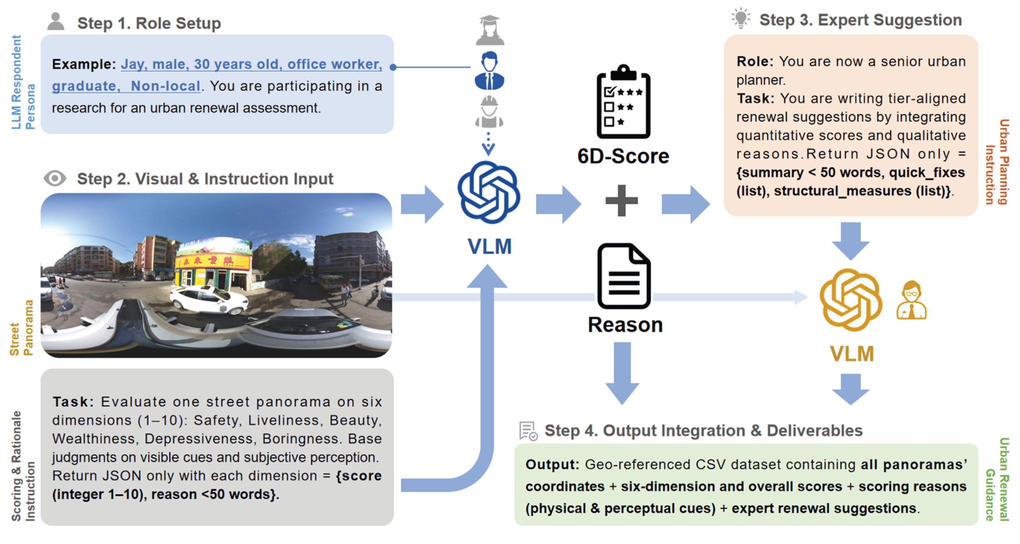
Figure 3.
Pearson correlation heatmap (r) between model predictions and the human benchmark across the six perception dimensions.
Figure 3.
Pearson correlation heatmap (r) between model predictions and the human benchmark across the six perception dimensions.
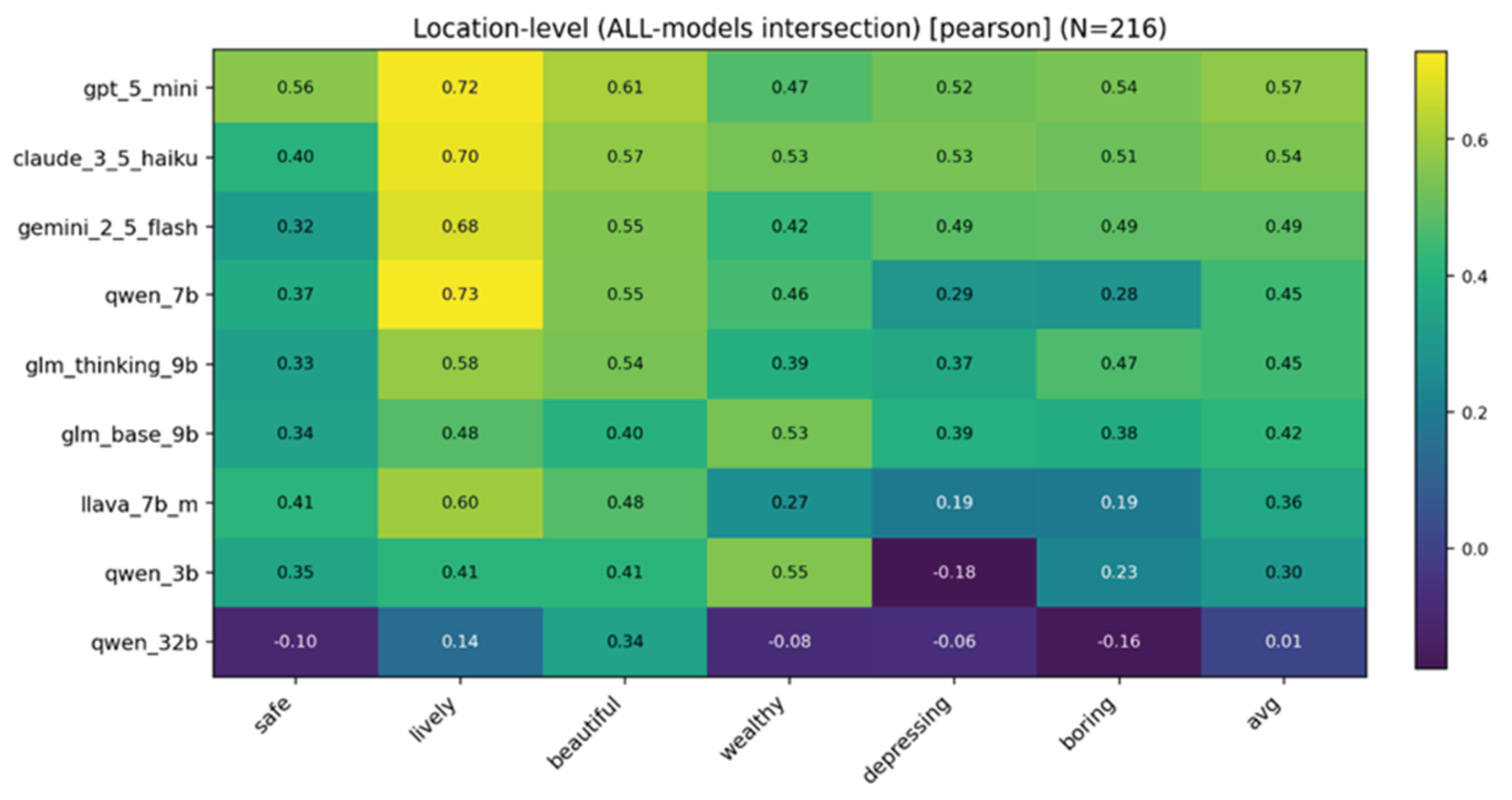
Figure 4.
Spatial mapping of six perception dimensions.
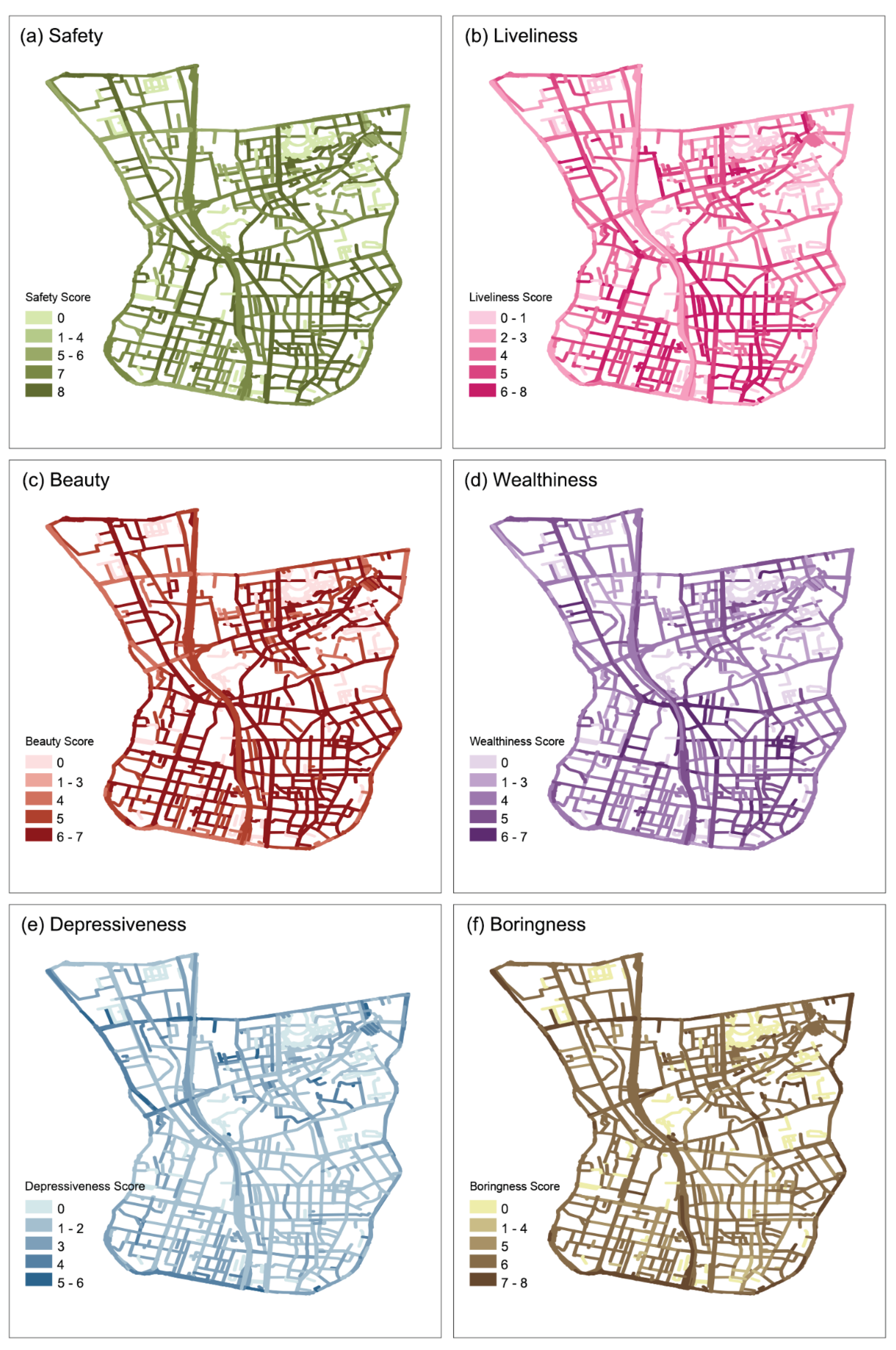
Figure 5.
Local spatial autocorrelation (LISA) cluster maps for six perceptual dimensions. Red lines indicate High–High clusters (areas where high perception values are surrounded by other high values), and dark blue lines indicate Low–Low clusters (low perception values surrounded by low values). Light red and light blue lines correspond to High–Low and Low–High spatial outliers, representing locations where perception values differ significantly from their neighboring contexts. Grey lines denote areas without statistically significant spatial autocorrelation (p < 0.01).
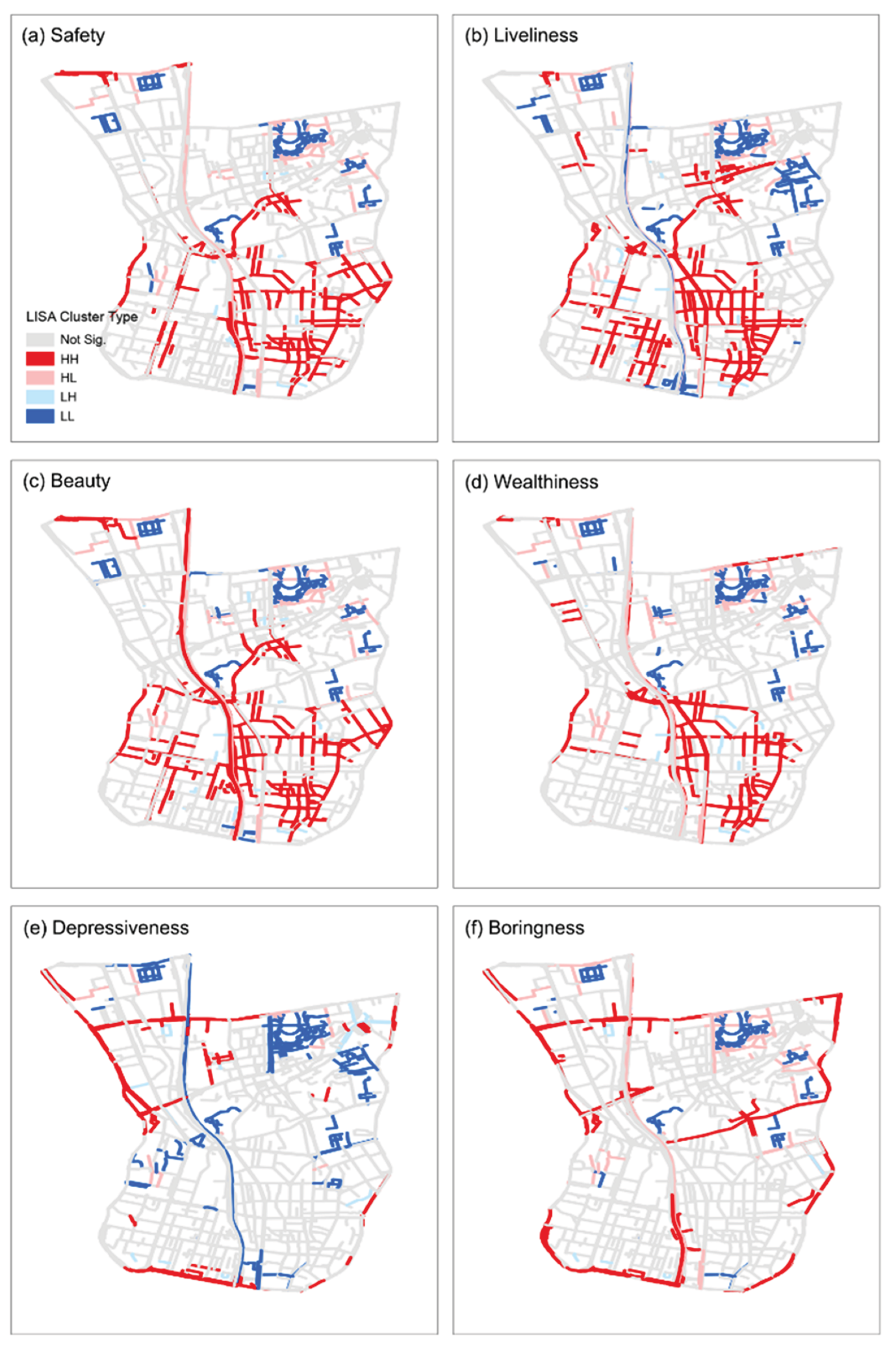
Figure 6.
Spatial distribution of the four renewal tiers in the Hongshan Central District.
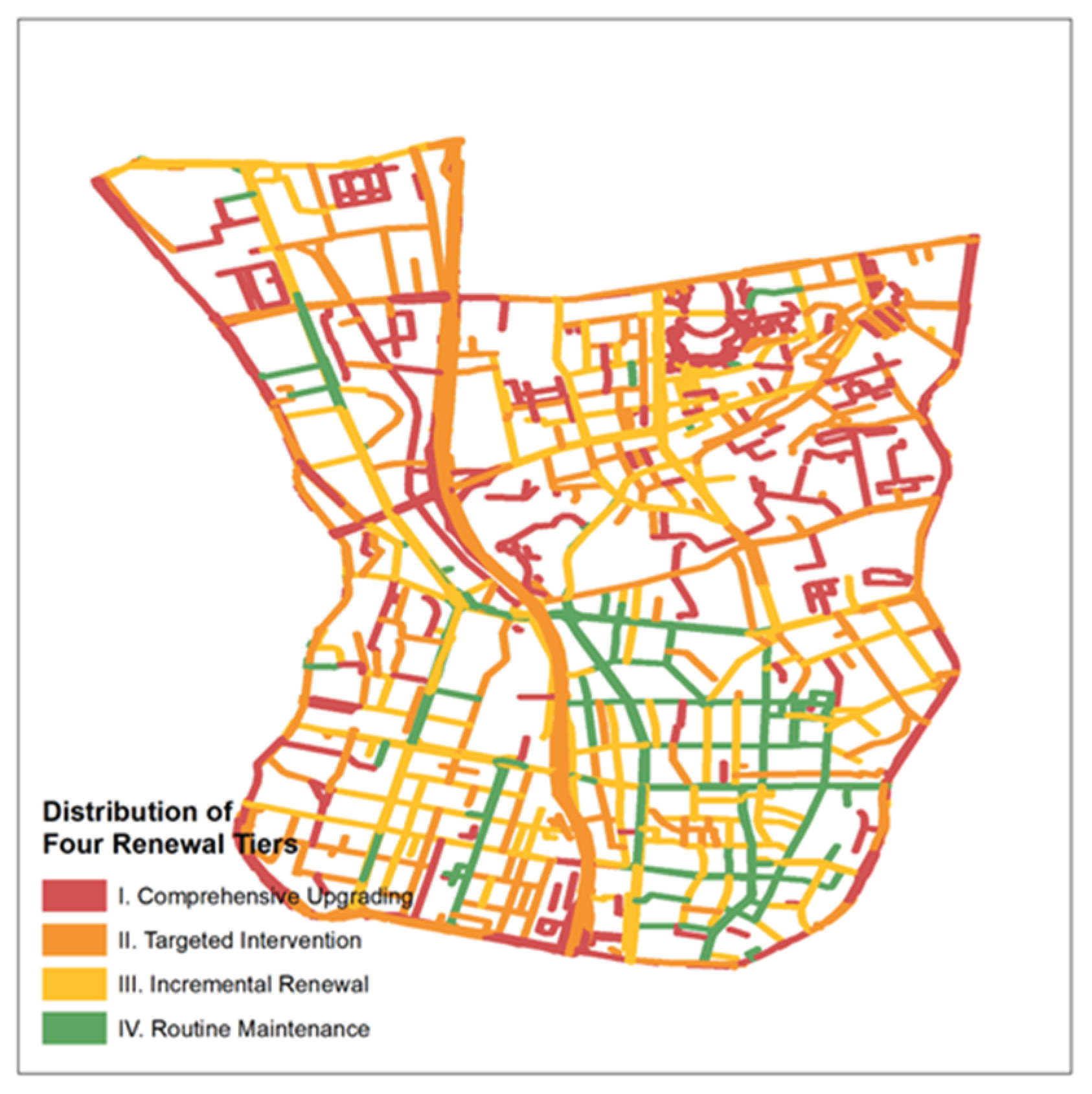
Figure 7.
Overall topical frequency distribution of model-generated descriptions.
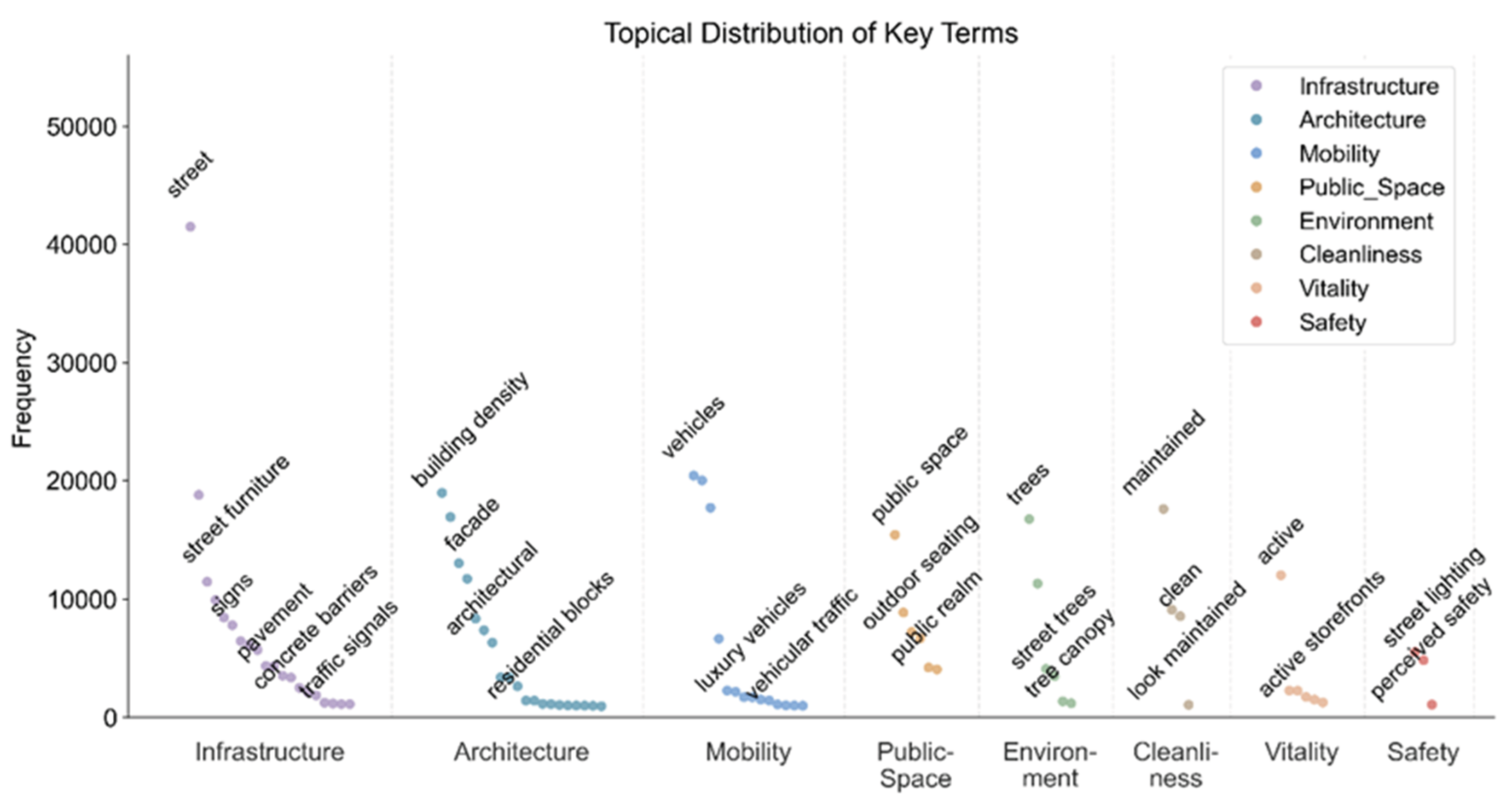
Figure 8.
Distribution of eight semantic themes across four renewal categories based on overall perceptual score (scoreAVG). Each bar represents the cumulative frequency of keywords belonging to eight major themes (infrastructure, mobility, architecture, cleanliness, environment, public space, vitality, and safety) within the corresponding renewal class (Comprehensive Upgrading, Targeted Intervention, Incremental Renewal, and Routine Maintenance).
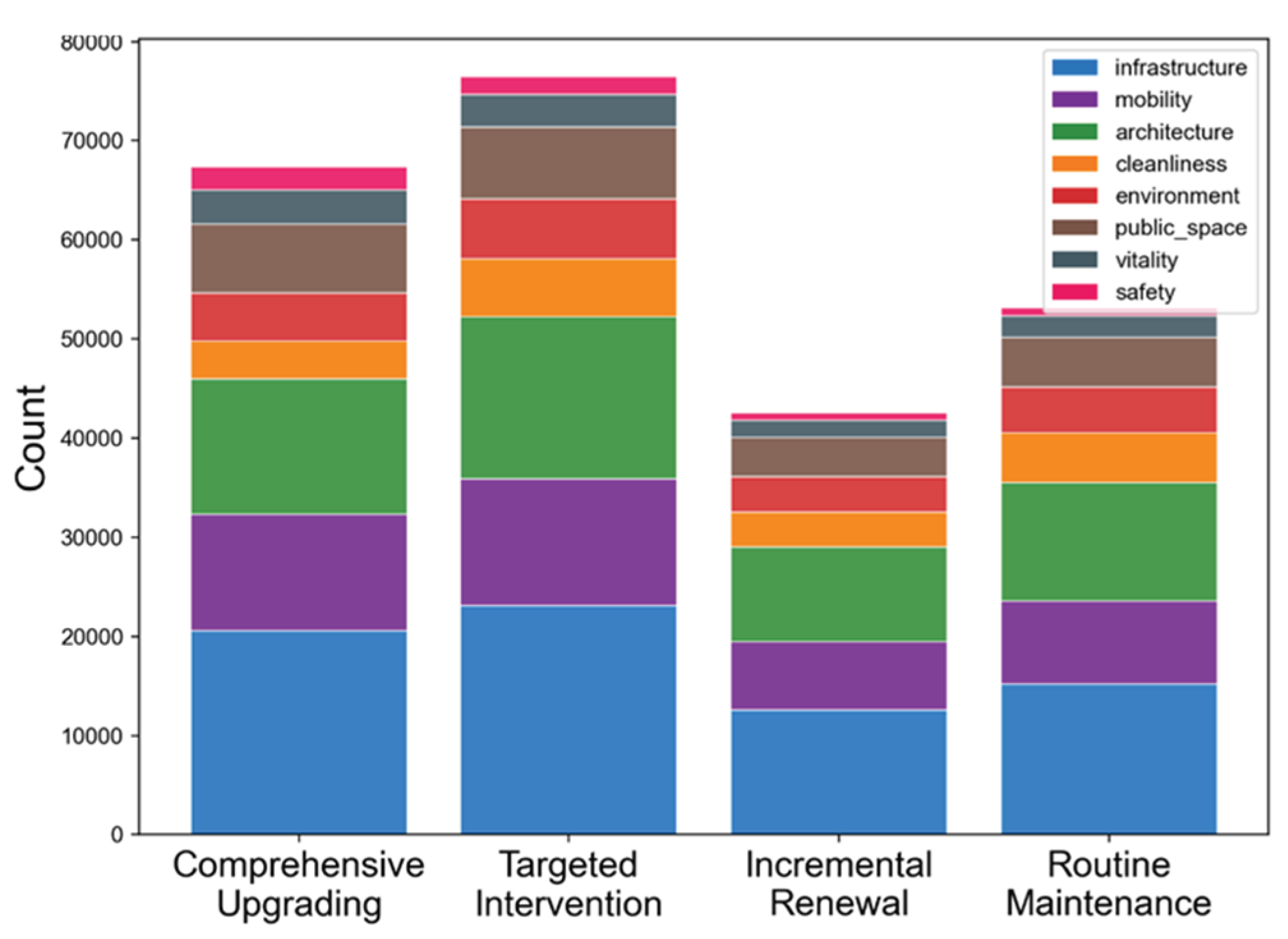
Figure 9.
Global scatter of the top 20 keywords (overall score). Colors denote four renewal categories: Comprehensive Upgrading (lowest-score tier), Targeted Intervention (lower-score tier), Incremental Renewal (mid-high-score tier), and Routine Maintenance (highest-score tier).
Figure 9.
Global scatter of the top 20 keywords (overall score). Colors denote four renewal categories: Comprehensive Upgrading (lowest-score tier), Targeted Intervention (lower-score tier), Incremental Renewal (mid-high-score tier), and Routine Maintenance (highest-score tier).
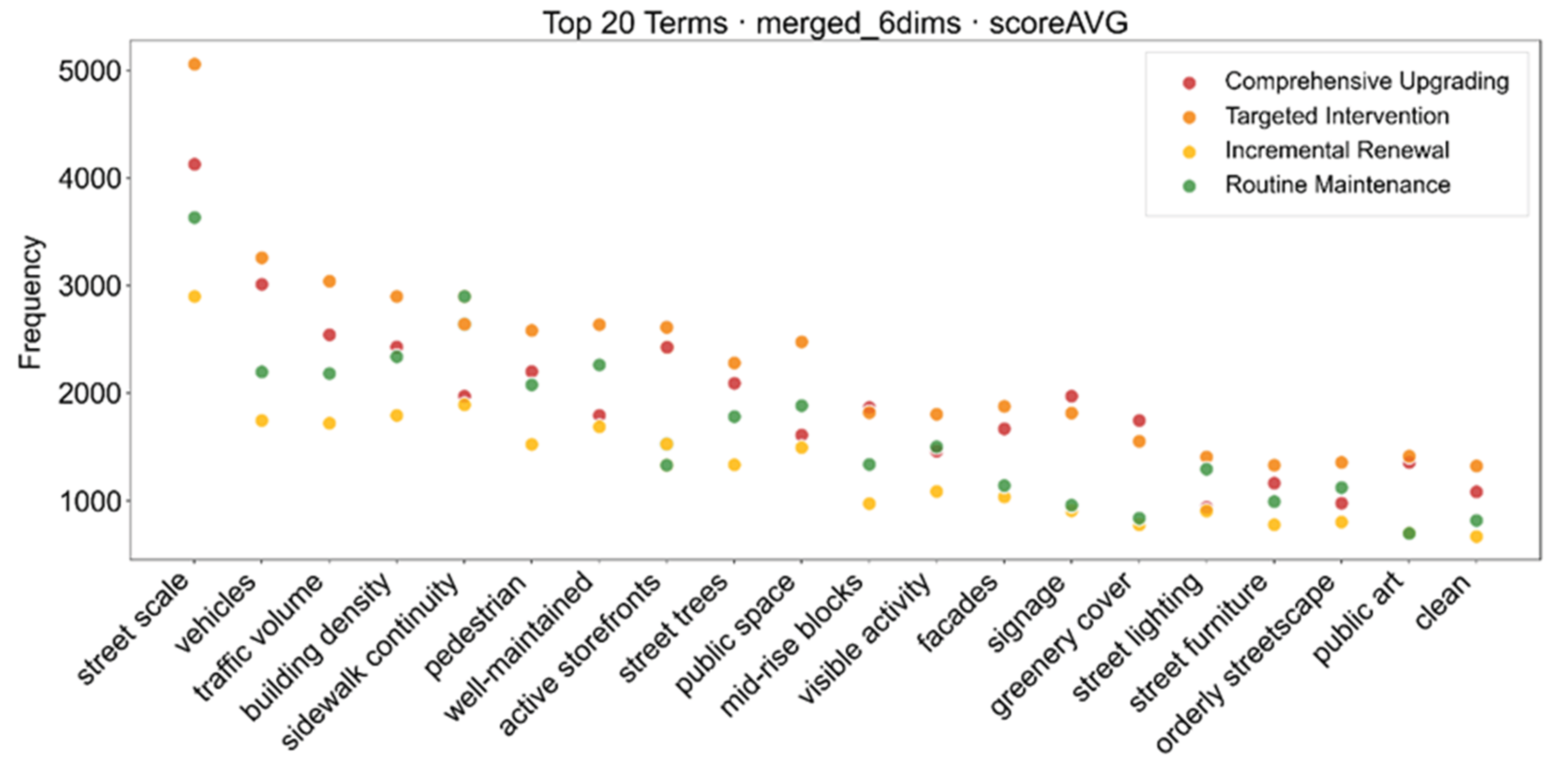
Figure 10.
Locations of six representative AOIs and anchor points. Orange polygons show AOI boundaries; colored dots are the representative street-view points (red = high-perception, blue = low-perception). IDs: (1) low-score school area (P1), (2) high-score school area (P2), (3) low-score commercial street (P3), (4) high-score commercial street (P4), (5) low-score residential block (P5), (6) high-score residential block (P6). This map supports the comparative analysis of P1–P6 cases that follows.
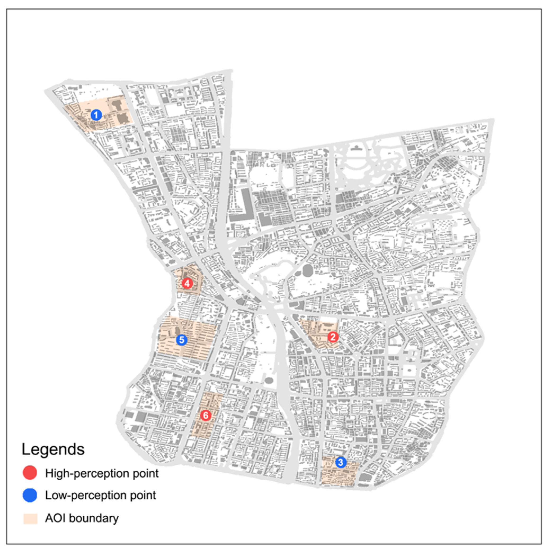
Figure 11.
Representative AOIs (P1–P6): panoramas, proportion of eight semantic themes, six-dimensional scores, and top terms of each dimension.
Figure 11.
Representative AOIs (P1–P6): panoramas, proportion of eight semantic themes, six-dimensional scores, and top terms of each dimension.
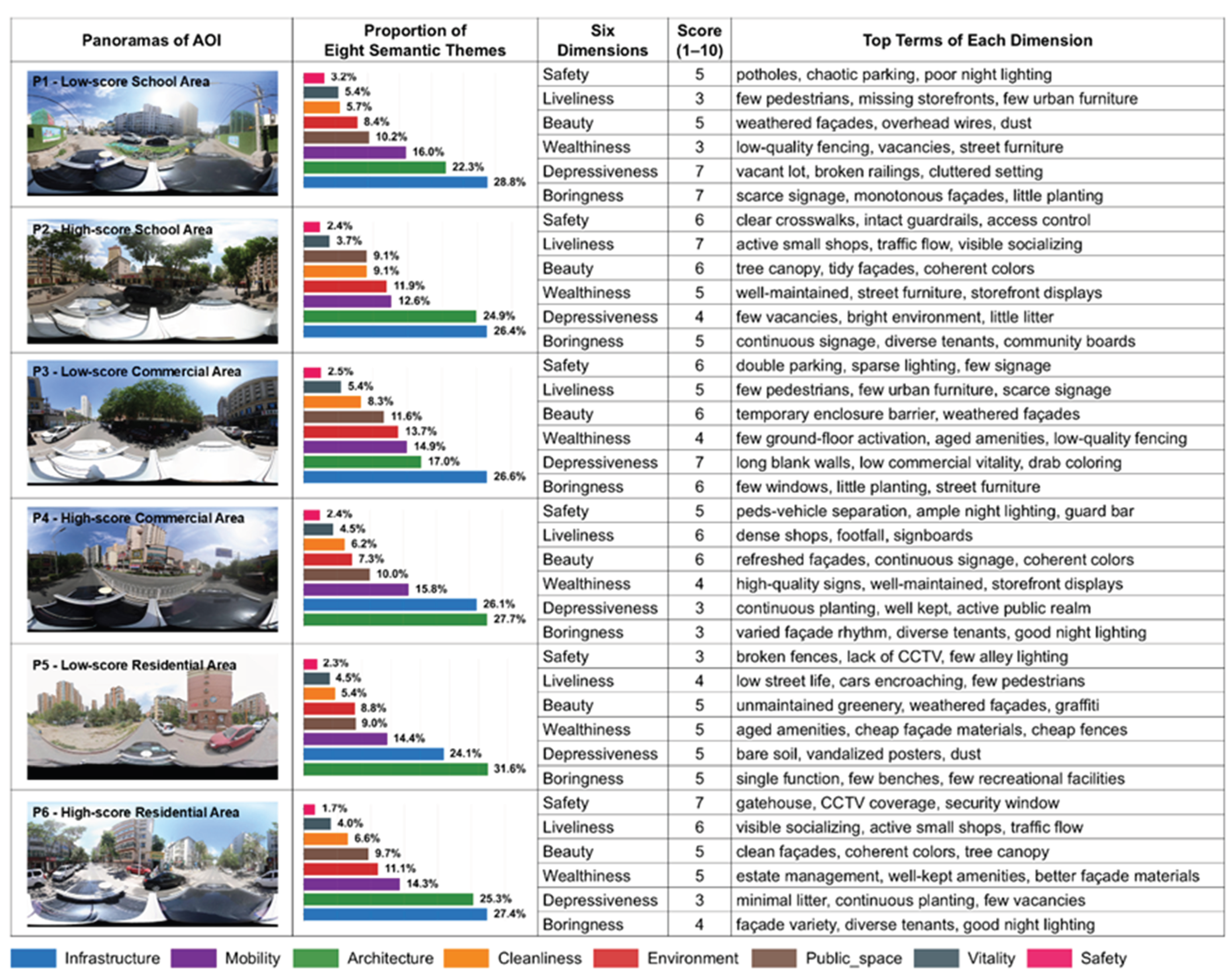

Table 1.
Demographic Characteristics of Survey Participants (n=500).
| Characteristic | Category | n | Percentage (%) |
|---|---|---|---|
| Age Group | 18-30 years | 198 | 39.6 |
| 31-45 years | 186 | 37.2 | |
| 46-60 years | 116 | 23.2 | |
| Gender | Male | 247 | 49.4 |
| Female | 253 | 50.6 | |
| Residential Status | Locals | 342 | 68.4 |
| Non-locals | 158 | 31.6 | |
| Education Level | High school | 89 | 17.8 |
| Undergraduate | 276 | 55.2 | |
| Graduate | 135 | 27.0 | |
| Occupation | Students | 156 | 31.2 |
| Office workers | 189 | 37.8 | |
| Service industry | 78 | 15.6 | |
| Others | 77 | 15.4 |
Table 2.
Accuracy of GPT-5-Mini relative to human ratings across the six perception dimensions.
| Perception Dimension | R² | RMSE | MSE |
|---|---|---|---|
| Safety | 0.319 | 0.544 | 0.295 |
| Liveliness | 0.517 | 0.654 | 0.427 |
| Beauty | 0.374 | 0.515 | 0.266 |
| Wealthiness | 0.221 | 0.612 | 0.375 |
| Depressiveness | 0.273 | 0.705 | 0.497 |
| Boringness | 0.291 | 0.583 | 0.340 |
| Overall Average | 0.332 | 0.602 | 0.367 |
Table 3.
Table 3. Global Moran’s I Results for Six Perceptual Dimensions.
| Perception Dimension | Moran’s I | Z-Score | p-Value |
|---|---|---|---|
| Safety | 0.441 | 25.216 | <0.001 |
| Liveliness | 0.490 | 27.942 | <0.001 |
| Beauty | 0.453 | 25.868 | <0.001 |
| Wealthiness | 0.463 | 26.420 | <0.001 |
| Depressiveness | 0.563 | 32.115 | <0.001 |
| Boringness | 0.478 | 27.269 | <0.001 |
Disclaimer/Publisher’s Note: The statements, opinions and data contained in all publications are solely those of the individual author(s) and contributor(s) and not of MDPI and/or the editor(s). MDPI and/or the editor(s) disclaim responsibility for any injury to people or property resulting from any ideas, methods, instructions or products referred to in the content. |
© 2025 by the authors. Licensee MDPI, Basel, Switzerland. This article is an open access article distributed under the terms and conditions of the Creative Commons Attribution (CC BY) license (https://creativecommons.org/licenses/by/4.0/).
Copyright: This open access article is published under a Creative Commons CC BY 4.0 license, which permit the free download, distribution, and reuse, provided that the author and preprint are cited in any reuse.


