
Submitted:
05 December 2025
Posted:
08 December 2025
You are already at the latest version
Abstract
An important part of geometry computations for synthetic aperture radar (SAR) carried on a satellite platform is to convert between the instrument-specific coordinate system and a geocentric coordinate system such as Cartesian Earth-centered, Earth-fixed (ECEF) coordinates, geodetic coordinates (latitude/longitude) or a projection of these. The solutions for points on or near ellipsoid height typically involves iteration over geodetic coordinates, which means performing the transformation from geodetic to ECEF and its 6 partial derivatives in every iteration step. We present a method for solving these equations in the satellite’s zero Doppler plane, which is typically used as coordinate plane for SAR systems with small squint angles. Solving the system in this plane means one of the constraints is satisfied implicitly, and allows solution which satisfies the other constraint (correct range from satellite) to be solved using a one-dimensional Newton method. The method is simple to implement, fast and accurate. For targets on the ellipsoid, the solution can be made as accurate as machine precision allows. For high-precision applications with targets at non-zero height above the ellipsoid, a small correction step is necessary, and we describe how to arrive at this step.
Keywords:
synthetic aperture radar
; satellite orbits
; geodesy
1. Background and Introduction
For a synthetic aperture radar (SAR) carried on a platform in motion, the natural coordinate axes for focused data are range (fast time: two-way pulse propagation time between instrument and target) and azimuth (slow time: a coordinate which gives the instrument’s position while pulsing. These two coordinates in isolation describe a sphere centered on the satellite. When data are focused (energy from a single target is concentrated to a point), we choose for a monostatic instrument with a small squint angle to always focus data to the zero-Doppler plane i.e. every target is focused at its point of shortest range. With this restriction, the pair of SAR coordinates describe a circle in the chosen plane.
For almost every other use, an object on or near the Earth’s surface will be placed in a coordinate system related to the Earth surface: Geodetic latitude and longitude, or any projection of these. The geodetic coordinates are related to a reference ellipsoid that approximates the Earth’s shape to a first degree, and a third coordinate is then the height relative to this ellipsoid. A further refinement of the Earth’s shape is the geoid which describes a surface everywhere normal to the local direction of gravity and coinciding with the mean sea level, and digital elevation models (DEMs) typically give height relative to the geoid. In this note we will only use height as relative to the ellipsoid.
For a surface described by a given ellipsoid and height, the circle described by the SAR coordinates will intersect this surface in zero, one or two points. Zero or one if the range is smaller than or exactly equal to the satellite’s height above the surface. The two points in the final case are solutions for a left- or right-looking instrument. The solutions on the far side of the Earth are mathematically valid, but not relevant here.
2. Transforming Between Cartesian and Geodetic Coordinates
Let = semimajor/semiminor axis of Earth’s ellipsoid; define geodetic latitude and longitude and ; ellipticity , and second ellipticity .
where is the local radius of curvature of the ellipsoid in the meridional plane.
For the inverse relation, longitude is simple (), but latitude is more involved. Closed-form solutions exist but don’t lend themselves to numerical use. Many iteration methods have been described in the literature [1] differing in their speed of convergence and their use of transcendental functions (sines and cosines). We found that the following formula due to Bowring [2] gives sufficient accuracy for the ellipsoids of interest to us in a single iteration:
where is the reduced (or elliptic) latitude of the point, (see Figure 1); and is the equatorial component of the position in the meridional plane, indicated by p in the figure. For a target on the ellipsoid, this formula gives latitude to within the representability of a double-precision floating-point number, radians. For a target at an altitude of 9000 m, the latitude coordinate is still within a m of the correct answer.
At satellite altitudes (1000 km) the error in latitude has increased to a few centimetres. If this is insufficient, a refined estimate of can be obtained as
Using this to compute a new value of gives answers that differ only in the last 1-2 bits of the numerical representation even at 1000 km.
Once geodetic latitude is known, height above the ellipsoid, when required, is given by
This expression evaluated in double precision gives height accurate to a few nm for a target from 0 and up to 9000 m height.
The complete set of range-Doppler equations is then as follows:
where r is range, () is the satellite’s position (velocity) at the given azimuth time, and is the solution (target position) being sought. The first equation states that the target must be at the correct range. The second equation states that the target must be in the correct plane. To use a different focus plane than the zero Doppler plane, replace the velocity vector with a normal vector to the chosen plane. The final equation requires the target to be at ellipsoid height. For height not at the ellipsoid, it takes a more complex form, as can be understood from Equation (6), but the solution can be found in an approach where this equation will be satisfied by construction, as explained in the next section.
3. Transformation from SAR Coordinates to Geodetic lat/lon
The traditional way of finding geodetic coordinates for given SAR coordinates is a 2-D Newton-Raphson search, using the fact that for a target in the zero-Doppler plane, the vector describing the target’s position relative to the satellite is perpendicular to the satellite’s velocity vector:
so the azimuth error is the value of this dot product. The error in range is the difference between the found and desired range. The Newton increment is then where is the Jacobian for the transformation from Cartesian geocentric coordinates to geodetic lat/lon, described in Section 2, above.
This method converges to an accuracy of 1 m in 5 or 6 iterations for a starting point within a hundred km or so. Such a starting point can be found by using the satellite’s position e.g. at the midpoint of a SAR scene and adding an offset of a few hundred km to the left or right.
A better starting point can be obtained by taking the satellite position for the given azimuth time, and using an approximate Earth radius and height to compute a triangle, using the third vertex of this triangle as the start point for the iteration, as illustrated in Figure 2. In this way, the method usually converges in 2 or 3 iterations.
3.1. Solutions in the Plane
While the 2D Newton method gives an answer to the desired accuracy and converges reasonably fast, it suffers by having to do all computations in three dimensions. A recent paper by Klein [3] gave closed-form expressions for the ellipse that results when intersecting a plane with an ellipsoid. When the target we seek lies on the ellipsoid, all quantities can be restricted to this plane. We should point out that the axes of this ellipse are in general not aligned with the axes of the ellipsoid. Here, we will describe the method in more detail, and show the accuracy of the approach for targets at all heights and along an entire representative SAR satellite orbit from Sentinel-1A. We will also discuss computational efficiency in the final section.
Following Klein’s description, we need a unit normal vector to the plane, for which we use the satellite’s unit velocity vector. We also need a vector for an arbitrary point in the intersection plane, for which we choose the satellite’s position. The unit vectors corresponding to the satellite’s right () and up () are rotated in the plane to form an orthonormal basis for the plane which also satisfies
where is the ordinary inner product of vectors in , and Klein’s and for the ellipsoid (used below) become and in our case.
The distance between the plane and the origin is given by , and we compute the centre of the ellipse by Klein’s equation /40/:
where
Using these results, and translating the coordinate system of the plane to place its origin at the centre of the intersection ellipse, the equation for the ellipse becomes
where the semiaxes are given by
with d given by Klein’s equation /25/ as .
A point with coordinates in the translated plane have ECEF coordinates in .
The axes of the intersection ellipse are in general not aligned with the axes of the ellipsoid. In Figure 3 we present the parameters of the intersection ellipses along an entire orbit of the Sentinel-1 satellite. The ellipses have a semimajor axis very close to the equatorial radius of Earth (). The semiminor axis varies between the equatorial and polar radii of Earth (panel 2). Hence, ellipticity and flattening of the intersection ellipse varies between those of the ellipsoid’s meridional ellipse, and zero (panel 3). The ellipse centre’s coordinates do not coincide with the centre of the ellipsoid, but the two are within a few km of each other (panel 4).
The intersection between an ellipse and a circle gives a quartic equation, and while there are closed-form solutions to these equations, iterative methods will again give answers to the required accuracy much more quickly and more easily. We use the reduced latitude in as iteration variable, and the difference from the desired range as the function whose root we’re trying to find:
where
and is the satellite’s coordinates in the system.
We can use the same kind of triangle equation to find a good starting point for this iteration. In practical tests, we converge to less than a in three iterations, and three iterations are completed in roughly half the time of a single iteration of the 2D Newton search.
3.2. Beyond the Plane: Nonzero Height
When we geolocate a target at nonzero height, we are still looking for a point strictly within the zero Doppler plane, but we have added two complexitites that were not present in the zero-height case:
- the point is no longer on the intersection ellipse, and
- the distance from the point to the ellipse is not the same as the distance from the point to the ellipsoid (the height which we’re interested in).
For an arbitrary ellipsoid and plane configuration, these problems are not easily tractable. In the context of a satellite in low Earth orbit, the following properties make our problem more tractable:
- The ellipsoid is close to spherical (for WGS-84, f = 1/298.257223563)
- The distance from the origin (centre of the Earth) to the zero Doppler plane is typically small relative to the Earth radius, i.e. a few km.
Hence, the intersection ellipse is almost exactly circular, and the zero Doppler plane and the local tangent plane are very nearly normal to each other.
In the 1D iteration described above, we use the ellipsoid with half-axes and instead of A and B. This is not exactly the curve where we’re looking for a solution, but the difference is nowhere greater than 1–2 centimetres for terrestrial targets, see Figure 4 and caption.
The iteration converges to within in range in three iterations, just as for the zero-height case.
The next approximation is we are now close enough to the sought coordinates that the surface normal to the ellipsoid which passes through the target is indistinguishable1 from the one computed in , the point we arrived at using the 1D iteration over the enlarged ellipse. It differs from the normal to the intersection ellipse through this point in the intersection plane, though, and the dot product between these two normal vectors gives the factor by which the height above the ellipsoid we have arrived at, , differs from the desired height, h:
While we could easily compute a new height and repeat the 1D Newton method, it turns out we are now close enough to the true solution that we can compute directly the 3D direction and step to arrive at the desired solution. The geometry is shown in Figure 5.
The point we arrived at, , lies in the correct plane, has correct range to the satellite, it has a height very close to h above the ellipse, and height above the ellipsoid. Since , the step direction is perpendicular to the relative position between satellite and , and inside the zero Doppler plane, which means it can be expressed by way of the unit vector . In the plane containing the vector and the surface normal to the ellipsoid that passes through the desired point P, we can easily see that the step size is , and , i.e.
The unit normal vectors and are given directly by their foot point coordinates in the and coordinates, respectively:
We have now obtained the 3D coordinates of the target in geocentric Cartesian coordinates. For some applications, this is the desired result. If geodetic coordinates are required, the transformation described in Section 2 above can be applied.
4. Accuracy of the Results
For targets at ellipsoid height, the described method (including choice of iteration start point) gives answers limited by floating-point accuracy in three iterations.
For targets at any interesting nonzero height, we arrive at a solution which is at correct range to within a few tens of micrometers, and similarly not out of the zero-Doppler plane by an amount larger than this. The correction (18) does not change the range or out-of-plane errors appreciably.
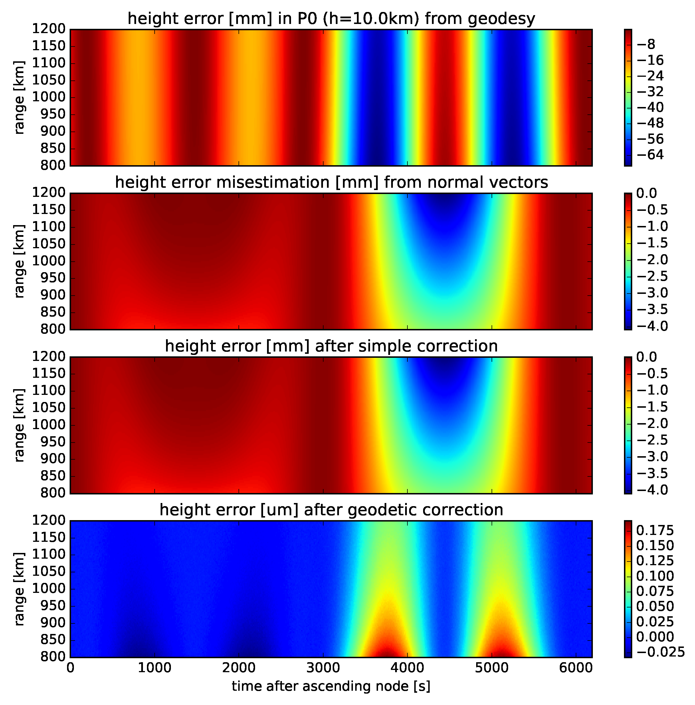
The error that could potentially remain affects the precise vertical and horizontal coordinates of the target, and ranges from less than a millimetre to a few millimetres, as seen in the third panel of Figure 6. This error is much smaller than the absolute accuracy of orbital information, and also of the digital elevation models. Therefore, it has no practical consequence.
It is of academic interest to remove even this tiny residual error. The only source of the error is the misestimation of the height of point above the ellipsoid. Using the geodetic formula for height (6) removes the error completely, as seen in the final panel of Figure 6, at the cost of one conversion from Cartesian to geodetic coordinates.
A less computationally expensive possibility is to model this misestimation as a function of ellipticity and target height. All terrestric targets () of interest to SAR are close enough to the ellipsoid that errors scale linearly with altitude, as shown by Figure 4. This means that curves such as those in the figure can be precomputed for a single height and for ellipticities between the limits seen in Figure 3. A correction to can be interpolated from these curves by latitude and ellipticity, and scaled by the height.
5. Efficiency Considerations
Most end products of SAR data for Earth observation will end up being geolocalized ([5] Section 1.5). Especially for full-resolution products this is a computationally expensive operation, and improving the efficiency of this conversion is valuable to reduce this cost. To see the expected impact of this method we must try to count fundamental operations, since benchmarks in a high-level programming language can be distorted by factors having little to do with the properties of the algorithms themselves.
The performance baseline is the 2D Newton-Raphson iteration described in Section 3, which we will call geodetic iteration in the following. We will not count the time spent finding a candidate position, since that is comparable in the two algorithms. We will also disregard time spent propagating or interpolating statevectors for the platform’s trajectory, since these costs are equal for the two algorithms.
Each geodetic iteration involves the evaluation of the dot product (8), which is done in ECEF, so the coordinates must be converted according to Equations (1)–(3), along with their partial derivatives with regard to latitude and longitude, and some other bookkeeping operations. If care is taken to compute sines, cosines and other common terms only once in each iteration, this involves a total of 4 trigonometric functions, 2 square root, 51 multiplications, 7 divisions, and 46 additions or subtractions. The cost of comparing the metric to a threshold is not counted,
The in-plane solution has some setup costs associated with the computation of the intersection ellipse and its basis vectors. We shall count up these costs, but we will point out that these results are common to all points with a common azimuth coordinate, so the cost can be divided over hundreds or thousands of points in typical cases. Computing the intersection ellipse, its basis and parameters (up to but not including Equation (13)) involves 3 trigonometric functions, 4 square roots, 116 multiplications, 11 divisions, and 45 additions or subtractions.
The computation necessary for each iteration and each point (Equations (13)–(16)) now consist of 2 trigonometric functions 11 multiplications, 1 division and 6 additions/subtractions.
When height is not zero, the extra step to correct for out-of-plane height error involves 28 multiplications, 15 divisions, 17 additions and 3 square roots per point
The relative costs of the different types of operations depend on the details of the computer hardware used, but for a current high-performance computer the cost of operations as multiples of the time spent on a single addition or subtraction we will use the factors 3 (multiplications), 5 (divisions), 7 (square roots) and 13 (trigonometric functions).
With these relative costs, the cost per geodetic iteration is roughly 300 units, while the in-plane method costs 70 units per iteration, roughly a factor of 4 improvement.
References
- Burtch, R. A Comparison of Methods used in Rectangular to Geodetic Coordinate Transformations. ACSM Annual Conference and Technology Exhibition, 2006; pp. 1–25. [Google Scholar]
- Bowring, B. R. TRANSFORMATION FROM SPATIAL TO GEOGRAPHICAL COORDINATES. Survey Review 1976, 23(181), 323–327. [Google Scholar] [CrossRef]
- Klein, P. P. On the Ellipsoid and Plane Intersection Equation. Applied Mathematics 2012, 2012, 1634–1640. [Google Scholar] [CrossRef]
- Grydeland, T.; Larsen, Y. Beyond Plane Sailing: Solving the Range-Doppler equations in a reduced geometry. Proceedings of EUSAR 2018: 12th European Conference on Synthetic Aperture Radar, 2018. [Google Scholar]
- Franceschetti, G.; Lanari, R. Synthetic Aperture Radar Processing; CRC Press, 1999. [Google Scholar]
| 1 | The dot product between this normal vector and the one computed at the foot point of the most carefully corrected process described herein differs from 1 in the 11th digit. |
Figure 1.
Figure showing the definition of geodetic latitude, , and reduced latitude, , in the meridional plane. Illustration by Peter Mercator, placed in the public domain by the creator.
Figure 1.
Figure showing the definition of geodetic latitude, , and reduced latitude, , in the meridional plane. Illustration by Peter Mercator, placed in the public domain by the creator.
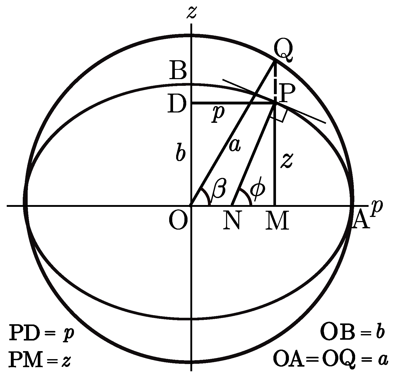
Figure 2.
An improved initial guess for the target’s position. The side lenghts of the triangle are known: The satellite’s position relative to the Earth centre is known, the range is specified, and the target’s height is known to good accuracy with very rough knowledge of latitude. From these distances, the angle can be computed. The heights of the satellite and target above the ellipsoid are exaggerated.
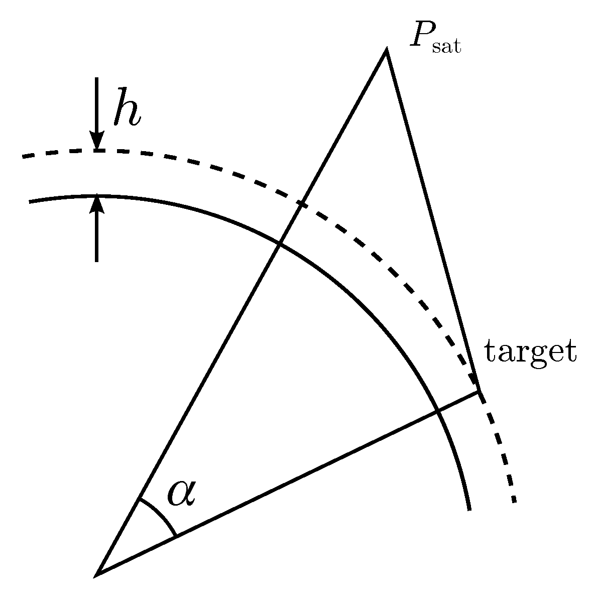
Figure 3.
Parameters of the intersection ellipses for a full Sentinel-1 orbit. The x axis shows seconds since the ascending node in all panels. The first panel shows the angle through which the base had to be rotated to make the basis vectors line up with the axes of the ellipse. This figure mostly reflects the satellite’s position in its orbit. The second panel shows how the semiaxes, as computed by Equations (12), relate to the Earth’s equatorial radius. The deviations are exaggerated by a factor 1000 for the semi-major axis which only varies by a few metres. The semi-minor axis varies between the Earth’s polar and equatorial radii in reflection of the angle of the zero-Doppler plane. The third panel shows the ellipse parameters flattening () and ellipticity squared () for the intersection ellipses. As expected, and consistent with the semiaxes variations, the values range between those of the Earth’s meridional ellipse and a circle (). The final panel shows the coordinates of the intersection ellipse’s centre point, as computed by Equation (10). The point is within a few kilometres of the Earth centre.
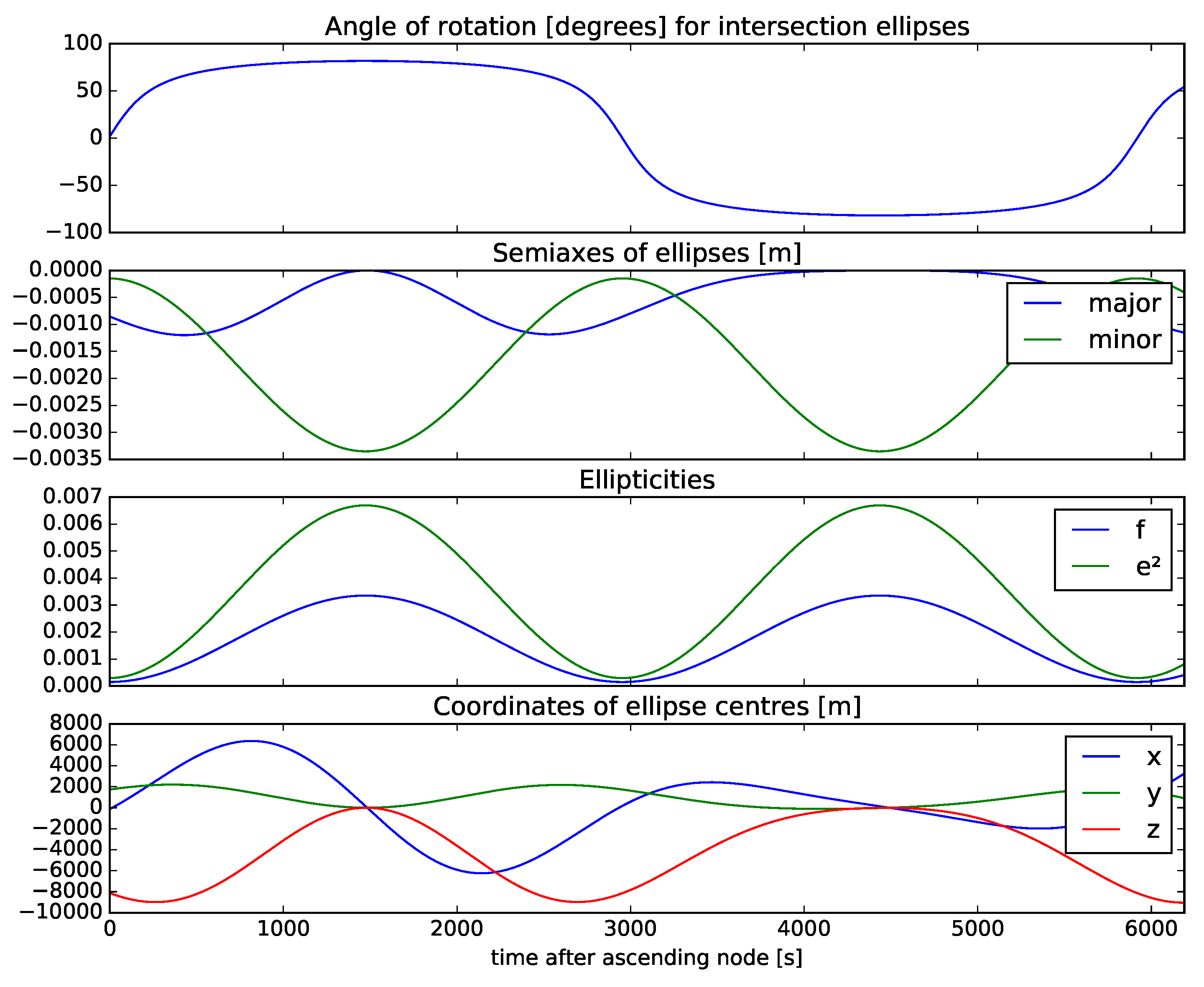
Figure 4.
Increasing the radius of a circle by h results in a new curve where every point is at a distance h from the original circle. For an ellipse, increasing both semiaxes with h results in a new curve which is at distance h for points on the axes, but slightly closer at intermediate latitudes. Plotted here is the size of this offset relative to the nominal heigh, in units of millimetres per kilometer of height, for a meridional ellipse of WGS-84, and for various heights h from 1 to 100 km. As can be seen from Figure 3, the intersection ellipse is nowhere more eccentric than the meridional ellipse, so these curves represent an upper bound on the contribution to height misestimation from this effect.
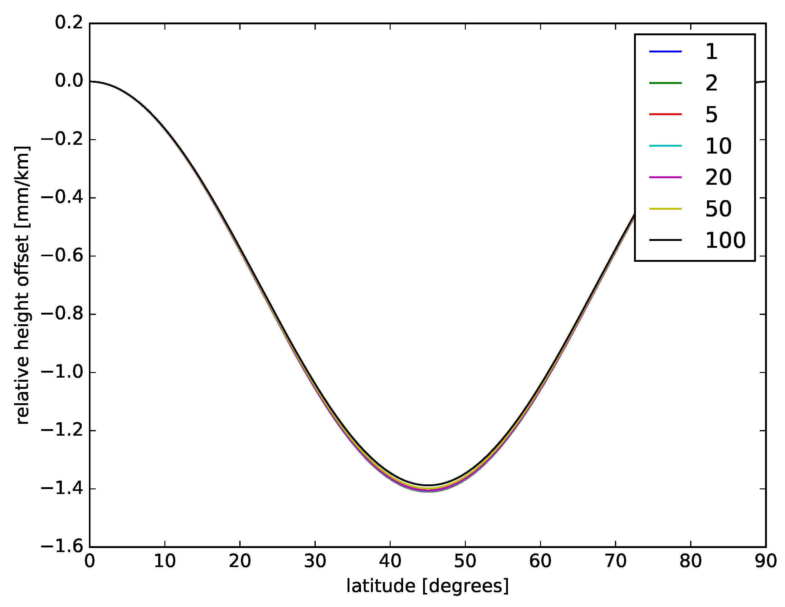
Figure 5.
How we arrive at the step size. The plane of the illustration is not exactly the zero Doppler plane, but the points P and and surface normal vector all lie in the illustration plane. The upper and lower nearly-horizontal curves represent the enlarged ellipse used to find the approximate solution and the line drawn by its foot points on the ellipsoid projected back into the illustration plane, respectively. In practical terms the distances in this illustration are so small that this is a line with constant offset from the enlarged ellipse, and both ellipses are well represented as straight lines within the figure. The curvature of the ellipses is highly exaggerated in the illustration.
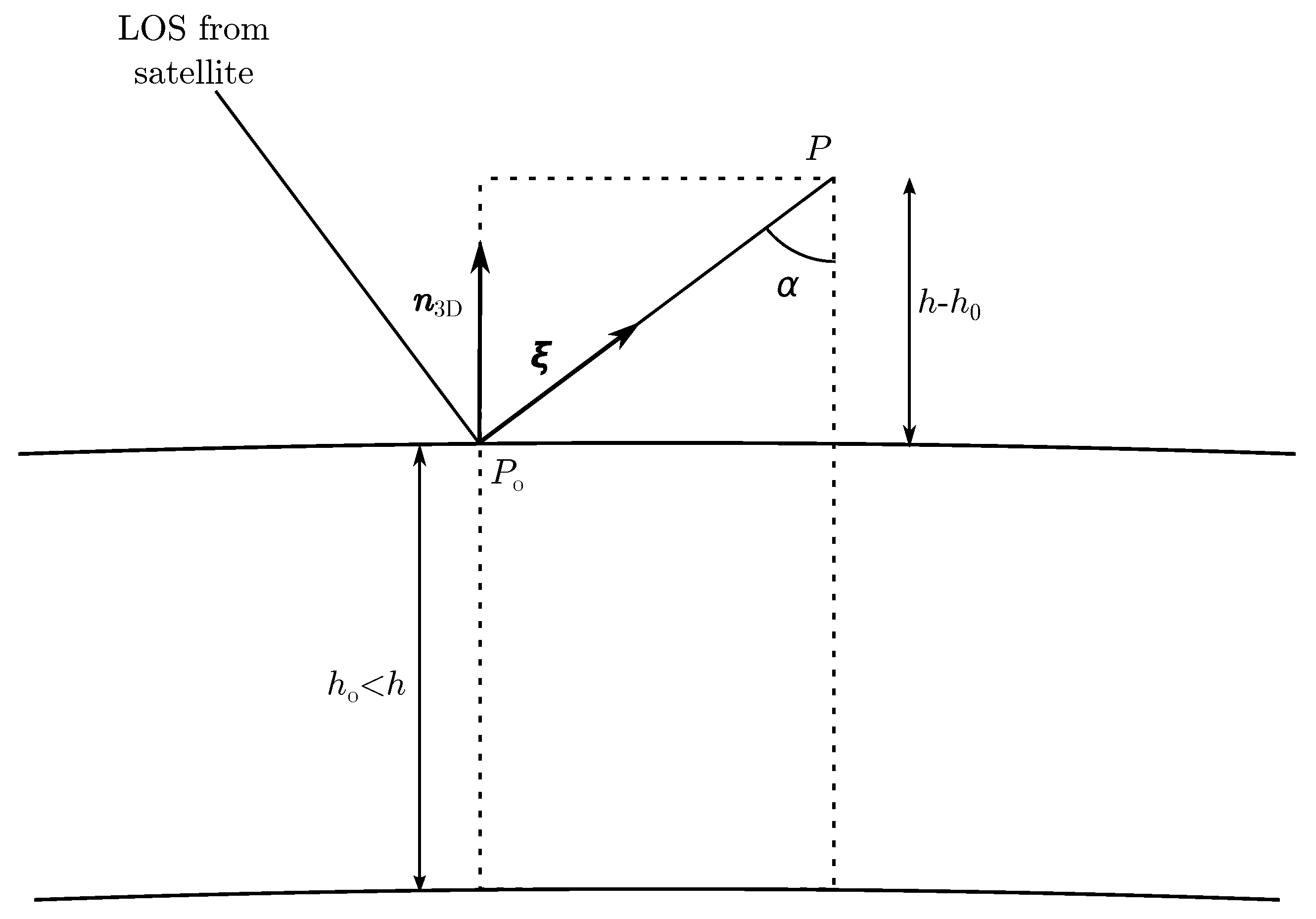
Figure 6.
Height errors for targets at 10 km altitude for the same orbit shown in Figure 3 as functions of seconds after ascending node (x) and range in kilometres (y). The first panel shows the difference between the height of the point above the ellipsoid as given by Equation (6) and the 10 km height sought, in units of millimetres. The second panel shows by how much the height error described by Equation (17) misestimates the height error in the first panel. The height error is mostly determined by latitude. It is near zero near the equator and the poles, and largest at intermediate latitudes. The misestimation is only noticeable when height error and intersection ellipse eccentricity interact. The third panel shows the height error that remains after the correction step illustrated in Figure 5 has been applied. The fact that this error is indistinguishable from the error misestimation in the previous panel indicates that the step is correctly computed and applied. This is also demonstrated by the final panel, where the height error after correction step is also shown, but when the step was scaled by and was computed using (6). Notice that in this panel, the error is in units of micrometres.
Disclaimer/Publisher’s Note: The statements, opinions and data contained in all publications are solely those of the individual author(s) and contributor(s) and not of MDPI and/or the editor(s). MDPI and/or the editor(s) disclaim responsibility for any injury to people or property resulting from any ideas, methods, instructions or products referred to in the content. |
© 2025 by the authors. Licensee MDPI, Basel, Switzerland. This article is an open access article distributed under the terms and conditions of the Creative Commons Attribution (CC BY) license (http://creativecommons.org/licenses/by/4.0/).
Copyright: This open access article is published under a Creative Commons CC BY 4.0 license, which permit the free download, distribution, and reuse, provided that the author and preprint are cited in any reuse.


