Submitted:
06 December 2025
Posted:
08 December 2025
You are already at the latest version
Abstract
Accurate forecasting of wind power is essential for maintaining the stability and efficiency of power networks as renewable energy sources become more integrated. This study proposes a multilevel spatial-temporal graph convolution network (MLAGCN) for wind power forecasting. The framework combines a multilevel adaptive graph convolution (MLAGC) and a lightweight temporal transformer (LWTT) to jointly model complex spatial-temporal relationships in wind power data. MLAGC is constructed using three adaptive graphs: a local-aware graph, a global-aware graph, and a structure-aware graph. These components form a flexible graph structure that effectively represents dynamic spatial interactions while LWTT learns short- and long-term sequential patterns. Experiments on real wind farm datasets demonstrated that the proposed model outperforms existing baselines. The model achieved an improved prediction accuracy and generalization, as indicated by a lower score of 43.44, mean absolute error (38.83), root mean square error (48.05) and a forecast loss of 0.22. These results demonstrates the effectiveness of temporal modeling and multilevel attention-based adaptive graph learning for high-resolution wind power forecasting.
Keywords:
wind power forecasting
; spatiotemporal modeling
; adaptive graph convolution networks
; temporal transformer
; attention mechanisms
; renewable energy prediction
; wind farm spatiotemporal correlation
1. Introduction
The demand for precise wind power forecasting (WPF) has increased due to the growing emphasis on sustainable energy sources. The inherent unpredictability and fluctuation of wind energy pose operational challenges for grid stability, energy dispatching, and cost efficiency as it becomes increasingly integrated into global electrical systems. To balance power generation and consumption, reduce dependency on reserve capabilities, and facilitate the effective integration of wind energy into the power system, precise WPF is essential [1,2].
Wind power forecasting (WPF) research has utilized a range of modeling paradigms, including statistical techniques, physics-based simulations, and, more recently, data-driven machine learning (ML) and deep learning (DL) models. Traditional methods such as Kalman filters and autoregressive integrated moving average (ARIMA) models achieved initial success in high-resolution, real-time forecasting but exhibited limitations in scalability and reliability [3]. In recent years, ensemble learning approaches and neural networks have gained prominence for their ability to model complex and nonlinear temporal patterns [4].
Graph-based learning constitutes a significant advancement in modeling spatiotemporal dependencies in wind power forecasting. The spatial distribution of wind farms necessitates models that can encode inter-turbine correlations based on topological or physical proximity, a capability provided by graph neural networks (GNNs) [5,6]. However, static graph architectures often fail to capture dynamic dependencies, particularly under rapidly changing climatic conditions. This limitation has led to the development of adaptive or attention-based graph construction algorithms that learn dynamic edge weights to reflect temporal variations in inter-node influence [7].
Graph Convolutional Networks (GCNs) have been utilized in recent studies for wind forecasting. Liu et al. [8] introduced a spatiotemporal GCN that incorporates temporal attention and spatial structure for wind power prediction. Song et al. [5] developed an end-to-end GCN-based approach that learns robust spatial representations using multi-resolution convolutional neural networks (CNN). However, many of these models rely on fixed graph topologies, which restrict their adaptability to evolving wind field dynamics.
The incorporation of attention mechanisms into graph structures has substantially improved WPF models. These mechanisms increase model responsiveness to evolving wind patterns by enabling the network to prioritize dynamically relevant turbines. The KDD Cup 2022 spatial dynamic wind power forecasting (SDWPF) challenge [7] highlighted this advancement by promoting adaptive modeling approaches and introducing the SDWPF dataset, which features comprehensive spatiotemporal properties. Methods that combined transformer-based architectures with global and local attention mechanisms, such as the graph spatial attention transformer (GSAT) [9], achieved state-of-the-art performance on this benchmark.
Temporal modeling remains a critical component of wind power forecasting. Although recurrent neural networks (RNNs) and their variants, such as long short-term memory (LSTM) and gated recurrent units (GRU), are widely used, they often fail to capture long-range dependencies. Recently, transformer models have been applied to wind and solar forecasting due to their self-attention mechanisms, which offer a scalable solution [10,11]. These models offer a robust framework for modeling complex spatiotemporal correlations in wind power data, particularly when combined with adaptive spatial modeling.
This study introduces a framework that simultaneously models long-range temporal dynamics and dynamic spatial relationships by integrating multilevel adaptive graph convolution (MLAGC) with a temporal transformer (LWTT) inspired by [12]. The framework employs multi-level attention mechanisms, including self-attention for dynamic topology refinement, global channel attention for wide-area dependencies, and local channel attention for short-range correlations, to adaptively construct the graph structure. Evaluation on SDWPF datasets demonstrates that the proposed model surpasses existing approaches across multiple performance metrics. In summary, the contributions of this work are as follows:
- A Novel Adaptive Graph Convolutional Network (MLAGCN) Framework: The paper introduces a new spatial-temporal forecasting framework that combines an adaptive graph convolution (MLAGC) with a temporal transformer (LWTT). Unlike static graph models, the MLAGCN dynamically learns the spatial structure of wind turbines using multi-level attention mechanisms, enabling it to model non-stationary spatial interactions across a wind farm.
- A Multi-Level Attention Mechanism for Graph Construction. The model constructs a flexible graph using three distinct attention mechanisms: self-attention for learning dynamic global topology, global channel attention for modeling long-range dependencies, and local channel attention for capturing short-range spatial correlations. This multi-attention design allows the model to flexibly adapt to both local turbine dynamics and global meteorological influences.
- A Temporal Transformer Module for Long-Range Sequence Modeling. A transformer-based temporal module (LWTT) is integrated to model long-term temporal dependencies in wind power data. This addresses the limitations of traditional RNN-based approaches (e.g., GRU, LSTM) that struggle with capturing long-horizon temporal patterns.
Figure 1.
The overall architecture of our proposed MLAGCN.

Figure 2.
Light-weight Transformer architecture.
2. Related Works
2.1. Statistical-Based WPF
Early research mainly employed statistical methods to model weather data and predict wind power. Wind speed was initially identified as the most direct influencing factor for wind power prediction. Brown et al. [13] developed an autoregressive moving average (ARMA) model to predict wind speed, utilizing features such as autocorrelation and non-stationary behavior during nighttime. Subsequently, wind power was formulated as a function of wind speed, enabling direct estimation through transformations of wind speed data. The strong correlation between wind speed and wind power has led to the development of various methods for predicting wind speed. For instance, Firat et al. [14] applied independent component analysis (ICA) to predict wind speed data, while Mohandes et al. [15] utilized support vector machines (SVMs) for wind speed modeling. Additional factors, including geographic location and wind direction, also influence wind power. Alexiadis et al. [16] examined the spatial correlation of wind speeds and developed a statistical learning model for wind power forecasting. Sideratos et al. [3] combined historical wind farm power data with forecasts of wind speed and direction to propose an advanced statistical method for wind power forecasting. Despite extensive research on statistical methods for wind power prediction, substantial uncertainties in weather data, particularly wind speed, can undermine the reliability of both linear and nonlinear statistical models. These methods are generally limited to short-term predictions and are less effective for long-term forecasting. To address this limitation, more sophisticated statistical models have been introduced. Ahmadi [17] developed an XGBoost model, demonstrating that tree-based models can effectively predict long-term wind power, especially across diverse geographical locations. Based on these findings, WPF methods can be broadly categorized into classical statistical approaches and machine learning or deep learning techniques.
2.2. Deep Learning-Based WPF
Wang et al. [18] developed a wind power prediction framework that utilizes a convolutional neural network (CNN) and a wavelet transform. Experimental results indicate that this model is robust to noisy data and performs competitively on multiple real wind farm datasets. Song et al. [19] introduced a combined model based on a generalized regression neural network (GRNN). Yu et al. enhanced a long short-term memory (LSTM) model and applied spectral clustering to optimize forecasting performance. In recent years, the transformer model [20] has achieved notable success in long-term sequence prediction tasks. This success has led to the development of several variants. Informer [21] enhanced the self-attention mechanism to more effectively capture long-range dependencies. Autoformer [22] introduced a decomposition structure that enables effective modeling of complex time series, outperforming other methods in long-range forecasting tasks. Similarly, FEDformer [23] combined the transformer with seasonal-trend decomposition to capture both global and detailed time series information. Despite these advancements, comprehensive studies of transformer models and their variants in wind power prediction remain limited. The demonstrated effectiveness of transformers in graph modeling highlights their potential for wind power forecasting.
More recently, studies have increasingly adopted graph convolutional networks (GCNs) to improve wind power forecasting by modeling spatial dependencies among turbines. Multi-graph approaches have been proposed to capture correlations from different perspectives, such as geographical distance, statistical similarity, or fluctuation patterns, as seen in [24], who integrate spatio-temporal attention with four complementary graph structures. Other works incorporate physical interactions, such as blockage and wake effects, into the graph topology to better reflect turbine-to-turbine interactions [25]. Works like [26,27] demonstrated the advantages of graph-based spatial modeling for large wind farms. However, existing methods often rely on single-perspective graphs or complex multi-graph ensembles, leaving room for more unified and adaptive architectures that can capture spatial relations at multiple levels. In contrast, our method introduces a unified multilevel adaptive graph that jointly models local, global, and structure-aware dependencies within a single framework, which allows the model to learn fine-grained turbine-specific dependencies and broad spatial patterns simultaneously, without the overhead of manually engineered multi-graph combinations.
3. Methodology
3.1. Problem Formulation
A wind farm consists of N wind turbines situated within a specified geographical area. Each wind turbine independently generates electrical power. The Supervisory Control and Data Acquisition (SCADA) system records the operational status and power generation of each turbine at fixed time intervals. Let denote the observation matrix at time t, where N is the number of turbines and F is the feature dimension (e.g., wind speed, pitch angle, reactive power, active power). The sequence of observations over a historical window of length T is represented as
Wind power forecasting aims to estimate the active power output for all turbines in the wind farm over a future period of P time steps, based on historical data. The task is to determine a mapping function such that
represents the predicted active power output for all turbines at the forecasting horizon , where ranges from 1 to P.
A primary challenge in wind power generation is the presence of strong temporal dependencies resulting from evolving weather patterns and spatial correlations arising from similar wind flows affecting neighboring turbines. Additionally, wind power generation is subject to considerable stochastic uncertainty. Therefore, the objective is to develop a model that effectively captures these spatial-temporal dynamics to enable reliable multi-step forecasting.
3.2. Data Preprocessing
The Baidu KDD Cup 2022 challenge released a raw Supervisory Control and Data Acquisition (SCADA) dataset that includes meteorological variables such as wind speed, wind direction, and temperature, as well as turbine operational states including pitch angles, nacelle direction, and reactive power [7,26]. Auxiliary identifiers, including time, day, and turbine identification number, are also provided. The dataset comprises 4,727,520 records across 13 columns, collected from 134 turbines at 10-minute intervals over 245 days. These measurements frequently contain noise, redundancy, and missing values, which can reduce forecasting accuracy. To mitigate these issues, systematic preprocessing steps were implemented, including data cleaning, normalization, and feature refinement. The SDWPF dataset, derived from the Baidu KDD Cup 2022, is publicly available and originates from SCADA systems monitoring wind turbines at a wind farm operated by Longyuan Power Group [28]. The dataset also contains external variables, such as wind speed and external temperature, which influence wind power generation, as well as internal variables, such as inside temperature, that indicate the operational status of each turbine. Table 1 summarizes the main attributes of the SDWPF dataset.
3.2.1. Data Cleaning and Normalization
Missing values were imputed using linear interpolation and spatial filling. For spatial filling, the mean values of turbine groups with similar generation patterns were used to preserve spatial consistency. Abnormal entries, such as negative active power values and operational readings outside physically plausible ranges, were corrected to valid values. Non-physical negative values were set to zero. Reactive power measurements were processed according to the operational state of the turbine. Negative reactive power values were set to zero when turbines were inactive or marked as invalid if inconsistent with positive active power. The scatterplot in Figure 3 offers a clear visual representation of how wind speed (Wspd, in m/s) and active power output (Patv, in kW) are related for turbine number 70. Each point on the scatterplot corresponds to a measure from this turbine, allowing us to observe how changes in wind speed typically lead to changes in power output. As expected, the plot shows an increasing trend, with higher wind speeds associated with greater power generation, up to the rated capacity of the turbine. Outliers or unusual clusters in the scatterplot can also indicate periods of abnormal operation or potential data issues, making this visualization a useful tool for both data validation and understanding turbine performance. All features were standardized using Z-score normalization to ensure uniform variable scales for model training.
3.2.2. Feature Selection and Transformation
Data forms the basis for modeling, with features representing key information extracted from datasets. Following preprocessing, feature correlations are analyzed to construct new highly correlated features and to remove those that lack correlation. Correlation analysis improves feature selection. Figure 4 shows the correlation matrix of features computed across all turbines and averaged over time, providing an overview of interrelationships among features. Each cell in the matrix displays the correlation coefficient between pairs of variables, with values near 1 indicating strong positive relationships. The matrix highlights a strong linear relationship between wind speed (Wspd) and power output (Patv), consistent with physical expectations for wind turbines. Moderate correlations exist between the angular variables (Pab1, Pab2, Pab3) and Patv, indicating that blade pitch angles influence power generation. The statistically significant relationship between reactive power (Prtv) and Patv supports the inclusion of Prtv in the model [29]. The matrix also identifies potential multicollinearity, such as the high similarity among the three blade pitch angles, and informs the feature selection process. Features not significantly correlated with Patv, such as timestamp (Tmstamp), wind direction (Wdir), nacelle direction (Ndir), external temperature (Etmp), and internal temperature (Itmp), were excluded to reduce noise and redundancy. The correlation matrix is a critical tool for refining the feature set and improving model performance. Highly correlated measurements, including the three blade pitch angles, were consolidated into a single feature defined as the maximum blade angle to reflect the effective aerodynamic limitation per turbine
This aggregation reduces multicollinearity and retains essential operational data. The preprocessing produces a feature set that includes turbine identifiers, wind speed, maximum pitch angle, reactive power, and active power as the target variable. This approach maintains a concise and predictive feature set.
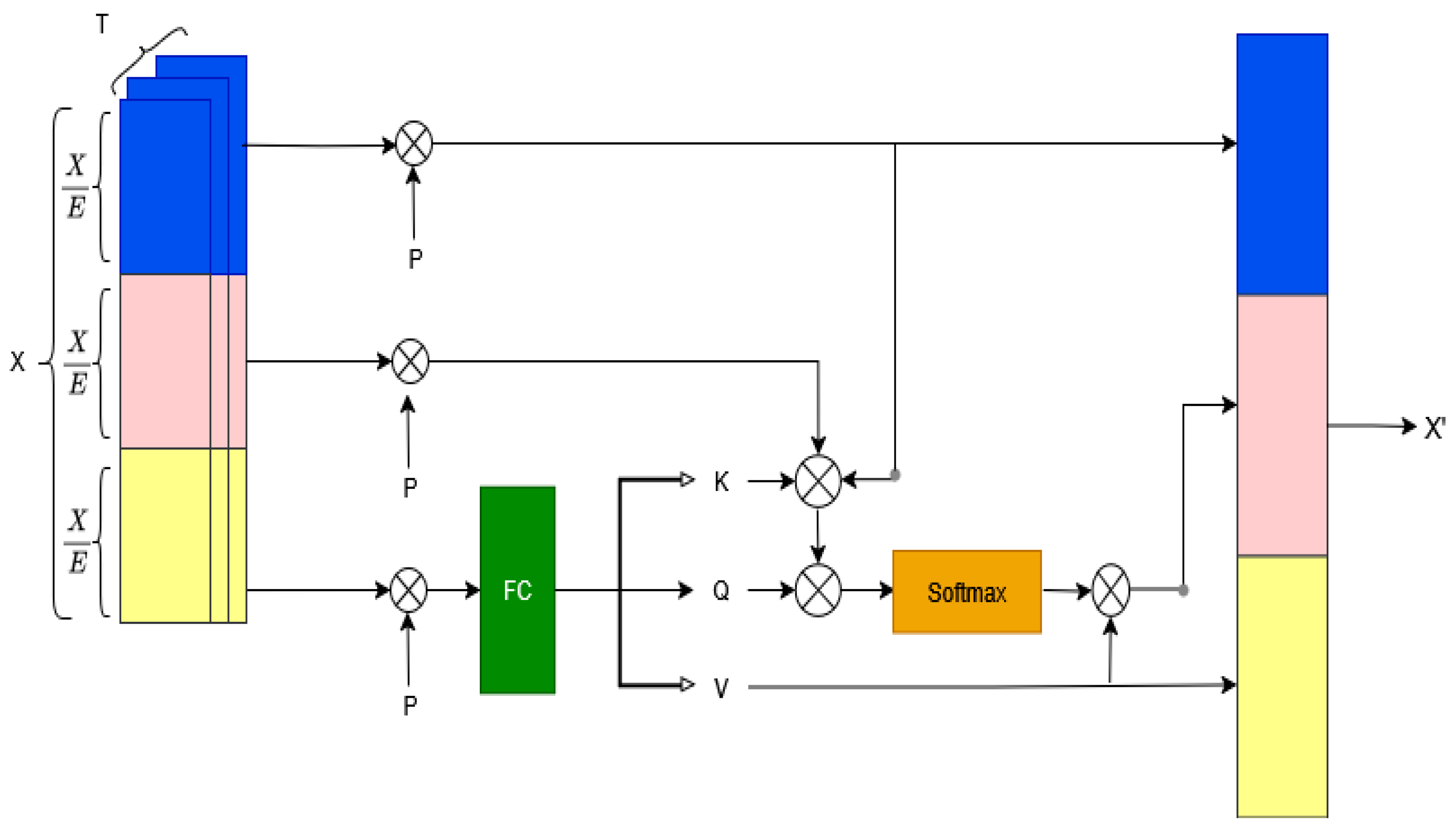
3.3. Multilevel Spatial-Temporal Graph Convolutional Network (MLAGCN)
Wind power forecasting presents complex challenges due to the spatial and temporal variability of wind conditions and the nonlinear relationships among turbine operations. To address these, we propose a unified framework that combines multiple specialized graph-based modules, each focusing on a different aspect of turbine behavior. Unlike prior spatio-temporal GCN frameworks that employ a single, static adjacency structure, our MLAGCN introduces a local-aware graph and a global-aware graph that enable simultaneous learning of turbine-specific dynamics and global meteorological dependencies, leading to improved generalization across heterogeneous wind conditions.
As shown in Figure 1, the architecture consists of four main components: the Local Aware Graph and the Global Aware Graph, inspired by [30], a Structure Aware Graph, and the Lightweight Temporal Transformer. The three graphs are combined element-wise to form the overall adaptive graph and then combined with the temporal transformer, with T denoting the number of time steps, C the feature dimension, and N the number of turbines. This graph integrates turbine-level local interactions, global meteorological dependencies, and latent structural relationships. The graph convolution operation is then performed as:
where represents the turbine features at time t, and are learnable parameters, and is the symmetrically normalized combined adjacency matrix. This formulation allows each turbine node to aggregate information from its dynamically weighted neighbors based on multi-level spatial correlations. The convolutional outputs Z are then propagated through temporal modules to capture temporal dynamics.
3.3.1. Local-Aware Graph
The Local Aware Graph is designed to extract detailed, turbine-specific correlations between input features such as wind speed, direction, and ambient temperature. These local relationships often reflect transient weather phenomena or mechanical responses that affect only a subset of turbines. Let the input be a 3D tensor , where T is the number of time steps (past hours), N is the number of turbines in the wind farm, and C is the number of feature channels. To model per-turbine feature importance, we first compute a local channel attention vector for each turbine independently.
For turbine , we extract its feature sequence over time , and apply global average pooling along the temporal axis, yielding a vector . This vector captures the average behavior of each feature for that specific turbine. Next, we project through a multilayer perceptron (MLP) followed by a sigmoid activation to obtain the local channel attention weights , computed as:
This attention highlights which features (channels) are most relevant for a specific turbine based on its own historical data. denotes average pooling over the time dimension.
Next, to incorporate turbine connectivity information, the local attention map is combined with the predefined structural graph, , which represents spatial adjacency based on turbine topology. The local graph-aware representation, as shown in Figure 5, is obtained by element-wise multiplication between and .
with . This operation integrates both the learned feature relevance and the physical interconnections among turbines, allowing the model to capture spatially localized dependencies while respecting the true network structure of the wind farm. The resulting local-graph-aware feature enhances the ability of the model to represent fine-scale spatial interactions influenced by immediate turbine neighborhoods.
3.3.2. Global-Aware Graph
The Global Aware Graph is designed to capture wide-scale, farm-level dependencies that are consistent across turbines and time. Such dependencies may arise from large-scale meteorological patterns, such as atmospheric fronts or diurnal wind shifts, which influence all turbines simultaneously. To extract this global context, we incorporate a global channel attention mechanism that emphasizes features most informative at the full farm level. For an input , we compute the average of all feature values across time. The resulting feature reflects the average magnitude of each feature across the entire wind farm and time horizon. To generate attention weights, we pass through a multilayer perceptron followed by a sigmoid activation and obtain a weight vector :
This vector identifies which features are globally important, such as temperature or wind speed, based on their average contribution across the spatiotemporal domain. To further incorporate physical turbine relationships, the predefined graph is introduced, producing the global-graph-aware graph representation as:
with . In Figure 5, we illustrate the design of the global-aware graph. This integration ensures that global dependencies are not only learned statistically but are also constrained by the underlying physical topology. Consequently, models consistent, wide-area spatial dependencies while maintaining coherence with turbine connectivity, effectively capturing large-scale weather patterns and their influence across the entire wind farm.
3.3.3. Structure-Aware Graph
While the local and global graph modules implicitly capture relationships using attention, the Structure Aware Graph explicitly learns the topology that governs information flow between turbines. This is critical in wind power forecasting, where the influence of one turbine on another may depend not just on geographical proximity but also on terrain effects, wake interactions, or coordinated operational patterns.
The Structure-Aware Graph is designed to learn latent relationships between turbines beyond geographic distance or statistical similarity. Each turbine is assigned a learnable embedding vector forming the embedding matrix . These embeddings encode turbine-specific characteristics and enable the model to infer hidden dependencies. A graph , is constructed by computing pairwise correlations between embeddings:
3.3.4. Temporal Module
Capturing the dynamic evolution of wind patterns over time is essential for accurate forecasting. The Temporal Self-Attention Module addresses this by applying attention across the temporal axis. First, we reduced the channle C dimension of the input tensor into H groups of size with H being the number of heads.
Self-attention is then applied on each group by projecting the input into query , key , and value matrices using learned weights , , , respectively. The attention output is computed as , where d is the dimensionality of the key vectors.
This mechanism enables the model to identify which past time steps are most relevant for predicting future output, while the inclusion of positional encodings ensures the model retains a sense of temporal order. The architecture of the temporal module is shown in Figure 2. The attention-enhanced outputs are then projected and added back to the original input sequence, producing a rich temporal representation that supports both long-term forecasting and short-term fluctuation tracking.
4. Experimental Setting
4.1. Dataset Processing
To maximize the utility of the SDWPF dataset, several feature engineering techniques are implemented. Initially, relevant features for model training are selected, and irrelevant or redundant features are removed based on correlation coefficient scores [2]. From the attributes listed in Table 1, five features are chosen: , , , , and . A new feature, , is constructed as the difference between at time step and at time step . Prior to training, Z-score normalization is applied to standardize the dataset inputs. During model training, the historical time series of each wind turbine is combined with data from different periods of the same wind turbine to enrich the data samples and reduce overfitting.
4.2. Evaluation Metrics
Wind power forecasting involves predicting the time series of wind power output at a wind farm. Due to the presence of outliers in the SDWPF dataset, prediction results are evaluated for each wind turbine individually. The prediction scores for all turbines are then aggregated to obtain the final model score. In this WPF work, the objective is to predict a future wind power supply time series of length 288. The evaluation metric is the average of the Root Mean Square Error (RMSE) and Mean Absolute Error (MAE). At time step , the evaluation score for wind turbine i is defined as follows:
where is the active power of the wind turbine i and is the active power predicted by the wind turbine i in the time step . At time step , the final score is the sum of the evaluation score on all the 134 wind turbines.
Outlier data are addressed using specific procedures. Reactive and active power values less than zero are set to zero. When wind turbines stop generating electricity due to external factors, such as equipment modifications or scheduled power supply adjustments to prevent grid overload, the actual generated active power is considered unknown and excluded from analysis. In this work, the target variable is classified as unknown under two conditions: At time step , if and , the actual active power is unknown; At time step , if any of Pab1, Pab2, or Pab3 exceeds 89°, the actual active power is unknown. Any abnormal value in a data column is excluded from the model evaluation. Two rules define abnormal values. At time step , if or , the actual active power Patv is abnormal, and at time step , if or , the actual active power Patv is abnormal.
4.3. Training Loss
The Huber loss [31] is selected as the training loss function for both models due to its reduced sensitivity to outliers compared to the squared error loss. The Huber loss is defined as follows:
In this formulation, denotes the threshold parameter that controls the sensitivity of the squared error. The variable represents the predicted active power of all wind turbines, while X denotes the ground-truth active power of all wind turbines. All predicted and ground-truth values have been processed according to the outlier handling rules described in Section 4.2.
4.4. Implementation Details
All experiments were conducted on Ubuntu 22.04 using an NVIDIA RTX A6000 GPU. The implementation was based on PyTorch 2.0 with CUDA 12.1 support. Following the settings adopted in prior studies on the SDWPF dataset, the model was trained to predict a future wind power sequence of length 288 using a historical sequence of 144 time steps. Training was performed using the Adam optimizer () with an initial learning rate of 0.001, regulated by a cosine annealing scheduler with warm restarts. The model parameters were initialized using Xavier uniform initialization, and dropout (0.2) was applied to mitigate overfitting. Early stopping with a patience of 10 epochs was used to prevent unnecessary training once convergence was achieved. No pretrained weights were used, and all parameters were learned from scratch to ensure fair comparison with previous works.
5. Discussion of Results
5.1. Comparison with the State of the Art
Table 2 summarizes the forecasting performance across nine competing models. Our proposed framework achieves an MAE of 38.83, an RMSE of 48.05, and a final evaluation score of 43.44, which surpasses several strong baseline methods, including the FDSTT (44.91) paper [32] that won the Baidu KDD Cup 2022 Challenge, the Fused Model (49.80) [33], and ARMA (50.52) [34]. Although the RMSE is marginally higher than a few baselines, MLAGCN consistently maintains a lower overall score, reflecting a balanced trade-off between accuracy and robustness. The performance of MLAGCN highlights the effectiveness of the adaptive multi-level attention mechanisms integrated into the spatial graph construction and the temporal learning modules. The gains can be attributed to MLAGCN’s ability to dynamically model both local and global spatial relationships, as well as its Transformer-based temporal attention mechanism that captures long-range dependencies.
While MLAGCN does not yield the absolute minimum MAE or RMSE, its overall score of 43.44 reflects improved forecasting stability and generalization, particularly in turbulent or fluctuating wind conditions.
These results validate the core hypothesis of this work that coupling adaptive graph learning with temporal attention leads to more reliable and accurate wind power forecasting across diverse turbine configurations and temporal horizons.
5.2. Ablation Study
To evaluate the effectiveness of each core component in our proposed MLAGCN framework, we conduct an ablation study by incrementally removing each module: Local-Aware Graph, Global-Aware Graph, Structure-Aware Graph, and the Temporal Transformer Module. All experiments are performed under the same settings as described in Section 4.4 using the SDWPF dataset. Results are shown in Table 3.
The ablation results clearly highlight the importance of each architectural component in achieving high-accuracy wind power forecasting. Notably, removing the Temporal Transformer Module leads to the largest decline in performance, increasing the overall score by more than 3.16 points. This underscores the pivotal role of temporal self-attention in capturing long-range dependencies and the sequential patterns inherent in wind dynamics, capabilities that traditional recurrent or convolutional modules often struggle to capture. The ability of the transformer to adaptively focus on relevant historical time steps proves crucial for accurate multi-step predictions.
Among the spatial modules, the Structure-Aware Graph contributes most significantly. Eliminating it results in a notable increase in forecasting error, demonstrating that learning a dynamic topology based on turbine embeddings is essential for modeling latent turbine-turbine interactions, especially in scenarios with complex wake effects or heterogeneous terrain. The Global-Aware Graph also proves vital, as its absence reduces the ability of the model to incorporate farm-wide meteorological trends, which are often correlated across geographically distant turbines. Finally, the Local-Aware Graph enhances performance by refining per-turbine feature importance, though its effect is somewhat more modest. Together, these results validate our modular design, in which each graph component captures a distinct spatial dependency, and the transformer module unifies these spatial cues over time.
6. Conclusions
In this study, we present MLAGCN, a novel graph convolutional network specifically designed for wind power forecasting, which addresses the dynamic and intricate spatial-temporal dependencies inherent in wind farm operations. MLAGCN features a multi-layered graph structure, integrating three complementary spatial graphs: the Global-Aware graph, which captures farm-wide contextual interactions; the Local-Aware graph, which focuses on immediate turbine neighborhoods; and the Structure-Aware graph, which encodes physical and operational connectivity among turbines. This layered design enables the model to learn both localized and holistic interaction patterns within the wind farm flexibly. Complementing the spatial module, we incorporate the Lightweight Temporal Transformer (LWTT), a transformer-based temporal module adept at modeling long-range sequential dependencies and capturing subtle temporal patterns in power output and meteorological conditions. By combining these advanced spatial and temporal mechanisms, the proposed architecture offers a comprehensive framework for accurate and robust wind power forecasting.
Extensive experiments were conducted on the widely used SDWPF real-world dataset to rigorously evaluate the effectiveness and robustness of MLAGCN. The results indicate that MLAGCN consistently outperforms established baseline models, delivering improvements in forecasting accuracy, stability, and generalization across multiple standard error metrics, including mean absolute error (MAE), root mean square error (RMSE), and normalized mean absolute error (NMAE). Ablation studies provide further insight into the model architecture, revealing that each spatial and temporal module makes a distinct and indispensable contribution to the overall performance. Adaptive spatial learning and temporal attention mechanisms are critical for capturing the nuanced dependencies present in wind farm data. These findings underscore the practical value and adaptability of MLAGCN for real-world wind power forecasting applications. Future work will focus on enhancing the model’s scalability for deployment in large-scale wind farms and integrating diverse external meteorological datasets to further strengthen multi-source learning and predictive capabilities.
Author Contributions
Conceptualization, O.E.D.; Methodology, O.E.D. and K.C.A; Software, K.C.A; Validation, O.E.D., K.C.A and D.K.; Formal analysis, O.E.D. and K.C.A.; Investigation, O.E.D. and K.C.A.; Resources, K.C.A.; Data curation, O.E.D. and K.C.A.; Writing—original draft preparation, O.E.D. and K.C.A.; Writing—review and editing, O.E.D. and D.K.; Visualization, O.E.D. and K.C.A.; Supervision, D.K.; Project administration, D.K.; Funding acquisition, D.K. All authors have read and greed to the published version of the manuscript.
Funding
This research was funded by the National Research Foundation of Korea (NRF) grant funded by the Korean government (MSIT) (RS-2024-00359150) and Basic Science Research Program through the National Research Foundation of Korea (NRF) funded by the Ministry of Education (RS-2019-NR040071).
Data Availability Statement
The original data presented in the study are openly available in the Baidu KDD Cup 2022 challenge repository at https://aistudio.baidu.com/competition/detail/152/0/introduction, with reference number [7].
Conflicts of Interest
The authors declare no conflicts of interest.
Abbreviations
The following abbreviations are used in this manuscript:
| MLAGCN | Multilevel Adaptive Graph Convolution Network |
| LWTT | Light Weight Temporal Transformer |
| MAE | Mean Absolute Error |
| RMSE | Root Mean Square Error |
| WPF | Wind Power Forecast |
| SDWPF | Spatial Dynamic Wind Power Forecasting |
| SCADA | Supervisory Control and Data Acquisition |
| MLP | Multilayer Perceptron |
| LAG | Local Aware Graph |
| GAG | Global Aware Graph |
References
- Nielsen, T.S.; Joensen, A.; Madsen, H.; Landberg, L.; Giebel, G. A new reference for wind power forecasting. Wind Energy: An International Journal for Progress and Applications in Wind Power Conversion Technology 1998, 1, 29–34.
- Wu, Z.; Luo, G.; Yang, Z.; Guo, Y.; Li, K.; Xue, Y. A comprehensive review on deep learning approaches in wind forecasting applications. CAAI Transactions on Intelligence Technology 2022, 7, 129–143. [CrossRef]
- Sideratos, G.; Hatziargyriou, N.D. An advanced statistical method for wind power forecasting. IEEE Transactions on power systems 2007, 22, 258–265. [CrossRef]
- Li, Z.; Ye, L.; Zhao, Y.; Pei, M.; Lu, P.; Li, Y.; Dai, B. A spatiotemporal directed graph convolution network for ultra-short-term wind power prediction. IEEE Transactions on Sustainable Energy 2022, 14, 39–54. [CrossRef]
- Song, Y.; Tang, D.; Yu, J.; Yu, Z.; Li, X. Short-term forecasting based on graph convolution networks and multiresolution convolution neural networks for wind power. IEEE Transactions on Industrial Informatics 2022, 19, 1691–1702. [CrossRef]
- Xu, H.; Zhang, Y.; Zhen, Z.; Xu, F.; Wang, F. Adaptive feature selection and GCN with optimal graph structure-based ultra-short-term wind farm cluster power forecasting method. IEEE Transactions on Industry Applications 2023, 60, 1804–1813. [CrossRef]
- Zhou, J.; Lu, X.; Xiao, Y.; Su, J.; Lyu, J.; Ma, Y.; Dou, D. Sdwpf: A dataset for spatial dynamic wind power forecasting challenge at kdd cup 2022. arXiv preprint arXiv:2208.04360 2022.
- Liu, G.; Zhang, Y.; Zhang, P.; Gu, J. Spatiotemporal graph contrastive learning for wind power forecasting. IEEE Transactions on Sustainable Energy 2025. [CrossRef]
- Li, J.; Armandpour, M. Deep Spatio-Temporal Wind Power Forecasting. In Proceedings of the ICASSP 2022 - 2022 IEEE International Conference on Acoustics, Speech and Signal Processing (ICASSP), 2022, pp. 4138–4142. https://doi.org/10.1109/ICASSP43922.2022.9747383. [CrossRef]
- Cui, Y.; Wang, P.; Meirink, J.F.; Ntantis, N.; Wijnands, J.S. Solar radiation nowcasting based on geostationary satellite images and deep learning models. Solar Energy 2024, 282, 112866. [CrossRef]
- Bansal, A.S.; Bansal, T.; Irwin, D. A moment in the sun: Solar nowcasting from multispectral satellite data using self-supervised learning. In Proceedings of the Proceedings of the thirteenth ACM international conference on future energy systems, 2022, pp. 251–262.
- Garnot, V.S.F.; Landrieu, L. Lightweight temporal self-attention for classifying satellite images time series. In Proceedings of the International Workshop on Advanced Analytics and Learning on Temporal Data. Springer, 2020, pp. 171–181.
- Brown, B.G.; Katz, R.W.; Murphy, A.H. Time series models to simulate and forecast wind speed and wind power. Journal of Applied Meteorology and Climatology 1984, 23, 1184–1195.
- Firat, U.; Engin, S.N.; Saraclar, M.; Ertuzun, A.B. Wind speed forecasting based on second order blind identification and autoregressive model. In Proceedings of the 2010 Ninth International Conference on Machine Learning and Applications. IEEE, 2010, pp. 686–691.
- Mohandes, M.A.; Halawani, T.O.; Rehman, S.; Hussain, A.A. Support vector machines for wind speed prediction. Renewable energy 2004, 29, 939–947. [CrossRef]
- Alexiadis, M.; Dokopoulos, P.; Sahsamanoglou, H.; Manousaridis, I. Short-term forecasting of wind speed and related electrical power. Solar Energy 1998, 63, 61–68. [CrossRef]
- Ahmadi, A.; Nabipour, M.; Mohammadi-Ivatloo, B.; Amani, A.M.; Rho, S.; Piran, M.J. Long-term wind power forecasting using tree-based learning algorithms. IEEE Access 2020, 8, 151511–151522. [CrossRef]
- Wang, H.z.; Li, G.q.; Wang, G.b.; Peng, J.c.; Jiang, H.; Liu, Y.t. Deep learning based ensemble approach for probabilistic wind power forecasting. Applied energy 2017, 188, 56–70. [CrossRef]
- Song, J.; Wang, J.; Lu, H. A novel combined model based on advanced optimization algorithm for short-term wind speed forecasting. Applied energy 2018, 215, 643–658. [CrossRef]
- Yu, R.; Gao, J.; Yu, M.; Lu, W.; Xu, T.; Zhao, M.; Zhang, J.; Zhang, R.; Zhang, Z. LSTM-EFG for wind power forecasting based on sequential correlation features. Future Generation Computer Systems 2019, 93, 33–42. [CrossRef]
- Zhou, H.; Zhang, S.; Peng, J.; Zhang, S.; Li, J.; Xiong, H.; Zhang, W. Informer: Beyond efficient transformer for long sequence time-series forecasting. In Proceedings of the Proceedings of the AAAI conference on artificial intelligence, 2021, Vol. 35, pp. 11106–11115. [CrossRef]
- Wu, H.; Xu, J.; Wang, J.; Long, M. Autoformer: Decomposition transformers with auto-correlation for long-term series forecasting. Advances in neural information processing systems 2021, 34, 22419–22430.
- Zhou, T.; Ma, Z.; Wen, Q.; Wang, X.; Sun, L.; Jin, R. Fedformer: Frequency enhanced decomposed transformer for long-term series forecasting. In Proceedings of the International conference on machine learning. PMLR, 2022, pp. 27268–27286.
- Zhao, Y.; Liao, H.; Pan, S.; Zhao, Y. Interpretable multi-graph convolution network integrating spatio-temporal attention and dynamic combination for wind power forecasting. Expert Systems with Applications 2024, 255, 124766.
- Qiu, H.; Shi, K.; Wang, R.; Zhang, L.; Liu, X.; Cheng, X. A novel temporal–spatial graph neural network for wind power forecasting considering blockage effects. Renewable Energy 2024, 227, 120499. [CrossRef]
- Jiang, J.; Han, C.; Wang, J. BUAA_BIGSCity: spatial-temporal graph neural network for wind power forecasting in Baidu KDD CUP 2022. arXiv preprint arXiv:2302.11159 2023.
- Liang, X.; Gu, Q.; Qiao, S.; Lv, Z.; Song, X. Team zhangshijin WPFormer: A Spatio-Temporal Graph Transformer with Auto-Correlation for Wind Power Prediction.
- Zhou, J.; Lu, X.; Xiao, Y.; Tang, J.; Su, J.; Li, Y.; Liu, J.; Lyu, J.; Ma, Y.; Dou, D. SDWPF: a dataset for spatial dynamic wind power forecasting over a large turbine array. Scientific Data 2024, 11, 649. [CrossRef]
- Evans, J.D. Straightforward statistics for the behavioral sciences.; Thomson Brooks/Cole Publishing Co, 1996.
- Song, C.H.; Han, H.J.; Avrithis, Y. All the attention you need: Global-local, spatial-channel attention for image retrieval. In Proceedings of the Proceedings of the IEEE/CVF winter conference on applications of computer vision, 2022, pp. 2754–2763.
- Huber, P.J. Robust estimation of a location parameter. In Breakthroughs in statistics: Methodology and distribution; Springer, 1992; pp. 492–518. [CrossRef]
- Li, L.; Sun, Q.; Geng, D.; Jian, C.; Wu, D.; Pu, S. Complementary fusion of deep spatio-temporal network and tree model for wind power forecasting (team: Hik) 2022.
- Kalander, M.; Rao, Z.; Zhang, C. Wind Power Forecasting with Deep Learning: Team didadida_hualahuala. In Proceedings of the Proceedings of Baidu KDD Cup 2022 - Wind Power Forecast (KDD ’22), New York, NY, USA, 2022; pp. 1–6. KDD Cup team paper.
- Ling-ling, L.; Li, J.H.; He, P.J.; Wang, C.S. The use of wavelet theory and ARMA model in wind speed prediction. In Proceedings of the 2011 1st International Conference on Electric Power Equipment-Switching Technology. IEEE, 2011, pp. 395–398.
- Ke, G.; Meng, Q.; Finley, T.; Wang, T.; Chen, W.; Ma, W.; Ye, Q.; Liu, T.Y. Lightgbm: A highly efficient gradient boosting decision tree. Advances in neural information processing systems 2017, 30.
Figure 3.
Scatterplot at wind turbine number 70.
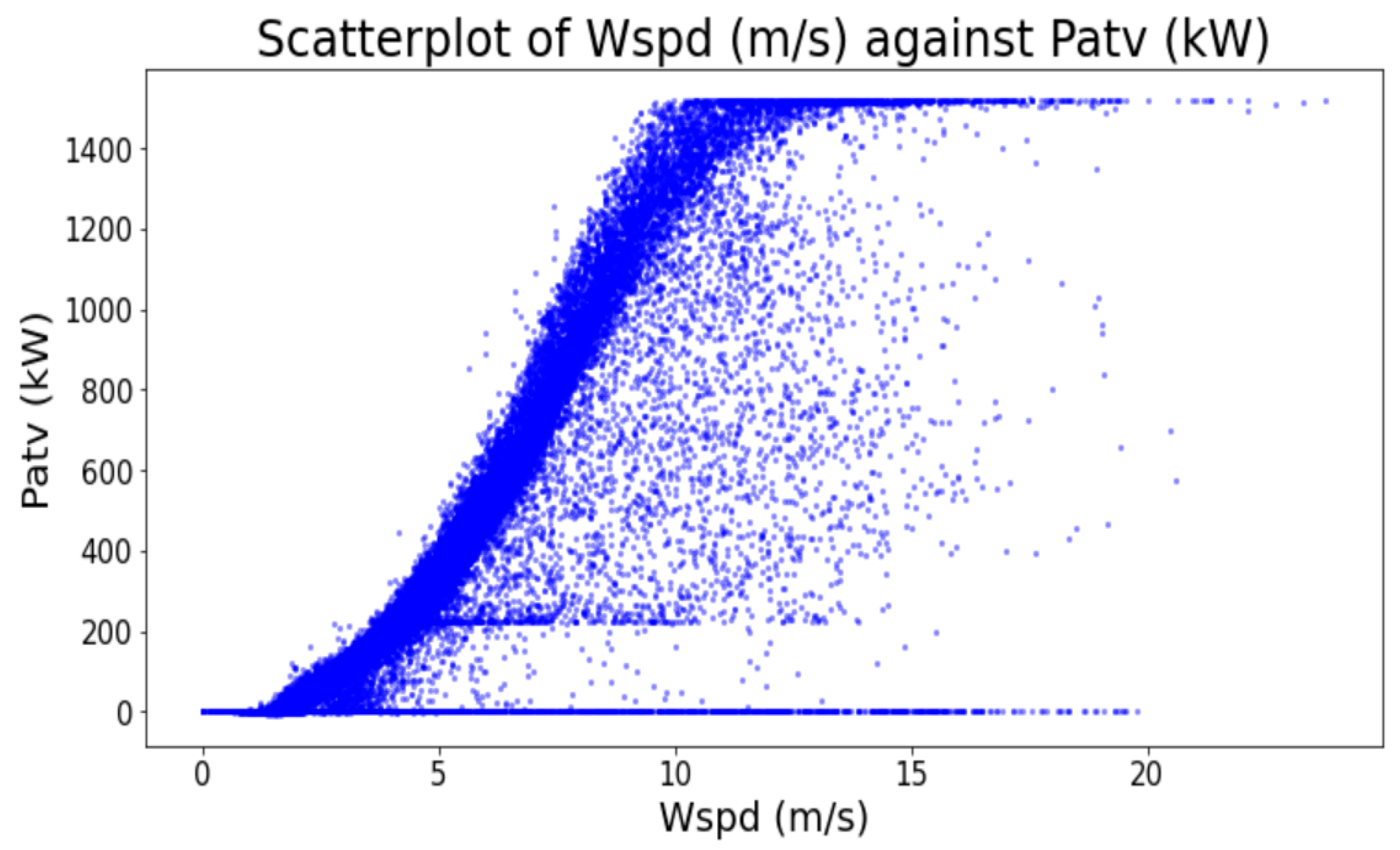
Figure 4.
Correlation matrix of features.
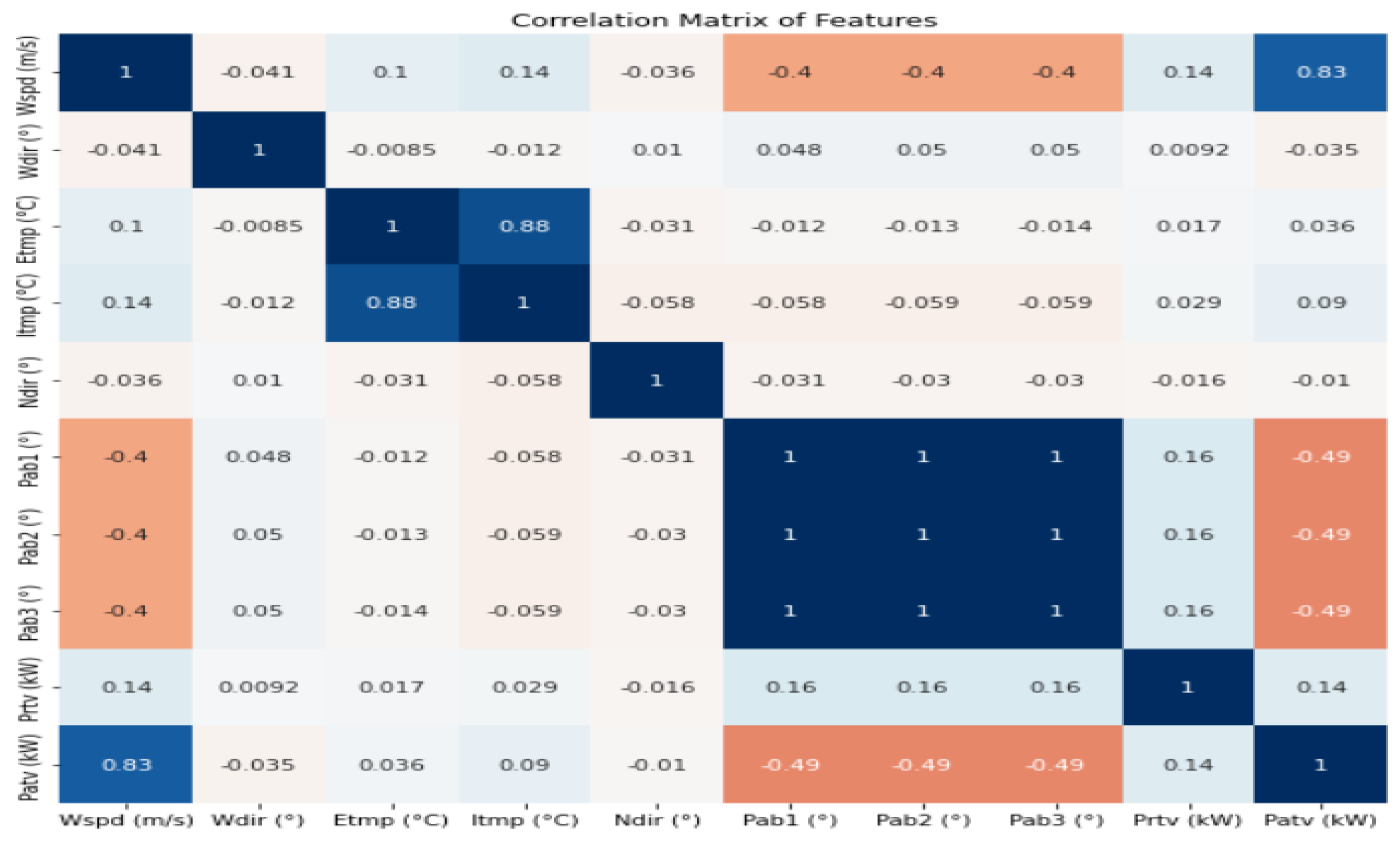
Figure 5.
Description of the Local-Aware Graph and Global-Aware Graph.
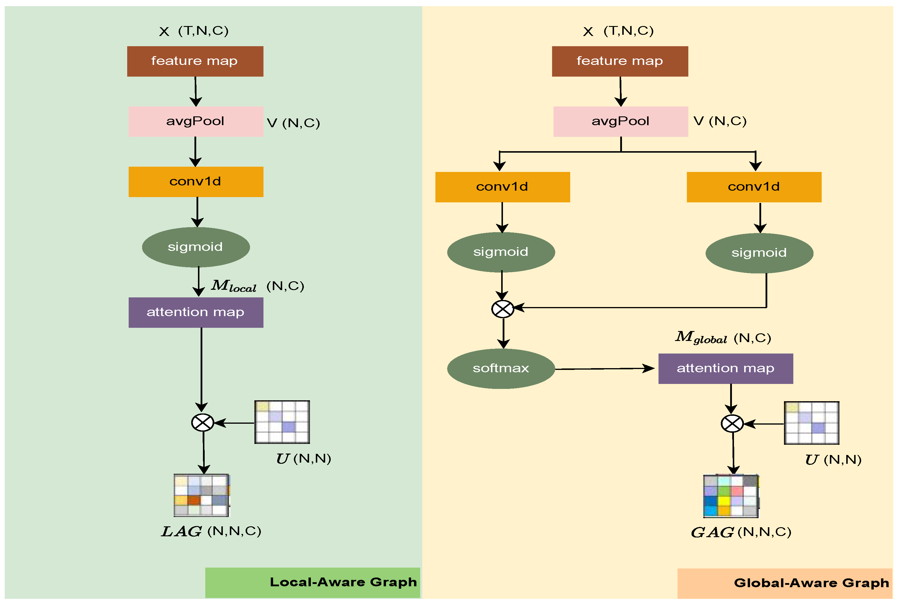

Table 1.
Column names and their specifications on the SDWPF dataset.
| Column | Column Name | Specification |
|---|---|---|
| 1 | TurbID | Wind turbine ID |
| 2 | Day | Day of the record |
| 3 | Tmstamp | Created time of the record |
| 4 | Wspd (m/s) | Wind speed recorded by the anemometer |
| 5 | Wdir (°) | Wind direction and turbine nacelle position angle |
| 6 | Etmp (°C) | Temperature of the surrounding environment |
| 7 | Itmp (°C) | Temperature inside the turbine nacelle |
| 8 | Ndir (°) | Nacelle direction, i.e. the yaw angle of the nacelle |
| 9 | Pab1 (°) | Pitch angle of blade 1 |
| 10 | Pab2 (°) | Pitch angle of blade 2 |
| 11 | Pab3 (°) | Pitch angle of blade 3 |
| 12 | Prtv (kW) | Reactive power |
| 13 | Patv (kW) | active power (target variable) |
Table 2.
The performance of different models.
| Model | MAE | RMSE | Score |
|---|---|---|---|
| ARMA [34] | 61.56 | 50.62 | 56.09 |
| GRU [6] | 55.13 | 45.77 | 50.45 |
| GNN [5] | 55.39 | 47.15 | 51.27 |
| LightGBM [35] | 53.05 | 44.89 | 48.97 |
| MDLinear (Single Model) [33] | 56.74 | 48.32 | 52.53 |
| MDLinear [33] | 53.40 | 45.53 | 49.46 |
| XTGN [31] | 54.54 | 46.50 | 50.52 |
| Fused Model [33] | 53.74 | 45.86 | 49.80 |
| FDSTT [32] | NA | NA | 44.91 |
Table 3.
Ablation study of different modules of MLAGCN.
| Model | MAE | RMSE | Score |
|---|---|---|---|
| Full MLAGCN (All Modules) | 38.83 | 48.06 | 43.45 |
| w/o Temporal Transformer | 41.92 | 51.28 | 46.60 |
| w/o Structure-Aware Graph | 40.51 | 49.63 | 45.07 |
| w/o Global-Aware Graph | 40.89 | 50.42 | 45.66 |
| w/o Local-Aware Graph | 40.26 | 50.01 | 45.14 |
Disclaimer/Publisher’s Note: The statements, opinions and data contained in all publications are solely those of the individual author(s) and contributor(s) and not of MDPI and/or the editor(s). MDPI and/or the editor(s) disclaim responsibility for any injury to people or property resulting from any ideas, methods, instructions or products referred to in the content. |
© 2025 by the authors. Licensee MDPI, Basel, Switzerland. This article is an open access article distributed under the terms and conditions of the Creative Commons Attribution (CC BY) license (http://creativecommons.org/licenses/by/4.0/).
Copyright: This open access article is published under a Creative Commons CC BY 4.0 license, which permit the free download, distribution, and reuse, provided that the author and preprint are cited in any reuse.


