
Submitted:
05 December 2025
Posted:
08 December 2025
You are already at the latest version
Abstract
This study presents a comprehensive nighttime contrail characterization combining Raman lidar, ADS-B flight data, and ECMWF ERA5 reanalysis over southern France. Observations of different case studies of contrail formation and development throughout their lifetimes provide valuable insights into the contrail’s morphological, microphysical, and optical properties, persistence, and dispersion.
We present a multi‑source methodology to detect and characterize nighttime aircraft contrails over the Observatory of Haute-Provence (OHP) in France. Determination of contrail’s signatures was performed by applying sensitivity analyses by spatiotemporal thresholding and clustering for contrail detection. Optimizing the thresholds permits improving contrail detection and reducing unnecessary noises.
Here, the optimal combination of these thresholds that better reduces false positives and negatives was SR = 2.1, time = 7.2 min, and altitude = 0.3 km. Subsequently merging the resulting spots yields persistent contrail signatures at altitudes of 8.7–10.3 km with thicknesses of 0.1–1.1 km, widths of 2–28 km, and optical depths of 0.05–0.40. Contrail optical depth correlates significantly with geometrical thickness and width and highlights the interplay between contrail morphology and ambient thermodynamic conditions. Our methodology demonstrates the value of combining lidar and flight data for contrail characterization, using lidar measurements, flight data, and meteorological information.
Keywords:
Contrail nighttime characterization
; Lidar
; ADS-B
; ECMWF ERA5 Reanalysis
1. Introduction
Climate change nowadays is a hot topic among the scientific community. Aviation contrails are considered a potential significant contributor to radiative forcing and consequently, to climate change, especially given the anticipated sharp rise in global air traffic [1]. Aviation contributes to non-CO2 climatic impacts through emissions of nitrogen oxide (NOX), water vapor, sulfate, and soot particles [2]. Persistent contrails and the contrail cirrus, together with sulfate aerosols, represent a major non-CO₂ component of aviation’s climate impact [3]. It is estimated, that their contribution on net warming is twice of that of its CO2 emissions, and the contribution of only contrail and contrail cirrus is about 1.5 times of that of aviation’s CO2 emissions. Their combined effective radiative forcing (ERF) is estimated to be as 67 mW m⁻² (5–95% CI), corresponding to roughly two-thirds of aviation’s net ERF in 2018 (101 [55–145] mW m⁻²) [2]. For the time being the Sixth Assessment Report (AR6), the global mean effective radiative forcing (mW.m–2) from combined contrails and contrail-induced cirrus +40 [+10 to +70] [4]. Recent studies attribute more than one-third of aircraft-related ERF to contrails alone, and current best estimates indicate that contrails and the aircraft-induced cirrus clouds they form account for about half of the anthropogenic ERF from aviation for the period 1940–2018. Given this significant contribution, systematic contrail observations and analysis of their formation, persistence and radiative properties are essential to reduce uncertainty in aviation-related climate forcing.
The fact that aircraft contrails exhibit optical properties similar to those of cirrus clouds and form in the same altitude range, makes it challenging to distinguish between them [5]. Contrails of any optical depth (COD) and their environmental conditions have been investigated by lidar systems in several studies [6,7,8,9,10,11,12]. Lidars, because they can provide accurate vertical profiles, are the most promising tool for contrail observation and investigation. On the other side, only the aged contrails with significative COD are observable by satellite imagery, such as the Spinning Enhanced Visible and InfraRed Imager (SEVIRI) onboard the Meteosat Second Generation (MSG) satellite, Advanced Very High Resolution Radiometer (AVHRR) [12] onboard the Meteorological Operational (MetOp), Terra and Aqua Moderate-resolution Imaging Spectroradiometer (MODIS) [13], Geostationary Operational Environmental Satellite (GOES) [14], etc. However, satellite observation is hampered by contrail’s low optical depth, small width, which is lower than the satellite spatial resolution. The combination of several of these tools enables the detection, and quantification of contrail properties, as well as the investigation of their life time, as illustrated in a recent one-day case study by [15].
Several studies [16,17] classify contrails into three types; young, mature, and old based on the morphology in terms of contrail width, shape (linearity), and edge sharpness (Table 1). The World Meteorological Organization has classified persistent contrails as the sole artificial cirrus clouds [18]. Persistent contrails gradually spread out, transitioning into contrail cirrus that can merge with existing natural or other contrail cirrus. Their evolution can also be influenced by long-range transport of air masses. These contrail cirrus can also be advected over long distances by large-scale atmospheric circulation, altering their spatial extent and optical properties, that control also their persistence [19]. Contrail cirrus have optical depth two to three times higher than the contrails itself [20]. These contrails can develop up to hundreds of kilometers long, nevertheless still shorter than natural cirrus that extend up to thousands of kilometers, but can also be used as proxy for climate impact studies.
These studies have identified contrails on the limited vertical extent with substantial backscattering, as compared with surrounding cirrus. Altitude of contrails is concentrated mainly at 7-14 km [18,21,22,23]. Noise is considered as any isolated feature in the lidar profiles with a width less than 1 km and thickness less than 60 m.
While satellite imagery contrail studies are more common [24,25,26], nighttime detection remains not fully explored. A more challenging point is that the persistence of the contrails is obtained mostly during the morning hours where the relative and wind updraft are maximal, and less during our measuring time [27]. This study cross over this gap using synergistic lidar measurements and collocated information provided by flight data provider.
The goal of this study is to comprehensively investigate microphysical and morphological evolution of individual contrails combining collocated nighttime Rayleigh–Mie–Raman lidar observations, flight tracking, and ERA5 dataset. This objective was reached through developing contrail detection algorithm, retrieve contrail geometry and compute their optical properties, and thermodynamic contextualization regarding their persistence criteria.
We present a night-time contrail characterization over OHP that jointly optimizes lidar-based detection thresholds with spatio-temporal grouping, and cross-checks events against flight-track passages and ERA5 dynamics and thermodynamics. Beyond the lidar measurements, we (i) optimize detection/discrimination thresholds through conducting sensitivity analyses to select optimal thresholds of scattering-ratio (SR), time, and altitude that maximize COD and contrail duration which reduces false negatives/positives; (ii) derive their geometry (altitude, thickness, width, axis orientation) and optical properties (COD, SRmax) for each contrail signature; and (iii) contextualize these properties with ERA5 meteorology data (T, RHice, RHliq, PV, etc.) to diagnose their persistence conditions. This multi-source, threshold-optimized framework provides a reproducible pathway for contrail monitoring at night when passive imagery is unavailable, complementing recent ERA5-based climatologies and satellite radiative analyses.
The paper is organized as follows: Section 2 describes thoroughly the methodology; starting from the procedure of contrail retrievals, describing instrumentation used, such as lidar, flight provider and ECMWF-ERA5 reanalysis dataset. Additionally, in this section, the contrail detection thresholds are explained too. Section 3 presents the detailed results and discussions for all the case studies of the contrails. The conclusions of this study are presented in the Section 4.
2. Materials and Methods
2.1. Contrail Retrievals
To detect contrails and investigate their geometrical properties, we used the collocated lidar and Automatic Dependent Surveillance-Broadcast (ADS-B) data as previously described [28]. This is done through temporal synchronization and spatial matching of lidar measurements and with flight passage times [29,30,31].
The contrail’s vertical extend is estimated from the altitude-resolved lidar backscatter profiles. Contrail’s width is derived from wind speed provided by ECMWF ERA5 data, and their duration is estimated from the persistence time of the contrail signature in the lidar signal. This methodology has been also applied previously [15].
Backscattering lidar profiles analyzed in this study have been provided by the Rayleigh-Mie-Raman lidar, situated at the Observatory of Haute Provence in France (43.9° N, 5.7° E, and 673 meters altitude), which conducts only night-time measurements, usually operating for about 6 hours per session [7,8,32]. This lidar uses a frequency-doubled Nd-YAG laser which emits a light pulse of approximately 10 nanoseconds at 532 nm, with a repetition rate of 30 Hz and an average pulse energy of 300 mJ. The telescope field-of-view is 1 mrad [33]. The cirrus detection system consists of a primary lens, an interference filter, The vertical resolution of lidar measurements is 15 m, while the temporal resolution is 60 s, which enables the instrument to detect fresh contrails and contrail cirrus too [34].
The lidar measurements have been carried out during the period between 2021 and 2023. The lidar scattering ratio profiles have been used to identify the signatures which suggest the presence of the contrails [34]. Based on the information provided by the altitude-resolved profiles, the contrail optical and geometrical properties, such as the contrail mean altitude, geometrical thickness (CGT), contrail optical depth (COD), and their orientations are determined.
The process of retrieving contrail optical depth using a lidar involves making certain assumptions. COD was obtained from SR profiles by the following expression given by [35]. So, the contrail optical depth at a certain altitude z is given by integrating the total volume scattering coefficient β(z).
Further on, the total volume scattering coefficient β(z) is given as the product of the total scattering cross section per molecule σ(z) and the molecular number density nair(z). The contrail optical depth is determined using the previous assumptions, as follow:
where the Rayleigh-Scattering Cross Section σ=5.4x10⁻³¹ m2 [35,36,37,38].
The lidar scattering ratio was obtained from the Mie and Rayleigh scattering coefficients, and it is defined as the ratio of the particulate backscattering (excluding background aerosol contribution) to the total backscattering:
In particle-free conditions, SR is equal to unity.
Multiple scattering correction η of the contrails are calculated based on the simplified Eq. 6, [39,40,41,42]:
where, COD is the contrail’s optical depth.
Nevertheless, η does not only depend on the COD but also on ice crystal effective radius and laser beam field of view and penetration depth [43,44,45]. In a more specific formulation, also because of their ice content, contrails can be considered as thin cirrus clouds, even of their sharp difference in backscattering signal with the surroundings. Many studies have used different values of η on assessing the cirrus cloud optical depth [46,47,48,49,50,51,52,53,54,55]. A value of 0.9 for subvisual cirrus clouds, 0.8 for moderate thick cirrus and 0.6 to 0.7 for opaque cirrus was used by [47]. Other study, [48], suggested the following values for different temperature ranges; 0.54 (at -60 oC), 0.65 (at -40 oC) and 0.76 (at -20 oC). Multiple scattering factor have been analyze by [49], inferred from CALIPSO of cirrus clouds, suggested η of 0.50 (at 240 K) and 0.80 (at 200 K). Similarly, studying cirrus clouds by CALIPSO products, [50] suggested η of 0.60, meanwhile. Lower values, 0.60 (thicker than 1 km) and 0.70 (thinner than 1 km) were used by [51,52]. Higher η of 0.75 have used [53]. Regarding to the previous contrail studies, [6,54,55] have used a η of 0.70. This study has used the same value of multiple scattering correction, 0.70, a value that can also be applied to contrails.
A variety of the lidar ratios (LR) are used in analyzing cirrus clouds. Hence, [8,35] used a LR of 18 sr, [56,57] used higher LR (25 sr), while even higher value of LR (31 sr) was used by [52]. Fewer papers analyze contrails using specific lidar ratios. Hence, [58] who observed contrails over Boulder, Colorado and used a variable SR of 13–40 sr. 20 sr was used by [59], an intermediate LR of 25 sr was used by [6], and even a lower LR of 16 sr to investigate both cirrus and contrails was used by [60]. The lidar ratio in this paper is chosen LR=25 sr, as in many similar studies [6,34,61].
2.2. Contrail detection thresholds and their properties
In total, seven cases have been analyzed, during a tree night-time observation. Determination of the geometrical contours of the contrails is done though the optimization of effective thresholds.
In addition, ERA5 (the 5th generation of atmospheric reanalysis of the global climate and provided by the Copernicus Climate Change Service (C3S) at European Centre for Medium-Range Weather Forecasts (ECMWF) is used, to assess the environmental conditions around contrails [62,63]. Meteorological atmospheric, and ERA5’s information about wind speed and direction, help to obtain contrail’s geometrical width during their temporal lifespan. Additionally, mid-contrail temperature (T), relative humidity over liquid and ice (RHliq and RHice), and potential vorticity (PV) have been analyzed [5]. It is assumed that during the period when the contrail appears above the lidar, meteorological parameters remain constant.
We have performed sensitivity analyses to optimize contrail detection based on the lidar scattering ratio (SR) threshold and to optimize their discrimination using temporal and altitude distance thresholds. Sensitivity analysis optimize detection/discrimination via maximization of COD and contrail duration while preserving the observed event count. Robustness of the procedure is tested under the variations: SR ± (5–10%), LR (25–31 sr) and η (0.6–0.8). These events are cross-checked against flight overpasses and ISSR persistence criteria (T < Tcrit; RHice > 100%). This sensitivity analysis enables us to reduce false positive and false negative in the detection of separate contrails, also to avoid their misinterpretation.
For each profile, we identify cases where SR and minimum thickness Δz exceed their thresholds to suppress single-bin noises. Profiles are then aggregated in space (t, z) using proximity thresholds (time and altitude) to form continuous contrails signatures. The aggregation of these single nearby spots envelopes the space occupied by each contrail.
After determining the contrail’s signatures, their morphology and optical properties have been taken into analyses. For each signature we derive mean altitude, thickness, width (from the lidar timespan multiplied with the ERA5 cross-track wind), duration, density (SRmax), COD, the major-axis orientation (slope in t–z space). This procedure can be applied for automatic contrail detection.
A schematic representation of this procedure of contrail signatures detection, though varying SR, altitude and time thresholds is presented by Figure 1. Aggregation of the spikes gives more insights on the identification of properties of the contrail events.
3. Results and Discussions
3.1. Contrail geometrical features, case studies
The investigation of the contrail’s morphological features and optical properties over OHP, is focused on several case studies, regarding young contrails under cloud-free and cloudy conditions. Among these properties, mid-contrail’s altitude, vertical extent and duration are the principal parameters taken into consideration.
3.1.1. Contrail cases during 13.01.2023
A representing special case of the multi - contrails formed under clear-sky conditions is identified during 13.01.2023, (Figure 2). Flight data provider suggest that several flight over OHP coincide with the lidar spikes observations. So, during the lidar measuring period from 17:25 to 21:25, four major spikes were observed in the altitude profile of SR, having potentially contrail signature origins. Combining information from both sources, it results that these four lidar spikes co-occur with the flights of 2, 1, 4 and 2 planes over OHP at the corresponding intervals.
There is not a significative difference in the aircraft speeds, during all cases. Also, flight direction is almost the same, around 140o. The flight altitudes range from the upper-troposphere to the tropopause (7.9-10.3 km). The projected distance from the lidar is similar for all flights (~2-3 km), except one during 3rd case, which overpass almost exactly over the OHP site (~500 m). Aircraft designs, are different during these cases, dominated by Airbus model A319 and A320. Almost all aircrafts are of 2 turbofan engines (models Airbus and Boeing), only during case III, a 3-turbofan engine aircraft (Dassault Falcon FA7X) flighted over the site. Kerosene was utilized as fuel in every of these aircrafts [64].
The first two neighbor signatures represent two contrail events, each of them having the life span of 17:47-17:53 and 17:55-18:04, respectively.
To simplify the identification of the signal spikes in the lidar SR profiles, an aggregation procedure was applied to the nearby signatures. This procedure enables a better identification of individual contrails. To determine the optimal thresholds of the lidar scattering ratio for contrail detection, as well as the temporal and spatial separation criteria for distinguishing single contrails, a sensitivity analysis was conducted. This approach helps to minimize false positive/negative detections.
To process with the aggregation, the lidar scattering ratio threshold was chosen as in the interval 1.5-5.0, by step 0.5. Temporal difference thresholds were chosen in the range 5-30 min (increasing monotonically in 1 min steps, while the spatial difference thresholds ranged from 0.1 to 2.5 km (increasing monotonically in 200 m steps). Figure 3 shows the results of the sensitivity analysis.
Figure 3 indicates that lower SR thresholds result in higher mean COD values. This is because SR values lower than their threshold are not taken into account in the COD calculation, underestimating it. In addition, low SR threshold count also the weaker contrails, increasing the detection sensitivity. On the other side, high SR threshold decrease the sensitivity but improve the detection significance, taking into account only undisputed contrail cases. In our case there are prioritized combinations with high COD and high contrail counts, balancing so sensitivity and significance. Shorter time thresholds provide more precise aggregation but might fragment some long-lasting contrails (false positive), while longer time thresholds detect more continuous contrails but risk grouping no-contrail events (false negative). Smaller space thresholds despite of the altitude precision but might split contrails into multiple groups (false positive), while larger space thresholds might aggregate different contrails (false negative).
To obtain the optimal threshold values, for each of the parameters, large and stable values of the mean COD and contrail duration, across the variation of the temporal and spatial thresholds are required. However, the specific constrains, such as spatial and temporal differences between flights passages over the site during each special case, should be taken into account to obtain the optimal threshold values. After performing the sensitivity analysis, in order to obtain the maximal value of contrail optical depth and duration, maintaining the required number of groups, the optimal values of these threshold result to be one of the combinations (Table 2).

Table 2.
Flight characteristics during the four potential contrail cases; contrail cases, time of occurrence (UTC+2), flight altitude (km), speed (km/h) and direction (grades), horizontal distance (km) from the lidar site, aircraft type, engines and fuel used.
Table 2.
Flight characteristics during the four potential contrail cases; contrail cases, time of occurrence (UTC+2), flight altitude (km), speed (km/h) and direction (grades), horizontal distance (km) from the lidar site, aircraft type, engines and fuel used.
| Cases | Time | Altitude | Speed | Direction | Dist. | Type | Engines | Fuel |
|---|---|---|---|---|---|---|---|---|
| I | 17:17 | 7.9 | 832 | 138 | 2.8 | Airbus A320 | 2 turbofan | kerosene |
| 17:22 | 8.6 | 948 | 140 | 2.0 | Airbus A319 | 2 turbofan | kerosene | |
| II | 17:43 | 10.3 | 1007 | 141 | 2.6 | Dassault Falcon FA7X | 3 turbofan | kerosene |
| III | 18:24 | 10.2 | 893 | 137 | 0.5 | Boeing B738 | 2 turbofan | kerosene |
| 18:29 | 10.3 | 941 | 141 | 2.4 | Airbus A320 | 2 turbofan | kerosene | |
| 18:46 | 8.6 | 943 | 140 | 3.1 | Airbus A320 | 2 turbofan | kerosene | |
| 18:48 | 9.8 | 963 | 142 | 3.4 | Airbus A320 | 2 turbofan | kerosene | |
| IV | 19:03 | 8.9 | 832 | 142 | 3.0 | Airbus A20N | 2 turbofan | kerosene |
| 19:26 | 7.9 | 859 | 140 | 2.9 | Airbus A319 | 2 turbofan | kerosene |
Table 2.
Summarized results of the sensitivity analysis regarding to the thresholds of backscatter ratio, time and altitude, to detect and discriminate the four contrail events. This procedure is based on the optimization of the contrail’s properties; COD, duration, and their number.
Table 2.
Summarized results of the sensitivity analysis regarding to the thresholds of backscatter ratio, time and altitude, to detect and discriminate the four contrail events. This procedure is based on the optimization of the contrail’s properties; COD, duration, and their number.
| Time (min) | SR | Altitude (km) |
Time (min) |
COD | Duration (min) |
Count |
|---|---|---|---|---|---|---|
| Range of thresholds | 0.1-2.5 | 5-30 | 5.8-13.8 | 4 | 0.10-0.40 | 1.5-5.0 |
| Optimal combinations | 0.3-1.0 | 5-15 | 7.2 | 4 | 0.40 | 2.0-2.5 |
| Selection | 0.3 | 7.2 | 7.2 | 4 | 0.40 | 2.1 |
Best combinations of the thresholds are those that maximize the mean COD and the duration of the contrails. These combinations better configure the geometrical parameters of the four principal peaks that corresponding to the contrails.
Among the several threshold combinations, we have chosen the best one, which maximize contrail COD and duration. This combination uses a contrail detection threshold SR=2.1 and contrail spatial-temporal discrimination thresholds of 0.3 km and 10-15 min. Because both temporal thresholds yield same results, the 7.2 min temporal threshold is maintained due to the flight traffic frequency above the site (Figure 4). This case represents, clear-sky condition. However, in cirrus environments higher scatter ratio should be used [65].
The timespan of the contrail detection by lidar, is converted into contrail’s width, using wind direction and speed provided by ERA5. The wind directions have been projected perpendicularly with the contrail’s principal axis to provide their geometrical width. The timespan is different from the contrail lifetime, which is its life starting from its emission up to the total dispersion. Nevertheless, the lidar backscattering profiles don’t provide total information of the contrail’s lifetime. To give more insight over the contrail properties, the Table 3 provides their mean values of these properties for each group.
Table 3 provides insight into the geometrical and optical properties of the four contrail cases on 13.01.2023. The 3rd case is by far the thinnest, but at the same time the widest among the others. Previous works of [66,67], regarding the relations between contrail vertical extend and their age, suggest that all these cases represent contrails aged between 15 min and 30 min old. The amplified width of the 3rd case is due to the overlapping of two simultaneous very thin contrails over the site. Only the 4th case is characterized by a positive slope of the contrail principal axis, whereas the other cases present a negative slope. This suggest that case maybe characterized by uplift wind profiles. The relative humidity with respect to ice is significantly higher than 100% in all four cases. Hence, the environment during the four cases at the cruise altitudes result to be supersaturated with respect to ice. So, there are perfect conditions for contrails persistence. However, to be formed, contrails need to have temperature below the critical temperature and relative humidity with respect to water higher than its respective critical value. Critical temperatures for all cases range from -43.2 to -42.1 oC, whereas the actual temperature during these cases is well below these limits; ranging from -61.2 to -56.1 oC. To this end, this condition is clearly fulfilled. Also, RHliq ranging 70-90%, overcome the critical values for all of cases. Based on the categorization presented in the Table 3, the circumstances of the four cases, can be considered as persistent contrails (RHice > 100%). Contrail’s optical depth fits well to those reported by [68,69] except the case 3, where a very optically thin contrail was observed.
3.1.2. Additional suspicious cases
Furthermore, other three potential contrail’s signatures are examined in this section. A second young contrail case, this time, under cloudy conditions, was observed on 03.03.2022. The indicated signature on the SR lidar profiles in Figure 5, shows the contrail spike. Additionally, two suspicious signatures under cloud-free conditions (25.11.2022), are shown by Figure 6.
Similar to the Table 3, also the Table 4 present the ensemble of the contrail parameters during the young contrail event under cloudy conditions (case 5), and during two other suspicious cases under cloud-free conditions (cases 6 and 7).
Given the Schmidt-Appleman and ISSR criteria, case 5 represents a persistent contrail, while cases 6 and 7 represent cases that don’t fulfill the contrail formation and persistence criteria. Being under supersaturation conditions (RHice > 100%), it guaranties the persistence of the contrail of case 5. It is plausible that their respective spots during the cases 6 and 7 are result of non-contrail products. This assumption is also supported by the signature width, which in the case 5 suits reasonably with the contrail’s width, while in the cases 6 and 7 their width is largely wider than for usual contrails (> 10 km). Additionally, there are identified many cases on which no contrail spots in the lidar SR profiles, while aircrafts overfly the OHP site. During these cases, obviously the contrail formation criteria weren’t fulfilled, and represent only NoC cases. No significative differences among the cases 5-7 regarding to the orientations of the signature axes, which were almost fully horizontal. Also, their altitude, temperature, geometrical thickness, ice water content, were quite comparable among these cases.
The small slopes (close to zero) for the case 5, indicates that the contrail signature is nearly parallel to the isentropic surfaces, which is typical in the upper troposphere, where vertical wind shear is generally not significant, and atmospheric stability allows their persistence. The persistent contrail, case 5, is obtained at lower altitudes compared to that reported by [6], having comparable COD with those of [26,68,69]. Its geometrical features, width and thickness, are inside the rage suggested by [4], but significantly smaller than those reported by [6].
The threshold used to determine the contrail boundary affects estimates of their thickness and width. Taken into consideration all the five contrail cases, their mean contrail width was comparable to that of old contrail reported by [6], while mean thickness is slightly higher than those of young contrails found from the same source.
The background cloud environment substantially alters contrail evolution. Thus, significant differences are observed between the four persistent contrails formed under clear-sky conditions on 13.01.2023 (cases #1–4) and the contrail observed beneath an overlying cirrus deck on 03.05.2022 (case #5). Case #5 is formed at 8.7 km in a higher supersaturated conditions and beneath cirrus located ~3 km above, resulting in enhanced optical signatures (SRmax≈13 and COD≈0.33), but being thinner (0.3 km) and narrower (1.4 km). This alteration reflects radiative coupling with the cirrus layer, which reduces longwave cooling at the contrail top and stabilizes the environment, sustaining ice-crystal growth [18,26]. Thus, while all cases satisfy formation and persistence criteria, the cirrus-overlying structure leads to denser contrails compared with those evolving in clean upper-tropospheric conditions.
The correlation-based visualization provided by the network correlation diagram (Figure 7) gives insights about the interrelationships among several contrail geometrical, optical and thermodynamic properties. Thermodynamic parameters such as temperature (T), relative humidity (RHliq and RHice), and PV tend to be more correlated. These parameters potentially share the same atmospheric conditions, like atmospheric stability and moisture availability, that govern these variables.
Also, optical parameters, such as optical depth (COD) and density (SRmax) show moderate correlations with geometrical properties (e.g., thickness and width). This suggests that microphysical characteristics that impact the optical parameters are influenced by the contrail geometry.
Higher RHice values indicate favorable ISS conditions, that stimulate the ice crystal formation and growth within contrails. Consequently, IWC result to be positively correlated to RHice. In addition, IWC which indicate the concentration of ice crystals has positive feedback on COD.
Correlation coefficients of the mean altitude suggest that high-altitude contrails tend to be thinner and wider, so more horizontally dispersed. Both, SRmax, contrail thickness and their optical depth result strongly correlated. COD is directly related to both contrail thickness and lidar spikes. However, contrails with higher particle density in their centre result to be also thicker.
Contrail’s vertical and temporal extensions are generally expected to be positively correlated, implying that thicker contrails persist for longer durations. Interestingly, in this study, these parameters are found to be negatively correlated. The duration represents the horizontal contrail dimension, corresponding to the projection of its width along the wind direction. Hence, the inverse relationship between vertical and horizontal contrail dimensions suggests the conservation of contrail volume, whereas changes in shape may be primarily due to atmospheric dynamics. The more horizontally dispersed a contrail is, the less geometrically and optically thick it tends to be. Previous studies have shown that dispersion, influenced by wind shear, affects both the geometric and optical properties of contrails, as well as their coverage [70,71].
Interesting fact is that the contrail orientation results slightly positively correlated with their altitude and density. It may be respect to the windy patterns at upper-tropospheric regions, which enforce contrail alignment [72].
However, these correlations do not provide the full picture of the situation. This is because contrail parameters depend strongly on the contrail’s density and on its current stage of life. Also, the orientation, represented here as the slope of the main contrail axis during its detection period, is influenced not only by the thermodynamical state of the atmosphere, but also by variability in aircraft flight altitudes, which prevents a clear dependence of orientation on the meteorological factors. Finally, due to the limited number of cases considered, the relationships obtained should be interpreted with caution.
Nevertheless, it is worth highlighting that these assessments are based on a limited sample size. Larger datasets would provide a more comprehensive understanding.
4. Conclusions
This paper presents a study of contrail properties based on lidar measurements, flight data and the ECMWF ERA5 reanalysis dataset. Among the seven events analyzed, five were confirmed as persistent contrails, fulfilling both the formation and persistence criteria, while the other two cases don’t represent contrail cases.
The study demonstrates that a scattering ratio threshold of ~2.1 with temporal and spatial separations of ~7.2 min and ~0.3 km effectively identifies contrails and discriminates them from surrounding noises, such are cirrus clouds. All persistent contrails occurred within ice-super-saturated layers and at temperatures below -41 oC. Geometrical contrail properties such as thickness, width and orientation, are 0.58±0.40 km, 11.7±11.3 and quasi horizontal orientation.
The proposed detection and grouping procedure can be applied for automatic processing, enabling routine, automated identification and characterization of contrails from lidar data supplemented by flight tracks and ERA5.
Regarding the inter-relationships between optical and geometrical properties, contrail optical depth clearly increases with both vertical thickness and horizontal width, suggesting that optical properties can serve as proxies for geometrical dimensions. This reflects the influence of contrail microphysical characteristics on geometry. Meteorological variables (temperature, relative humidity and wind shear) are significantly correlated due to shared atmospheric conditions, emphasizing the importance of the meteorological conditions in contrail evolution. Also, due to the crystal growth, contrail optical depth results correlated with RHice and ice water content. Contrail orientation shows a slight positive correlation with altitude, due to upper-tropospheric wind patterns.
Another important result of this analysis is the difference between geometric properties of the contrails under clear sky conditions and those situated beneath cirrus clouds. Radiative effects of the present cirrus, alter the environmental conditions, particularly contrail dispersion, impacting so their persistency.
Having various implications for remote sensing and climate models, the multi-source approach shows that combining lidar backscatter with flight data provider information yields reliable contrail detection and further characterization. Such a data combination can be used to validate satellite retrievals and improve contrail parameterizations in climate models.
The sample is relatively small and limited to a single region. Future work should include more extensive observational data to different locations and atmospheric conditions, in synergy with satellite observations, and additional tools such are visible/thermal cameras. This will help to generalize the findings and reduce ambiguities related to the origin of the lidar signal signatures.
Author Contributions
Conceptualization, P.K. and F.M.; methodology, F.M. P.K.; software, F.M.; validation, F.M., P.K. and S.K.; formal analysis, F.M.; investigation, F.M.; resources, P.K.; data curation, F.M. and S.K.; writing—original draft preparation, F.M.; writing—review and editing, A.I, F.P., J-L.B., D.A., A.S., S.K. and P.K.; visualization, F.M. D.A.; supervision, P.K.; project administration, P.K.; funding acquisition, P.K. All authors have read and agreed to the published version of the manuscript.
Funding
This study also benefits from scientific support within the CONTRAILS and BeCoM projects, in which CNRS and UVSQ participates. This work is additionally supported by CNES through the EarthCARE contrail detection project, as part of the ground-based preparation activities using lidar and complementary atmospheric observations.
Data Availability Statement
The data supporting the findings of this study are available from the corresponding author upon reasonable request.
Acknowledgments
This study makes use of lidar observations from the Observatory of Haute-Provence (OHP). ERA5 reanalysis data were provided by the European Centre for Medium-Range Weather Forecasts (ECMWF) and generated from the Copernicus Climate Change Service (C3S).
Conflicts of Interest
The authors declare no conflicts of interest. The funders had no role in the design of the study; in the collection, analyses, or interpretation of data; in the writing of the manuscript; or in the decision to publish the results.
References
- Singh, D.K.; Sanyal, S.; Wuebbles, D.J. Understanding the role of contrails and contrail cirrus in climate change: a global perspective. Atmos. Chem. Phys. 2024, 24, 9219–9262. [Google Scholar] [CrossRef]
- Lee, D.; Fahey, D.; Skowron, A.; Allen, M.; Burkhardt, U.; Chen, Q.; Doherty, S.; Freeman, S.; Forster, P.; Fuglestvedt, J.; et al. The contribution of global aviation to anthropogenic climate forcing for 2000 to 2018. Atmospheric Environ. 2021, 244, 117834. [Google Scholar] [CrossRef] [PubMed]
- Teoh, R.; Engberg, Z.; Schumann, U.; Voigt, C.; Shapiro, M.; Rohs, S.; Stettler, M.E.J. Global aviation contrail climate effects from 2019 to 2021. Atmos. Chem. Phys. 2024, 24, 6071–6093. [Google Scholar] [CrossRef]
- Intergovernmental Panel on Climate Change. IPCC, Climate Change 2021: The Physical Science Basis. Contribution of Working Group I to the Sixth Assessment Report of the Intergovernmental Panel on Climate Change; Masson-Delmotte, V., Ed.; Cambridge University Press: Cambridge, UK, 2021; Available online: https://www.ipcc.ch/report/ar6/wg1/ (accessed on 30 November 2025).
- Bryukhanov, I.; Loktyushin, O.; Ni, E.; Samokhvalov, I.; Pustovalov, K.; Kuchinskaia, O. Comparison of the Contrail Drift Parameters Calculated Based on the Radiosonde Observation and ERA5 Reanalysis Data. Atmosphere 2024, 15, 1487. [Google Scholar] [CrossRef]
- Keckhut, P.; Hauchecorne, A.; Bekki, S.; Colette, A.; David, C.; Jumelet, J. Indications of thin cirrus clouds in the stratosphere at mid-latitudes. Atmos. Chem. Phys. 2005, 5, 3407–3414. [Google Scholar] [CrossRef]
- Keckhut, P.; Borchi, F.; Bekki, S.; Hauchecorne, A.; SiLaouina, M. Cirrus classification at mid-latitude from systematic lidar observations. J. Appl. Meteorol. Clim. 2006, 45, 249–258. [Google Scholar] [CrossRef]
- Keckhut, P.; Perrin, J.-M.; Thuillier, G.; Hoareau, C.; Porteneuve, J.; Montouxc, N. Subgrid-scale cirrus observed by lidar at mid-latitude: variability effects of the cloud optical depth. J. Appl. Remote Sens. 2013, 7, 073530. [Google Scholar] [CrossRef]
- Xu, M.; Meijer, V.; Barrett, S.R.H.; Eastham, S.D. Evaluation of the APCEMM intermediate-fidelity contrail model using LIDAR observations. In Proceedings of the American Geophysical Union (AGU) Fall Meeting, San Francisco, CA, USA, 11–15 December 2023. [Google Scholar]
- Alraddawi, D.; Keckhut, P.; Mandija, F.; Sarkissian, A.; Pietras, C.; Dupont, J.-C.; Farah, A.; Hauchecorne, A.; Porteneuve, J. Calibration of Upper Air Water Vapour Profiles Using the IPRAL Raman Lidar and ERA5 Model Results and Comparison to GRUAN Radiosonde Observations. Atmosphere 2025, 16, 351. [Google Scholar] [CrossRef]
- Dione, C.; Dupont, J.-C.; Caillault, K.; Gourgue, N.; Pietras, C.; Haeffelin, M. Estimation of optical and microphysical characteristics of contrails using Lidar at SIRTA observatory, Paris. In Proceedings of the EGU General Assembly 2025, Vienna, Austria, 14–19 April 2025. [Google Scholar] [CrossRef]
- Kalluri, S.; Cao, C.; Heidinger, A.; Ignatov, A.; Key, J.; Smith, T. The advanced very high resolution radiometer: Contributing to earth observations for over 40 years. Bull. Amer. Meteorol. Soc. 2021, 102, E351–E366. [Google Scholar] [CrossRef]
- Duda, D.P.; Bedka, S.T.; Minnis, P.; Spangenberg, D.; Khlopenkov, K.; Chee, T.; Smith, W.L., Jr. Northern Hemisphere contrail properties derived from Terra and Aqua MODIS data for 2006 and 2012. Atmos. Chem. Phys. 2019, 19, 5313–5330. [Google Scholar] [CrossRef]
- Kärcher, B.; Burkhardt, U.; Unterstrasser, S.; Minnis, P. Factors controlling contrail cirrus optical depth. Atmos. Chem. Phys. 2009, 9, 6229–6254. [Google Scholar] [CrossRef]
- Diarra, S.; Baray, J.-L.; Montoux, N.; et al. Combining LIDAR, all-sky camera, and ECMWF-ERA5 reanalysis to investigate contrail formation and evolution over Clermont-Ferrand, France on June 2, 2023. Atmospheric Research 2025, 213, 108500. [Google Scholar] [CrossRef]
- Rap, A.; Forster, P.M.; Jones, A.; Boucher, O.; Haywood, J.M.; Bellouin, N.; De Leon, R.R. Parameterization of contrails in the UK Met Office Climate Model. J. Geophys. Res.-Atmos 2010, 115, D10205. [Google Scholar] [CrossRef]
- Wolf, K.; Bellouin, N.; Boucher, O. Long-term upper-troposphere climatology of potential contrail occurrence over the Paris area derived from radiosonde observations. Atmos. Chem. Phys. 2023, 23, 287–309. [Google Scholar] [CrossRef]
- Kärcher, B. Formation and Radiative Forcing of Contrail Cirrus. Nat. Commun. 2018, 9, 1824. [Google Scholar] [CrossRef] [PubMed]
- Megill, L.; Grewe, V. Investigating the limiting aircraft-design-dependent and environmental factors of persistent contrail formation. Atmos. Chem. Phys. 2025, 25, 4131–4149. [Google Scholar] [CrossRef]
- Minnis, P.; Bedka, S.T.; Duda, D.P.; Bedka, K.M.; Chee, T.; Ayers, J.K.; Palikonda, R.; Spangenberg, D.A.; Khlopenkov, K.V.; Boeke, R. Linear contrail and contrail cirrus properties determined from satellite data. Geophys. Res. Lett. 2013, 40, 3220–3226. [Google Scholar] [CrossRef]
- Voigt, C.; Coauthors. ML-CIRRUS: The Airborne Experiment on Natural Cirrus and Contrail Cirrus with the High-Altitude Long-Range Research Aircraft HALO. Bull. Amer. Meteor. Soc. 2017, 98, 271–288. [Google Scholar] [CrossRef]
- Paoli, R.; Shariff, K. Contrail Modeling and Simulation. Ann. Rev. Fluid Mech. 2016, 48, 393–427. [Google Scholar] [CrossRef]
- Lamquin, N.; Stubenrauch, C.J.; Gierens, K.; Burkhardt, U.; Smit, H. A global climatology of upper-tropospheric ice supersaturation occurrence inferred from the Atmospheric Infrared Sounder calibrated by MOZAIC. Atmos. Chem. Phys. 2012, 12, 381–405. [Google Scholar] [CrossRef]
- Marjani, S.; Tesche, M.; Bräuer, P.; Sourdeval, O.; Quaas, J. Satellite observations of the impact of individual aircraft on ice crystal number in thin cirrus clouds. Geophys. Res. Lett. 2022, 49, e2021GL096173. [Google Scholar] [CrossRef]
- Jarry, G.; Very, P.; Heffar, A.; Torjman-Levavasseur, V. Deep semantic contrails segmentation of GOES-16 satellite images: A hyperparameter exploration. In Proceedings of the SESAR Innovation Days 2024, Brussels, Belgium, 3–6 December 2024. [Google Scholar]
- Wang, X.; Wolf, K.; Boucher, O.; Bellouin, N. Radiative effect of two contrail cirrus outbreaks over Western Europe estimated using geostationary satellite observations and radiative transfer calculations. Geophys. Res. Lett. 2024, 51, e2024GL108452. [Google Scholar] [CrossRef]
- Yu, J.; Zhou, X.; Li, L.; Gao, L.; Li, X.; Pan, W.; Ni, X.; Wang, Q.; Chen, F. High-resolution thermal infrared contrails images identification and classification method based on SDGSAT-1. Int. J. Appl. Earth Obs. Geoinf 2024, 131, 103980. [Google Scholar] [CrossRef]
- Peyrin, F.; Fréville, P.; Montoux, N.; Baray, J.-L. Original and Low-Cost ADS-B System to Fulfill Air Traffic Safety Obligations during High Power LIDAR Operation. Sensors 2023, 23, 2899. [Google Scholar] [CrossRef] [PubMed]
- Wolf, K.; Bellouin, N.; Boucher, O. Distribution and morphology of non-persistent contrail and persistent contrail formation areas in ERA5. Atmos. Chem. Phys. 2024, 24, 5009–5024. [Google Scholar] [CrossRef]
- Geraedts, S.; et al. A scalable system to measure contrail formation on a per-flight basis. Environ. Res. Commun. 2024, 6, 015008. [Google Scholar] [CrossRef]
- Hofer, S.; Gierens, K.; Rohs, S. How well can persistent contrails be predicted? An update. Atmos. Chem. Phys. 2024, 24, 7911–7925. [Google Scholar] [CrossRef]
- Sherlock, V.; Garnier, A.; Hauchecorne, A.; Keckhut, P. Implementation and validation of a Raman lidar measurement of middle and upper tropospheric water vapour. Appl. Opt. 1999, 38, 5838–5850. [Google Scholar] [CrossRef]
- Khaykin, S.; Godin-Beekmann, S.; Hauchecorne, A.; Pelon, J.; Ravetta, F.; Keckhut, P. Stratospheric smoke layer with unprecedentedly high backscatter observed by lidars above southern france. Geophys. Res. Lett. 2018, 45, 1639–1646. [Google Scholar] [CrossRef]
- Mandija, F.; Keckhut, P.; Alraddawi, D.; Khaykin, S.; Sarkissian, A. Climatology of Cirrus Clouds over Observatory of Haute-Provence (France) Using Multivariate Analyses on Lidar Profiles. Atmosphere 2024, 15, 1261. [Google Scholar] [CrossRef]
- Goldfarb, L.; Keckhut, P.; Chanin, M.L.; Hauchecorne, A. Cirrus climatological results from lidar measurements at OHP (44°N, 6°E). Geophys. Res. Lett. 2001, 28, 1687–1690. [Google Scholar] [CrossRef]
- Sneep, M.; Ubachs, W. Journal of Quantitative Spectroscopy & Radiative Transfer 2005, 92, 293–310.
- Bates, R.D. Rayleigh scattering by air. Planet Space Sci. 1984, 32, 785–790. [Google Scholar] [CrossRef]
- Bucholtz, A. Rayleigh-scattering calculations for the terrestrial atmosphere. Appl. Opt. 1995, 34, 2765–2773. [Google Scholar] [CrossRef]
- Platt, C. Lidar and radiometric observations of cirrus clouds. J. Atmos. Sci. 1973, 30, 1191–1204. [Google Scholar] [CrossRef]
- Sassen, K.; Cho, B.S. Subvisual-thin cirrus lidar dataset for satellite verification and climatological research. J. Appl. Meteorol. 1992, 31, 1275–1285. [Google Scholar] [CrossRef]
- Chen, W.N.; Chiang, C.W.; Nee, J.B. Lidar ratio and depolarization ratio for cirrus clouds. Appl. Opt. 2002, 41, 6470–6476. [Google Scholar] [CrossRef]
- Nakoudi, K.; Stachlewska, I.; Ritter, C. An extended lidar-based cirrus cloud retrieval scheme: first application over an Arctic site. Opt. Express 2021, 29, 8553–8580. [Google Scholar] [CrossRef]
- Wandinger, U.; Tesche, M.; Seifert, P.; Ansmann, A.; Müller, D.; Althausen, D. Size matters: Influence of multiple scattering on CALIPSO light-extinction profiling in desert dust. Geophys. Res. Lett. 2010, 37, L00E08. [Google Scholar] [CrossRef]
- Shcherbakov, V.; Szczap, F.; Alkasem, A.; Mioche, G.; Cornet, C. Empirical model of multiple-scattering effect on single-wavelength lidar data of aerosols and clouds. Atmos. Meas. Tech. 2022, 15, 1729–1754. [Google Scholar] [CrossRef]
- Shcherbakov, V.; Szczap, F.; Mioche, G.; Cornet, C. Multiple-scattering effects on single-wavelength lidar sounding of multi-layered clouds. Atmos. Meas. Tech. 2024, 17, 3011–3028. [Google Scholar] [CrossRef]
- Gil-Díaz, C.; Sicard, M.; Comerón, A.; dos Santos Oliveira, D.C.F.; Muñoz-Porcar, C.; Rodríguez-Gómez, A.; Lewis, J.R.; Welton, E.J.; Lolli, S. Geometrical and optical properties of cirrus clouds in Barcelona, Spain: analysis with the two-way transmittance method of 4 years of lidar measurements. Atmos. Meas. Tech. 2024, 17, 1197–1216. [Google Scholar] [CrossRef]
- Sassen, K.; Comstock, J. A midlatitude cirrus cloud climatology from the facility for atmospheric remote sensing. Part III: Radiative properties. J. Atmos. Sci. 2001, 58, 2113–2127. [Google Scholar] [CrossRef]
- Platt, C.M.R.; Dilley, A.C. Remote Sounding of High Clouds. IV: Observed Temperature Variations in Cirrus Optical Properties. J. Atmos. Sci. 1981, 38, 1069–1082. [Google Scholar] [CrossRef]
- Garnier, A.; Pelon, J.; Vaughan, M.A.; Winker, D.M.; Trepte, C.R.; Dubuisson, P. Lidar multiple scattering factors inferred from CALIPSO lidar and IIR retrievals of semi-transparent cirrus cloud optical depths over oceans. Atmos. Meas. Tech. 2015, 8, 2759–2774. [Google Scholar] [CrossRef]
- Young, S.A.; Vaughan, M.A.; Kuehn, R.E.; Winker, D.M. The Retrieval of Profiles of Particulate Extinction from Cloud–Aerosol Lidar and Infrared Pathfinder Satellite Observations (CALIPSO) Data: Uncertainty and Error Sensitivity Analyses. J. Atmos. Oceanic Technol. 2013, 30, 395–428. [Google Scholar] [CrossRef]
- Seifert, P.; Ansmann, A.; Müller, D.; Wandinger, U.; Althausen, D.; Heymsfeld, A.J.; Massie, S.T.; Schmitt, C. Cirrus optical properties observed with lidar, radiosonde, and satellite over the tropical Indian Ocean during the aerosol-polluted northeast and clean maritime southwest monsoon. J. Geophys. Res. 2007, 112, D17205. [Google Scholar] [CrossRef]
- Dionisi, D.; Keckhut, P.; Liberti, G.L.; Cardillo, F.; Congeduti, F. Midlatitude cirrus classification at Rome Tor Vergata through a multichannel Raman-Mie-Rayleigh lidar. Atmos. Chem. Phys. 2013, 13, 11853–11868. [Google Scholar] [CrossRef]
- Hoareau, C.; Keckhut, P.; Noel, V.; Chepfer, H.; Baray, J.-L. A decadal cirrus clouds climatology from ground-based and spaceborne lidars above the south of France (43.9° N–5.7° E). Atmos. Chem. Phys. 2013, 13, 6951–6963. [Google Scholar] [CrossRef]
- You, Y.; Kattawar, G.W.; Yang, P.; Hu, Y.X.; Baum, B.A. Sensitivity of depolarized lidar signals to cloud and aerosol particle properties. J. Quant. Spectrosc. Radiat. Transfer 2006, 100, 470–482. [Google Scholar] [CrossRef]
- Hostetler, C.A.; Liu, Z.; Reagan, J.A.; Vaughan, M.A.; Winker, D.M.; Osborn, M.T.; Hunt, W.H.; Powell, K.A.; Trepte, C.R. CALIPSO Algorithm Theoretical Basis Document; NASA: Washington, DC, USA, 2005. [Google Scholar]
- Nohra, R.; Parol, F.; Dubuisson, P. Comparison of Cirrus Cloud Characteristics as Estimated by A Micropulse Ground-Based Lidar and A Spaceborne Lidar CALIOP Datasets Over Lille, France (50.60 N, 3.14 E). EPJ Web Conf. 2016, 119, 16005. [Google Scholar] [CrossRef]
- Giannakaki, E.; Balis, D.S.; Amiridis, V.; Kazadzis, S. Optical and geometrical characteristics of cirrus clouds over a Southern European lidar station. Atmos. Chem. Phys. 2007, 7, 5519–5530. [Google Scholar] [CrossRef]
- Langford, A.O.; Portmann, R.W.; Daniel, J.S.; Miller, H.L.; Eubank, C.S.; Solomon, S.; Dutton, E.G. Retrieval of ice crystal effective diameters from ground-based near-infrared spectra of optically thin cirrus. J. Geophys. Res. 2005, 110, D22201. [Google Scholar] [CrossRef]
- Jones, H.M.; Haywood, J.; Marenco, F.; O'Sullivan, D.; Meyer, J.; Thorpe, R.; Gallagher, M.W.; Krämer, M.; Bower, K.N.; Rädel, G.; Rap, A.; Woolley, A.; Forster, P.; Coe, H. A methodology for in-situ and remote sensing of microphysical and radiative properties of contrails as they evolve into cirrus. Atmos. Chem. Phys. 2012, 12, 8157–8175. [Google Scholar] [CrossRef]
- Immler, F.; Treffeisen, R.; Engelbart, D.; Krüger, K.; Schrems, O. Cirrus, contrails, and ice supersaturated regions in high pressure systems at northern mid latitudes. Atmos. Chem. Phys. 2008, 8, 1689–1699. [Google Scholar] [CrossRef]
- Iwabuchi, H.; Yang, P.; Liou, K.N.; Minnis, P. Physical and optical properties of persistent contrails: Climatology and interpretation. J. Geophys. Res.-Atmos 2012, 117, D06215. [Google Scholar] [CrossRef]
- Hersbach, H.; Bell, B.; Berrisford, P.; Biavati, G.; Horányi, A.; Muñoz Sabater, J.; Nicolas, J.; Peubey, C.; Radu, R.; Rozum, I.; et al. ERA5 hourly data on pressure levels from 1979 to present. Copernicus Climate Change Service (C3S) Climate Data Store (CDS) Available online. 2018. [Google Scholar] [CrossRef]
- Hersbach, H.; Bell, B.; Berrisford, P.; Biavati, G.; Horányi, A.; Muñoz Sabater, J.; Nicolas, J.; Peubey, C.; Radu, R.; Rozum, I.; et al. ERA5 monthly averaged data on pressure levels from 1979 to present. Copernicus Climate Change Service (C3S) Climate Data Store (CDS) Available online. 2019. [Google Scholar] [CrossRef]
- Wasiuk, D.K.; Khan, M.A.H.; Shallcross, D.E.; Lowenberg, M.H. A Commercial Aircraft Fuel Burn and Emissions Inventory for 2005–2011. Atmosphere 2016, 7, 78. [Google Scholar] [CrossRef]
- Groß, S.; Jurkat-Witschas, T.; Li, Q.; Wirth, M.; Urbanek, B.; Krämer, M.; Weigel, R.; Voigt, C. Investigating an indirect aviation effect on mid-latitude cirrus clouds – linking lidar-derived optical properties to in situ measurements. Atmos. Chem. Phys. 2023, 23, 8369–8381. [Google Scholar] [CrossRef]
- Freudenthaler, V.; Homburg, F.; Jäger, H. Contrail observations by ground-based scanning lidar: Cross-sectional growth. Geophys. Res. Lett. 1995, 22, 3501–3504. [Google Scholar] [CrossRef]
- Poellot, M.R.; Arnott, W.P.; Hallett, J. In situ observations of contrail microphysics and implications for their radiative impact. J. Geophys. Res.-Atmos 1999, 104, 12077–12084. [Google Scholar] [CrossRef]
- Sassen, K. Contrail-cirrus and their potential for regional climate change. Bull. Amer. Meteor. Soc. 1997, 78, 1885–1903. [Google Scholar] [CrossRef]
- Atlas, D.; Wang, Z. Contrails of Small and Very Large Optical Depth. J. Atmos. Sci. 2010, 67, 3065–3073. [Google Scholar] [CrossRef]
- Rosenow, J.; Fricke, H. Individual Condensation Trails in Aircraft Trajectory Optimization. Sustainability 2019, 11, 6082. [Google Scholar] [CrossRef]
- Kumar, B.; Ranjan, R.; Yau, M.-K.; Bera, S.; Rao, S.A. Impact of high- and low-vorticity turbulence on cloud–environment mixing and cloud microphysics processes. Atmos. Chem. Phys. 2021, 21, 12317–12329. [Google Scholar] [CrossRef]
Figure 1.
Contrail signatures aggregated into four groups by varying the optimal combinations of their detections and discriminations thresholds. Linear trend-lines indicate their principal axes in the space time – altitude. The contrail properties shown in the legend are the maximal value of the backscattering ratio in the middle of the contrails and the spatial-temporal surface covered by them.
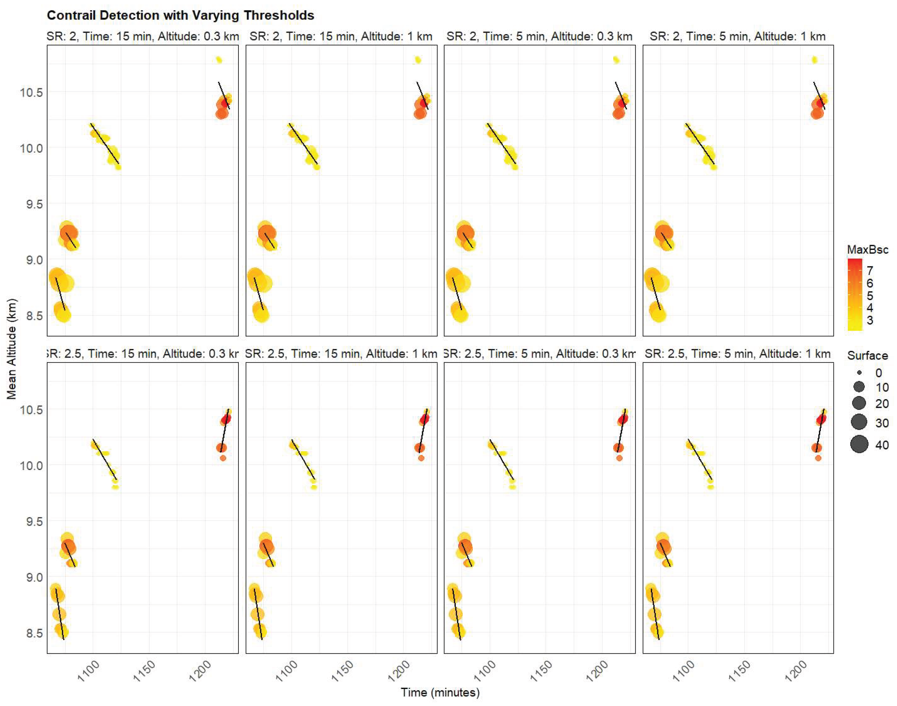
Figure 2.
Altitude-resolved profiles of the lidar scattering ratio (SR) during 13.01.2023 over OHP. Four contrail events have been identified. Yellow arrows indicate these contrail signatures.
Figure 2.
Altitude-resolved profiles of the lidar scattering ratio (SR) during 13.01.2023 over OHP. Four contrail events have been identified. Yellow arrows indicate these contrail signatures.
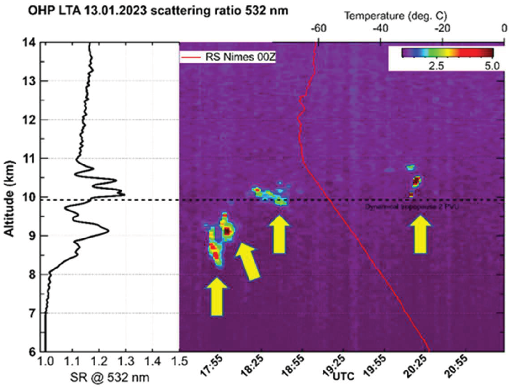
Figure 3.
Sensitivity analysis for the a) optimal determination of contrail detection based on the threshold of lidar scattering ratio, and b) optimal contrail discrimination based on the time- and altitude distance signature’ thresholds.
Figure 3.
Sensitivity analysis for the a) optimal determination of contrail detection based on the threshold of lidar scattering ratio, and b) optimal contrail discrimination based on the time- and altitude distance signature’ thresholds.
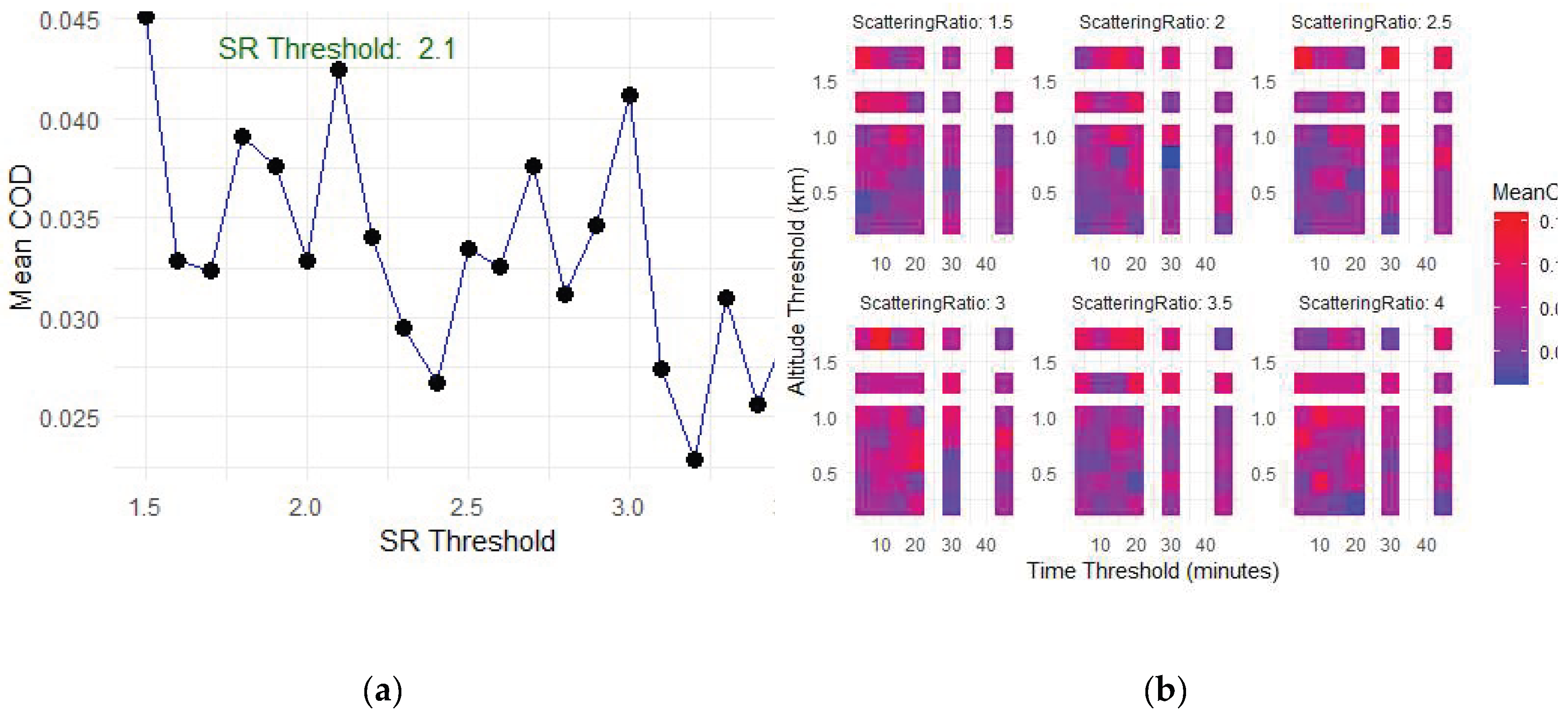
Figure 4.
indicates that lower SR thresholds result in higher mean COD values. This is because SR values lower than their threshold are not taken into account in the COD calculation, underestimating it. In addition, low SR threshold count also the weaker contrails, increasing the detection sensitivity. On the other side, high SR threshold decrease the sensitivity but improve the detection significance, taking into account.
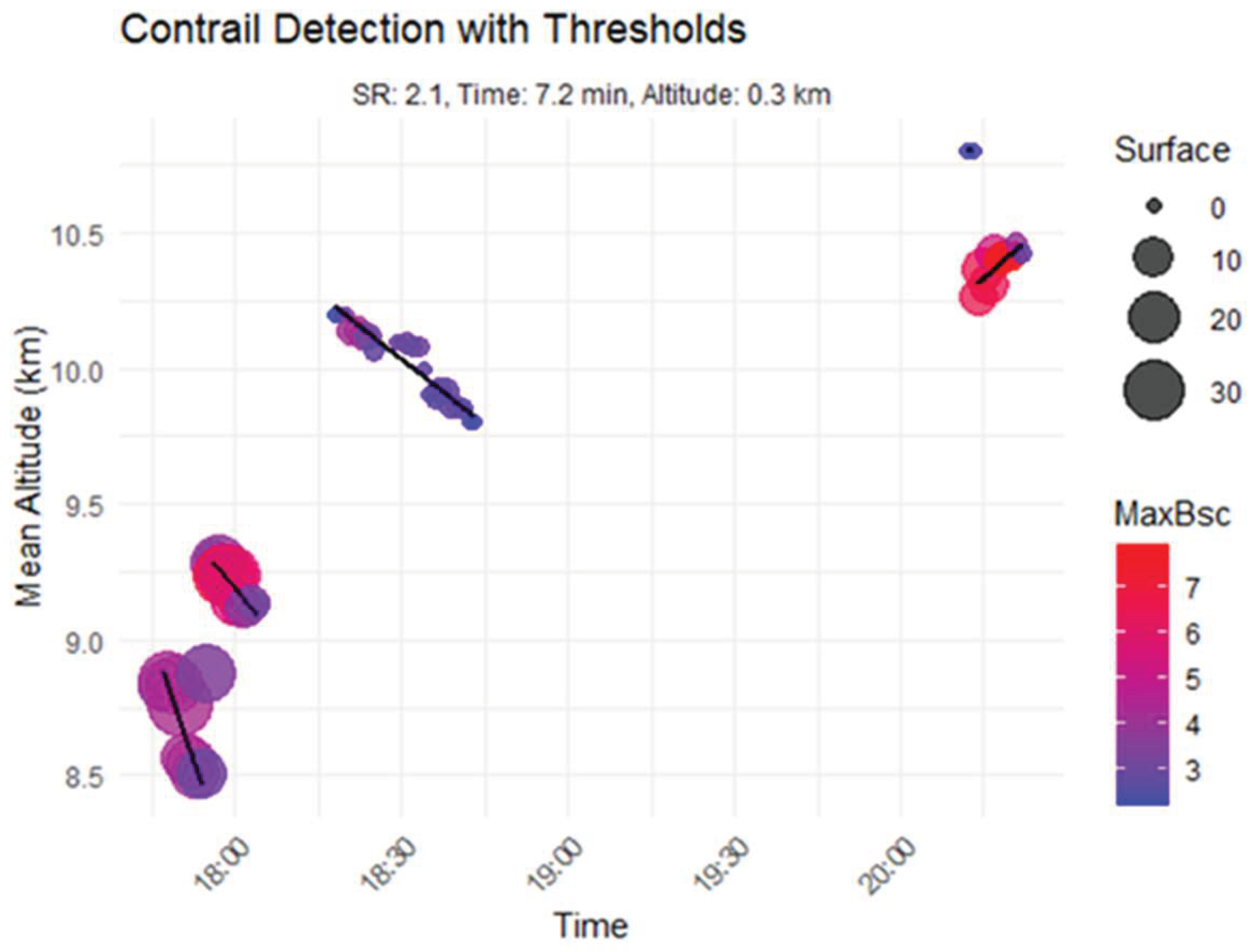
Figure 5.
Altitude-resolved profiles of the lidar scattering ratio (SR) during 03.05.2022 (case 5). Young contrail event at 20:52, under cloudy conditions, is indicated by an arrow.
Figure 5.
Altitude-resolved profiles of the lidar scattering ratio (SR) during 03.05.2022 (case 5). Young contrail event at 20:52, under cloudy conditions, is indicated by an arrow.
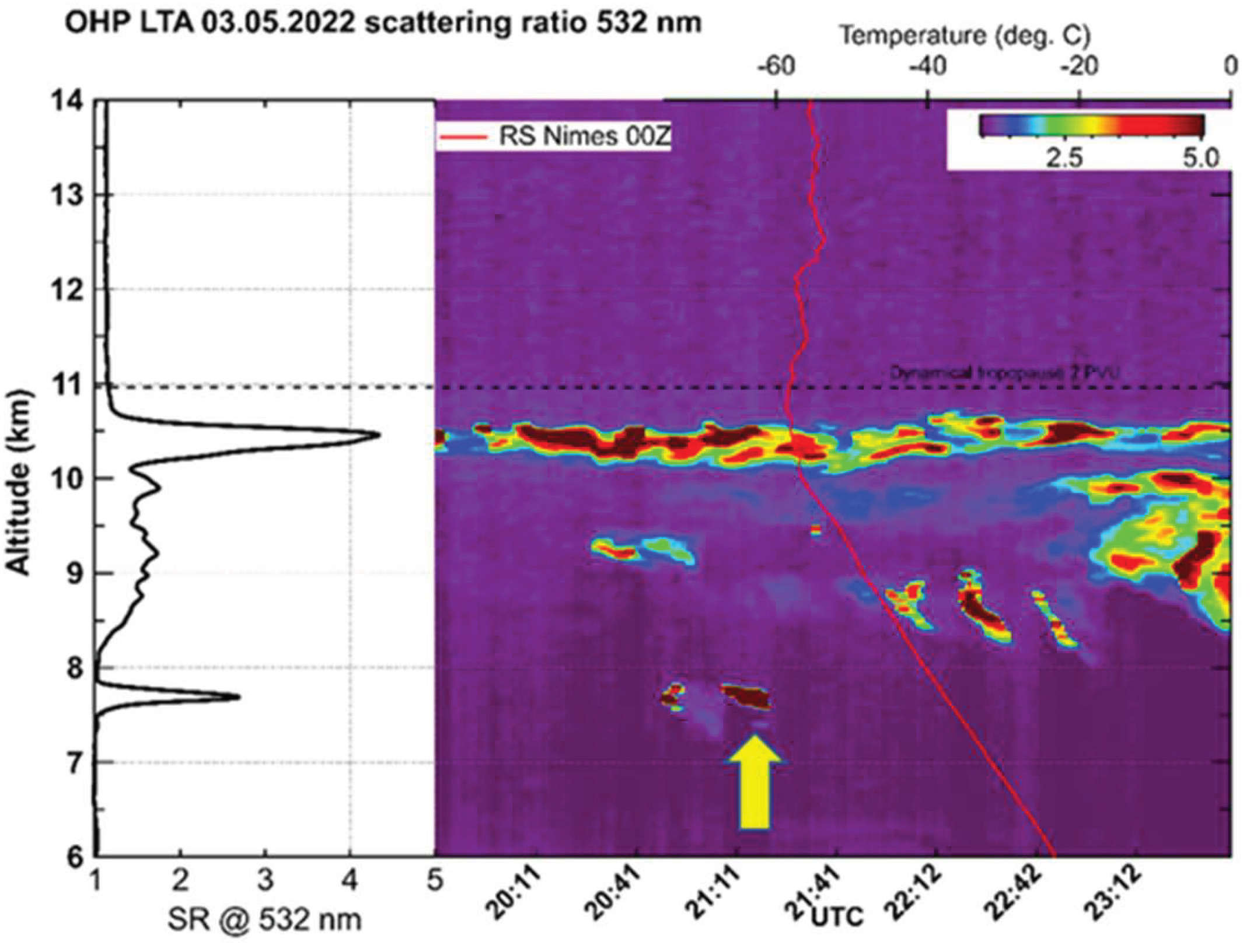
Figure 6.
Altitude-resolved profiles of the lidar scattering ratio (SR) during 25.11.2022. Two potentially contrail signatures at 20:05 (case 6) and 20:36 (case 7), under cloud-free conditions are indicated by arrows.
Figure 6.
Altitude-resolved profiles of the lidar scattering ratio (SR) during 25.11.2022. Two potentially contrail signatures at 20:05 (case 6) and 20:36 (case 7), under cloud-free conditions are indicated by arrows.
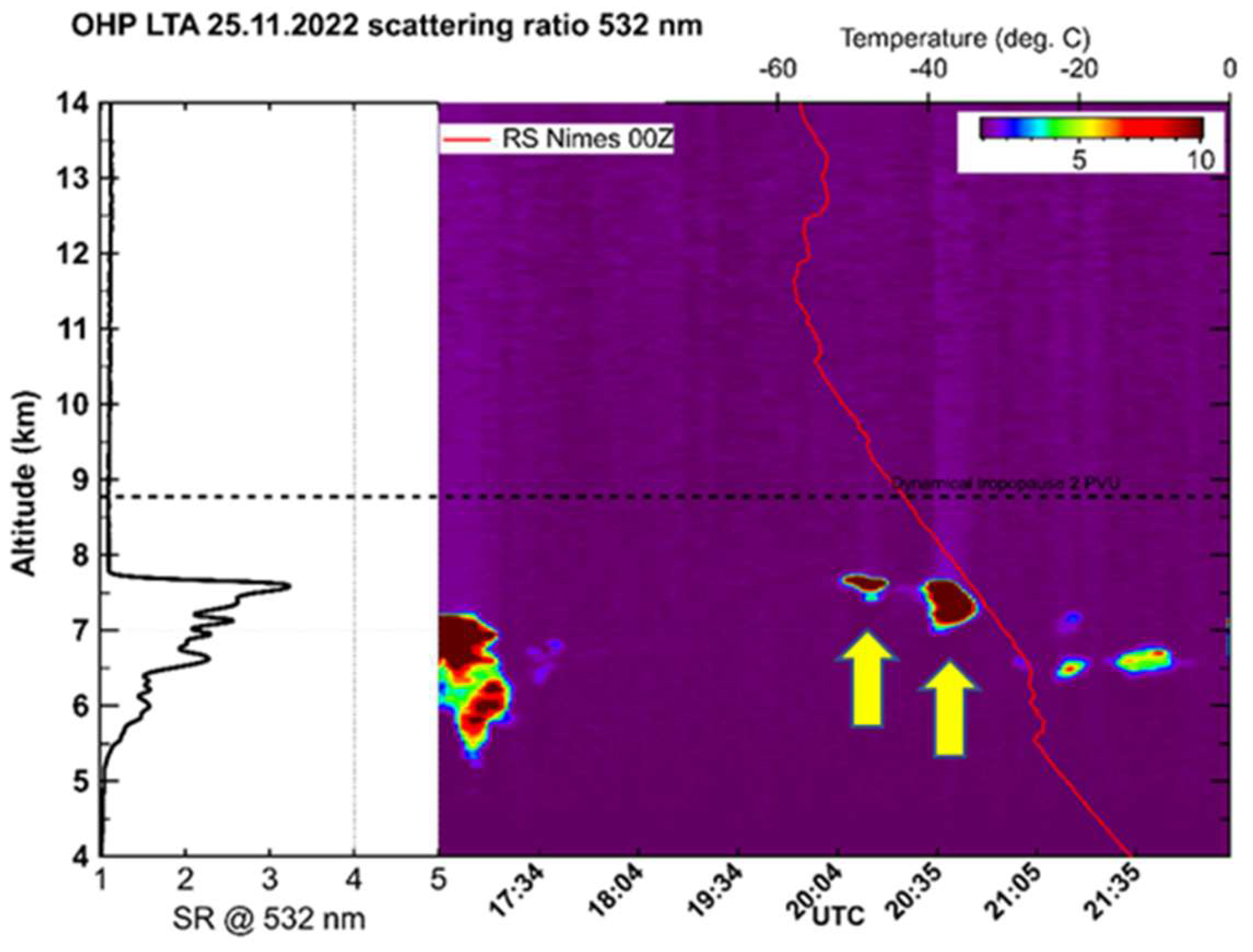
Figure 7.
Network correlation diagram of the contrail geometrical and optical properties, taking into account only the first five PC cases. Here, the mean altitude, maximal backscattering ratio, geometrical thickness, duration, orientation and their optical depth have been investigated. The nodes represent the variables and the edges represent the magnitudes of correlations.
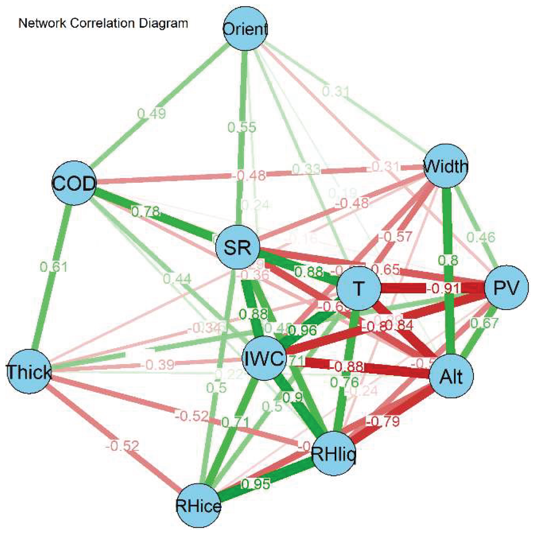
Table 1.
Categorization of contrails based on their stage of development. Different nomenclatures have been used to classify contrails by their age.
Table 1.
Categorization of contrails based on their stage of development. Different nomenclatures have been used to classify contrails by their age.
| Lifespan | Maturity | Persistence | Age | Width | Shape | Edges |
|---|---|---|---|---|---|---|
| short-lived | young | fresh | < 10 min | > 3 km | linear | sharp |
| long-lived | mature | persistent | < 1 h | > 7 km | linear | diffusive |
| old | spreading | > 1 h | > 21 km | non-linear | diffusive |
Table 3.
Mean parameters of each identified four aggregated cases during 13.01.2023. Altitude gives the contrail mean altitude. Maximal values of scattering ratio (SRmax) indicate the density of the contrails. Contrail’s geometrical thickness is calculated as the maximal vertical extend on the contrail’s cross section. Contrail’s width is calculated by multiplying the time frame of the contrail's lidar measurement by the perpendicular wind projection to the contrail principal axis. Orientation of the contrails is calculated as the slopes of their principal axes. In addition, IWC represents ice water content, and PV the potential vorticity over the contrail’s surroundings. The last column shows the contrail group, according to their formation and persistence criteria, which in these four cases belong to persistent contrails (PC).
| Geometrical/optical parameters | Thermodynamic parameters | |||||||||||
|---|---|---|---|---|---|---|---|---|---|---|---|---|
| Case | Alt. (Km) |
SRmax | Thick. (Km) |
Width (Km) |
Orient. (10-3) |
COD | T (oC) |
RHliq (%) |
RHice (%) |
PV (K·m²·kg⁻¹·s⁻¹) |
IWC (kg·m−3) |
Gr. |
| 1 | 8.7 | 4.4 | 0.6 | 2 | -1.1 | 0.10 | -56.7 | 74.8 | 108.8 | 2E-06 | 4.0E-7 | PC |
| 2 | 9.2 | 7.4 | 1.1 | 9 | -0.4 | 0.35 | -60.3 | 84.5 | 126.9 | 4E-06 | 4.0E-7 | PC |
| 3 | 10.0 | 4.2 | 0.1 | 28 | -0.3 | 0.05 | -60.4 | 89.7 | 134.6 | 3E-06 | 1.0E-7 | PC |
| 4 | 10.3 | 7.9 | 0.8 | 18 | 0.9 | 0.28 | -55.8 | 69.9 | 101.2 | 2E-06 | 1.0E-7 | PC |
Table 4.
Similar to Table 3, the geometrical, optical and thermodynamic parameters for other three cases are presented. The case 5 occurred on 03.03.2022, while the other two cases occurred on 25.11.2022. Case 5 shows a persistent contrail (PC), while cases 6 and 7 show two no-contrail events (NoC).
| Geometrical/optical parameters | Thermodynamic parameters | |||||||||||
|---|---|---|---|---|---|---|---|---|---|---|---|---|
| Case | Alt. (Km) |
SRmax | Thick. (Km) |
Width (Km) |
Orient. (10-3) |
COD | T (oC) |
RHliq (%) |
RHice (%) |
PV (K·m²·kg⁻¹·s⁻¹) |
IWC (kg·m−3) |
Gr. |
| 5 | 8.7 | 13 | 0.3 | 1.4 | 0.2 | 0.33 | -41.4 | 115.8 | 147.1 | 2.4e-07 | 1.8E-5 | PC |
| 6 | 6.9 | 35 | 0.3 | 10.7 | -0.1 | 0.22 | -44.3 | 28.5 | 43.6 | 3.0e-06 | 1.6E-5 | NoC |
| 7 | 6.7 | 56 | 0.7 | 13.6 | -0.2 | 0.98 | -44.3 | 28.5 | 43.6 | 3.0e-06 | 1.6E-5 | NoC |
Disclaimer/Publisher’s Note: The statements, opinions and data contained in all publications are solely those of the individual author(s) and contributor(s) and not of MDPI and/or the editor(s). MDPI and/or the editor(s) disclaim responsibility for any injury to people or property resulting from any ideas, methods, instructions or products referred to in the content. |
© 2025 by the authors. Licensee MDPI, Basel, Switzerland. This article is an open access article distributed under the terms and conditions of the Creative Commons Attribution (CC BY) license (http://creativecommons.org/licenses/by/4.0/).
Copyright: This open access article is published under a Creative Commons CC BY 4.0 license, which permit the free download, distribution, and reuse, provided that the author and preprint are cited in any reuse.


