
Submitted:
01 December 2025
Posted:
04 December 2025
You are already at the latest version
Abstract
In complex energy storage operating scenarios, batteries seldom undergo complete charge–discharge cycles required for periodic capacity calibration. Methods based on accelerated aging experiments can indicate possible aging paths; however, due to uncertainties like changing operating conditions, environmental variations, and manufacturing inconsistencies, the degradation information obtained from such experiments may not be applicable to the entire lifecycle. To address this, we develop a stage-wise state-of-health (SOH) prediction approach that combines offline training with online updating. During the offline training phase, multiple single-cell experiments were conducted under various combinations of depth of discharge (DOD) and C-rate. Multi-dimensional health features (HFs) were extracted and an accelerated aging probability pAA was defined. Based on the correlation statistics between HF, kHF, SOH, and pAA, all cells in the dataset were divided into general early, middle, and late aging stages. For each stage, cells were further classified by their longevity (long, medium, short), and multiple models were trained offline for each category. The results show that models trained on cells following similar aging paths achieve significantly better performance than a model trained on all data combined. Meanwhile, HF optimization was performed via a three-step process: an initial screening based on expert knowledge, a second screening using Spearman correlation coefficients, and an automatic feature importance ranking using a random forest regression (RFR) model. The proposed method offers the following innovations: (1) The stagewise multi-model strategy significantly improves SOH prediction accuracy across the entire lifecycle, maintaining the mean absolute percentage error (MAPE) within 1%. (2) The improved model provides uncertainty quantification, issuing a warning signal at least 50 cycles before the onset of accelerated aging, thereby enabling early detection of accelerating degradation. (3) Analysis of feature importance from the model outputs allows indirect identification of the primary aging mechanisms at different stages. (4) The model is robust against missing or low-quality HFs—if certain features cannot be obtained or are of poor quality, the prediction process does not fail.
Keywords:
SOH prediction
; lithium-ion battery energy storage system
; stagewise aging path
; random forest regression
1. Introduction
Lithium-ion battery energy storage systems are now widely deployed in photovoltaic, wind power integration, and grid peak-shaving applications, and the SOH is directly tied to operational safety and economic efficiency. Accurate and reliable SOH prediction is a key function of the battery management system (BMS), aiding in evaluating remaining capacity and lifetime, optimizing charge–discharge strategies to prolong service life, and preventing premature battery failures. In recent years, numerous methods for lithium-ion battery SOH estimation have been proposed, which can be broadly classified into the following categories.
(1) Direct methods based on capacity. These methods typically rely on periodic standard charge–discharge tests under constant conditions to measure the battery’s actual capacity or internal resistance for SOH evaluation. The advantage is principle simplicity and intuitive results, which can yield accurate health indicators under laboratory conditions. However, this approach requires the battery to undergo complete charge–discharge cycles or long rest tests, which is difficult to achieve in real operation. For example, Wei et al. showed that in practical applications batteries rarely experience full constant-current charge–discharge processes, making it hard to continuously perform SOH estimation based on full-cycle capacity measurements [1]. Moreover, internal resistance measurements are sensitive to state of charge and ambient temperature, so methods solely relying on capacity calibration data (e.g., full charge/discharge capacity or steady-state resistance) have limited applicability under field conditions
(2) Data-driven methods based on health feature extraction. These methods utilize easily accessible signals during battery operation (voltage, current, temperature, etc.) to extract health features, and estimate SOH through the mapping between these features and SOH [2]. Common HFs include: incremental capacity (IC) curve characteristics, where the positions and heights of peaks in the differential voltage (dV/dQ) curve during charging are analyzed to characterize changes in usable capacity [3]; voltage relaxation behavior, i.e. features of the voltage relaxation curve after charging or discharging, which reflect battery polarization and reversible capacity loss [4]; direct current resistance (DCR) evolution, where an equivalent circuit model or voltage-current transient response under operating conditions is used to obtain internal resistance growth for SOH evaluation [5]; Coulombic efficiency and capacity variance statistics; and features of the probability density function (PDF) of voltage or capacity. Studies have shown that these features can reflect internal aging mechanisms and performance degradation trends to varying degrees. For example, incremental capacity analysis has been widely used to capture internal reaction changes—Li et al. applied Gaussian smoothing to IC curves and extracted peak positions/heights to predict the SOH of high-energy NMC cells [6]. Meanwhile, many works combine the above physical features with machine learning algorithms to improve the feature-to-SOH mapping [7]. Typical algorithms include support vector machines (SVM), neural networks, and ensemble learning methods. For instance, Zhang et al. combined IC curve features with support vector regression to achieve online SOH monitoring for vehicle batteries [8]; Peng et al. used IC curve features and a back-propagation (BP) neural network to accurately predict lithium-ion battery capacity [9].
(3) Hybrid methods combining mechanism models and data-driven models. These methods integrate battery physical models (e.g., equivalent circuit models or electrochemical models) with data-driven algorithms to leverage both physical interpretability and predictive accuracy. On one hand, physical models provide a physical basis for battery aging—for example, through equivalent circuit parameters or empirical degradation formulas describing capacity fade and resistance growth; on the other hand, data-driven approaches are introduced to correct or estimate the nonlinear aspects that mechanistic models struggle to capture, thereby improving robustness and generalization [10]. Some researchers have constructed detailed electrochemical-mechanical coupled models to simulate SEI film growth and lithium plating effects on capacity fade. Dong et al. proposed a physics-based model considering both chemical and mechanical degradation mechanisms, which can simulate the SEI formation/growth process to predict capacity decay [11]; similarly, Zhuo et al. built models for active material loss and cyclable lithium loss in the electrodes, achieving accurate characterization of capacity evolution [12]. Overall, hybrid methods use physical models to provide constraints and priors, supplemented by data-driven models to correct the parts that are hard to capture, thereby enhancing the model’s adaptability to different operating conditions and battery types.
Most of the above methods have demonstrated effectiveness on simulation or laboratory datasets. However, when applying these algorithms to complex and variable real-world scenarios, many challenges remain:
(1) Uncertainty and trend identification: In actual operation, data noise, model error, and other uncertainties exist, and error distributions are not necessarily Gaussian. Most existing studies provide only a single-point SOH estimate; the few that consider error distribution often assume it to be Gaussian. Such deterministic outputs cannot reveal whether the health state is trending better or worse than expected. In other words, traditional methods struggle to promptly determine whether a battery is “degrading faster than expected” or “performing better than expected.” Recently, some researchers have introduced probabilistic approaches such as Bayesian model averaging into SOH estimation to incorporate model and parameter uncertainty, outputting a probability distribution for SOH [13]. This approach highlights that quantifying prediction uncertainty is important for early warning of abnormal aging.
(2) Lack of standard data under dynamic conditions: Field batteries operate under complex, fluctuating conditions—load power and charge/discharge rates vary frequently—making it difficult to regularly obtain complete full charge–discharge curves as SOH references. In practice, batteries often undergo only partial charge/discharge and do not reach the terminal voltages, which renders many full-cycle-based methods unusable. Thus, methods are needed that can estimate SOH from fragmented, incomplete operating data. For example, some studies have attempted to extract features from ~10-minute voltage relaxation curves or partial charge data to estimate capacity fade [14]. How to reliably extract health features and maintain model accuracy under non-standard operating profiles remains a major engineering challenge.
(3) Insufficient generalization over long-term aging and cell-to-cell differences: Different batteries, due to manufacturing variance, usage environments, and operational history, may exhibit significantly different aging trajectories. A single model is hard-pressed to cover an entire fleet of batteries over their full lifespans. On one hand, battery aging typically occurs in stages (e.g., initial, plateau, accelerated, end-of-life), with each stage governed by different degradation mechanisms and feature evolution patterns; a single model cannot easily accommodate all stages with high accuracy. On the other hand, as a battery ages, if a model trained on initial data is never updated, its error may accumulate, failing to reflect new changes in health. Additionally, in the field, cost constraints mean sensor precision is limited and data loss and noise are frequent, further complicating model deployment and long-term adaptation. Consequently, researchers have begun exploring adaptive model updating and transfer learning strategies to improve the robustness of SOH estimation during long-term operation and across different cells [15].
This paper addresses the above challenges by introducing a probabilistic characterization of SOH prediction results and a stagewise adaptive modeling approach, thereby providing new solutions for battery SOH estimation under complex real-world conditions. In Section 2, we detail the overall framework and implementation of the proposed method, including the offline multi-model training and online update strategy. Section 3 describes the experimental dataset and the extraction of health features. Section 4 evaluates the training results on the offline dataset, analyzes the aging paths captured by the models at different stages, and verifies the online application of the model under actual operating conditions through case studies. Finally, Section 5 concludes the paper.
2. Offline–Online SOH Prediction Method
Figure 1 shows the overall algorithm framework and application process. The approach comprises the following main components:
1. Data processing: After preprocessing the historical operation data, classify typical operating conditions. In general, we divide data into capacity calibration conditions and regular working conditions, and if needed, further distinguish charge and discharge phases within those.
2. Health feature extraction and screening: Extract HFs that reflect different aging stages and rates. Perform an initial HF screening based on empirical knowledge, then filter using correlation coefficients to obtain a set of HFs for model training.
3. Offline multi-model ensemble training: Quantify the correlations of HF and SOH, and and the “probability of accelerated aging” (). Based on these correlations, partition the dataset into different aging stages. Within each SOH stage, further group the data by aging rate (slow, moderate, fast), and train an improved RFR model for each group, yielding a set of models spanning multiple stages and rates. After training, use feature importance ranking to drop features with low contribution.
4. Online application: During operation, perform short-term HF prediction based on available historical data, and select the model corresponding to the current SOH stage and aging rate. Update the model with recent data under similar conditions to the battery in question, and carry out SOH predictions until the next capacity calibration test.
In the following subsections, we describe the offline training and online application processes in detail. Note that the first two feature-screening steps are relatively independent, while the final model update step relies on results from the offline training. For clarity, the feature selection procedure is discussed in a separate subsection.
2.1. Offline Multi-Model Ensemble Training
2.1.1. Automatic SOH Staging
As shown in Figure 2, battery degradation is not a linear process; generally it can be divided into an initial stage, a mild aging stage (plateau), an accelerated aging stage, and a final failure stage. The end-of-life stage usually corresponds to reaching the retirement threshold (e.g., SOH 80%). Different stages involve different aging mechanisms, HF evolution trends, and SOH decay rates, which makes it challenging for a single full-lifecycle model to maintain accuracy and robustness across all stages. Therefore, stage-specific models can better capture the aging characteristics of each phase. However, due to cell-to-cell variability, the turning points between stages are not identical for every battery, making it difficult to determine universal breakpoint values.
To quantitatively determine whether a battery has entered the accelerated aging phase, we propose a calculation method based on the aging slope, which uses global statistics and a nonlinear mapping to represent the aging trend probabilistically.
First, for each battery’s SOH–Ah curve, various smoothing and interpolation strategies are applied to reconstruct a continuous trajectory. Because aging curves differ under different conditions, we select the best-fitting scheme among polynomial fitting, Savitzky–Golay filtering, and LOWESS fitting. For any interpolated sequence we compute the discrete slope:
and take the absolute value of the slope, denoted , as a uniform measure.
Next, collect all || values from every cell over its entire life, remove abnormally high outliers, and calculate the cumulative distribution function :
Then, define a nonlinear mapping function to convert into :
where is the global mean. This mapping function ensures that in the steady-aging region (), , whereas in the accelerated-aging region (), (see Figure 3).
To account for individual differences, we recalculate a baseline slope for each battery locally. We take the average slope in the SOH range 95%–88% as a steady-state reference:
Define a slope ratio using the set of samples within a local window, we construct an empirical cumulative distribution function (ECDF):
Then define a local accelerated aging probability as:
As shown in Figure 4, for most cells increases gradually with cycling and remains at a low value, characterizing a normal slow-degradation stage; if for a particular cell rises significantly above the baseline, it means that cell has deviated from the group’s usual degradation pattern and is considered to have entered an accelerated aging stage.
This method, based on a physically interpretable SOH decay rate and combining global statistics with individual normalization, achieves a transformation from a deterministic aging rate to a probabilistic aging trend. Compared to using alone, the accelerated aging probability provides a more intuitive indication of the risk of abrupt degradation increase and maintains consistency across different cells. In early life, various HFs change markedly and have an approximately linear relationship with SOH, so HFs correlate strongly with SOH and reliably indicate overall capacity fade. However, as cycle count increases and active material loss and polarization effects accumulate, HF changes gradually saturate and some features become less sensitive to SOH. At that stage, even small fluctuations in the capacity fade can directly drive significant changes in . Utilizing this behavior, we propose a correlation-accumulation method with two thresholds to automatically segment the SOH trajectory, the core of which is to determine two breakpoints A and B (with ). Define and for any SOH subset , where denotes the correlation coefficient. First, perform a discrete search over candidate threshold set on
where ; ε> 0 is a small stabilizing term to avoid the denominator approaching zero. Next, perform a discrete search over set on :
where .
This approach eliminates the need to manually set thresholds or predefine inflection points, instead leveraging the data’s own characteristics to achieve automatic SOH stage division. It should be noted that the obtained breakpoints reflect statistical characteristics of the experimental dataset, and not every cell will adhere exactly to this pattern. If the dataset used for stage determination changes or the criteria for “capacity drop” are altered, the identified breakpoints will also shift.
2.1.2. Stagewise Multi-Rate Model Set Training
Figure 5 illustrates 17 days of operational data from an energy storage power station providing peak-shaving services. As shown, the operating profile varies day by day, leading to different aging trajectories even for the same total throughput or elapsed time. This means that using a fixed model for long-term SOH prediction can result in error accumulation, trend deviation, or misidentification of accelerated aging, severely limiting the practical value of the prediction method [16].
Additionally, due to engineering economic constraints, most energy storage systems are not equipped with high-precision sensors (for example, the voltage resolution in this dataset is 0.01 V). Such limited precision also hampers parameter identification for detailed electrochemical models and the extraction of certain features. Some common HFs may be unattainable or significantly skewed due to data loss or noise.
Therefore, a single prediction model is hard to transplant across highly variable operating conditions; even under identical conditions, differences in battery consistency make it difficult for one model to remain valid from start to finish. Thus, it is necessary to establish multiple targeted models segmented by stage and grouped by aging rate.
The specific construction is as follows: first, divide the cells into three categories (long, medium, short life) based on total lifetime. Then, for each cell, compute its (capacity fade rate) within each SOH stage identified in Section 2.1.1, and evenly divide the range of aging rates in that stage into three levels labeled “slow,” “moderate,” and “fast.” For each combination of aging stage and rate category, train one improved RFR model, thereby constructing a multi-stage, multi-rate SOH prediction model system. When a battery is in a certain life stage and exhibits a certain decay speed, there will be a corresponding model (or a closely matching model) available for use.
2.1.3. Improved RFR Algorithm Incorporating Prediction Result Probability Distribution
Generally, to address the prediction errors caused by noise and cell inconsistency, a common approach is to take the average of multiple prediction results. This method effectively captures the dominant aging trend and is easy to understand, but it overlooks the aging information contained in the distribution of the results [17]. Therefore, we optimize the RFR algorithm to retain the output distribution and extract additional insights from it.
RFR, a typical ensemble learning method, has been widely applied in battery SOH estimation. Compared to a single model, RFR offers strong nonlinear fitting capability, resistance to overfitting, and an inherent ability to evaluate feature importance [18]. A typical RFR training procedure is as follows:
(1) Bootstrap resampling: draw multiple subsamples of the training data (with replacement) to train multiple decision trees.
(2) Feature selection: for each tree, at each node split, randomly select a subset of features and choose the optimal feature from this subset, which avoids overfitting and improves generalization.
(3) Grow regression trees: each regression tree recursively partitions the data (using, e.g., CART or M5P algorithms) until certain stopping criteria are met.
(4) Ensemble aggregation: aggregate the results of all trees; traditionally, this is done by averaging the outputs of the trees.
Existing RFR models generally use the mean of the tree outputs as the final prediction. To enhance the practical reliability of SOH prediction, we introduce probability distribution modeling and data augmentation into the conventional RFR framework, proposing an improved RFR algorithm that retains the distribution information. In this improved approach, we preserve the complete set of leaf-node outputs from all decision trees, and compile the distribution of predicted SOH values for each sample. From this distribution, we extract typical statistical features including the mean, variance, and skewness. This reveals the shape of the SOH prediction distribution, reflecting the fluctuation trend of the health state and potential risks. For instance, if the output distribution is negatively skewed, it indicates a downward tendency in SOH (possibly forewarning accelerated aging); if the distribution is positively skewed, it suggests the decay rate is slowing or even a capacity recovery is possible.
Through these improvements, the proposed RFR model offers the following advantages:
(1) The prediction output is expanded from a single point value to a probabilistic interval, preserving the output distribution information. This endows the model with the ability to recognize abnormal aging behaviors such as capacity recovery or accelerated degradation, enhancing its practical utility.
(2) By integrating data augmentation and error distribution reconstruction, the model overcomes limitations of limited and non-ideal datasets, improving its robustness and adaptability in complex scenarios.
2.2. Feature Selection and Importance Ranking
HF extraction and optimization is a critical step in building an efficient and reliable prediction model. There are many factors contributing to battery SOH decline, such as operating temperature, discharge rate, number of overcharge/over-discharge events, and manufacturing defects [20]. The relationships between these factors and SOH are not one-to-one; hence even batteries with the same SOH can exhibit differences in their HFs. This uncertainty makes it very difficult to estimate SOH using any single HF. Accordingly, many studies have shown that using multiple HFs as inputs can effectively improve the accuracy and generalization of SOH estimation, reducing the uncertainty associated with any single feature being susceptible to noise, loss, or changing conditions [19]. However, increasing the number of features also significantly increases the computational burden; especially for ensemble learning algorithms like RFR, too many redundant features not only affect training and inference efficiency, but may also trigger the “curse of dimensionality,” undermining model stability.
Therefore, based on constructing a multi-dimensional HF set, we designed a three-step optimization process combining expert judgment, correlation filtering, and importance ranking to ensure that we compress the feature space as much as possible while preserving predictive performance. The steps are as follows:
2.2.1. Experience-Based Manual Screening
First, drawing on extensive research findings and preliminary experimental analysis, we initially select a set of health features that are physically interpretable and closely related to aging mechanisms. Typical features span capacity metrics, IC curve parameters, relaxation performance indices, ohmic and polarization resistances, Coulombic efficiency, temperature trends, etc. At the same time, considering the characteristics of different aging stages, we differentiate feature subsets intended for gradual aging, accelerated aging, and thermal safety warning, forming a multi-stage feature library (Table 1).
It is worth noting that many fine-grained electrochemical features, while capable of reflecting internal battery states in depth, often require strict testing conditions (e.g., constant temperature, low C-rate, extended rest) and complex computations. These are difficult to obtain frequently or compute in real-time in the field. Therefore, in engineering applications one should prioritize features that do not require special conditions, impose low computational burden, and still provide clear indications of aging.
2.2.2. Correlation Coefficient-Based Screening
Considering that the actual collected data may exhibit non-normal distributions, outliers, and multicollinearity, the traditional Pearson linear correlation has limited applicability. We employ the Spearman correlation coefficient to eliminate features with weak correlation or poor stability, thereby reducing the interference of redundant information on model performance. The Spearman coefficient is defined as [23]:
where and are the ranks of the th sample in the HF and SOH sequences respectively, and is the total number of samples. ranges from –1 to 1, with a larger absolute value indicating stronger correlation. Based on the results, we set a threshold and consider features with correlation below that threshold to be invalid features, which are removed. This step filters out features that have a weak or inconsistent relationship with SOH, thereby reducing the noise and redundancy in the model inputs.
2.2.3. Automated HF Importance Ranking Using the RFR Model
Finally, we utilize the RFR model’s built-in feature importance metric to rank the features. Random forests can measure each feature’s influence on the overall prediction by the contribution of that feature to splits in all trees. For example, in regression trees, one can define the importance of a feature by summing the total reduction in mean squared error (MSE) it contributes across all trees [24]. Specifically, if Δ is the reduction in MSE due to feature j in tree t, the importance score can be defined as the sum of those reductions over all T trees:
A larger indicates that feature contributes more to the model’s decisions. By sorting features in descending order of , we identify the most critical features and the relatively less important ones. Accordingly, lower-importance features can be further removed to simplify the model and avoid unnecessary noise. Moreover, the feature importance ranking carries physical insight: it reflects which features the model primarily relies on to assess battery health, indirectly indicating which aging mechanisms may be more dominant at that stage. For example, if in a certain stage the model’s top feature is an internal resistance metric, it may imply that aging in that stage is mainly driven by internal resistance growth; if temperature-related features rank high, one should consider the influence of thermal effects on degradation.
2.3. Online Model Update and Application
2.3.1. Short-Term HF Prediction Modeling and Application
In online SOH prediction, since the interval between two capacity calibration tests is typically long (possibly months or even longer), a key challenge is how to utilize routine operating data to evaluate SOH during these intervals. To address this, we construct a feature evolution mapping (map) model to achieve short-term HF prediction: first predicting the evolution of certain HFs, and then inferring the SOH trend from those predictions. From the experimental data, we model the aging rate of each HF under various aging paths, and use the projected charge throughput to predict the HF value at the end of a period. The main idea is illustrated in Figure 6.
As an example, Figure 7 shows the cluster of VAR curves for all cells, along with polynomial interpolation fits for those curves.
The same operating condition was repeated on two sets of cells; the mean VAR from those is calculated and found to follow a normal distribution, as shown in Figure 8.
For clarity, Figure 9 highlights a few example trajectories (paths) when VAR = 0.5. Different combinations of DOD and C-rate lead to different subsequent aging paths, and these paths are related to the current VAR value. By calculating the change slope of VAR (i.e. how VAR changes per unit Ah) for each path at VAR = 0.5, we obtain 16 slope data points (for 16 combinations of DOD and C). Plotting these as a 3D scatter and applying a two-dimensional surface interpolation yields the map shown in Figure 10.
It is apparent that larger C-rates and deeper DODs result in a higher VAR change slope. Different HFs will have their own characteristic slopes, so this mapping needs to be computed for the current value of whichever HF we use. Figure 11 shows map surfaces for three different VAR values (0.3, 0.5, 0.7); as VAR increases, the same charge throughput produces a larger change in VAR (i.e., a steeper decline in that feature).
When using the map model for prediction, we adopt an iterative rolling prediction. Using the current HF value as input, we search for all (DOD, C) pairs that correspond to the current HF and build a map for that specific HF value. From this map we obtain the short-term change rate . We then update the HF as:
where is the initial HF at the beginning of the interval, is the predicted HF, and is the forecasted charge throughput over the prediction horizon. As operation continues, the newly predicted HF becomes the starting point for the next iteration, and the prediction rolls forward. Because each iteration uses the latest HF to rebuild the map, the value of can change each step. If in practice the operating condition (DOD, C) shifts, one can directly calculate the corresponding from the map; if an untested (DOD, C) condition occurs, its effect can be obtained via interpolation on the map.
2.3.2. Offline Model Set Selection and Update
In large-scale energy storage systems, capacity test data are usually regarded as the starting point for subsequent health prediction. However, due to measurement errors, operational fluctuations, or capacity recovery effects, the SOH obtained from a capacity test often has biases, appearing as unstable local aging slopes or stagewise “bounce-back” behavior. To improve the model’s fidelity to the true aging trajectory, we propose a multi-candidate fitting approach to expand the SOH– dataset, and with it develop a more robust model selection and update mechanism.
(1) SOH–k set expansion under uncertainty: For the most recent capacity test point, let the measured capacity correspond to a health state . Using historical capacity test data , construct multiple fitting schemes (e.g., polynomial fitting, piecewise fitting, weighted smoothing) to obtain several approximate functions . For each fitting form , calculate the predicted health state at the current charge throughput :
and compute the local aging rate (slope) using the previous capacity test point:
yielding multiple candidate point pairs .
(2) Model set selection: For each candidate pair , find the model from the offline-trained model library whose training stage and aging rate are closest to these values. Collect the set of such matching models as for use in the next prediction period.
(3) Secondary training of models: Generally, different battery clusters or packs in a large energy storage station age at different paces. Incorporating information from other batteries with similar environments and aging stages into the model is an effective way to improve its accuracy. For each model in select a nearby subset of data from its original training set as follows:
where and are the central SOH and aging rate of that model’s training group, and are small tolerance margins. Retrain (or perform an incremental update on) the model using to obtain an updated model, thereby incorporating the latest aging state information of the current battery group or station cluster.
(4) Model set application: Take the multi-dimensional HFs obtained from the capacity test as the starting point, and use the map model to predict their short-term evolution. In parallel, continuously extract other HFs during normal (non-capacity-test) operation. The input feature vector thus includes both real-time measured HFs and short-term predicted HFs:
where etc. denote predicted features. Using each model, we obtain a set of SOH predictions for the current time. We analyze the SOH trend and its probability distribution to assist O&M personnel in assessing the battery health state. For the SOH distribution at each prediction time , we calculate the mean and the 5% lower confidence bound , and define their difference as an indicator of lower-tail deviation. When consistently exceeds an empirical threshold (e.g. 0.03, corresponding to a 3% SOH difference), it indicates that the lower confidence interval is shifting significantly downward, reflecting an increased left-tail risk in the prediction distribution, and an accelerated aging warning is triggered. This process is equivalent to checking the condition for several consecutive predictions to raise an alert; if subsequently falls and stays below for a certain number of cycles, the warning is lifted.
(5) Dynamic adjustment and expansion: Based on accumulated data and observed aging trends, periodically augment or prune the model library to ensure prediction reliability and system stability over long durations and evolving operating conditions.
It is worth noting that battery service life is becoming very long in practice, often over 10 years, with the vast majority of time spent in regular operation (rather than controlled tests). The proposed workflow only requires performing a model update and prediction after a new capacity test result is obtained, which greatly reduces computational demands. By selecting an appropriate model from the stagewise ensemble, long-term accumulated error is reduced, and the risk of error buildup or model failure inherent in using a single fixed model is mitigated.
3. Experimental Implementation and Data Processing
3.1. Experimental Method
The batteries tested were 50 Ah NCM622 pouch cells (manufactured by CALB). We carried out aging experiments under various combinations of depth of discharge (DOD) and C-rate, as summarized in Table 2. Four DOD levels (30%, 50%, 70%, 100%) were combined with four C-rates (1.0C, 1.2C, 1.5C, 2.0C). Each cell in Table 2 indicates two cells tested under that condition (identified by their cell numbers).
Cells were cycled under the specified conditions, and every one calendar month a performance assessment was conducted including a capacity test (full charge–discharge at low rate). Taking Cell #1 as an example, several cycles of operation are shown in Figure 12.
The operation of one full cycle for Cell #1 is illustrated in Figure 13. Regions a–e denote performance tests: specifically, capacity test, low-rate discharge, DST (Dynamic Stress Test), FUDS (Federal Urban Driving Schedule), and HPPC (Hybrid Pulse Power Characterization), respectively. Region f is the repetitive cycling under the designated aging condition. The cyclic aging phase is designed to simulate real usage where DOD is not 100%; under such conditions many HFs that depend on nearly complete charge–discharge curves cannot be obtained. Moreover, with a long span of operation without a full cycle, one cannot ascertain from routine data alone whether accelerated aging has begun in the interim.
When a cell’s capacity decayed to 80% of its rated capacity, we ended the test for that cell and marked it as reaching end-of-life. If a cell exhibited severe swelling or leakage, the experiment was immediately halted for safety. (For more detailed information, please refer to our previous work [25].)
3.2. Results and Analysis
All cells’ aging curves are plotted in Figure 14, and polynomial fits of those curves are shown in Figure 15.
Among the cells, Cell #3 had a manufacturing defect and its life was more than 40% shorter than that of Cell #4 under the same conditions; Cell #30 experienced swelling and leakage at an SOH of 0.844, terminating its test early. These two cells were excluded from subsequent analysis. As cell SOH approaches 0.8, testing frequency is usually increased for safety, to avoid bloating or leakage accidents caused by excessive cycling. We observed that low-C rate capacity tests temporarily slowed the capacity decay rate, mainly because continuous high-rate cycling causes non-uniform lithium distribution in the cell, whereas low-rate cycling with rest allows lithium to redistribute, temporarily increasing usable capacity.
Most cells did not exhibit a distinct knee point throughout their life; the accelerated aging stage was not prominent, and instead they showed an almost linear, steady decay. Such cells (for example, sample C2-DOD30-2) can be modeled quite accurately even without the stagewise prediction strategy proposed in this work. In other words, for batteries whose aging path remains smooth and linear, our method can still provide valid life predictions, but it may not demonstrate a marked advantage over traditional methods.
From the experimental data, we extracted multiple HFs at each capacity test and performance test, and conducted correlation analysis. Due to space constraints, we present only representative features from each category and report each feature’s Spearman rank correlation with SOH, as well as the correlation between its degradation rate and the capacity fade rate .
1. Capacity features: Efficiency-related indicators did not show obvious changes by the end of the experiment. Self-discharge-related metrics could not be obtained because, for the sake of accelerated testing, no prolonged rest periods were included. Therefore, the capacity features considered are primarily VAR and the capacities in specific voltage segments and .
Figure 16 and Figure 17 show the evolution of all cells’ capacity features over accumulated Ah and over SOH, respectively, and Figure 18 shows the relationship between the slopes of these features and the capacity decay rate . We observe that the VAR feature is quite sensitive to SOH changes, exhibiting a well-behaved monotonic decrease; also generally tracks the capacity fade trend; however, , having a small absolute value and showing significant changes only in later life, is strongly affected by measurement noise. Furthermore, the slopes of all three capacity features do not correlate well with the capacity fade slope . This indicates that relying solely on capacity feature slopes is insufficient to accurately characterize the aging rate, and other types of features are needed to complement them.
2. IC features:
Figure 19, Figure 20 and Figure 21 present the evolution of IC-curve features (focusing on the areas, heights, and voltage positions of the main IC peaks) for all cells. Overall, the two primary peaks of the IC curve (denoted Peak 1 and Peak 2) exhibit different aging patterns across cells. In general, one would expect all IC peaks to diminish with aging; however, in our data the first peak’s amplitude increases contrary to expectations, for which no satisfactory explanation has yet been found. Nevertheless, Peak 1’s area and height have low correlation with SOH, whereas the area and peak value of Peak 2 correlate much more strongly with SOH, making Peak 2 a more reliable indicator of capacity loss. This is likely because the electrode phase-change reaction corresponding to Peak 2 accounts for a larger fraction of the capacity, thus its attenuation is more pronounced as the cell ages. Additionally, the voltage position of Peak 1 shifts significantly lower as cycles progress, while the position of Peak 2 remains relatively stable. (A downward shift in peak voltage is another signature of aging, reflecting changes in internal resistance and reaction kinetics.)
3. Relaxation features: The relaxation process (voltage recovery after charge or discharge) reflects the extent of battery polarization (ohmic and concentration polarization) and the hysteresis of ion diffusion. When the battery is fresh, relaxation is fast and has small amplitude; as internal resistance grows and polarization worsens, the relaxation takes longer and the steady-state voltage offset increases.
Figure 22 and Figure 23 show how relaxation metrics (e.g., relaxation time and voltage drop at various SOC levels) evolve with Ah and SOH, and Figure 24 shows how the slopes of these metrics relate to . Interestingly, the relaxation time initially increases with cycling and later decreases, exhibiting a non-monotonic “rise-then-fall” behavior. A possible explanation is that from early to mid-life, SEI growth and side reactions cause polarization to increase, lengthening relaxation time and increasing its magnitude; but in the later severe aging stage, a large loss of cyclable lithium and active material sharply reduces capacity, which in turn lowers the absolute current stress (for a given C-rate), so the relaxation curve changes become slower or even somewhat mitigated. Thus, after peaking around mid-life, the relaxation metrics actually show some decline in the final stage. Additionally, differences in relaxation behavior at various SOCs provide further insight—for instance, relaxation at high SOC is typically slower and larger in magnitude because polarization is greater when the cell is near full charge; at low SOC (near end-of-discharge) the relaxation amplitude is also relatively large due to the cell being close to depletion. Overall, relaxation features capture the accumulated effects of internal resistance and diffusion impedance (peaking in mid-life), and they carry useful indications of the aging status.
4. Impedance/resistance features: These include resistances obtained from HPPC tests at various SOC levels (ohmic resistance and polarization resistance ), as well as the equivalent DC resistance (DCR) inferred from current step events during operation. (Note that DCR can be extracted under normal operating conditions, but because the current step often begins from a non-zero load current in the field, the measured value is lower than the standard test value.).
The various internal resistance features generally exhibit a trend of initially decreasing slightly and then increasing, with a significant rise observed near the end of life.
Figure 25, Figure 26 and Figure 27 plot the ohmic and polarization resistances of all cells versus Ah, versus SOH, and versus , respectively. In general, all types of internal resistance initially decrease slightly (possibly due to electrolyte wetting or SEI stabilization) and then increase, with a marked rise as the cell approaches end of life. To more clearly illustrate the distribution of resistance at different states of charge, Figure 28, Figure 29 and Figure 30 show the evolution of , , and DCR measured at SOC 20%, 40%, 50%, 60%, 80% over cycling. We observe that resistances measured at high SOC and very low SOC are relatively higher, while those at mid-level SOC (around 40%–60%) are lower and grow more slowly. This aligns with known behavior: when the cell is nearly full or nearly empty, the mechanical and concentration stresses are greater, leading to more pronounced impedance growth; at intermediate SOCs, electrode expansion/contraction is moderate and internal stress gradients are smaller, so impedance growth is more gradual [26].
Figure 31 compares the DCR measured under a standard capacity test at 80% SOC (purple curve) with the DCR estimated under actual partial usage at ~80% SOC (yellow curve). It can be seen that the in-operation DCR is slightly lower than the standard-test DCR. This is because in real operation, the current step occurs without fully resting the battery to equilibrium, so the initial voltage drop mainly reflects instantaneous ohmic resistance, yielding a somewhat lower value than the composite resistance measured under fully relaxed conditions.

Table 3.
Summary of correlations between health features and SOH metrics.
| k_HF | k_VARs | k_Qec | k_Qsc | k_IC_Area1 | k_IC_Area2 | k_IC_Peak1 |
| 0.688 | -0.532 | -0.572 | 0.390 | -0.810 | 0.375 | |
| k_IC_Peak2 | k_IC_Voltage1 | k_IC_Voltage2 | k_relaxation_time_20 | k_relaxation_time_40 | k_relaxation_time_50 | |
| -0.723 | 0.446 | 0.299 | -0.012 | -0.030 | -0.038 | |
| k_relaxation_time_60 | k_relaxation_time_80 | k_R_ohms_20 | k_R_ohms_40 | k_R_ohms_50 | k_R_ohms_60 | |
| -0.026 | 0.014 | 0.214 | 0.193 | 0.207 | 0.228 | |
| k_R_ohms_80 | k_R_ps_20 | k_R_ps_40 | k_R_ps_50 | k_R_ps_60 | k_R_ps_80 | |
| 0.190 | 0.209 | 0.208 | 0.200 | 0.205 | 0.211 | |
| HF | VARs | Qec | Qsc | IC_Area1 | IC_Area2 | IC_Peak1 |
| -0.987 | 0.662 | 0.968 | -0.934 | 0.990 | -0.910 | |
| IC_Peak2 | IC_Voltage1 | IC_Voltage2 | relaxation_time_20 | relaxation_time_40 | relaxation_time_50 | |
| 0.981 | -0.742 | -0.344 | 0.684 | 0.792 | 0.813 | |
| relaxation_time_60 | relaxation_time_80 | R_ohms_20 | R_ohms_40 | R_ohms_50 | R_ohms_60 | |
| 0.802 | 0.654 | -0.638 | -0.759 | -0.750 | -0.725 | |
| R_ohms_80 | R_ps_20 | R_ps_40 | R_ps_50 | R_ps_60 | R_ps_80 | |
| -0.607 | -0.793 | -0.833 | -0.842 | -0.829 | -0.759 | |
| DCRs_20 | DCRs_40 | DCRs_50 | DCRs_60 | DCRs_80 | - | |
| -0.700 | -0.778 | -0.792 | -0.761 | -0.660 | - |
4. Results of Model Training and Application
4.1. Offline Model Performance Evaluation
Following the methodology of Section 2.1, we conducted stagewise, multi-model offline training. First, using polynomial fitting and smoothing techniques, we interpolated each cell’s discrete SOH and HF data to construct a more densely-sampled training set. Next, using the stage partitioning criteria from Section 2.1.1, the training dataset was divided into three aging stages. The cumulative correlation ratios (as defined in Section 2.1.1) for determining stage breakpoints are plotted in Figure 32, which indicates global inflection points at A = 0.90 and B = 0.82.
For each stage, we further grouped the data into three subsets by aging rate according to the method of Section 2.1.2. We randomly selected one cell from each rate group as a test sample (C2-DOD50-2, C1-DOD70-1, C1.2-DOD30-1, representing long, medium, and short life cases, respectively) to evaluate the method’s online application performance; these cells’ data were not used in training. Because the number of samples within each stage is limited, the “fast/medium/slow” rate grouping was done by dividing the values for that stage into three ranges of equal frequency (using that stage’s 33rd and 67th percentiles as thresholds). In total, 9 model subsets were obtained, each containing data from a certain set of cells/time points. The model numbering is shown in Table 4.
Each model was trained only on its subset’s data, with a portion of each subset held out for evaluation. The models used 100 decision trees; the maximum tree depth, minimum leaf samples, and other hyperparameters were determined via RandomizedSearchCV method to balance accuracy and computational speed.
Figure 33, Figure 34 and Figure 35 show the SOH estimation results and feature importance rankings for representative models from the early stage (Model 3), middle stage (Model 5), and late stage (Model 8) on their respective test cells.
1. High-SOH (early) stage:
At the beginning of life, the model relies most on the area of the second IC peak (IC_Area2), followed by the height of the second peak (IC_Peak2). This indicates that in the initial stage, features of the second peak of the incremental capacity curve during charging are the most sensitive to SOH. Early capacity fade is predominantly controlled by loss of cyclable lithium (e.g., initial SEI formation consuming Li+). Internal-resistance-related features contribute negligibly at this stage, consistent with the fact that internal resistance growth is very slow early on and not yet limiting capacity.
2. Middle stage:
IC_Area2 still ranks first, but VAR has jumped to the most important feature; in addition, the Peak 2 height, Peak 1 area, and several resistance features (e.g., ohmic resistance at 60% SOC, polarization resistance at 80% SOC) enter the top five. This suggests that by mid-life, capacity fade is transitioning to being co-driven by active material loss and increasing internal resistance. On one hand, the VAR feature reflects changes in the overall shape of the charge curve, indicating that the distortion of the charge/discharge voltage profile is worsening (implying changes in electrode porosity structure and reversible capacity); on the other hand, resistance features begin to assume significant importance, indicating that by the middle stage the polarization impedance has risen enough to noticeably affect capacity. Mid-life degradation is thus a process jointly dominated by active material loss and resistance growth [27].
3. Low-SOH (late) stage:
In the final life stage, the derivative of IC_Area2 (k_IC_Area2) appears among the top five features, indicating the model is now leveraging not only the absolute values of peaks but also their rates of decline to judge the aging trend. Relaxation time features also gain some weight, suggesting that towards end-of-life, failure mechanisms like lithium plating and current collector corrosion may emerge, manifested by a sudden capacity drop accompanied by sharply rising polarization. Among resistance features, polarization resistance metrics rank higher than ohmic resistance, implying that in the low-SOH region the aging is mainly governed by diffusion limitations and double-layer polarization processes. In sum, the late-stage model relies on a more diverse array of features, including direct capacity-loss indicators as well as indirect indicators of accelerated degradation kinetics.
To further understand each model’s decision basis, we extracted the feature importance rankings for the representative model of each stage. In summary, the top features for the stage-specific models (in order of cumulative importance for that stage) are as follows:
(1.0, 0.9): IC_Area2, IC_Peak2; (0.9, 0.82): IC_Area2, VARs, IC_Peak2, IC_Area1, R_ohms_60, R_ps_80, R_ps_40, R_ps_20, Qsc, R_ohms_20, R_ps_60, k_IC_Peak2, R_ps_50; (0.82, 0): IC_Area2, VARs, IC_Area1, k_IC_Area2, IC_Peak2, R_ps_60, R_ps_20, R_ps_40, Qsc, R_ps_80, relaxation_time_50, R_ohms_20, relaxation_time_60, Qec.
Clearly, the models in different stages depend on features very differently. Early life degradation is mainly driven by reversible lithium loss (SEI layer formation), mid-life shifts towards a combination of active material loss and impedance growth, and late life may see sudden mechanisms like lithium plating becoming dominant. Notably, IC_Area2 shows extremely high predictive value in all stages, but extracting IC curve features like IC_Area2 requires low-C rate standard charge–discharge tests, which may not always be available in field applications. If a full IC curve cannot be obtained, the VAR feature can serve as a substitute—essentially, VAR captures how much the charging voltage curve shape deviates from that of a fresh battery, thereby conglomerating multiple aging effects to some extent.
4.2. Online Application Case Studies
We selected three cells (one from each life category) to demonstrate the online prediction performance. Figure 36, Figure 37 and Figure 38 show the SOH prediction results and the evolution of their predicted probability distributions after each capacity test over the entire life of each cell.
The results indicate that the stagewise models achieve high prediction accuracy for cells with different aging characteristics: at each capacity test point, the predicted SOH mean is very close to the measured value, with MAPE within 1%. For example, for the longest-lived cell (C1.2-DOD30-1), the average error between the predicted SOH and measured SOH at each stage is under 0.5%, with a maximum error of only about 0.8%; for the medium-life cell (C1-DOD70-1), the errors are slightly above 1%; for the shortest-lived cell (C2-DOD50-2), which exhibited an abrupt change in aging rate, the prediction error is around 0.7%. Compared to using a single model without stage partitioning, our method significantly improves long-term SOH prediction accuracy and stability. In particular, in late life a single global model often underestimates the degree of degradation due to limited training data for that region, whereas the stagewise models effectively avoid this issue, keeping the cumulative error across the lifespan low.
It should be emphasized that because capacity measurements themselves have some error, pointwise prediction errors (e.g., MAPE at each test) are not the sole basis for evaluating model performance. The evolution of SOH with cycling and its predicted probability bands align more closely with the actual aging trajectory, demonstrating the model’s practical value.
In the case of cell C2-DOD50-2, the third and fourth capacity tests showed anomalous results (a slight capacity recovery), which may have misled experimenters—by the next test, SOH was already near 0.8. To avoid a safety incident, a follow-up test was conducted shortly after, confirming SOH had fallen below 0.8 and the experiment was terminated. However, with our method, a warning would have been issued before the third capacity test, prompting maintenance personnel to increase the test frequency and thus avert the risk. Additionally, looking back from later data, the SOH predicted before the third test likely reflected the true aging path more accurately than the temporarily higher measured value. In cell C1-DOD70-1, accelerated aging could only be confirmed (by a notable change in average decay slope) after the 7th capacity test, whereas our method raised an alert right after the 5th test. For cell C1.2-DOD30-1, the overall aging rate was so slow that even by the 6th capacity test it might be unclear whether aging had accelerated, but our method was continuously issuing warnings during that phase of operation.
To test the model’s resilience under data deficiencies, we performed a simulation on a sample cell (C2-DOD50-2) where we introduced feature dropouts and noise: 5% of the input data points were randomly replaced with NaN values. The results, shown in Figure 39, indicate that the predicted SOH distribution interval widens notably, but the overall trend assessment remains correct, and the early warning is only delayed by a few tens of cycles. It still provides strong guidance, demonstrating that the proposed model can tolerate a certain degree of data quality issues.
5. Conclusion
In this work, focusing on lithium-ion battery SOH estimation, we proposed a stagewise prediction method combining offline training with online updating, and validated it with experimental data. The main conclusions are summarized as follows:
1. Stagewise multi-model strategy: Segmenting the battery life into stages (initial, plateau, accelerated, etc.) and training dedicated models for different aging rates can make prediction models more targeted. With each stage’s model handling its respective segment, long-term prediction accuracy and robustness are significantly improved. The cumulative error over life is greatly reduced, especially avoiding the issue that a single model has difficulty accounting for both early and late-stage aging characteristics.
2. Improved RFR with uncertainty quantification: The improved RFR algorithm provides an uncertainty evaluation of the results, enabling trend forecasting. Traditional RFR outputs only a point estimate of SOH, whereas the improved approach retains the distribution of leaf outputs and yields a probability density for SOH. Experiments show that under complex conditions (non-Gaussian errors, accelerated aging, etc.), this probabilistic output indicates how the predicted value deviates from expectations in direction and magnitude. For example, for incipient accelerated decay, the model’s output distribution becomes significantly negatively skewed or even bimodal, giving a clear warning signal well before SOH actually plunges. This capability is extremely valuable in engineering applications, overcoming the limitation of earlier methods that could only provide a number without judging whether it was “good” or “bad.”
3. Adaptability to missing data and condition changes: By carefully selecting multi-dimensional HFs and performing correlation and importance screening, we ensured the input features are relatively independent yet complementary. On the one hand, the model will not fail if some HFs cannot be obtained or deviate abnormally; on the other hand, the importance ranking of the remaining features gives insight into the primary aging modes, allowing us to add or replace features to continuously optimize the model. Furthermore, the online model update mechanism guarantees that the model adapts as battery operating conditions evolve, avoiding the pitfall of “one model used forever”.
Areas for further research include: (1) Extension of the feature evolution map model: The short-term HF prediction model developed here is based on aging data from our tested combinations; for different manufacturers or cell chemistries, additional aging experiments are needed to enrich the spectrum of aging paths and improve the map model’s coverage. In the future, techniques like transfer learning could be explored to quickly transfer the existing model to new types of batteries. (2) Model deployment and computational efficiency: Although our method demonstrated good performance on a high-performance workstation, deploying it in an actual BMS requires consideration of computational load and memory constraints. Future work could focus on model lightweighting for embedded implementation—e.g., compressing the random forest model size or leveraging distributed computing for the probabilistic outputs—to ensure the model can operate in real time within the BMS’s limited resources.
Author Contributions
Conceptualization, W.X. and J.J.; methodology, J.J., H.X. and W.X.;software, J.J. and H.X.; validation, K.H., W.X. and W.Z.; formal analysis W.X.; investigation, J.J. and K.H.; resources, K.H., W.X. and W.Z.; writing—original draft preparation, J.J.and W.X.; writing—review and editing, J.J., W.Z. and W.X.; visualization, H.X., and J.J.; supervision, W.X. and K.H.; funding acquisition, K.H. and W.X. All authors have read and agreed to the published version of the manuscript.
Funding
This research was funded by National Natural Science Foundation of China Joint Fund (Project No.: U23B20111, Project Title: Theory of Uncertainty for High-Proportion Wind and Solar Power Sources and Grid Regulation Technology).
Data Availability Statement
The data presented in this study are available on request from the corresponding author.
Acknowledgments
Thanks to the many students, and teachers from Chongqing University who have participated in the experiment for more than three years. Thanks to the scholars mentioned in the references for their research results on health feature extraction.
Conflicts of Interest
The authors declare no conflicts of interest.
Abbreviations
The following abbreviations are used in this manuscript:
| SOH | State of Health |
| DOD | Depth of Discharge |
| HF | Health Feature |
| RFR | Random Forest Regression |
| Ah | Ampere-hour |
| VAR | Capacity variance (variance of throughput over voltage range) |
| IC | Incremental Capacity |
| IC_Area1 | Area under the first peak of the IC curve |
| IC_Area2 | Area under the second peak of the IC curve |
| IC_Peak1 | Peak value of the first peak in the IC curve |
| IC_Peak2 | Peak value of the second peak in the IC curve |
| k_IC_Area2 | Degradation rate of IC_Area2 |
| Q_sc | Capacity in semi-charged segment (voltage-based) |
| Q_ec | Capacity in end-charged segment (voltage-based) |
| DCR | Direct Current Resistance |
| R_ohm | Ohmic resistance |
| R_pol | Polarization resistance |
| HPPC | Hybrid Pulse Power Characterization |
| FUDS | Federal Urban Driving Schedule |
| Probability of Accelerated Aging | |
| SOH degradation rate (slope) | |
| Degradation rate of health feature | |
| ECDF | Empirical Cumulative Distribution Function |
| MAPE | Mean Absolute Percentage Error |
| BMS | Battery Management System |
| MAP | Feature Evolution Mapping Model |
| DST | Dynamic Stress Test |
| SEI | Solid Electrolyte Interphase |
References
- Z. Wei, H. Ruan, Y. Li, J. Li, C. Zhang, and H. He, “Multistage state of health estimation of lithium-ion battery with high tolerance to heavily partial charging,” IEEE Trans. Power Electron., vol. 37, no. 6, pp. 7432–7442, June 2022. [CrossRef]
- X. Huang et al., “Robust and generalizable lithium-ion battery health estimation using multi-scale field data decomposition and fusion,” J. Power Sources, vol. 642, p. 236939, June 2025. [CrossRef]
- J. Guo, Y. Li, J. Meng, K. Pedersen, L. Gurevich, and D.-I. Stroe, “Understanding the mechanism of capacity increase during early cycling of commercial NMC/graphite lithium-ion batteries,” J. Energy Chem., vol. 74, pp. 34–44, Nov. 2022. [CrossRef]
- “An adaptive and interpretable SOH estimation method for lithium-ion batteries based-on relaxation voltage cross-scale features and multi-LSTM-RFR2,” Energy, vol. 304, p. 132167, Sept. 2024. [CrossRef]
- R. Ibraheem, C. Strange, and G. dos Reis, “Capacity and internal resistance of lithium-ion batteries: full degradation curve prediction from voltage response at constant current at discharge,” J. Power Sources, vol. 556, p. 232477, Feb. 2023. [CrossRef]
- K. Li and N. Xie, “Battery health prognostics based on improved incremental capacity using a hybrid grey modelling and gaussian process regression,” Energy, vol. 303, p. 131888, Sept. 2024. [CrossRef]
- B. Ospina Agudelo, W. Zamboni, F. Postiglione, and E. Monmasson, “Battery state-of-health estimation based on multiple charge and discharge features,” Energy, vol. 263, p. 125637, Jan. 2023. [CrossRef]
- Y. Zhang, Y. Liu, J. Wang, and T. Zhang, “State-of-health estimation for lithium-ion batteries by combining model-based incremental capacity analysis with support vector regression,” Energy, vol. 239, p. 121986, Jan. 2022. [CrossRef]
- J. Peng et al., “State of health estimation of Li-ion battery via incremental capacity analysis and internal resistance identification based on kolmogorov–arnold networks,” Batteries, vol. 10, no. 9, p. 315, Sept. 2024. [CrossRef]
- B. Xu, J. Shi, S. Li, H. Li, and Z. Wang, “Energy consumption and battery aging minimization using a Q-learning strategy for a battery/ultracapacitor electric vehicle,” Energy, vol. 229, p. 120705, Aug. 2021. [CrossRef]
- G. Dong and J. Wei, “A physics-based aging model for lithium-ion battery with coupled chemical/mechanical degradation mechanisms,” Electrochimica Acta, vol. 395, p. 139133, Nov. 2021. [CrossRef]
- M. Zhuo, G. Offer, and M. Marinescu, “Degradation model of high-nickel positive electrodes: effects of loss of active material and cyclable lithium on capacity fade,” J. Power Sources, vol. 556, p. 232461, Feb. 2023. [CrossRef]
- Q. Zou and J. Wen, “Battery state-of-health estimation incorporating model uncertainty based on bayesian model averaging,” Energy, vol. 308, p. 132884, Nov. 2024. [CrossRef]
- X. Feng, Y. Zhang, R. Xiong, and A. Tang, “Estimating battery state of health with 10-min relaxation voltage across various charging states of charge,” Ienergy, vol. 2, no. 4, pp. 308–313, Dec. 2023. [CrossRef]
- S. Tao et al., “Generative learning assisted state-of-health estimation for sustainable battery recycling with random retirement conditions,” Nat. Commun., vol. 15, no. 1, p. 10154, Nov. 2024. [CrossRef]
- X. Li, D. Yu, S. B. Vilsen, V. R. Subramanian, and D.-I. Stroe, “Robust remaining useful lifetime prediction for lithium-ion batteries with dual gaussian process regression-based ensemble strategies on limited sample data,” IEEE Trans. Transport. Electrific., vol. 11, no. 2, pp. 6279–6290, Apr. 2025. [CrossRef]
- H. Liu et al., “Multi-modal framework for battery state of health evaluation using open-source electric vehicle data,” Nat. Commun., vol. 16, no. 1, p. 1137, Jan. 2025. [CrossRef]
- G. Wang, Z. Lyu, and X. Li, “An optimized random forest regression model for Li-ion battery prognostics and health management,” Batteries, vol. 9, no. 6, p. 332, June 2023. [CrossRef]
- Z. Shi, C. Zhu, H. Liang, S. Wang, and C. Yu, “Multiple measurement health factors extraction and transfer learning with convolutional-BiLSTM algorithm for state-of-health evaluation of energy storage batteries,” Ionics, vol. 31, no. 2, pp. 1699–1717, Feb. 2025. [CrossRef]
- H. Movahedi, S. Pannala, J. B. Siegel, and A. G. Stefanopoulou, “Physics-informed optimal experiment design of calendar aging tests and sensitivity analysis for SEI parameters estimation in lithium-ion batteries,” IFAC-Pap., vol. 56, no. 3, pp. 433–438, Jan. 2023. [CrossRef]
- W. Xiao, S. Miao, J. Jia, Q. Zhu, and Y. Huang, “Lithium-ion batteries fault diagnosis based on multi-dimensional indicator,” IET Conf. Proc., vol. 2021, no. 9, pp. 96–101, Feb. 2022. [CrossRef]
- H. Xu, J. Jia, W. Xiao, L. Hou, and Y. Shang, “A high-precision state of health estimation method based on data augmentation for large-capacity lithium-ion batteries,” J. Energy Storage, vol. 102, p. 114028, Nov. 2024. [CrossRef]
- X. He, Z. Wu, J. Bai, J. Zhu, L. Lv, and L. Wang, “A novel SOH estimation method for lithium-ion batteries based on the PSO–GWO–LSSVM prediction model with multi-dimensional health features extraction,” Appl. Sci., vol. 15, no. 7, p. 3592, Jan. 2025. [CrossRef]
- K. S. R. Mawonou, A. Eddahech, D. Dumur, D. Beauvois, and E. Godoy, “State-of-health estimators coupled to a random forest approach for lithium-ion battery aging factor ranking,” J. Power Sources, vol. 484, p. 229154, Feb. 2021. [CrossRef]
- W. Xiao et al., “A novel differentiated control strategy for an energy storage system that minimizes battery aging cost based on multiple health features,” Batteries, vol. 10, no. 4, p. 143, Apr. 2024. [CrossRef]
- S. Barcellona, S. Colnago, G. Dotelli, S. Latorrata, and L. Piegari, “Aging effect on the variation of Li-ion battery resistance as function of temperature and state of charge,” J. Energy Storage, vol. 50, p. 104658, June 2022. [CrossRef]
- C. Fan, X. Tian, and C. Gu, “Perturbation-based battery impedance characterization methods: from the laboratory to practical implementation,” Batteries, vol. 10, no. 12, p. 414, Dec. 2024. [CrossRef]
Figure 1.
Algorithmic framework and workflow of the proposed SOH prediction method.
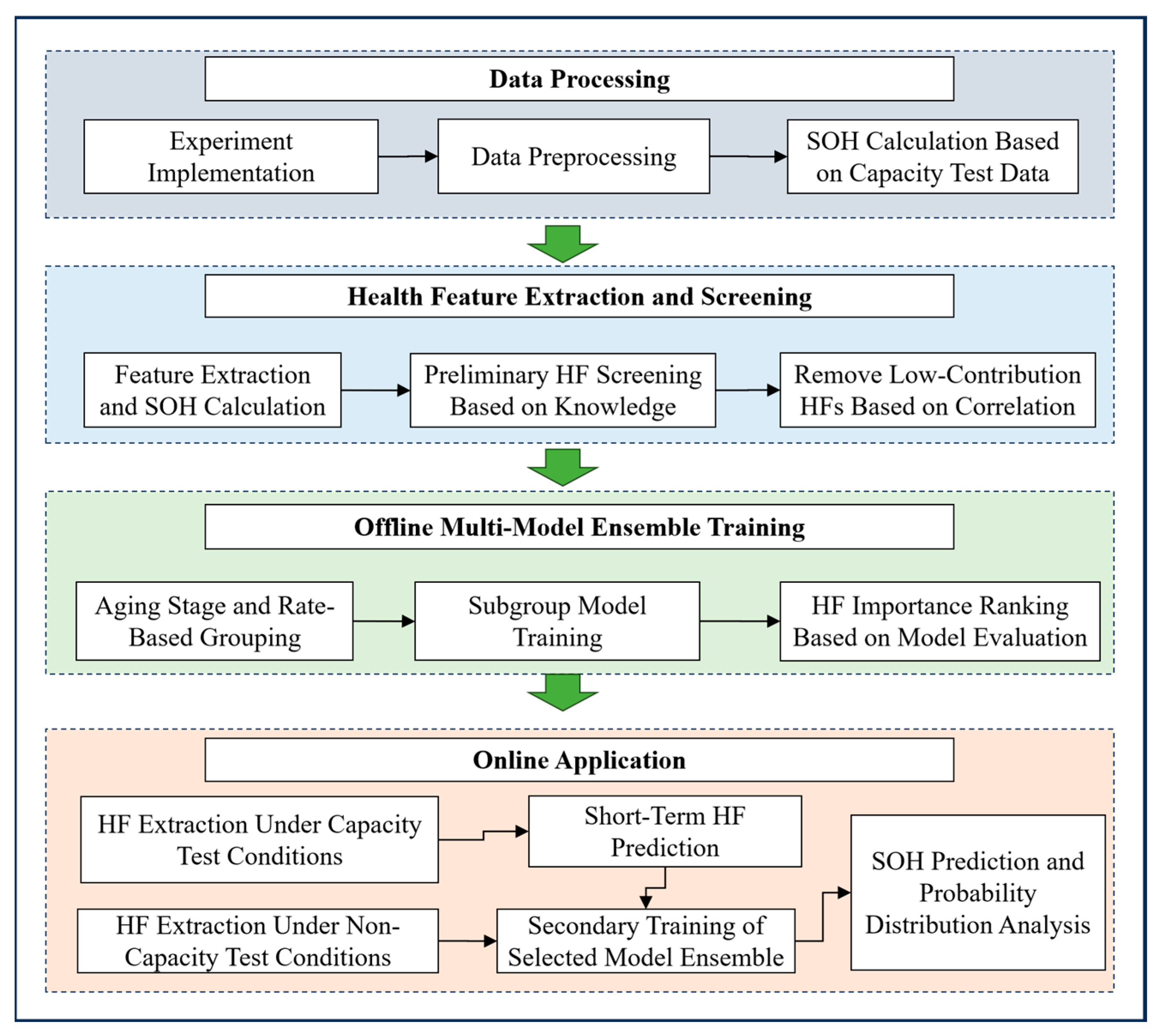
Figure 2.
a typical segmented aging curve.
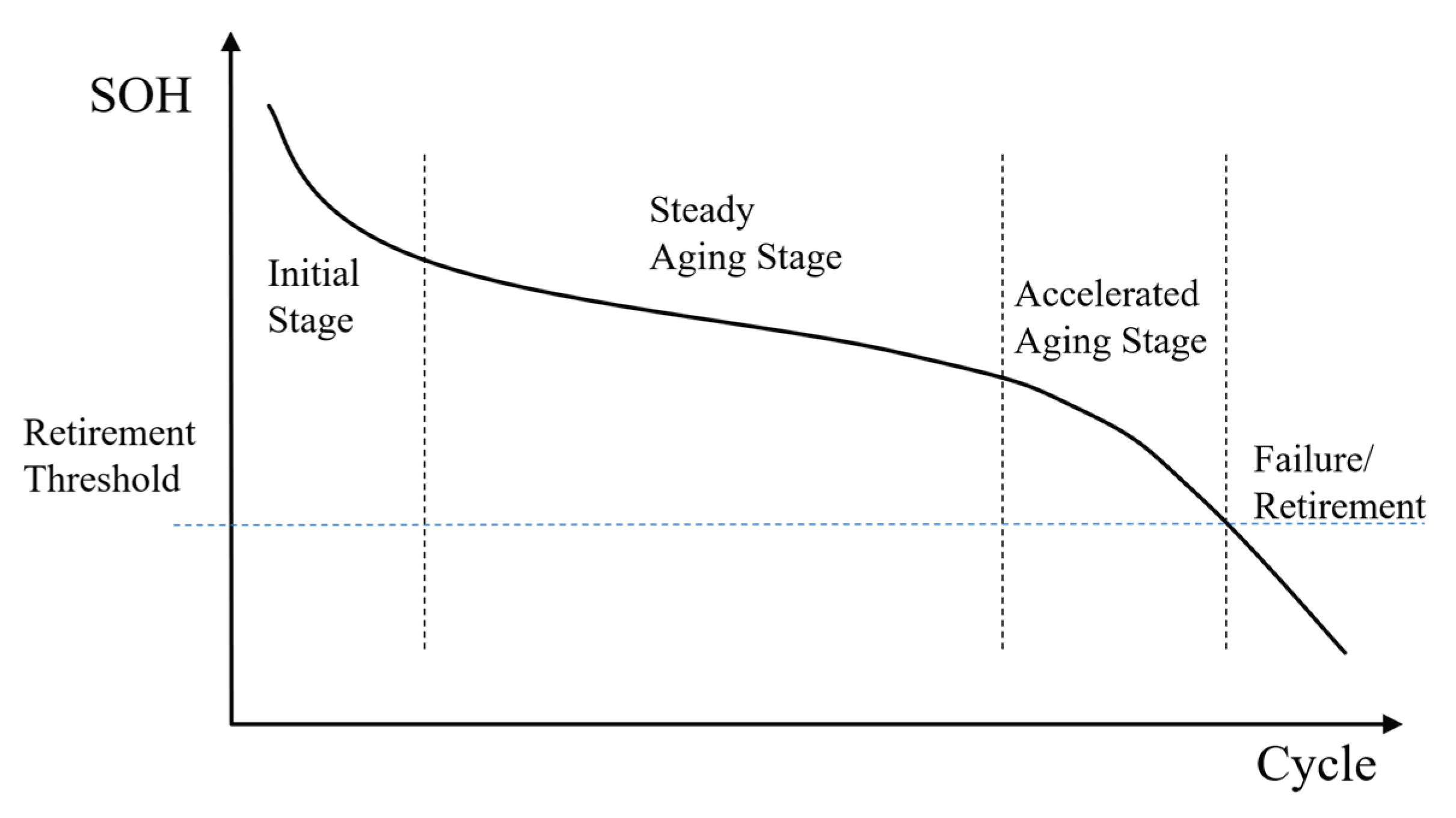
Figure 3.
Probability density distribution of and the mapping relationship of .
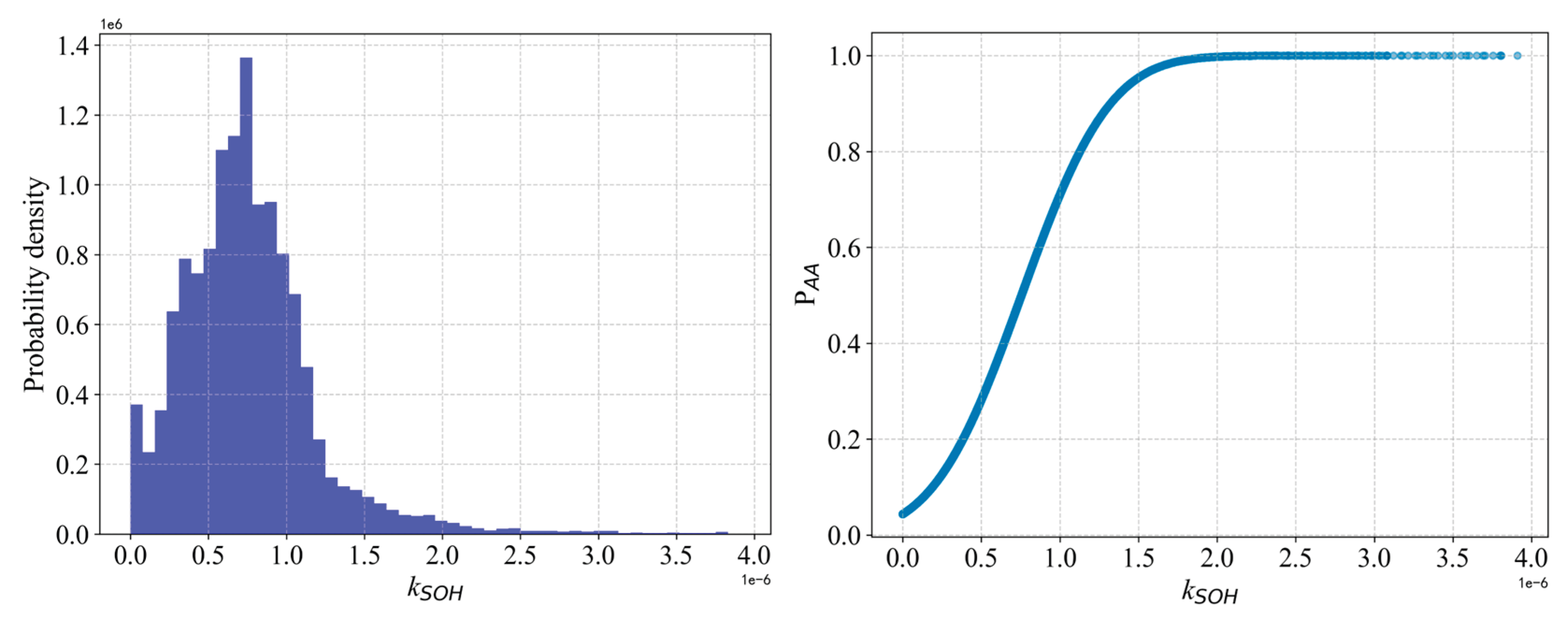
Figure 4.
Probability density distribution of and the mapping relationship of .
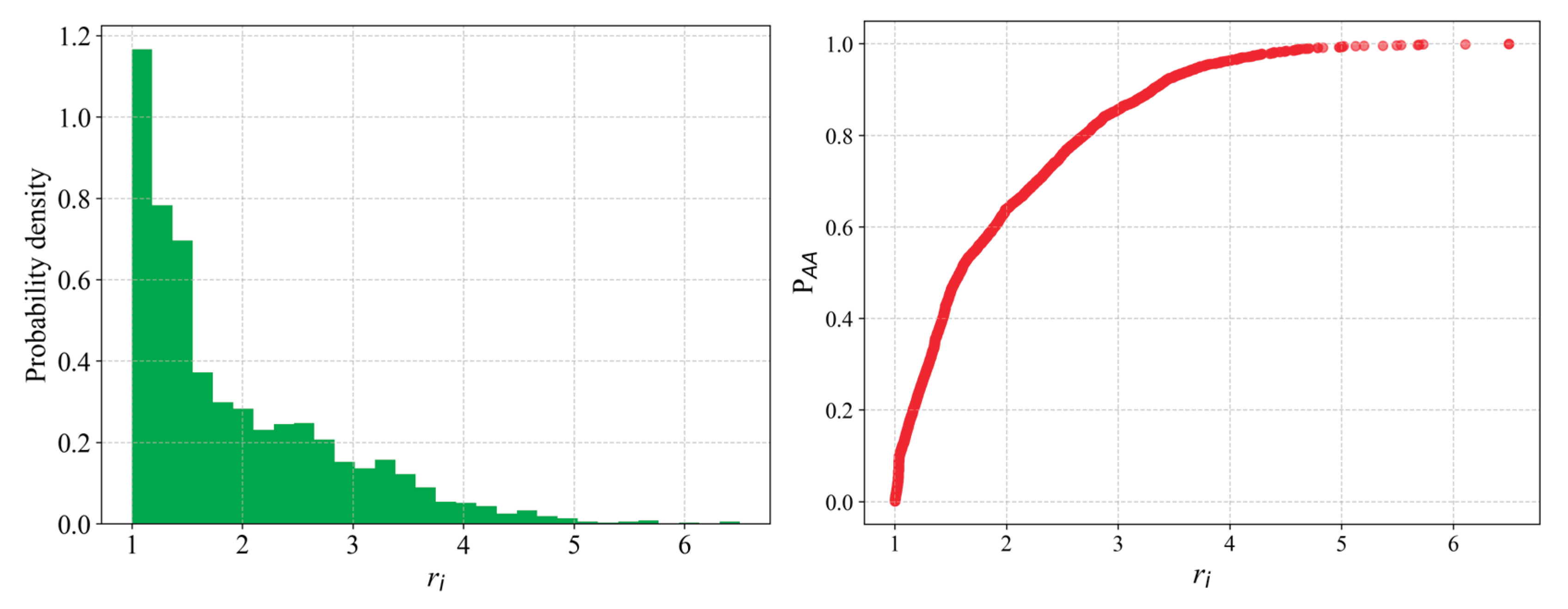
Figure 5.
Operational data from a representative energy storage power station.
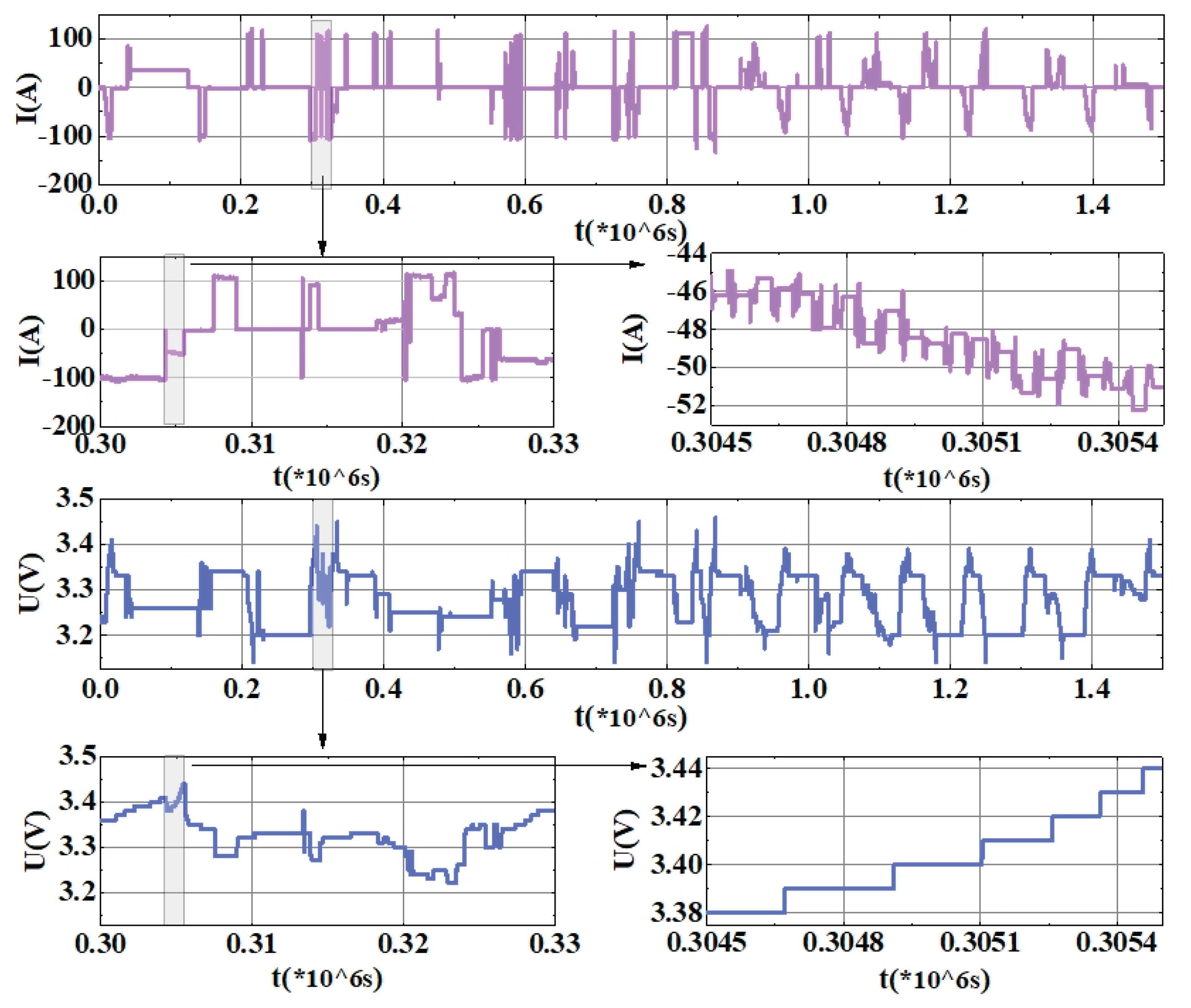
Figure 6.
Illustration of the HF Prediction Procedure.
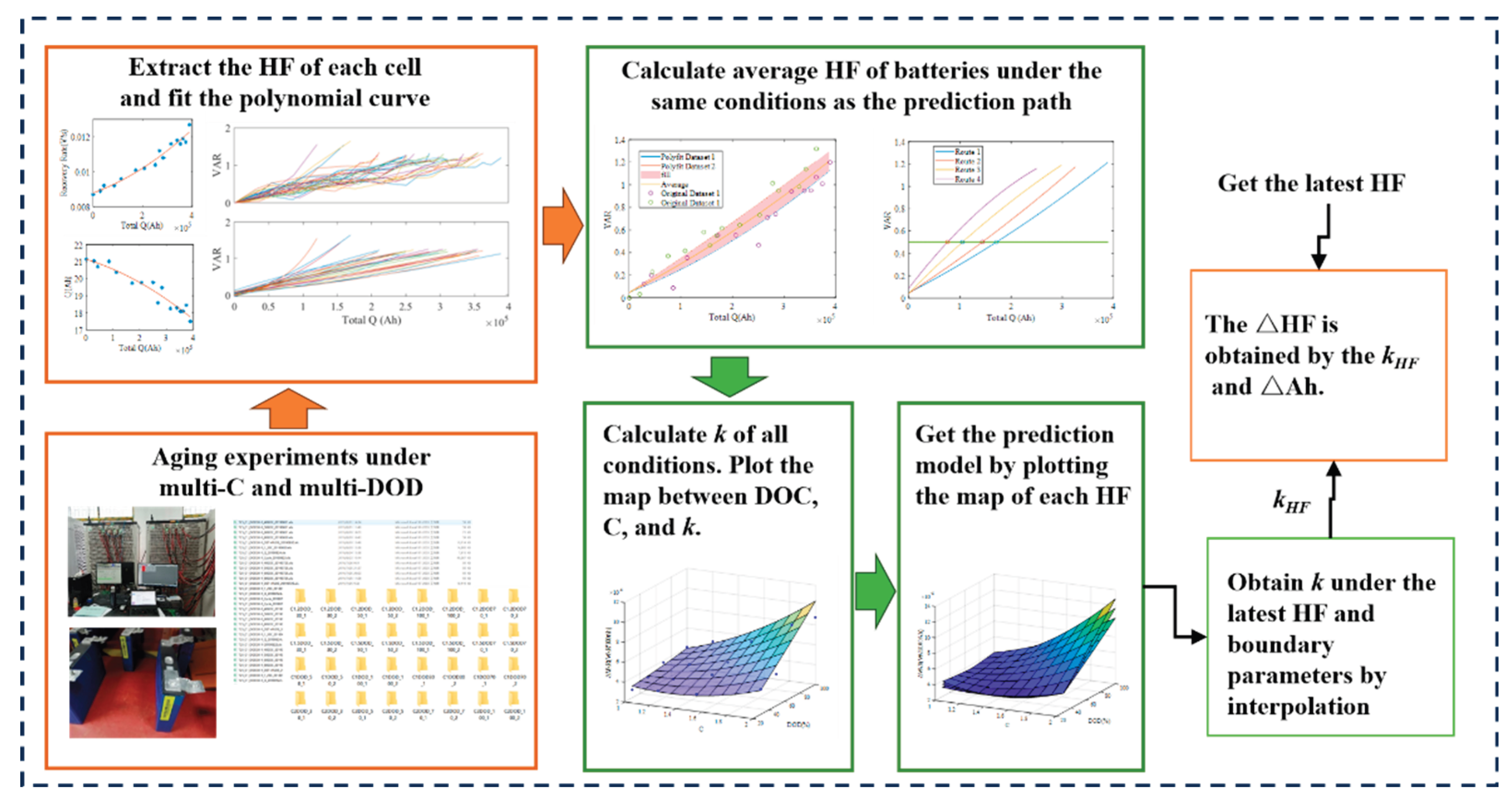
Figure 7.
Original and fitted VAR curves.
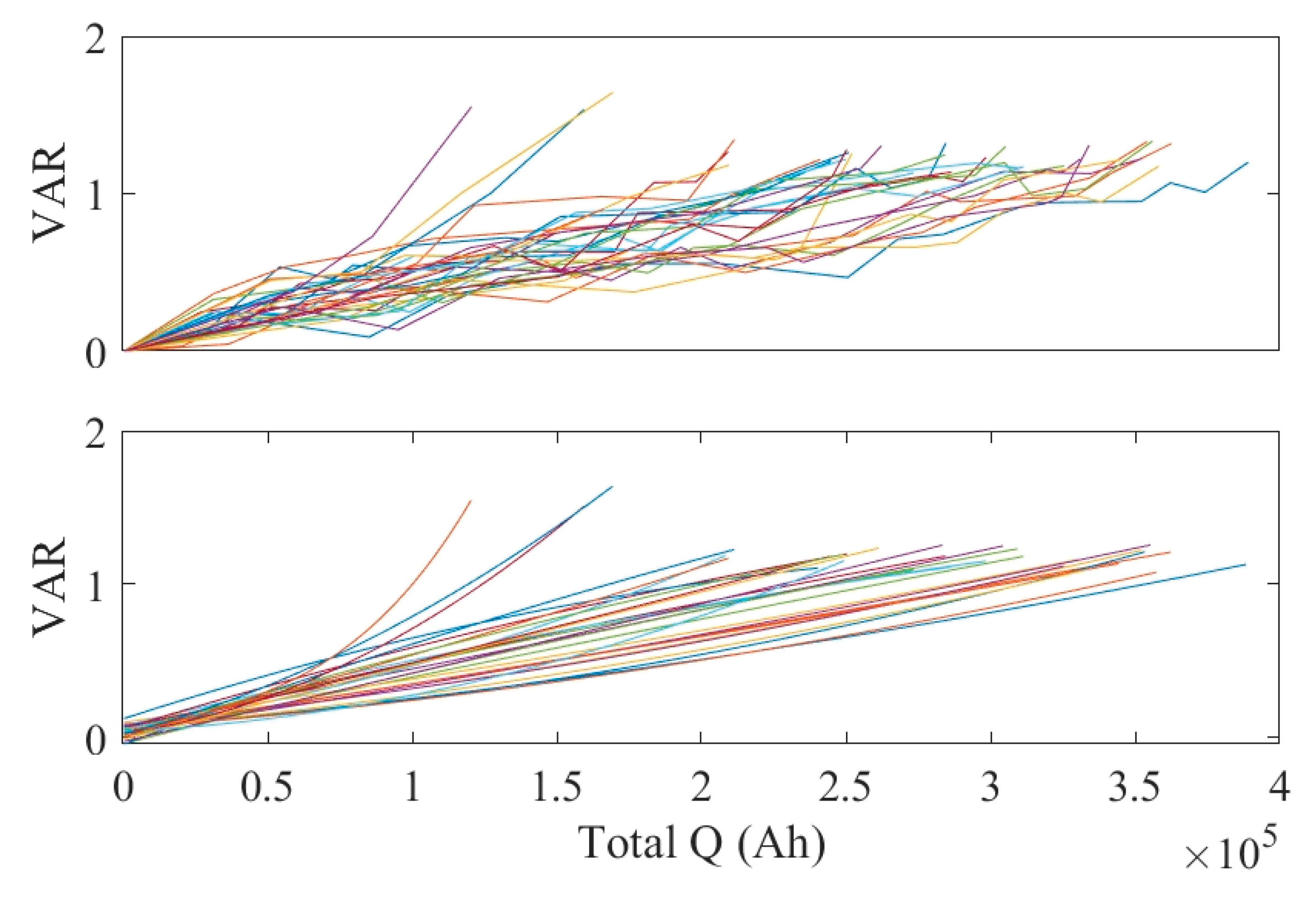
Figure 8.
Statistical distribution of calculated VARs for two batteries;.
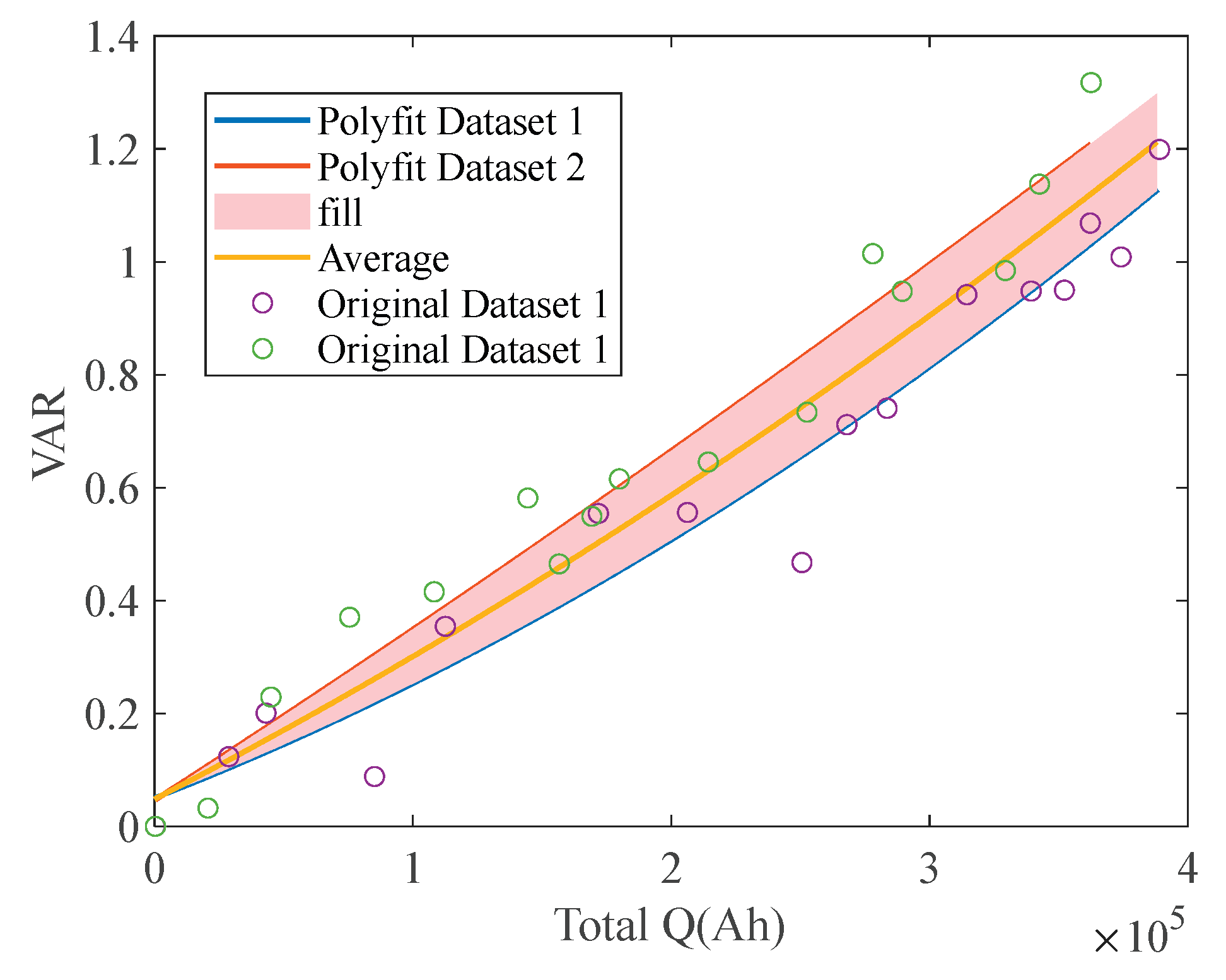
Figure 9.
Schematic diagram of multiple paths with VAR = 0.5.
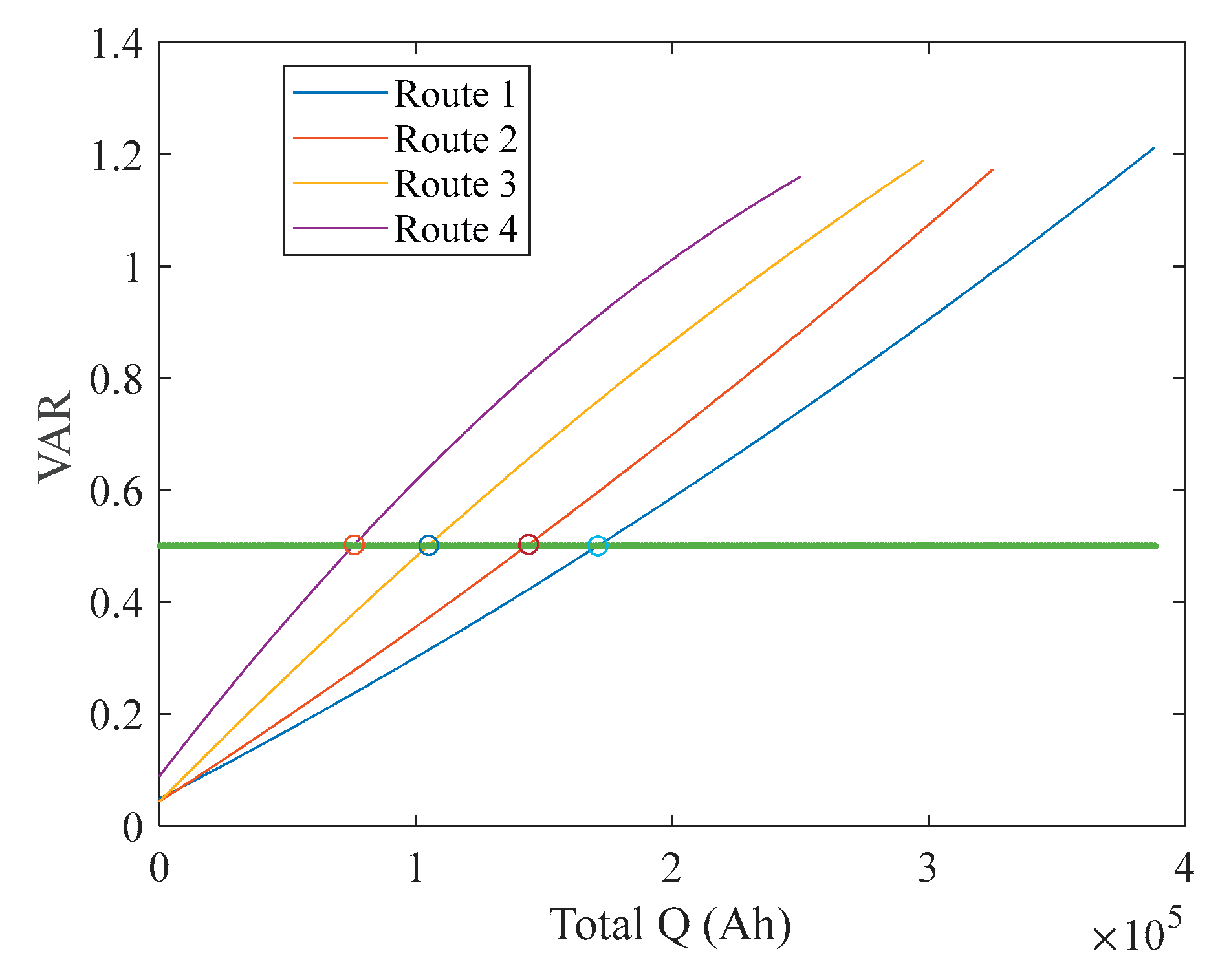
Figure 10.
Map of C, DOD, and k with VAR=0.5.
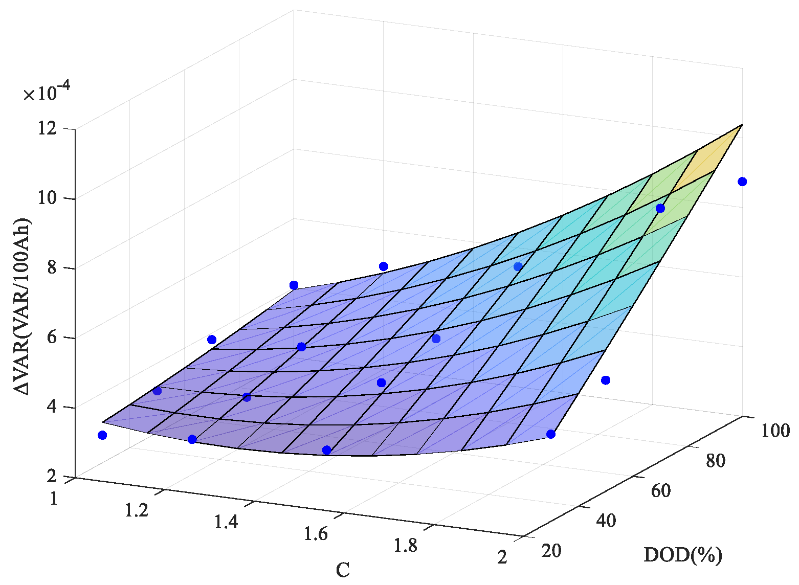
Figure 11.
Map of C, DOD, and k with VAR=0.3, 0.5, and 0.7.
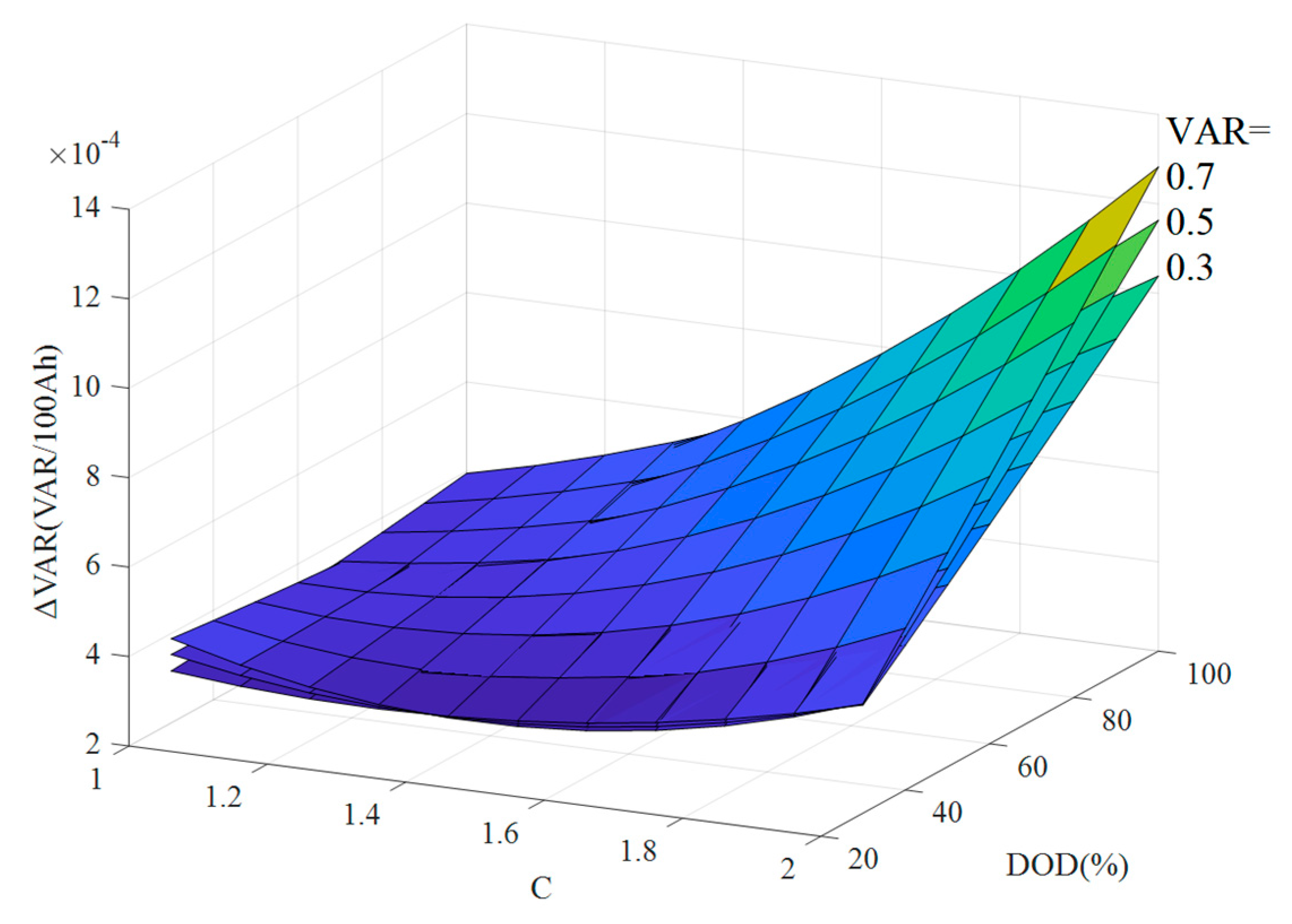
Figure 12.
Partial test profile of Cell #1: (a) current; (b) voltage.
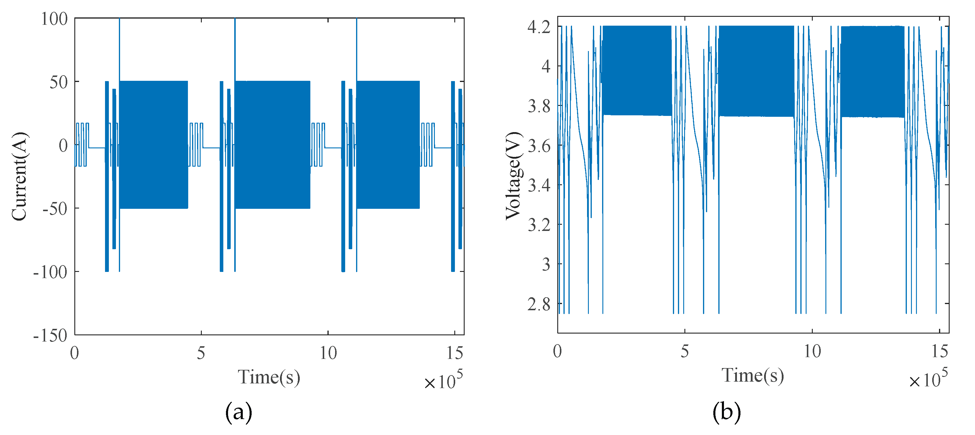
Figure 13.
One test cycle of Cell #1 (performance tests a–e, aging cycles f).
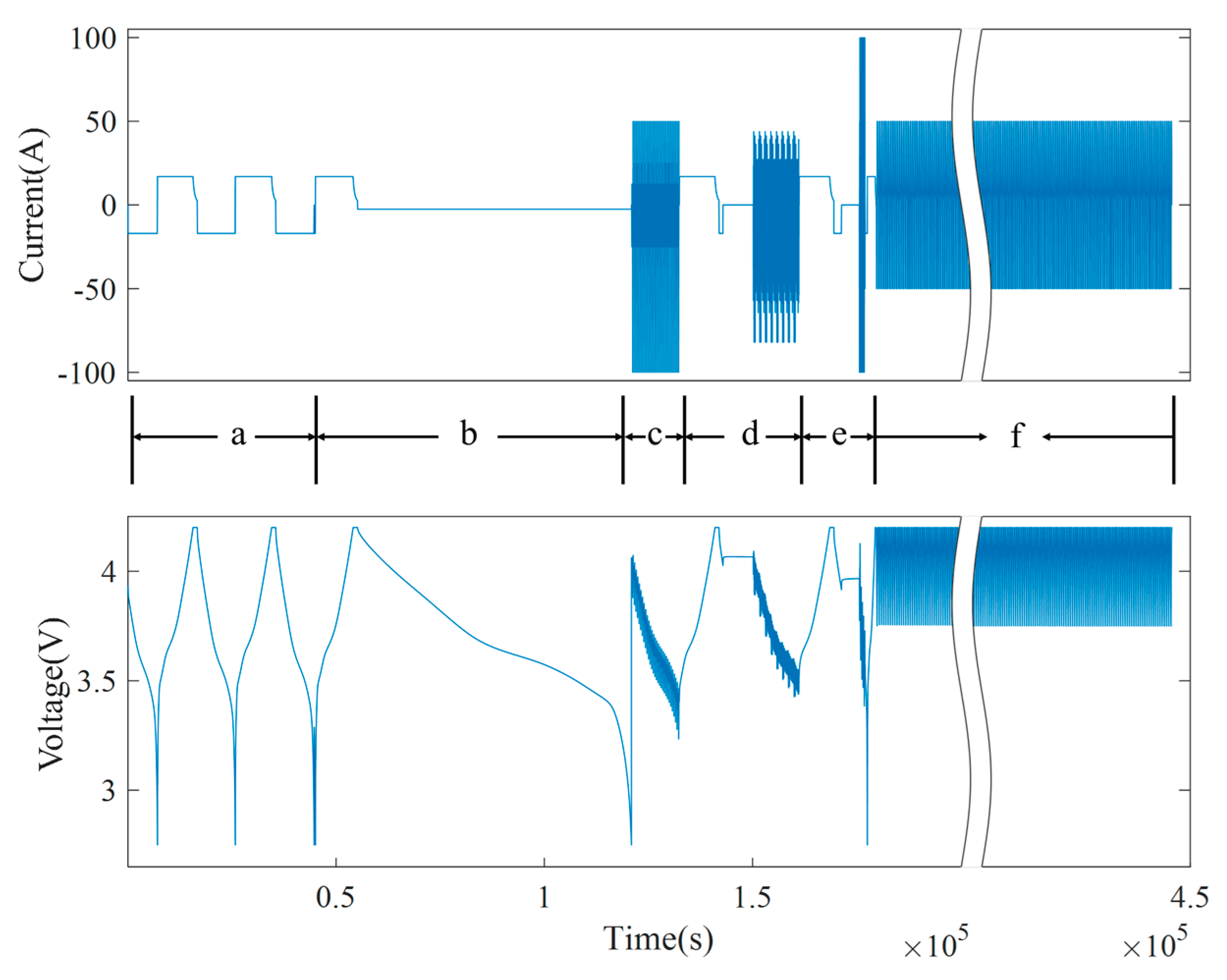
Figure 14.
Aging curves of all tested cells.
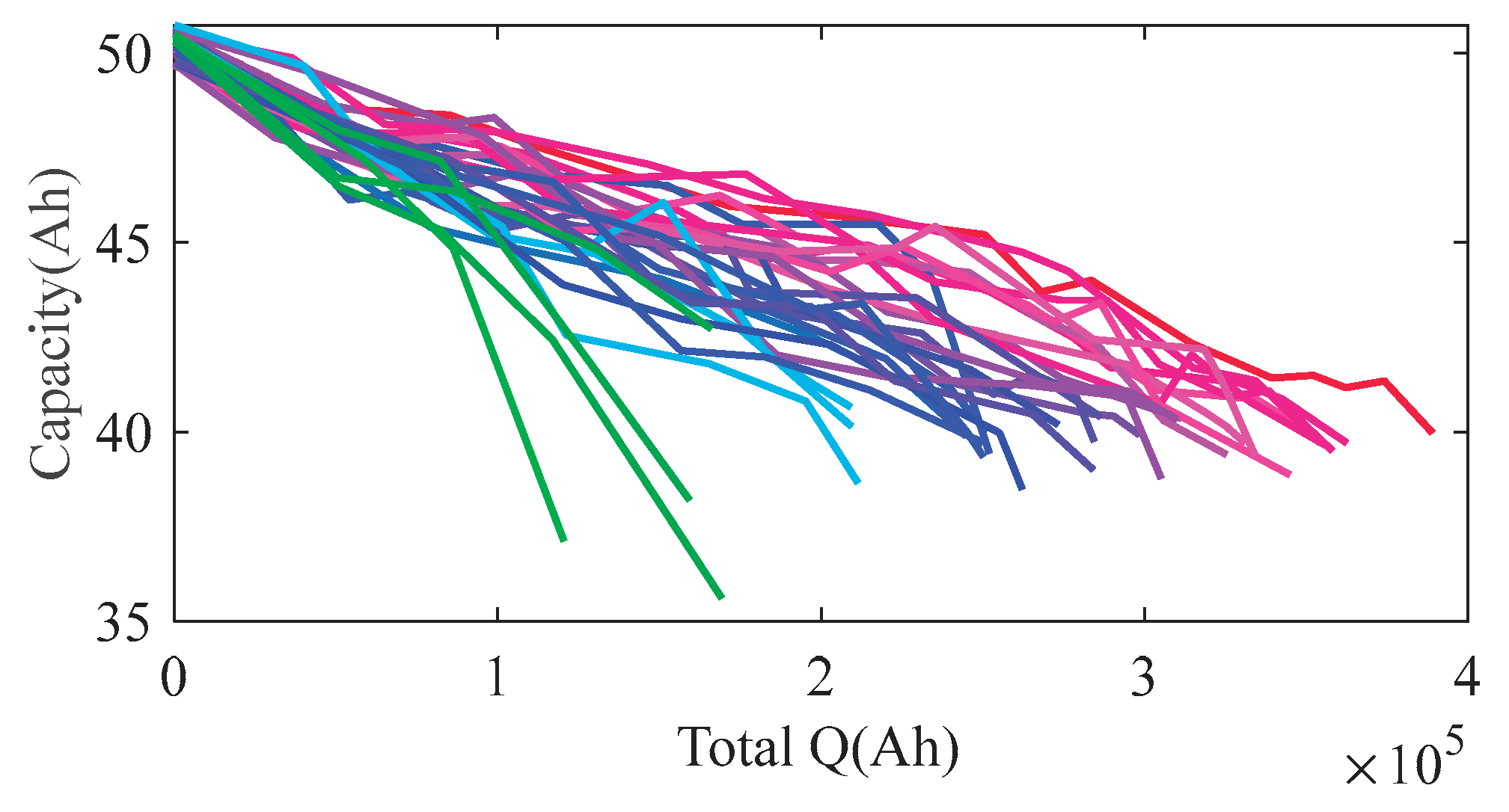
Figure 15.
Aging curves of all cells with polynomial fitting.
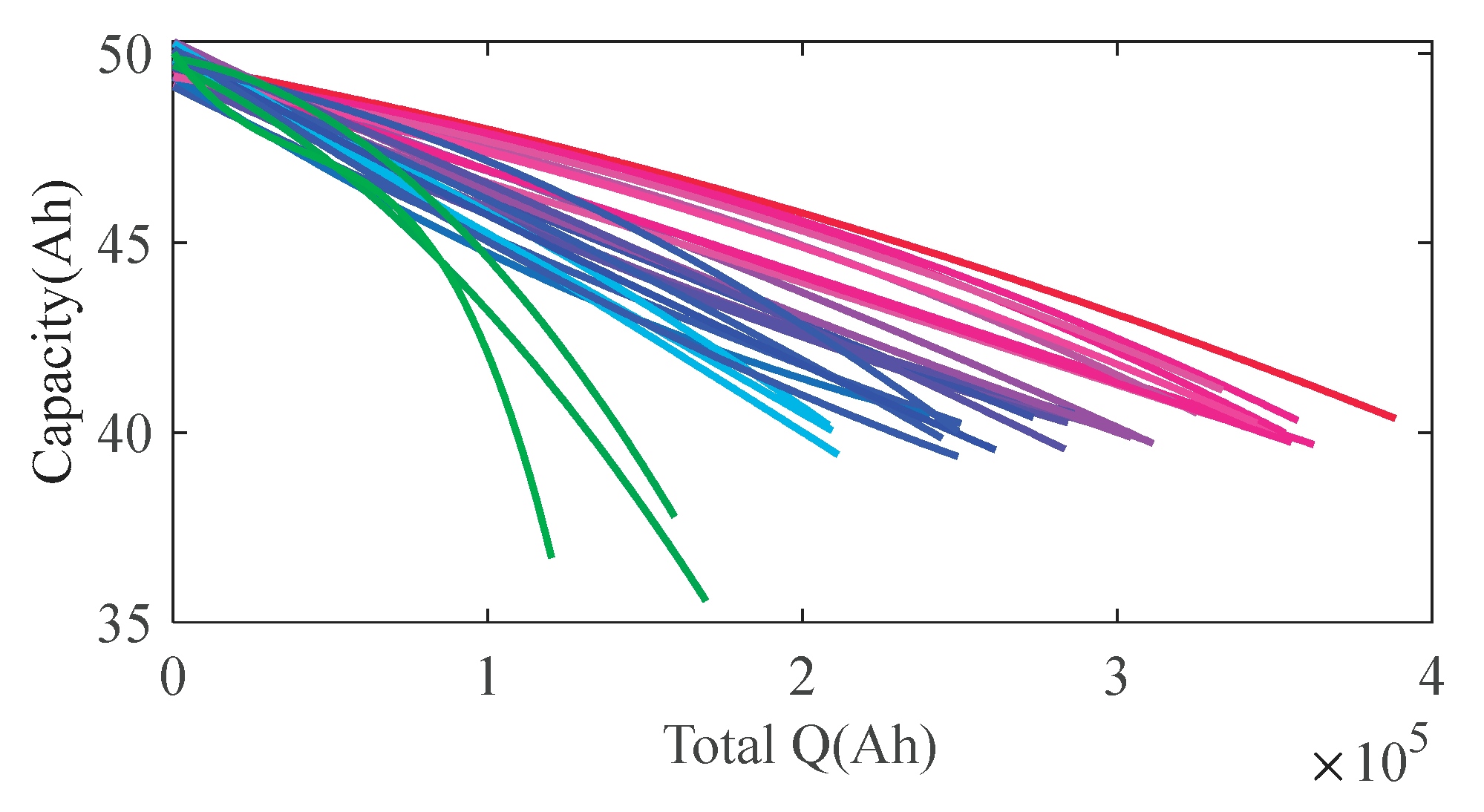
Figure 16.
Capacity-related features of all cells vs. accumulated Ah.
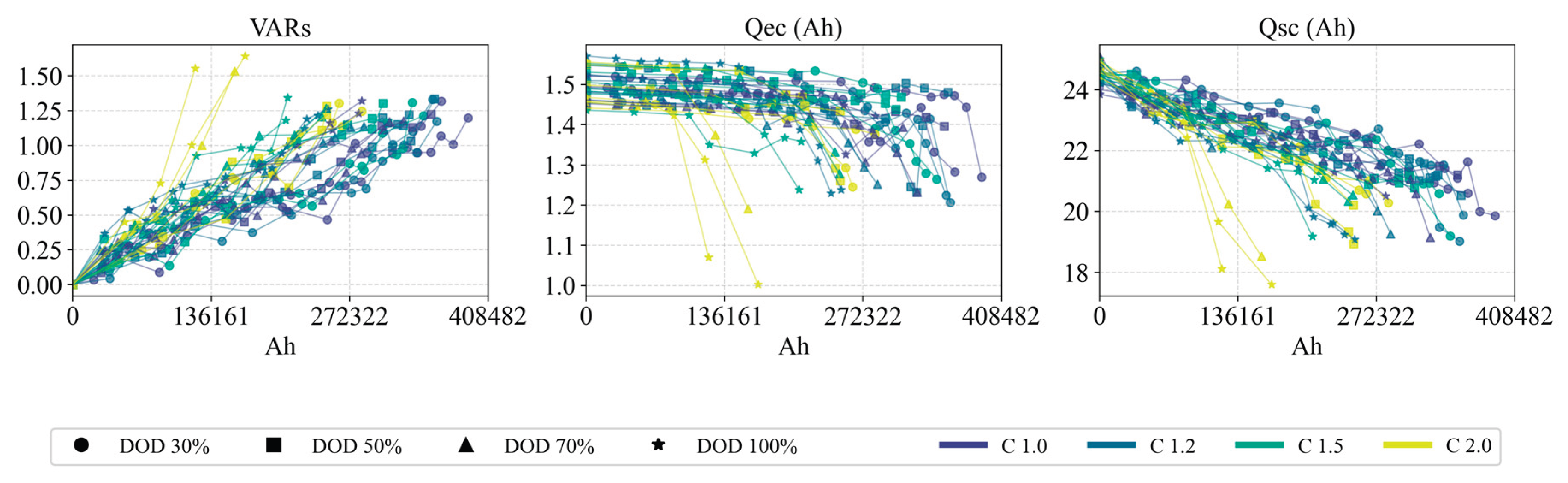
Figure 17.
Capacity-related features of all cells vs. SOH.
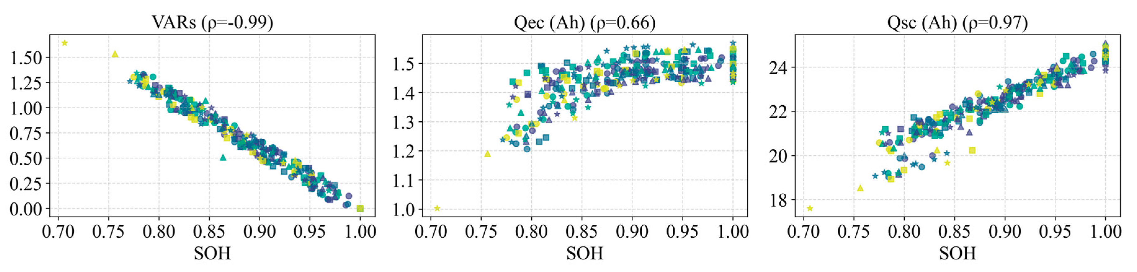
Figure 18.
Slopes of capacity features vs. for all cells.
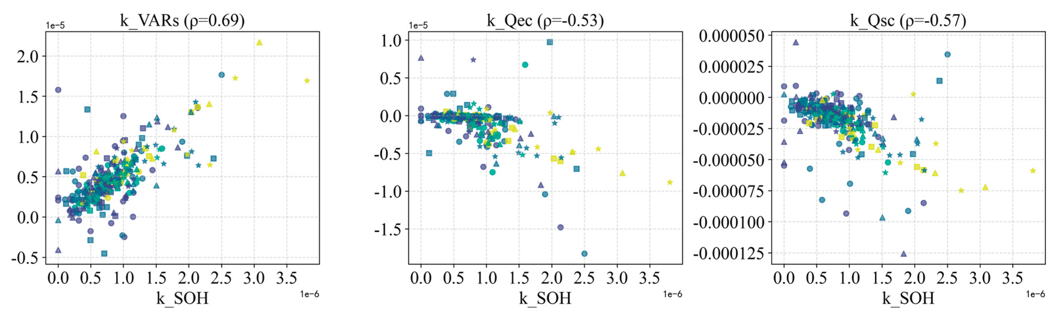
Figure 19.
IC-curve features (peak areas, heights) vs. Ah for all cells.
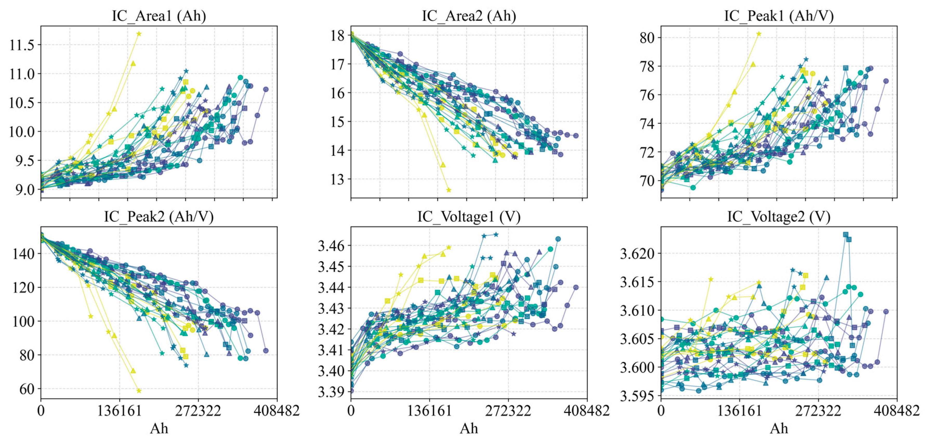
Figure 20.
IC-curve features vs. SOH for all cells.
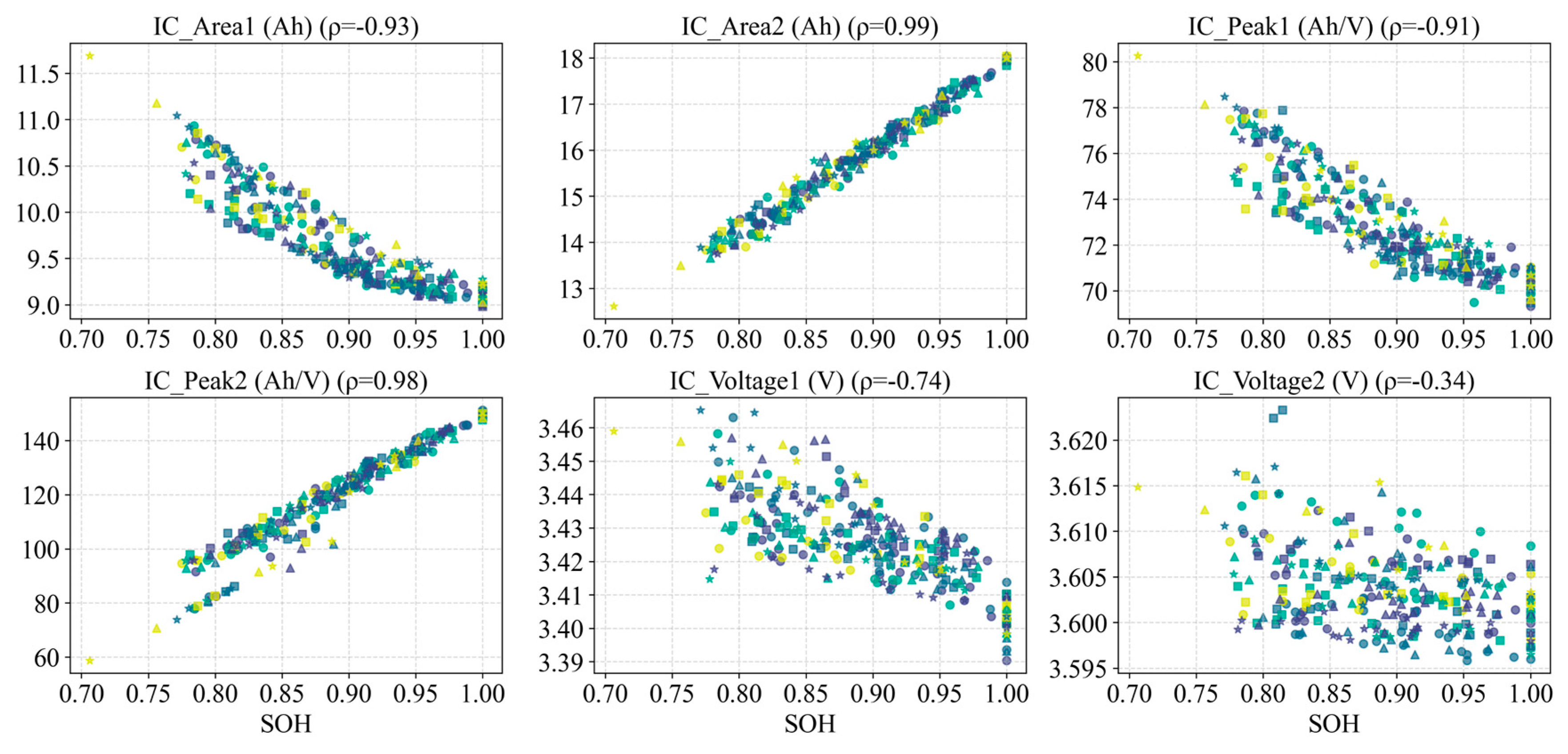
Figure 21.
Slopes of IC features vs. for all cells.
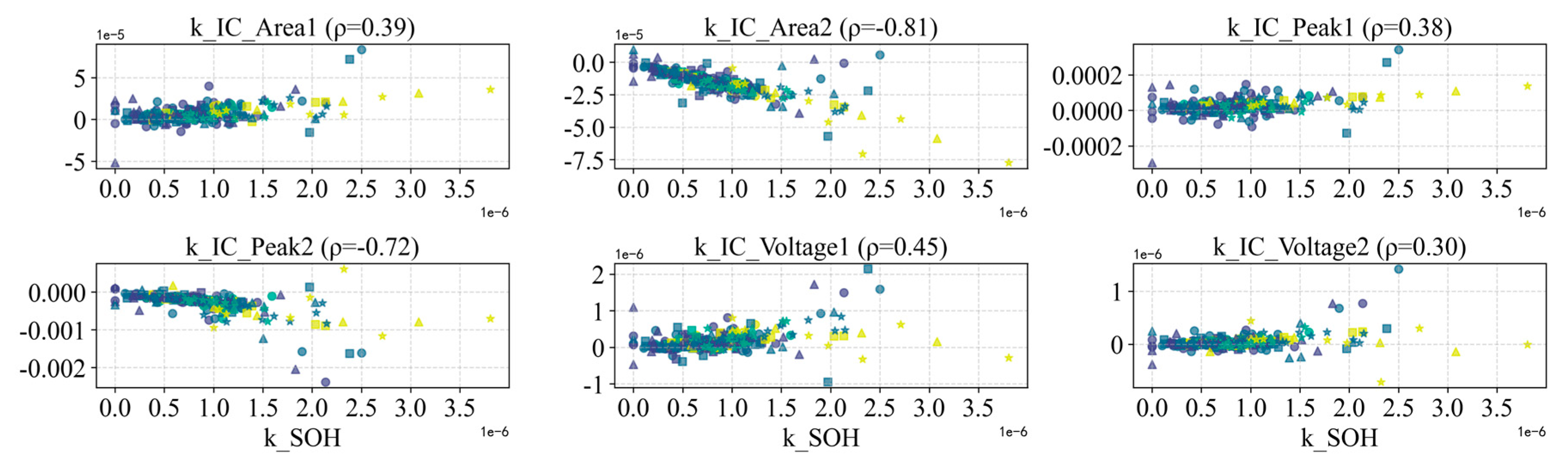
Figure 22.
Relaxation features (voltage recovery) vs. Ah for all cells.
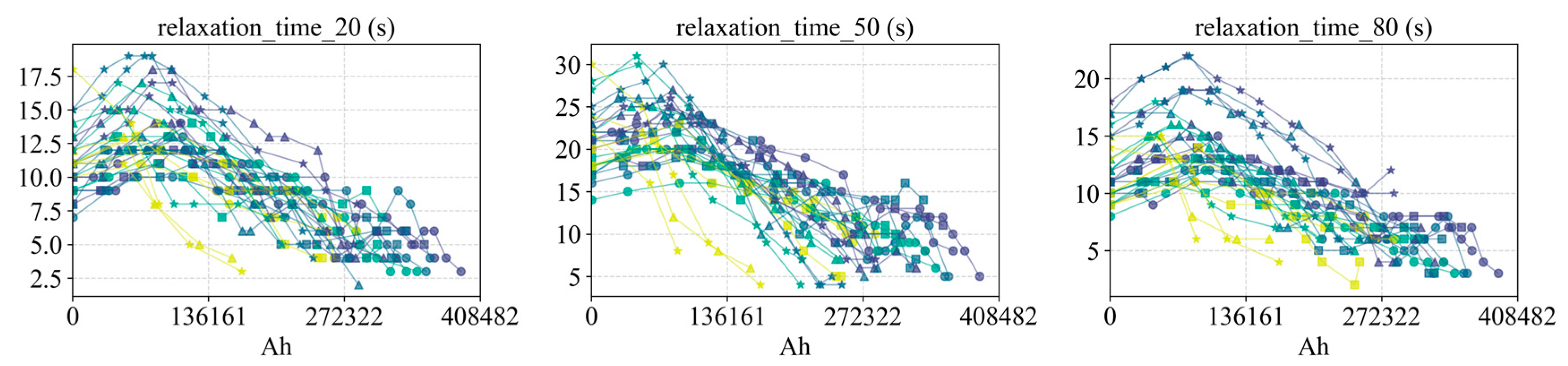
Figure 23.
Relaxation features vs. SOH for all cells.
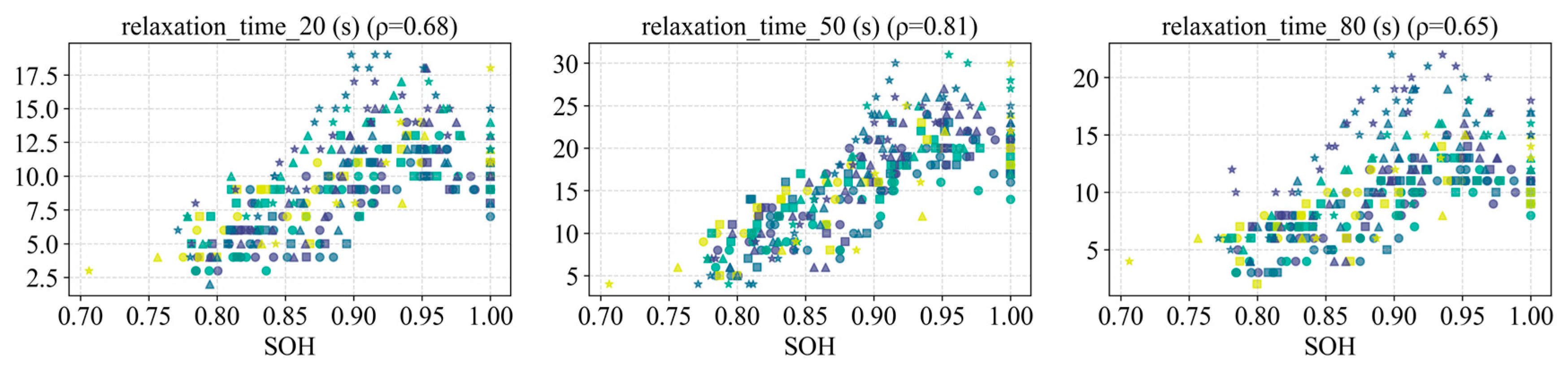
Figure 24.
Slopes of relaxation features vs. for all cells.
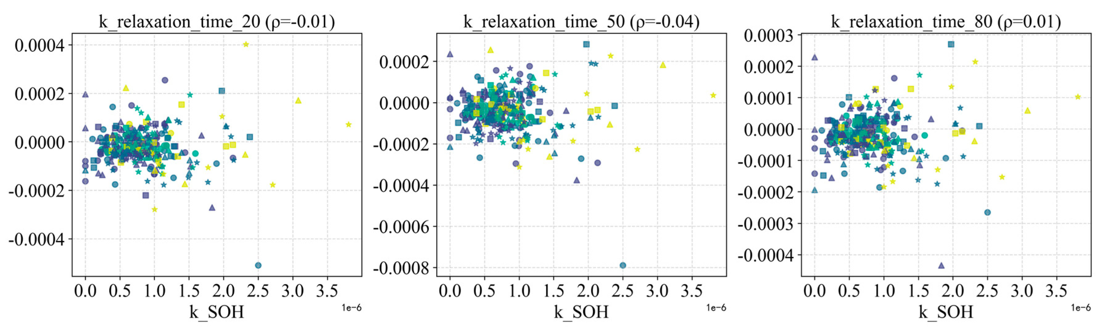
Figure 25.
Ohmic and polarization resistance vs. Ah for all cells.
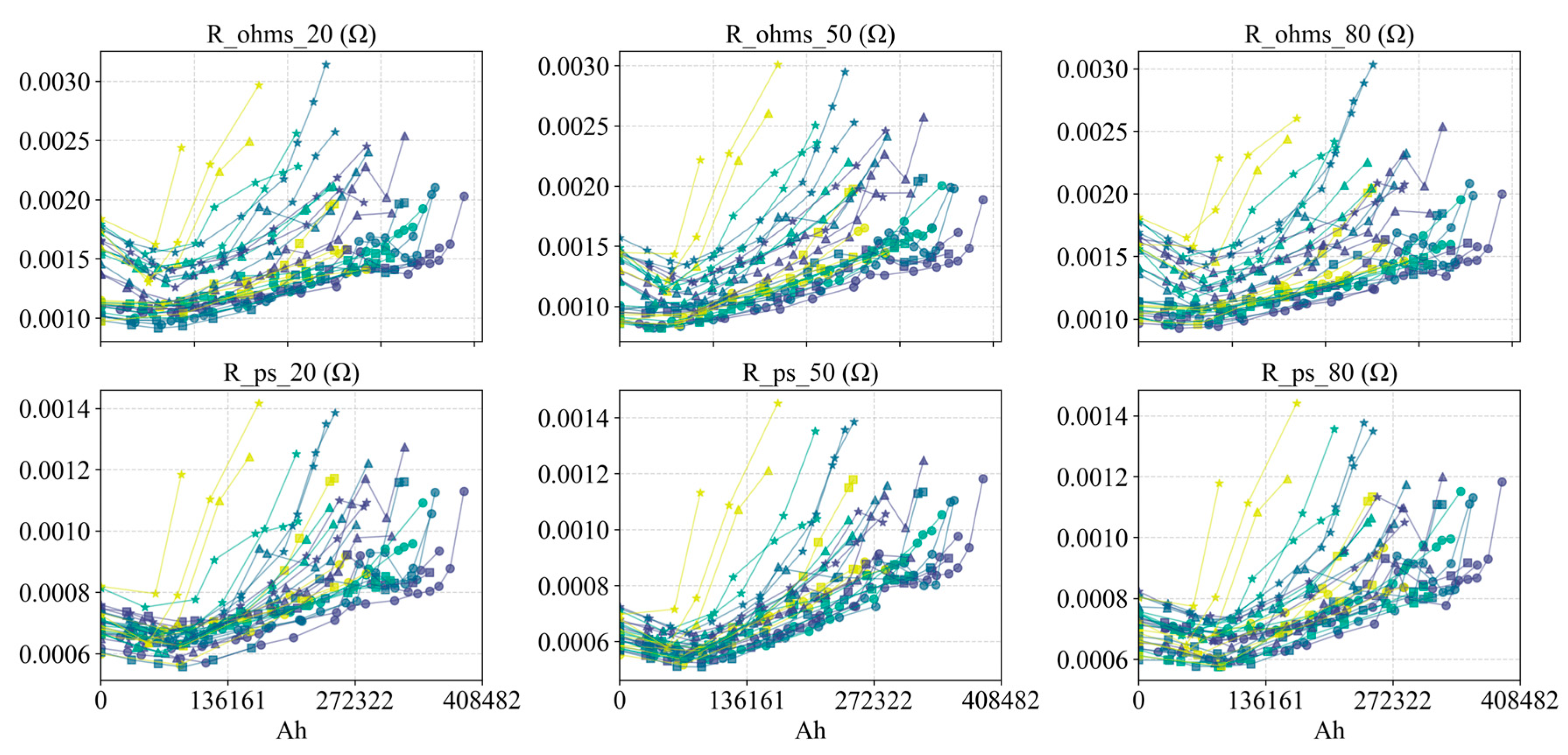
Figure 26.
Ohmic and polarization resistance vs. SOH for all cells.
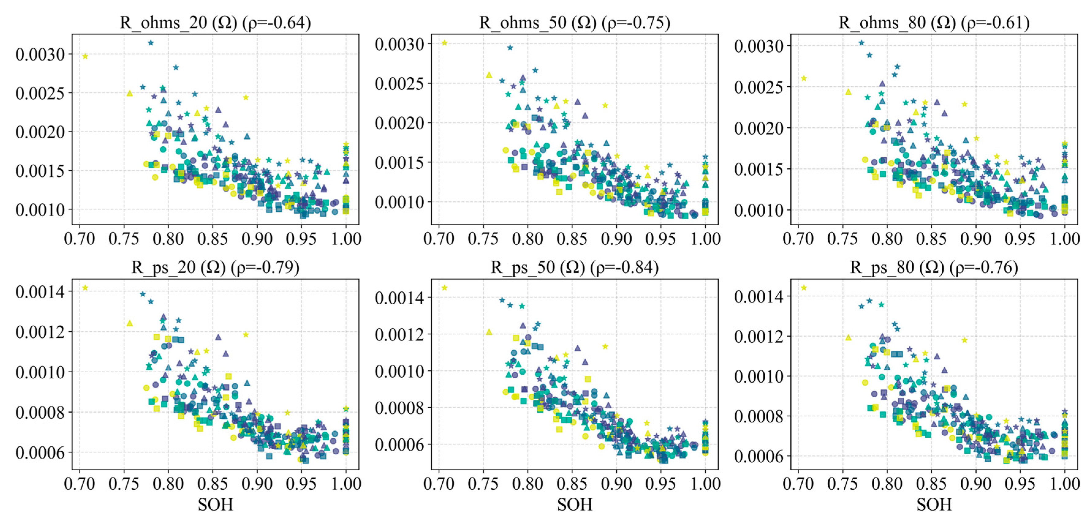
Figure 27.
Ohmic and polarization resistance slopes vs. .
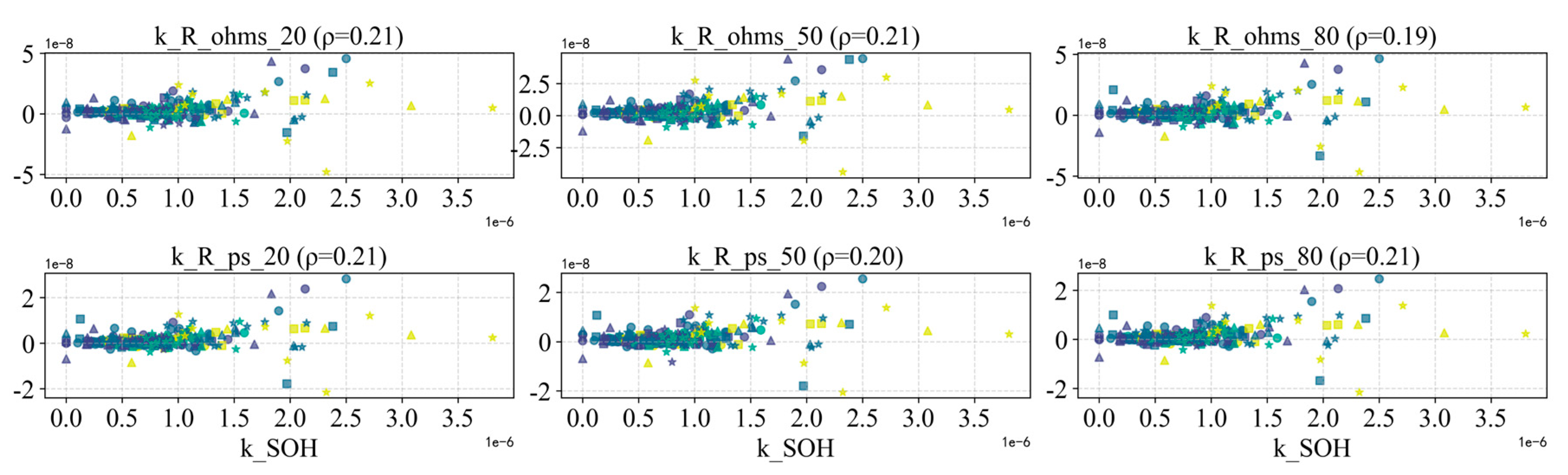
Figure 28.
Ohmic resistance vs. Ah at various SOCs (20%, 40%, 50%, 60%, 80%).
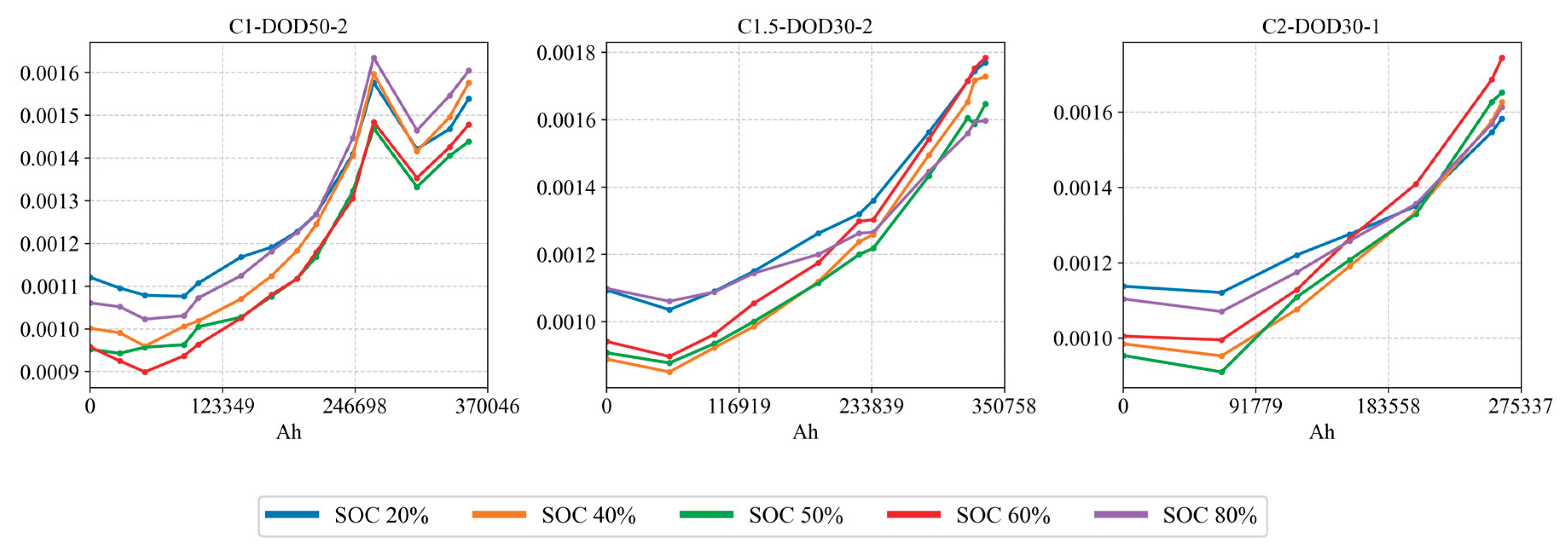
Figure 29.
Polarization resistance vs. Ah at various SOCs.
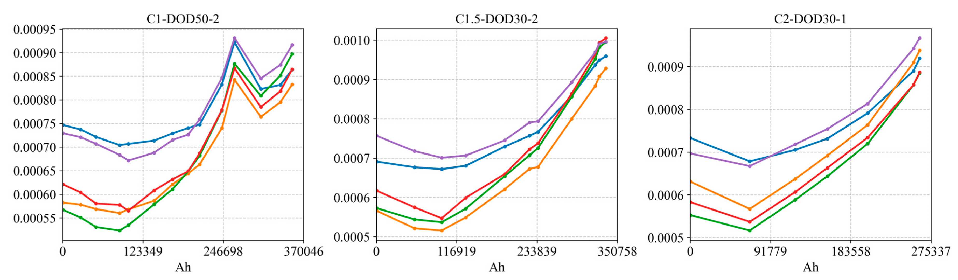
Figure 30.
DCR vs. Ah at various SOCs.
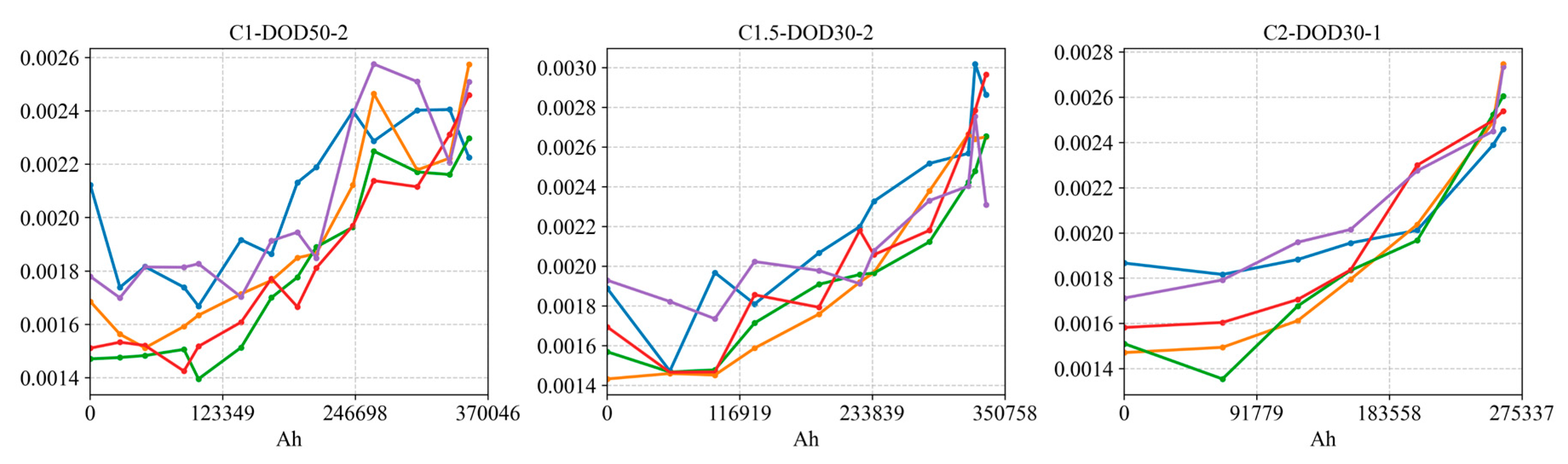
Figure 31.
DCR at 80% SOC: capacity-test measurement (purple) vs. operating condition estimate (yellow).
Figure 31.
DCR at 80% SOC: capacity-test measurement (purple) vs. operating condition estimate (yellow).
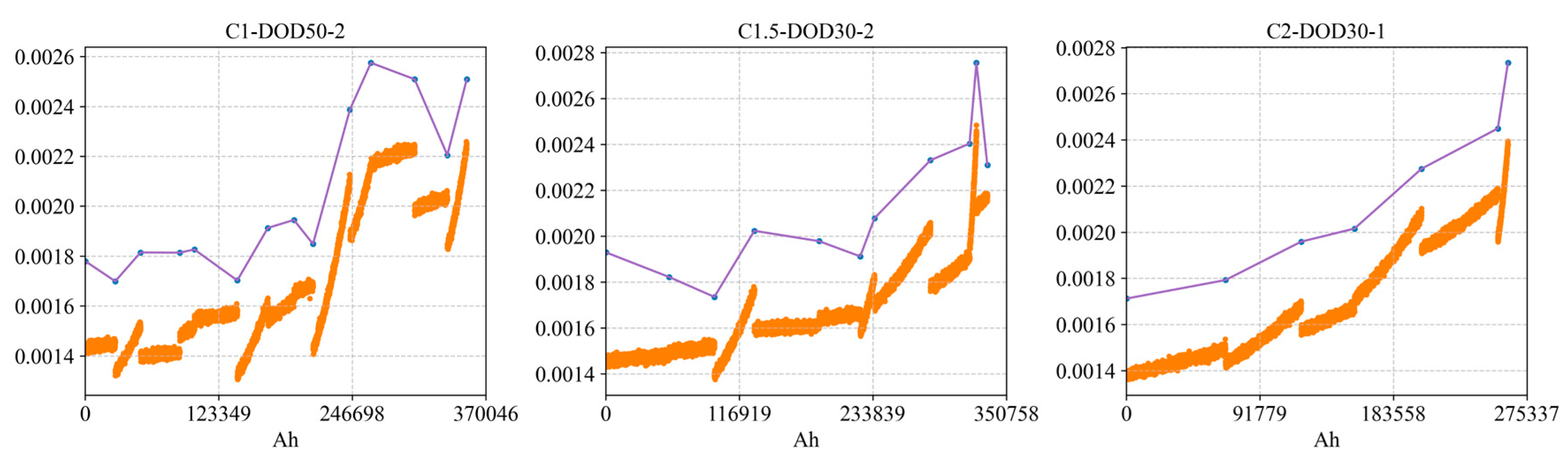
Figure 32.
Cumulative correlation ratio trends for all data (global breakpoints A = 0.90, B = 0.82).
Figure 32.
Cumulative correlation ratio trends for all data (global breakpoints A = 0.90, B = 0.82).
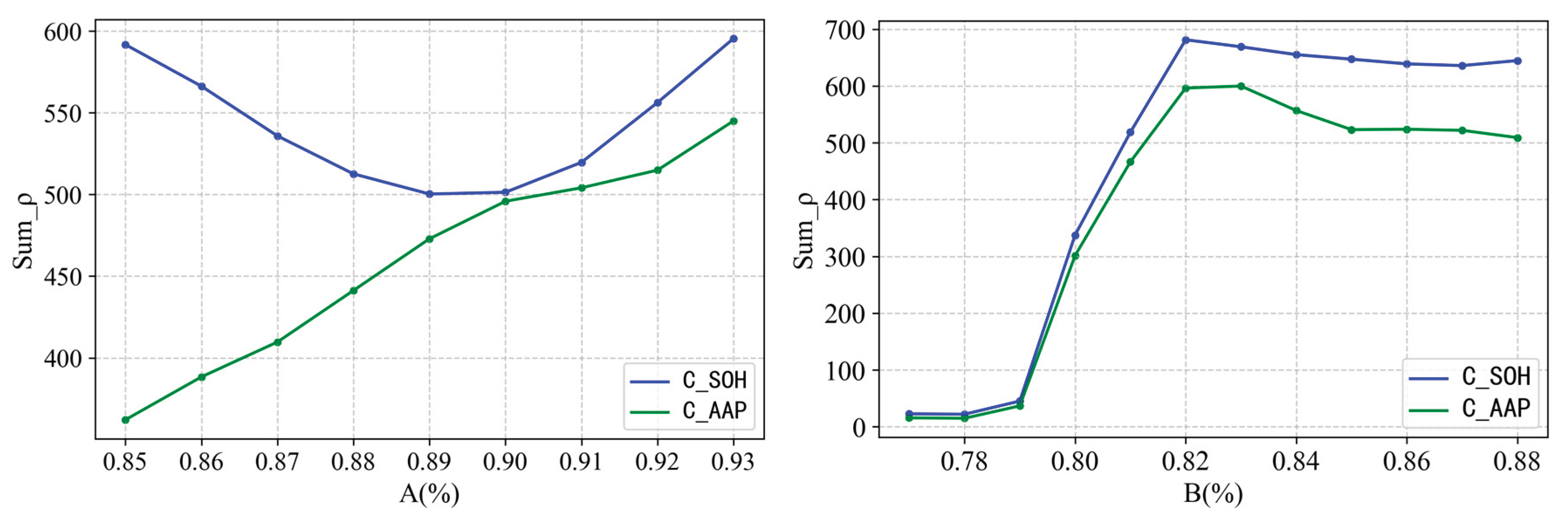
Figure 33.
SOH estimation and feature importance for test cell using Model 3 (early stage).
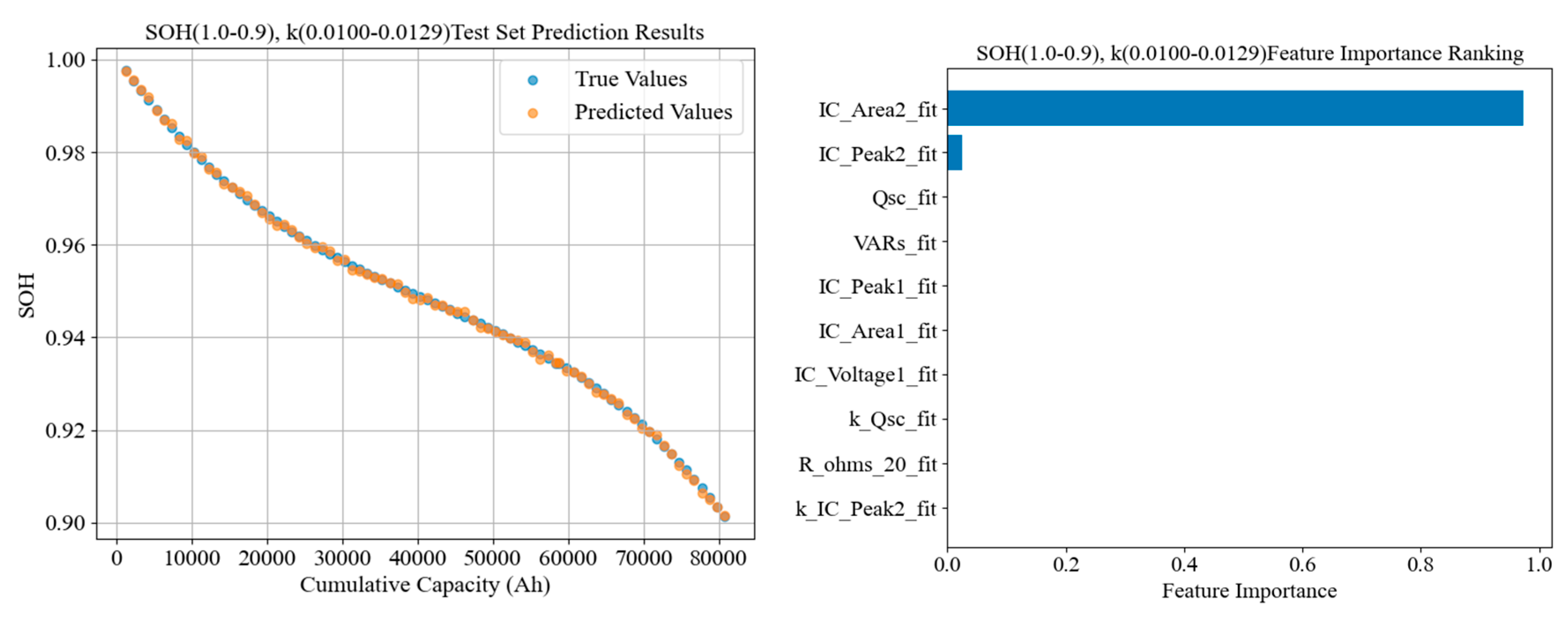
Figure 34.
SOH estimation and feature importance for test cell using Model 5 (middle stage).
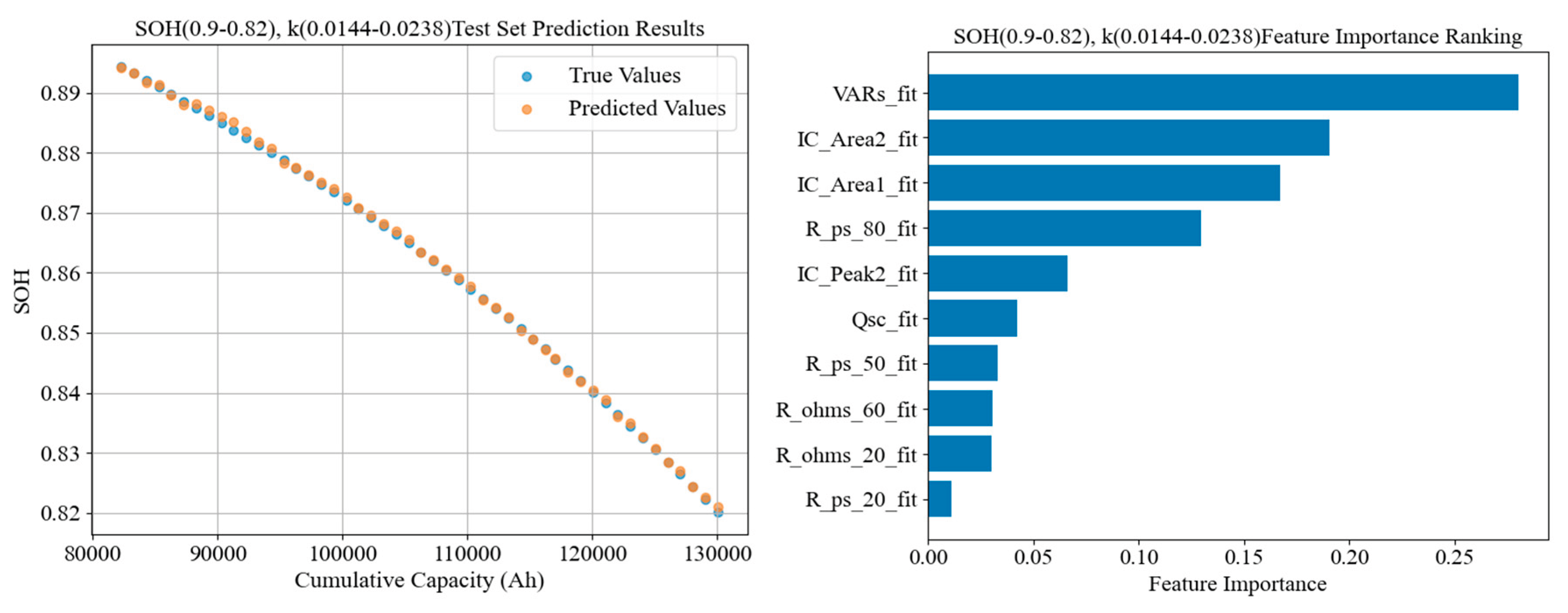
Figure 35.
SOH estimation and feature importance for test cell using Model 8 (late stage).
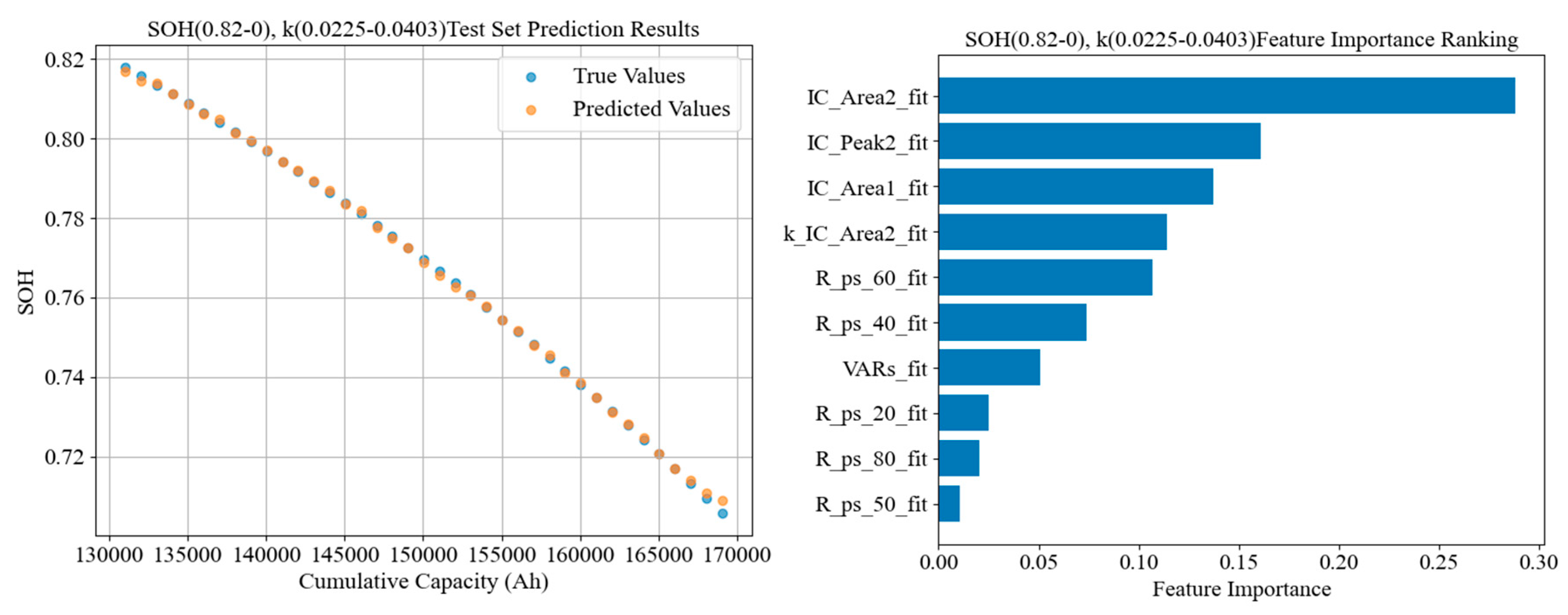
Figure 36.
Online SOH prediction and accelerated-aging warning for cell C2-DOD50-2.
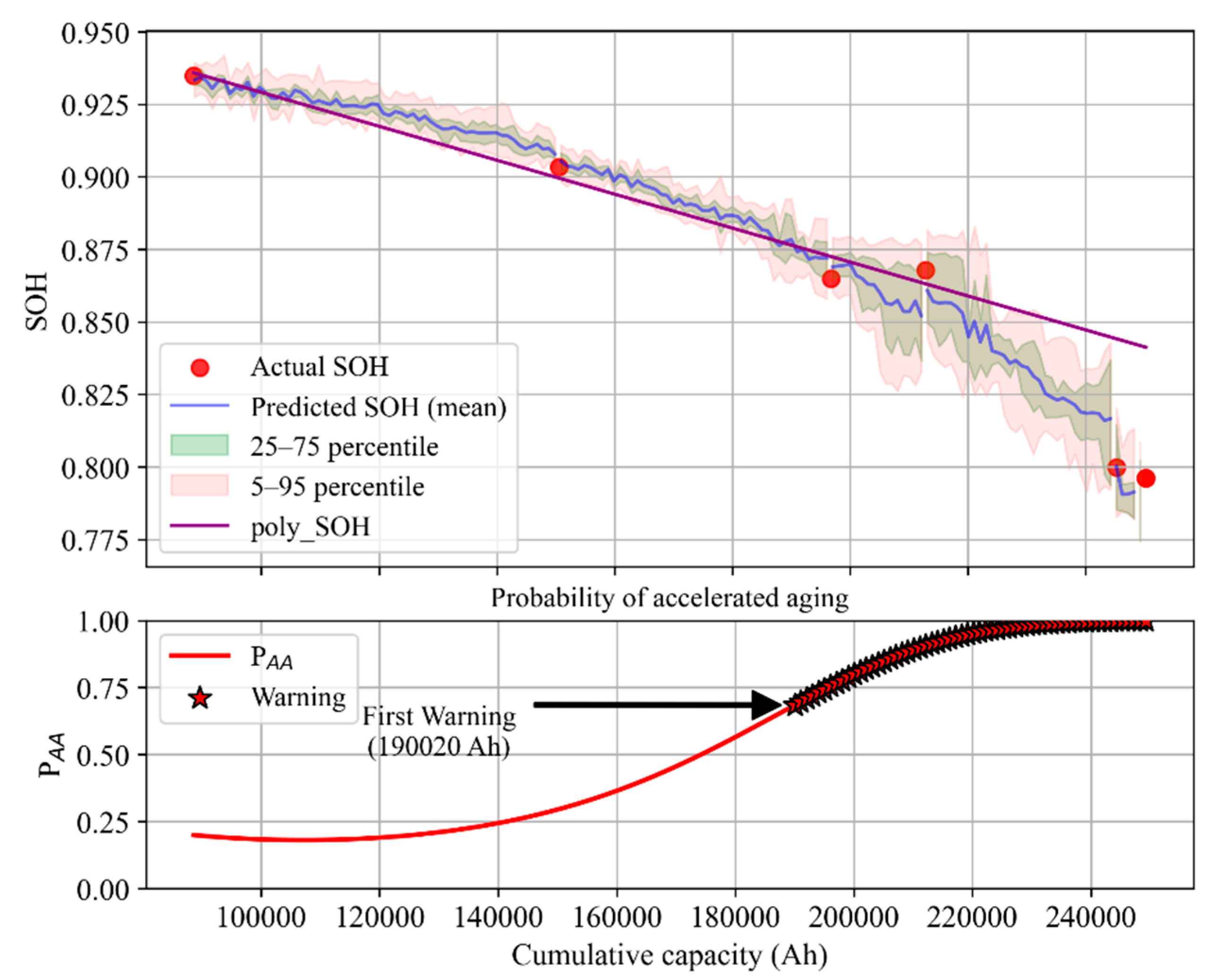
Figure 37.
Online SOH prediction and accelerated-aging warning for cell C1-DOD70-1.
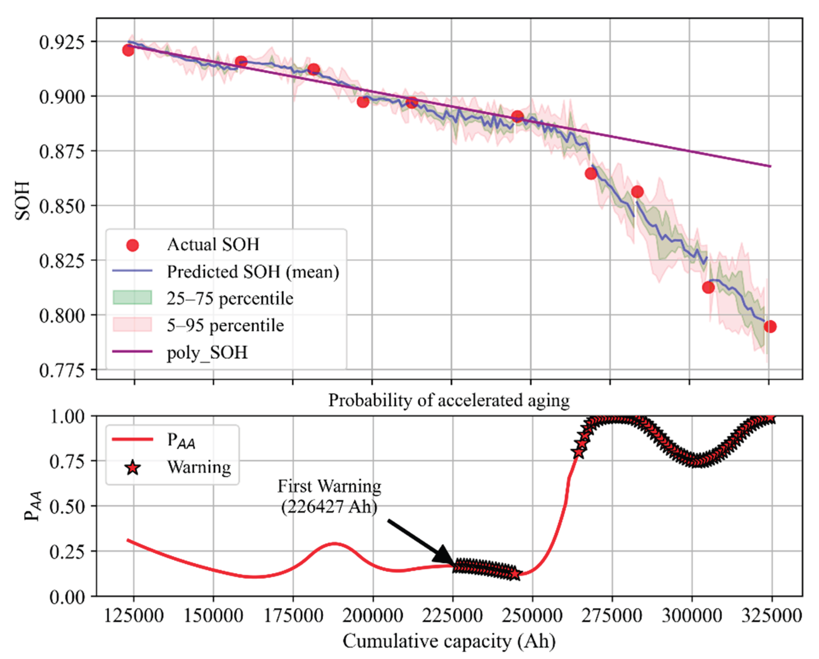
Figure 38.
Online SOH prediction and accelerated-aging warning for cell C1.2-DOD30-1.
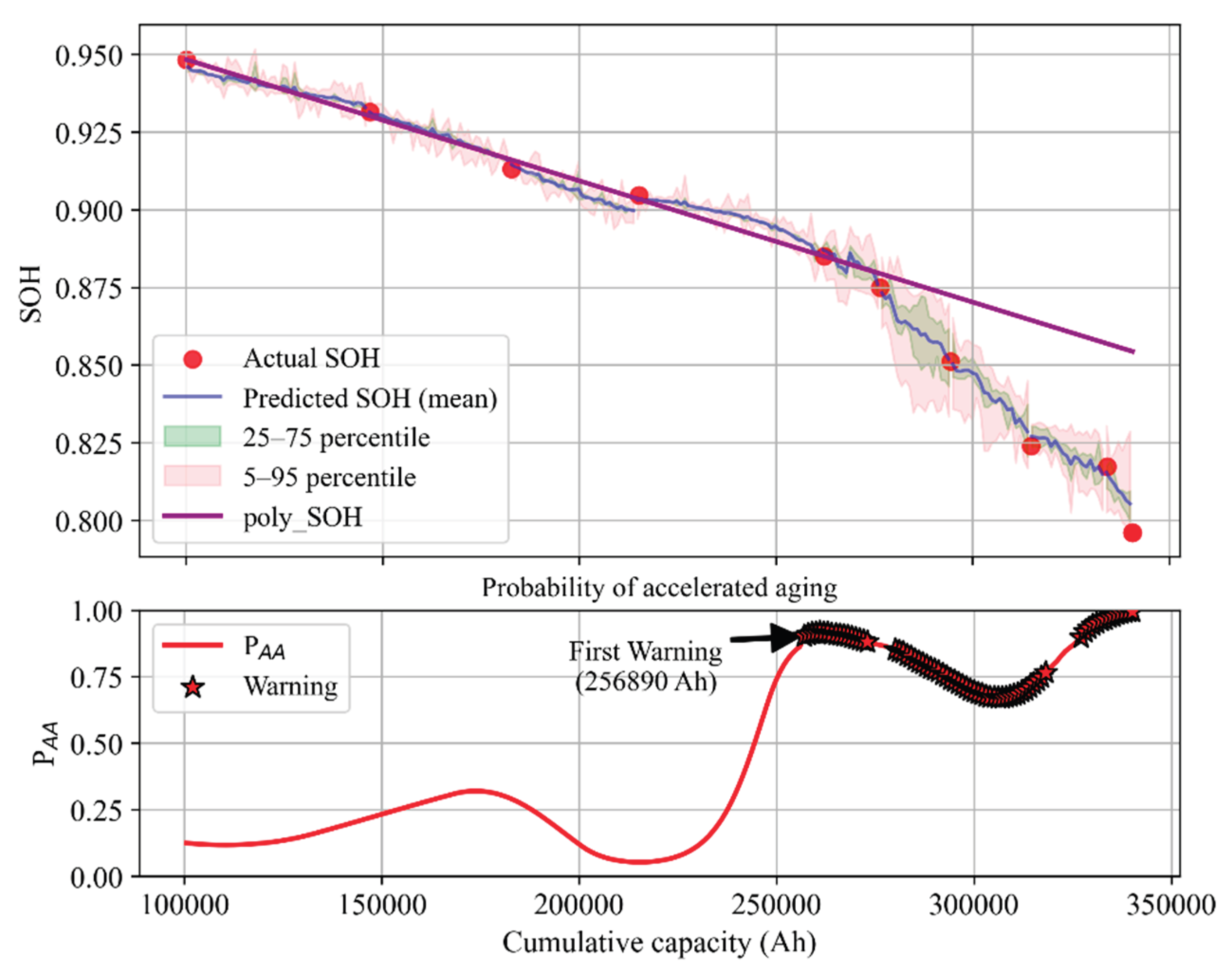
Figure 39.
Online SOH prediction and accelerated-aging warning for cell C2-DOD50-2 with injected data errors (5% missing data).
Figure 39.
Online SOH prediction and accelerated-aging warning for cell C2-DOD50-2 with injected data errors (5% missing data).
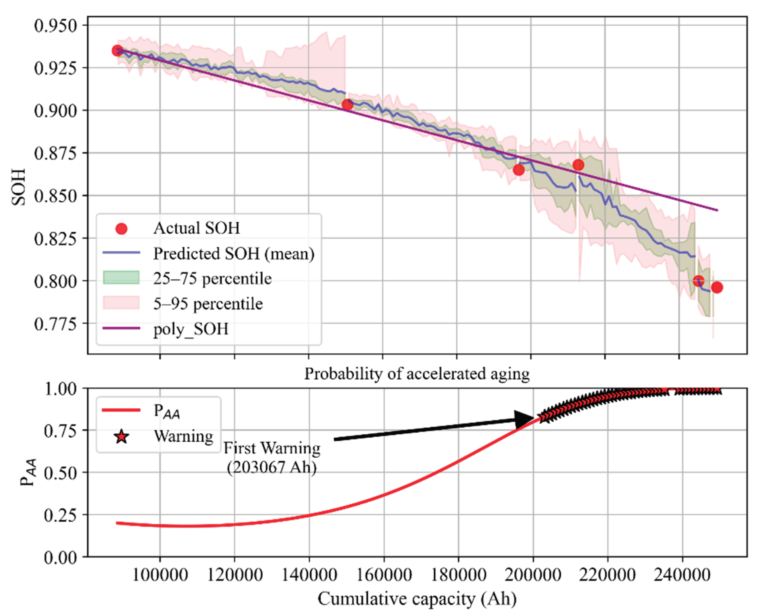
Table 1.
Typical health features corresponding to different aging stages.
| Feature | Req. cond.? | Comp. cost | Slow aging | Accelerated | Thermal |
|---|---|---|---|---|---|
| Maximum available Li-ion concentration | Yes | High | ✓ | ✓ | |
| SEI film resistance [20] | Yes | High | ✓ | ✓ | |
| Overpotential (η) | Yes | High | ✓ | ✓ | |
| Electrolyte loss | Yes | High | ✓ | ✓ | |
| Active material loss | No | Medium | ✓ | ✓ | ✓ |
| IC curve features | Yes | Medium | ✓ | ✓ | |
| Relaxation performance features | No | Medium | ✓ | ✓ | ✓ |
| Capacity variance (VAR) [21] | No | Low | ✓ | ✓ | |
| Voltage segment capacities (Qsc,Qec) [22] | No | Low | ✓ | ✓ | |
| HPPC-derived ohmic & polarization R | Yes | Low | ✓ | ✓ | ✓ |
| Pulse-derived equivalent resistance | No | Low | ✓ | ✓ | ✓ |
| Statistical metrics from CCCV curves | Yes | Low | ✓ | ✓ |
Table 2.
Aging test matrix.
| C | 1 | 1.2 | 1.5 | 2 | |
|---|---|---|---|---|---|
| DOD | |||||
| 30 | 1,2 | 9,10 | 17,18 | 25,26 | |
| 50 | 3,4 | 11,12 | 19,20 | 27,28 | |
| 70 | 5,6 | 13,14 | 21,22 | 29,30 | |
| 100 | 7,8 | 15,16 | 23,24 | 31,32 | |
Table 4.
Indexing of Models Corresponding to Different Aging Stages.
| SOH range | k range | Number of batteries available for training | Model number |
|---|---|---|---|
| 1.0-0.9 | 0.0042-0.0071 | 13 | 1 |
| 0.0071-0.0100 | 11 | 2 | |
| 0.0100-0.0129 | 6 | 3 | |
| 0.9-0.82 | 0.0049-0.0144 | 27 | 4 |
| 0.0144-0.0238 | 2 | 5 | |
| 0.0238-0.0333 | 1 | 6 | |
| 0.82-0 | 0.0047-0.0225 | 27 | 7 |
| 0.0225-0.0403 | 2 | 8 | |
| 0.0403-0.0581 | 1 | 9 |
Disclaimer/Publisher’s Note: The statements, opinions and data contained in all publications are solely those of the individual author(s) and contributor(s) and not of MDPI and/or the editor(s). MDPI and/or the editor(s) disclaim responsibility for any injury to people or property resulting from any ideas, methods, instructions or products referred to in the content. |
© 2025 by the authors. Licensee MDPI, Basel, Switzerland. This article is an open access article distributed under the terms and conditions of the Creative Commons Attribution (CC BY) license (http://creativecommons.org/licenses/by/4.0/).
Copyright: This open access article is published under a Creative Commons CC BY 4.0 license, which permit the free download, distribution, and reuse, provided that the author and preprint are cited in any reuse.


