
Submitted:
24 October 2025
Posted:
30 October 2025
You are already at the latest version
Abstract
With the rapid development of large language models (LLMs), identifying efficient strategies for training such large-scale systems has become increasingly critical. Although LLMs have achieved remarkable success across diverse applications, the necessity of maintaining full dense matrices during pre-training has been questioned, giving rise to parameter-efficient sparse pre-training methods which retains parameter-efficiency in both training and inference. These methods can be further divided into connectivity sparse training and spectral sparse training, with dynamic connectivity sparse training and low-rank factorization emerging as representative approaches for the two branches. However, a unified framework that effectively combines the strengths of both has yet to be established. In this work, we observe that the cancellation effect between the sparse and low-rank branches may limit the expressivity of the model, manifesting as output conflicts when the two components are combined. To address this issue, we propose a novel scheme that integrates dynamic sparse training with low-rank training, introducing a simple yet effective alignment loss to mitigate the disagreement between the two branches and promote better collaboration. We validate this scheme by combining a representative dynamic sparse training method, CHTs, with low-rank training, resulting in a new parameter-efficient training approach termed CHTsL. The method is evaluated on LLaMA60M and LLaMA130M using the OpenWebText and C4 datasets, where only 10\%, 20\%, and 30\% of the parameters are preserved compared to dense training. Experimental results demonstrate that our proposed scheme effectively alleviates the cancellation effect and improves training stability and performance compared to the naive combination of sparse and low-rank components. Also, the new scheme enables CHTsL to consistently outperform other parameter-efficient sparse training methods under the same parameter budget, achieving performance most close to dense training.
Keywords:
dynamic sparse training
; low-rank factorization
; spectral sparse training
; efficient training
1. Introducion
Large language models (LLMs) have attracted tremendous attention due to their superior performance across a wide range of tasks. Despite their impressive capabilities, training LLMs from scratch remains extremely memory-intensive and computation-intensive [1], making it challenging to scale such models under reasonable resource constraints. This has motivated extensive research on efficient methods that reduce computational and memory costs while retaining competitive performance. One of the most direct strategies is to reduce the number of parameters. Early studies on pruning and low-rank fine-tuning [2,3,4,5,6,7,8] have shown that even after removing or compressing a large fraction of parameters, models can still preserve much of their original representational capacity. These findings suggest that parameter-efficient model manipulation is feasible, and they naturally motivate the extension from pruning or finetuning to sparse pretraining, where models are trained from scratch under constrained parameter budgets while maintaining competitive performance compared with dense training.
We divides current approaches to sparse pre-training can be broadly into two branches: connectivity sparse training and spectral sparse training, which refers to those methods utilizing low-rank factorization during pretraining.
The former branch focuses on enforcing sparsity in the connectivity of weight matrices, with dynamic connectivity sparse training emerging as a representative technique [9,10,11,12,13,14]. Dynamic connectivity sparse training maintains a sparse connectivity pattern throughout pre-training, dynamically changing the sparse connectivity and updating active weights to approximate the capacity of dense models. Recent works have shown that on multiple tasks, dynamic sparse training can approach or even surpass the performance of dense models with as little as 10% of the trainable parameters, marking a significant step forward in efficient training [13].
The second branch, spectral sparse training [15], is typically instantiated through low-rank factorization. Since the low-rank factors are updated during training, the spectral representation they induce also evolves accordingly, which makes spectral sparse training inherently dynamic. Initially proposed in the context of LLM fine-tuning [2], low-rank methods decompose weight matrices into low-dimensional components, training only the low-rank representations while freezing the full-rank backbone. These approaches drastically reduce the number of trainable parameters and leverage the pre-trained dense model’s representational power. More recent attempts have extended low-rank factorization to the pre-training stage [15,16,17,18,19]. However, these methods still require the use of full dense matrices during the forward pass, rather than maintaining the spectral sparse structure consistently from training to inference. Overcoming this limitation, successors like CoLA [20] preserve the low-rank structure throughout both training and inference, further validating the feasibility of spectral sparse training.
While previous attempt SLTrain [21] explored combining sparse and low-rank components, the design remains limited in two key aspects. First, the sparse branch in SLTrain is static, serving only as a supplementary term to spectral sparse training rather than leveraging the full potential of dynamic connectivity sparse methods. Second, SLTrain simply performs a pure summation of sparse and low-rank outputs, without any mechanism to promote effective interaction.
In this work, we take a step in this direction. We observe that naive integration of sparse and low-rank branches often suffers from a cancellation effect, where the two components produce conflicting representations that weaken expressivity and hinder convergence. To address this challenge, we propose a new scheme that integrates dynamic connectivity sparse training with low-rank training under the guidance of alignment loss, which aligns the two branches and promotes cooperative learning. Specifically, we instantiate our framework by combining the advanced dynamic sparse training method CHTs [14] with low-rank factorization, resulting in a new parameter-efficient pre-training approach, CHTsL. Extensive experiments on LLaMA-60M and LLaMA-130M [22,23] with OpenWebText and C4 show that CHTsL consistently outperforms state-of-the-art parameter-efficient sparse training baselines under the same parameter budget. Notably, with only 10%, 20%, or 30% of parameters preserved relative to dense training, CHTsL achieves performance closest to dense models, which would benefit by retaining efficiency in training, inference, and storage.
Our contributions can be summarized as follows:
First integration of connectivity sparse and spectral sparse in dynamic sparse training. We make the first attempt to genuinely integrate connectivity sparse and spectral sparse in dynamic sparse training, with dynamic connectivity and dynamic low-rank representaion. Unlike prior work such as SLTrain, where static connectivity sparsity merely served as a supplement to spectral sparsity, our approach fully leverages the complementary strengths of both paradigms.
Alignment-enhanced unified scheme. We identify the cancellation effect as a key obstacle in combining sparse and low-rank branches, where conflicting representations weaken model expressivity. To address this, we introduce the overlapping cancellation ratio (OCR) as a quantitative measure, and propose a unified integration scheme that emphasizes interaction and cooperation rather than naive branch summation. By incorporating an alignment loss, our framework explicitly mitigates conflicts, enhances collaboration, and alleviates the observed cancellation phenomenon in attention Q and K matrices.
Instantiation with CHTsL and empirical superiority. We instantiate the framework by combining advanced CHTs with low-rank factorization, yielding the proposed method CHTsL. Extensive experiments across different datasets, models, and parameter budgets demonstrate that CHTsL achieves consistently strong performance, ranking first among all parameter-efficient methods with the same parameter scale, and approaching dense model performance with significantly fewer parameters.
2. Related Work
The rapid growth of large language models (LLMs) has stimulated extensive research into improving efficiency in pre-training. Among various directions, parameter-efficient approaches have emerged as particularly promising, aiming at training models with limited number of parameters without significantly sacrificing performance. Broadly, parameter-efficient methods in the context of pre-training can be divided into two branches: connectivity sparse training, which reduces parameters by enforcing sparse connectivity patterns, and spectral sparse training, which constrains weight matrices into low-rank subspaces. Dynamic connectivity sparse training and low-rank factorization are the representative approaches for these two paradigms.
2.1. Dynamic Connectivity Sparse Training
Connectivity sparsity originates from the classical line of pruning [24,25,26], where removing parameters from dense models was shown to preserve much of the model’s performance. Inspired by this, researchers began to explore whether sparsity could be maintained throughout training, rather than applied only as a post-hoc compression. Among these efforts, methods that promote sparse training through dynamic adjustment of connectivity have gained increasing attention, as they often outperform static sparse training approaches that prune connections solely at initialization [27,28,29,30]. The pioneering work Sparse Evolutionary Training (SET) [9] removes links while introducing random rewiring of sparse connections during training to maintain model plasticity. RigL [11] further dynamically regrows connections based on gradient for more effective exploration, though it requires computing gradients of the full weight matrix during the backward pass. MEST [12] improves upon this by leveraging both weight and gradient information. CHT [13] and its successor CHTs [14] enhance dynamic sparse training using the Cannistracci-Hebbian theory [31] from network science, inspired by brain connectomes, achieving state-of-the-art performance on multiple tasks. Collectively, these studies demonstrate that dynamic sparse training can attain competitive or even superior performance compared to dense training, while using only 10% or fewer of the parameters [14].
2.2. Low-rank Factorization for Spectral Sparse Training
Complementary to connectivity sparsity, spectral sparse training leverages low-rank factorization to reduce the dimensionality of weight matrices. This idea was first popularized in the fine-tuning setting, where LoRA [2] adapts pretrained models by learning only low-rank updates rather than full weight matrices. Subsequent works [2,3,4,5,6,7,8] further demonstrate the effectiveness of low-rank fine-tuning and inspire the exploration of training from scratch with low-rank factorization. ReLoRA [16] introduces reparameterization to improve training efficiency and stability, while GaLore [17] reduces memory usage by applying low-rank projections in the gradient space during training. However, a common limitation of these approaches is that the full dense weight matrix is still required during the forward pass, providing parameter efficiency only during training but not during inference. In contrast, CoLA [20] explicitly maintains the low-rank representation throughout both training and inference, enabling reduced storage and runtime costs. In this study, we adopt CoLA [20] as the baseline under the same restriction of parameter efficiency in both forward and backward passes.
2.3. Hybrid Attempt
Beyond individual paradigms, researchers have also begun to explore combining connectivity and spectral sparsity. SLTrain [21] represents one of the earliest attempts in this direction. It augments low-rank factorization with a sparse branch, but its design exhibits several limitations. Specifically, the sparse component is static rather than dynamic, serving merely as a supplementary term to spectral sparsity instead of leveraging genuine connectivity sparse training. Moreover, SLTrain integrates the two branches via a simple summation, without introducing any collaborative mechanism to exploit their potential synergy. As a result, while SLTrain marks an important step toward hybrid parameter-efficient pre-training, it remains an immature solution, leaving room for more principled approaches.
3. Alignment-Enhanced Integration of Connectivity Sparse and Spectral Sparse
In this section, we present a unified approach for combining dynamic sparse training (connectivity sparse) with low-rank factorization (spectral sparse) under extreme sparsity. While each method alone can improve parameter-efficiency and memory-efficiency, their naive combination often leads to conflicting outputs that limit the model’s effective capacity. We address this challenge with three key steps: (i) identifying and quantifying the cancellation effect, (ii) introducing a training framework that stabilizes low-rank outputs and encourages cooperation between branches, and (iii) instantiating a method, CHTsL, that integrates connectivity sparse and spectral sparse for dynamic sparse training based on this framework.
3.1. Cancellation Effect and OCR Metric
When a sparse branch and a low-rank branch are trained together, a common phenomenon emerges: their outputs sometimes point in opposite directions. This cancellation effect means that some portion of the signal from one branch can be neutralized by the other, wasting representational power. In other words, even if each branch individually carries meaningful information, their naive sum may not fully reflect that information, effectively underutilizing the model’s capacity.
To quantify this, we define the Overlap Cancellation Ratio (OCR):
where S and L are the outputs of the sparse and low-rank branches, respectively. OCR measures the fraction of overlapping signal that is canceled due to opposite directions, with naturally restricted in the range [0, 1). A higher OCR indicates more severe cancellation.
3.2. Training Framework: Alignment Loss and Activation Adjustment
Alignment Loss for Cooperative Learning.
When training using two distinct components, the sparse and low-rank branches can produce conflicting signals. Intuitively, if one branch pushes a feature in one direction while the other pushes in the opposite direction, the net effect is reduced expressivity. To address this cancellation effect, we introduce an alignment loss that encourages the outputs to move in similar directions:
where B is the batch size and N is the number of elements in one sample’s output at layer l. This loss penalizes discrepancies between the sparse and low-rank outputs, reducing destructive interference and letting each branch focus on complementary aspects of representation. Each layer contributes to the total alignment loss, which is then weighted in the final objective.
Activation Adjustment for Low-rank Stability.
Low-rank factorization reduces the number of trainable parameters but can sometimes produce unstable outputs, particularly under extreme sparsity. Inspired by CoLA [20], we apply a mild non-linear activation between the factorized matrices:
where is a non-linear function (SiLU [32] in our experiments). Here, the activation primarily serves to stabilize the low-rank outputs, maintaining a reasonable scale and preventing numerical issues during training. Its role is mainly supportive, ensuring the low-rank branch contributes reliably alongside the sparse branch.
Overall Objective.
Combining these ideas, the output of each and the total training loss are respectively:
where balances the contribution of alignment. This objective ensures that the sparse and low-rank branches are jointly optimized, stabilizing low-rank training and encouraging the two branches to cooperate, mitigating cancellation.
3.3. CHTsL: Instantiating the Framework
Based on this training framework, we propose CHTsL, which integrates dynamic connectivity sparse training method CHTs [14] with spectral sparse (low-rank) components. In CHTsL, the sparse branch follows the CHTs update rules, while the low-rank branch incorporates mild activation adjustment, and the alignment loss is applied layer-wise to encourage cooperative outputs. This instantiation demonstrates how our framework naturally combines dynamic connectivity and spectral sparsity, providing a practical approach for training extremely sparse models under a unified scheme. Figure 1 illustrates how CHTsL works.
4. Experiment
4.1. Models
4.2. Datasets
For training and evaluation, we adopt two widely used large-scale text corpora:
OpenWebText [33]: A publicly available open-source replication of the WebText dataset used in GPT-2. It is constructed by scraping URLs shared on Reddit with high karma scores, covering a broad range of high-quality web content.
Colossal Clean Crawled Corpus (C4) [34]: A large-scale dataset derived from web pages collected through Common Crawl. After extensive cleaning and filtering, it provides high-quality natural language text suitable for large language model pre-training.
4.3. Baseline Methods
To verify the effectiveness of our method, we compare it against several parameter-efficient training baselines with an equivalent number of trainable parameters. Specifically, we consider dynamic connectivity sparse training methods including SET [9], RigL [11], MEST [12] and CHTs [14]; spectral sparse training method CoLA [20]; hybrid method SLTrain [21]. We also report the performance of dense training for comparison.
4.4. Definition of Sparsity
Since this work integrates connectivity-based sparsity with spectral (low-rank) sparsity, it is necessary to establish a consistent definition of sparsity. For both connectivity sparse and spectral sparse (based on low-rank factorization of a full matrix), we adopt the same definition of sparsity s and corresponding density d, representing the fraction of parameters relative to a full-rank dense matrix, which allows fair comparison across methods by reflecting the total number of trainable parameters:
For a connectivity sparse method, the original sparsity corresponds to the true sparsity of the network. For a low-rank factorization of dense matrices of size with rank r, the effective sparsity is . For a method that integrates both connectivity and spectral sparsity, the total sparsity can be computed as
In our experiments, all methods are compared under the same total sparsity to ensure an equivalent number of trainable parameters. For clarity in the Section 5, we report the total sparsity of each method, and we additionally provide the sparsity-configuration for the integrated methods, which includes the sparsity s of the connectivity sparse component, the rank r of the low-rank component, and the proportion of parameters between two branches in Appendix B.
4.5. Hyperparameter Settings
Alignment-enhanced training scheme introduces the coefficient to control the effect of alignment loss. We searched the in the range [0, 0.1, 0.3 0.5, 0.7, 1] with preliminary experiments. For LLaMA-60M on OpenWebText and LLaMA-130M, the appropriate is 0.5; For LLaMA-60M on C4, the appropriate is 0.3.
For methods combining sparse and low-rank training (including SLTrain and CHTsL), the sparsity-configuration mentioned in Section 4.4 need to be considered under the same total parameter budgets. We systematically varied the allocation of parameters between the sparse and low-rank branches in steps corresponding to total sparsity of 5% and the best results across all sparsity-configurations were reported. The step size for rank adjustment in the low-rank branch was calculated based on the model architecture, resulting in approximate step values of 16 for LLaMA-60M and 24 for LLaMA-130M, of which the concrete calculation process can be found in Appendix A.
All the other hyperparameters can be found in Appendix B, which is set to be the same maximally for different methods for a fair comparison.
5. Result and Discussion
In this section, we present the experimental results. We first present the effectiveness of the alignment-enhanced training scheme by comparing it with the naive integration of CHTs and low-rank factorization. And then we compare different efficient training methods under the same parameter budget to present that CHTsL consistently improves the performance, realizing the performance most close to dense training with limited parameters.
5.1. Effectiveness of alignment-enhanced integration
Performance improvement
To verify the effictiveness of the alignment-enhanced training scheme, we compare CHTsL with the naive integration between CHTs and low-rank factorization. In Table 1, we present the result of CHTs plus low-rank with different integration strategy on different models and datasets with different total sparsity, under the constraint that sparse component and low-rank component dominates the same number of parameters (). The results are validated by Wilcoxon signed-rank test for the statistical comparison. It shows that, with , activation adjust of low-rank improves the training stability and the whole alignment training scheme makes CHTsL significantly better than the naive integration.
Eased Cancellation Effect.
Figure 2 presents the OCR defined in Equation 1, comparing the cancellation effect between the naive integration and the alignment-enhanced approach for the experiment on LLaMA-60M with the OpenWebText dataset under a total sparsity of 0.9 , with sparsity-configuration . We observe that incorporating the alignment loss significantly reduces the OCR in the Query and Key layers, with performance substantially surpassing that of the naive integration. A plausible explanation is that Q and K, as the core components of attention, directly determine the attention weights via their dot product, making them highly sensitive to inconsistencies between the dynamic sparse branch and the low-rank branch. Enforcing alignment therefore stabilizes the attention maps and mitigates gradient conflicts, whereas feed-forward or value projections are more tolerant to internal variations due to residual connections. Consequently, this targeted consistency in Q and K enhances the robustness of the attention mechanism, leading to overall performance improvements. More evidence of experiments under other sparsity levels can be found in Appendix C.
5.2. CHTsL Outperforms Other Sparse Training Methods
Table 2 reports the results of CHTsL in comparison with all baseline methods under the same total parameter budget. The results demonstrate that CHTsL consistently outperforms all other methods given the same parameter constraint. This provides strong evidence for the potential of integrating connectivity sparse training with spectral sparse training, achieving performance closest to dense training while preserving only 30% or fewer of the training parameters.
5.3. Sensitivity test for sparsity configurations
In Figure 3, we illustrate how validation perplexity (PPL↓) varies with different sparsity configurations across models and datasets under a fixed total sparsity of 0.7. On OpenWebText, when the low-rank branch dominates the parameter budget far more than the connectivity-sparse branch (sparsity in the connectivity sparse branch exceeds 0.9), performance collapses. This instability may be attributed to the dataset’s relatively limited complexity. Since OpenWebText is more homogeneous, the model becomes more sensitive to imbalanced sparsity allocation. By contrast, on C4, which contains substantially more diverse and heterogeneous text, a higher proportion of low-rank parameters proves beneficial. A possible explanation is that the increased variety of linguistic patterns likely requires broader adaptations of the entire weight matrix, making low-rank components more effective in capturing such variability.
6. Conclusions
In this work, we present a novel framework for parameter-efficient pre-training by systematically integrating connectivity sparse training with spectral sparse in dynamic sparse training. We identify the cancellation effect in naive integration as the key challenge, where conflicting representations branches reduce expressivity and hinder convergence. To address this, we introduce the overlapping cancellation ratio to quantify the effect and an alignment loss to encourage cooperative learning. Building on this framework, we instantiate CHTsL by combining the advanced dynamic sparse training method CHTs with low-rank factorization. Extensive experiments on LLaMA-60M and LLaMA-130M with OpenWebText and C4 demonstrate that CHTsL consistently outperforms existing methods under equivalent parameter budgets. Our work is the first to systematically unify dynamic connectivity and spectral sparse training, moving beyond static connectivity sparsity and naive integration; it identifies and mitigates the cancellation effect, fostering effective collaboration between the sparse and low-rank components; and it provides a practical instantiation that validates the benefits of this integration. Overall, this study offers both theoretical insights and practical solutions for efficient sparse pre-training, highlighting the potential of combining complementary sparsity paradigms to maximize model expressivity under constrained resources.
Reproducibility Statement
The code for this work is provided in the supplementary material. Detailed hyperparameter settings for each method are presented in Appendix B to facilitate reproducibility.
Appendix A Sparsity Configuration for LLaMA-60M and LLaMA-130M
The sparsity configuration for methods combining a sparse branch with a low-rank branch is defined by two values: s, the sparsity of the connectivity-sparse component, and r, the rank of the low-rank component.
In our experiments, for each fixed total sparsity, we varied the sparsity-configuration in steps of . That is, whenever the parameter count of one branch was reduced by 5% relative to dense training, the parameter count of the other branch was increased accordingly. Since the sparsity of the connectivity-sparse branch is directly tied to the total sparsity, the main challenge is determining the corresponding rank adjustment in the low-rank branch, which depends on the structure of the LLaMA model.
All linear layers in LLaMA are replaced by our sparse components. Because LLaMA models of different sizes are built from repeated Transformer blocks with identical architecture, it suffices to analyze a single block to establish the relationship between s and r. Each block contains seven linear layers, denoted as Q, K, V, O, up, down, and gate. Among them, Q, K, V, and O have weight matrices of size , while up, down, and gate have size , where h is the embedding dimension and f is the feed-forward dimension. Hence, the step size of the rank corresponding to is determined by:
For LLaMA-60M with and , this yields a rank step size of approximately . For LLaMA-130M with and , the corresponding step size is .
Appendix B Detailed Hyperparameter Settings for Each Method
For fair comparison, almost all experiments adopt the common hyperparameter settings listed in Table A1, consistent with prior work.

Table A1.
Common hyperparameter settings for experiments on LLaMA-60M and LLaMA-130M. The settings align with previous research.
Table A1.
Common hyperparameter settings for experiments on LLaMA-60M and LLaMA-130M. The settings align with previous research.
| Hyperparameter | LLaMA-60M | LLaMA-130m |
|---|---|---|
| Embedding Dimension | 512 | 768 |
| Feed-forward Dimension | 1376 | 2048 |
| Global Batch Size | 512 | 512 |
| Sequence Length | 256 | 256 |
| Training Steps | 10000 | 20000 |
| Warmup Steps | 1000 | 2000 |
| Learning Rate | 3e-3 | 3e-3 |
| Optimizer | Adam | Adam |
| Layer Number | 8 | 12 |
| Head Number | 8 | 12 |
| Iterative warmup steps | 20 | 20 |
| Update Interval for DST | 100 | 100 |
There are several exceptions, particularly for dense training and CoLA. For dense training, due to the substantially larger number of parameters, a high learning rate leads to model collapse. Therefore, we adopt a learning rate of 1e-3, following the setup in Zhang et al. [14]. For CoLA, we observed strong sensitivity to the choice of optimizer: using Adam causes training collapse (with perplexity exceeding 100). To stabilize training, we use the AdamW optimizer provided in their official code.
Method-specific hyperparameter settings are as follows:
DST methods (SET, RigL, MEST, CHTs): We follow the hyperparameter configurations reported in Zhang et al. [14]. Specifically, results for LLaMA-60M on OpenWebText are directly imported from Zhang et al. [14]. For experiments not covered in that study, we set for the BRF initialization of CHTs, as it was reported to yield the highest win rate.
CoLA: Apart from the hyperparameters in Table A1, we use the same settings as those provided in the official code release.
SLTrain: The coefficient that controls the contribution of the low-rank branch is set to 32 for LLaMA-60M and 16 for LLaMA-130M, following Han et al. [21]. We also found SLTrain to be highly sensitive to the sparsity-configuration (i.e., the allocation of parameters between branches) under total sparsities of . To provide reliable results and fair comparison, we searched configurations with a step size of 0.05 sparsity (corresponding to rank steps of 16 for LLaMA-60M and 24 for LLaMA-130M). The best configurations are summarized in Table A2.
Table A2.
The best sparsity-configuration for SLTrain under different total sparsity. refers to total sparsity, s refers to sparsity in the connectivity sparse branch, r refers to the rank in low-rank branch. The last column reports the proportion of parameters in connectivity sparse branch compared with spectral sparse (low-rank) branch.
| Dataset | Model | Sparsity-Configuration | |||
|---|---|---|---|---|---|
| s | r | ||||
| OpenWebText | LLaMA-60M | 0.9 | 0.95 | 16 | 1:1 |
| 0.8 | 0.9 | 32 | 1:1 | ||
| 0.7 | 0.85 | 48 | 1:1 | ||
| LLaMA-130M | 0.9 | 0.95 | 24 | 1:1 | |
| 0.8 | 0.85 | 24 | 3:1 | ||
| 0.7 | 0.85 | 72 | 1:1 | ||
| C4 | LLaMA-60M | 0.9 | 0.95 | 16 | 1:1 |
| 0.8 | 0.9 | 32 | 1:1 | ||
| 0.7 | 0.9 | 64 | 1:2 | ||
| LLaMA-130M | 0.9 | 0.95 | 24 | 1:1 | |
| 0.8 | 0.95 | 72 | 1:3 | ||
| 0.7 | 0.85 | 72 | 1:1 | ||
CHTsL: We employ CHTs with BRF initialization and set . The alignment loss coefficient is set to 0.5 for LLaMA-60M on OpenWebText and LLaMA-130M, and 0.3 for LLaMA-60M on C4. The sparsity-configuration is tuned with a step size of 0.05. As shown in Section 5.3, the best configurations consistently converge to 1:1 allocation between the two branches on OpenWebText, and on C4. A full summary of the best configurations is provided in Table A3.
Table A3.
The best sparsity-configuration for CHTsL under different total sparsity. refers to total sparsity, s refers to sparsity in the connectivity sparse branch, r refers to the rank in low-rank branch. The last column reports the proportion of parameters in connectivity sparse branch compared with spectral sparse (low-rank) branch.
| Dataset | Model | Sparsity-Configuration | |||
|---|---|---|---|---|---|
| s | r | ||||
| OpenWebText | LLaMA-60M | 0.9 | 0.95 | 16 | 1:1 |
| 0.8 | 0.9 | 32 | 1:1 | ||
| 0.7 | 0.85 | 48 | 1:1 | ||
| LLaMA-130M | 0.9 | 0.95 | 24 | 1:1 | |
| 0.8 | 0.9 | 48 | 1:1 | ||
| 0.7 | 0.85 | 72 | 1:1 | ||
| C4 | LLaMA-60M | 0.9 | 0.95 | 16 | 1:1 |
| 0.8 | 0.95 | 48 | 1:3 | ||
| 0.7 | 0.95 | 80 | 1:5 | ||
| LLaMA-130M | 0.9 | 0.95 | 24 | 1:1 | |
| 0.8 | 0.95 | 72 | 1:3 | ||
| 0.7 | 0.95 | 120 | 1:5 | ||
Appendix C Eased Cancellation Effect under Alignment-enhanced Integration
In this section, we present the OCR curves of different integration schemes across various total sparsity levels for LLaMA-60M on OpenWebText, as a supplement to Section 5.1. Figure A1 and Figure A2 show the OCR curves under total sparsity levels of 0.8 and 0.7, respectively, where the sparsity configuration is constrained such that the two branches contain the same number of trainable parameters. These results correspond to the second and third rows of Table 1, respectively.
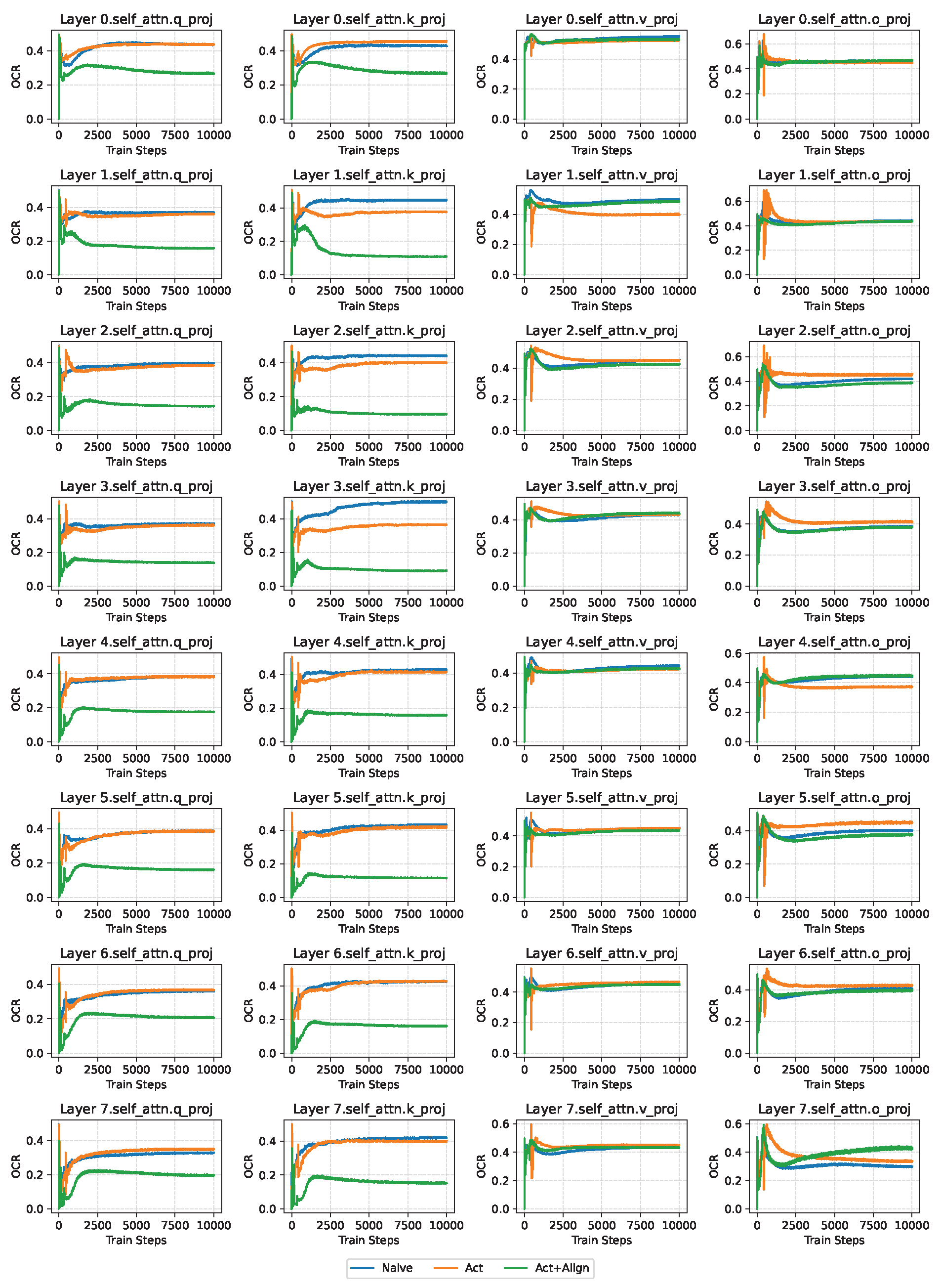
Figure A1.
The layer-wise OCR plot of LLaMA60M on OpenWebText with a total sparsity of 0.8, with sparsity-configuration . Each subplot in the figure reports the changes of OCR over training steps. The plot is based on the experiment of the second row of Table 1. For space limit, we report here the self-attention layers in the model, where each column refers to Q, K, V, O respectively.
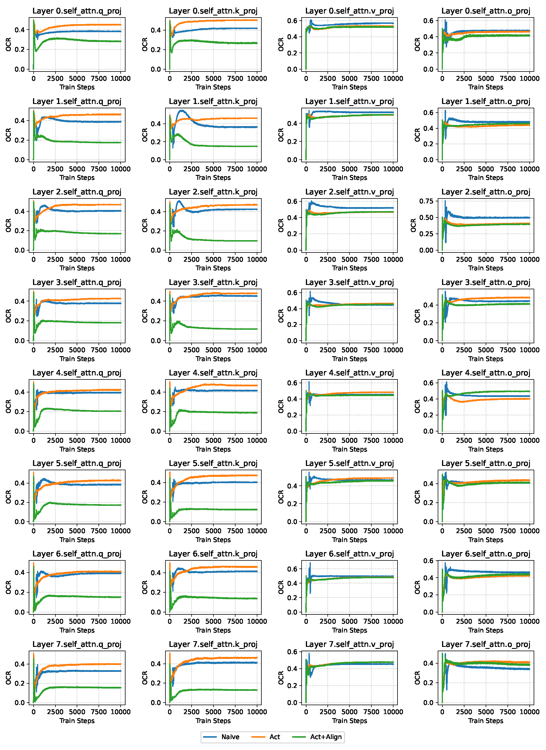
Figure A2.
The layer-wise OCR plot of LLaMA60M on OpenWebText with a total sparsity of 0.7, with sparsity-configuration . Each subplot in the figure reports the changes of OCR over training steps. The plot is based on the experiment of the third row of Table 1. For space limit, we report here the self-attention layers in the model, where each column refers to Q, K, V, O respectively.
Appendix D Usage of LLM
In this work, Large Language Model (LLM) is primarily used to assist with tasks such as text refinement, summarization, and improving the clarity and readability of the manuscript. The LLM helps streamline writing and editing, ensuring that technical content is clearly and accurately presented.
References
- Samsi, S.; Zhao, D.; McDonald, J.; Li, B.; Michaleas, A.; Jones, M.; Bergeron, W.; Kepner, J.; Tiwari, D.; Gadepally, V. From words to watts: Benchmarking the energy costs of large language model inference. In Proceedings of the 2023 IEEE High Performance Extreme Computing Conference (HPEC); IEEE, 2023; pp. 1–9. [Google Scholar]
- Hu, E.J.; Shen, Y.; Wallis, P.; Allen-Zhu, Z.; Li, Y.; Wang, S.; Wang, L.; Chen, W.; et al. Lora: Low-rank adaptation of large language models. ICLR 2022, 1, 3. [Google Scholar]
- Zhang, Q.; Chen, M.; Bukharin, A.; Karampatziakis, N.; He, P.; Cheng, Y.; Chen, W.; Zhao, T. Adalora: Adaptive budget allocation for parameter-efficient fine-tuning. arXiv 2023, arXiv:2303.10512. [Google Scholar]
- Renduchintala, A.; Konuk, T.; Kuchaiev, O. Tied-lora: Enhancing parameter efficiency of lora with weight tying. arXiv 2023, arXiv:2311.09578. [Google Scholar]
- Sheng, Y.; Cao, S.; Li, D.; Hooper, C.; Lee, N.; Yang, S.; Chou, C.; Zhu, B.; Zheng, L.; Keutzer, K.; et al. S-lora: Serving thousands of concurrent lora adapters. arXiv 2023, arXiv:2311.03285. [Google Scholar]
- Liu, S.Y.; Wang, C.Y.; Yin, H.; Molchanov, P.; Wang, Y.C.F.; Cheng, K.T.; Chen, M.H. Dora: Weight-decomposed low-rank adaptation. Proceedings of the Forty-first International Conference on Machine Learning, 2024. [Google Scholar]
- Kopiczko, D.J.; Blankevoort, T.; Asano, Y.M. Vera: Vector-based random matrix adaptation. arXiv 2023, arXiv:2310.11454. [Google Scholar]
- Dettmers, T.; Pagnoni, A.; Holtzman, A.; Zettlemoyer, L. Qlora: Efficient finetuning of quantized llms. Advances in neural information processing systems 2023, 36, 10088–10115. [Google Scholar]
- Mocanu, D.C.; Mocanu, E.; Stone, P.; Nguyen, P.H.; Gibescu, M.; Liotta, A. Scalable training of artificial neural networks with adaptive sparse connectivity inspired by network science. Nature communications 2018, 9, 2383. [Google Scholar] [CrossRef] [PubMed]
- Jayakumar, S.; Pascanu, R.; Rae, J.; Osindero, S.; Elsen, E. Top-kast: Top-k always sparse training. Advances in Neural Information Processing Systems 2020, 33, 20744–20754. [Google Scholar]
- Evci, U.; Gale, T.; Menick, J.; Castro, P.S.; Elsen, E. Rigging the lottery: Making all tickets winners. In Proceedings of the International conference on machine learning. PMLR; 2020; pp. 2943–2952. [Google Scholar]
- Yuan, G.; Ma, X.; Niu, W.; Li, Z.; Kong, Z.; Liu, N.; Gong, Y.; Zhan, Z.; He, C.; Jin, Q.; et al. Mest: Accurate and fast memory-economic sparse training framework on the edge. Advances in Neural Information Processing Systems 2021, 34, 20838–20850. [Google Scholar]
- Zhang, Y.; Zhao, J.; Wu, W.; Muscoloni, A. Epitopological learning and cannistraci-hebb network shape intelligence brain-inspired theory for ultra-sparse advantage in deep learning. In Proceedings of the The Twelfth International Conference on Learning Representations; 2024. [Google Scholar]
- Zhang, Y.; Cerretti, D.; Zhao, J.; Wu, W.; Liao, Z.; Michieli, U.; Cannistraci, C.V. Brain network science modelling of sparse neural networks enables Transformers and LLMs to perform as fully connected. arXiv 2025, arXiv:2501.19107. [Google Scholar]
- Zhao, J.; Zhang, Y.; Li, X.; Liu, H.; Cannistraci, C.V. Sparse Spectral Training and Inference on Euclidean and Hyperbolic Neural Networks. arXiv 2024, arXiv:2405.15481. [Google Scholar] [CrossRef]
- Lialin, V.; Shivagunde, N.; Muckatira, S.; Rumshisky, A. Relora: High-rank training through low-rank updates. arXiv 2023, arXiv:2307.05695. [Google Scholar]
- Zhao, J.; Zhang, Z.; Chen, B.; Wang, Z.; Anandkumar, A.; Tian, Y. Galore: Memory-efficient llm training by gradient low-rank projection. arXiv 2024, arXiv:2403.03507. [Google Scholar]
- Xia, W.; Qin, C.; Hazan, E. Chain of lora: Efficient fine-tuning of language models via residual learning. arXiv 2024, arXiv:2401.04151. [Google Scholar]
- Meng, X.; Dai, D.; Luo, W.; Yang, Z.; Wu, S.; Wang, X.; Wang, P.; Dong, Q.; Chen, L.; Sui, Z. Periodiclora: Breaking the low-rank bottleneck in lora optimization. arXiv 2024, arXiv:2402.16141. [Google Scholar]
- Liu, Z.; Zhang, R.; Wang, Z.; Yang, Z.; Hovland, P.; Nicolae, B.; Cappello, F.; Zhang, Z. Cola: Compute-efficient pre-training of llms via low-rank activation. arXiv 2025, arXiv:2502.10940. [Google Scholar]
- Han, A.; Li, J.; Huang, W.; Hong, M.; Takeda, A.; Jawanpuria, P.K.; Mishra, B. SLTrain: a sparse plus low rank approach for parameter and memory efficient pretraining. Advances in Neural Information Processing Systems 2024, 37, 118267–118295. [Google Scholar]
- Touvron, H.; Lavril, T.; Izacard, G.; Martinet, X.; Lachaux, M.A.; Lacroix, T.; Rozière, B.; Goyal, N.; Hambro, E.; Azhar, F.; et al. Llama: Open and efficient foundation language models. arXiv 2023, arXiv:2302.13971. [Google Scholar] [CrossRef]
- Touvron, H.; Martin, L.; Stone, K.; Albert, P.; Almahairi, A.; Babaei, Y.; Bashlykov, N.; Batra, S.; Bhargava, P.; Bhosale, S.; et al. Llama 2: Open foundation and fine-tuned chat models. arXiv 2023, arXiv:2307.09288. [Google Scholar] [CrossRef]
- LeCun, Y.; Denker, J.; Solla, S. Optimal brain damage. Advances in neural information processing systems 1989, 2. [Google Scholar]
- Han, S.; Mao, H.; Dally, W.J. Deep compression: Compressing deep neural networks with pruning, trained quantization and huffman coding. arXiv 2015, arXiv:1510.00149. [Google Scholar]
- Molchanov, P.; Tyree, S.; Karras, T.; Aila, T.; Kautz, J. Pruning convolutional neural networks for resource efficient inference. arXiv 2016, arXiv:1611.06440. [Google Scholar]
- Prabhu, A.; Varma, G.; Namboodiri, A. Deep expander networks: Efficient deep networks from graph theory. Proceedings of the Proceedings of the European Conference on Computer Vision (ECCV), 2018; 20–35. [Google Scholar]
- Lee, N.; Ajanthan, T.; Torr, P.H. Snip: Single-shot network pruning based on connection sensitivity. arXiv 2018, arXiv:1810.02340. [Google Scholar]
- Dao, T.; Chen, B.; Sohoni, N.S.; Desai, A.; Poli, M.; Grogan, J.; Liu, A.; Rao, A.; Rudra, A.; Ré, C. Monarch: Expressive structured matrices for efficient and accurate training. In Proceedings of the International Conference on Machine Learning. PMLR; 2022; pp. 4690–4721. [Google Scholar]
- Stewart, J.; Michieli, U.; Ozay, M. Data-free model pruning at initialization via expanders. Proceedings of the Proceedings of the IEEE/CVF Conference on Computer Vision and Pattern Recognition, 2023; 4519–4524. [Google Scholar]
- Muscoloni, A.; Michieli, U.; Zhang, Y.; Cannistraci, C.V. Adaptive network automata modelling of complex networks. 2022. [Google Scholar]
- Hendrycks, D.; Gimpel, K. Gaussian error linear units (gelus). arXiv 2016, arXiv:1606.08415. [Google Scholar]
- Gokaslan, A.; Cohen, V. OpenWebText Corpus. 2019. Available online: http://Skylion007.github.io/OpenWebTextCorpus.
- Raffel, C.; Shazeer, N.; Roberts, A.; Lee, K.; Narang, S.; Matena, M.; Zhou, Y.; Li, W.; Liu, P.J. Exploring the limits of transfer learning with a unified text-to-text transformer. Journal of machine learning research 2020, 21, 1–67. [Google Scholar]
Figure 1.
Workflow of CHTsL. The figure illustrates CHTsL as an example of alignment-enhanced integration between dynamic connectivity sparse training and spectral sparse training. Specifically, the dynamic connectivity sparse branch adopts the CHTs method.
Figure 1.
Workflow of CHTsL. The figure illustrates CHTsL as an example of alignment-enhanced integration between dynamic connectivity sparse training and spectral sparse training. Specifically, the dynamic connectivity sparse branch adopts the CHTs method.
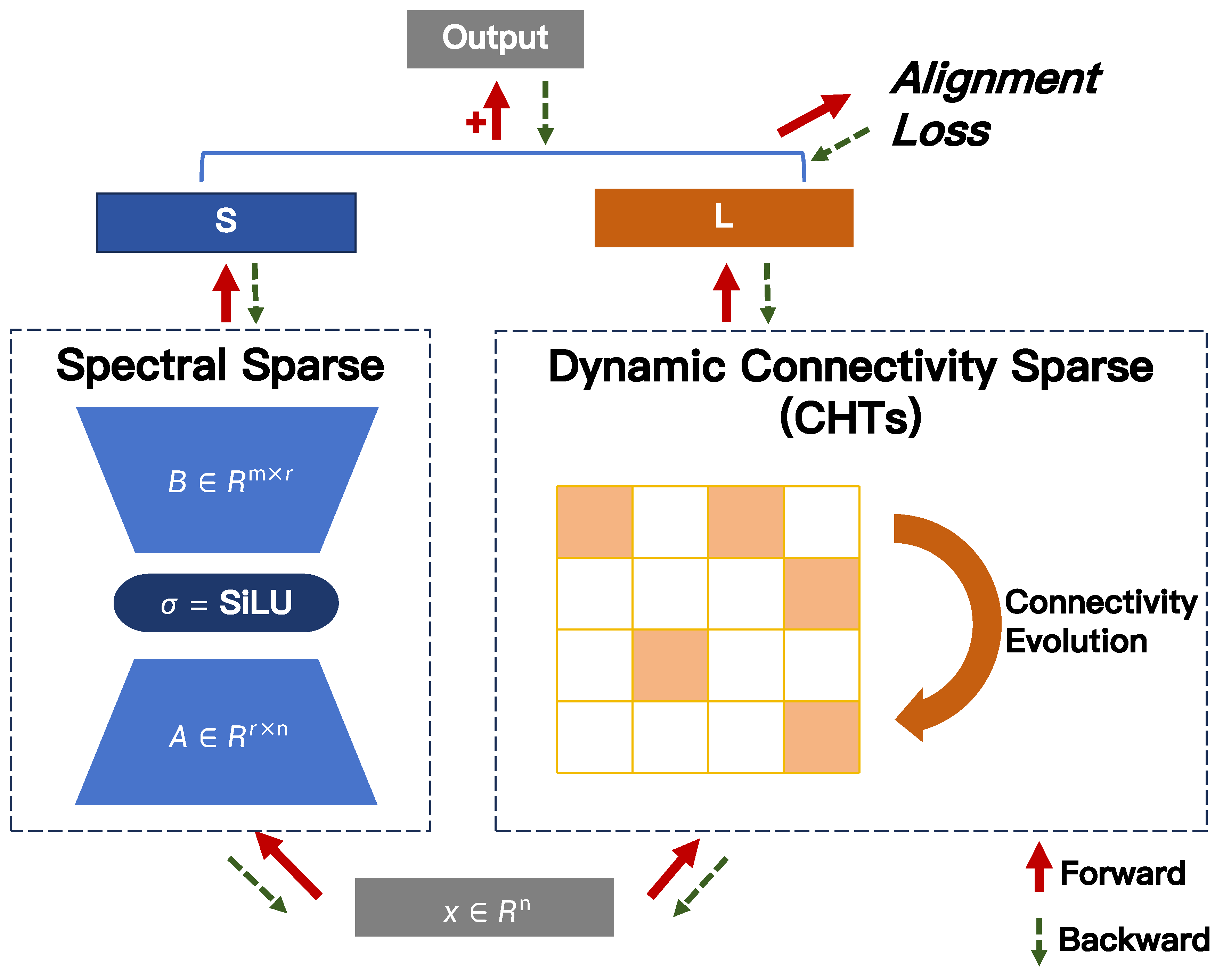
Figure 2.
The layer-wise OCR plot of LLaMA60M on OpenWebText with a total sparsity of 0.9, with sparsity-configuration . Each subplot in the figure reports the changes of OCR over training steps. The plot is based on the experiment of the first row of Table 1. For space limit, we report here the self-attention layers in the model, where each column refers to Q, K, V, O respectively.
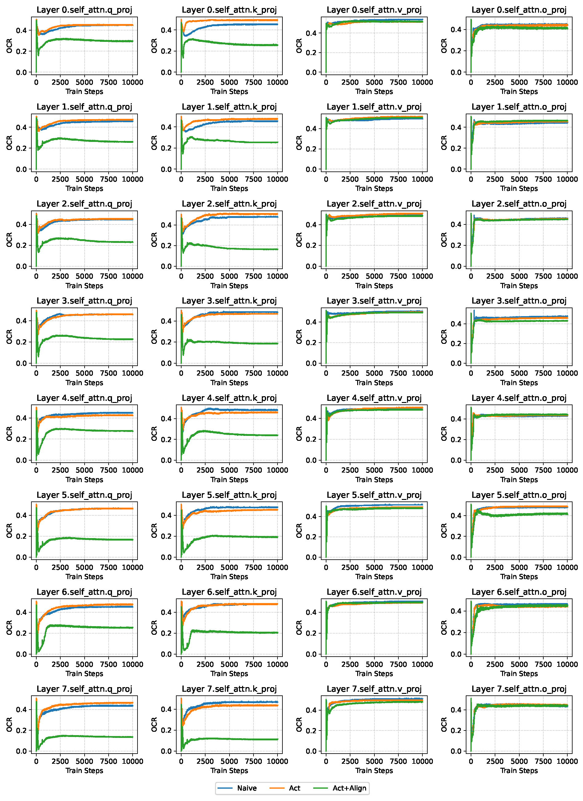
Figure 3.
Sensitivity analysis of sparsity configurations under a total sparsity of 0.7. The sparsity-configuration is defined by the sparsity s in the connectivity-sparse branch and the rank r in the low-rank branch. Each subplot illustrates the variation of validation perplexity (PPL↓) as the rank decreases by step of 5% total sparsity. Outliers with PPL values exceeding the corresponding thresholds are highlighted in red, with their true values explicitly annotated.
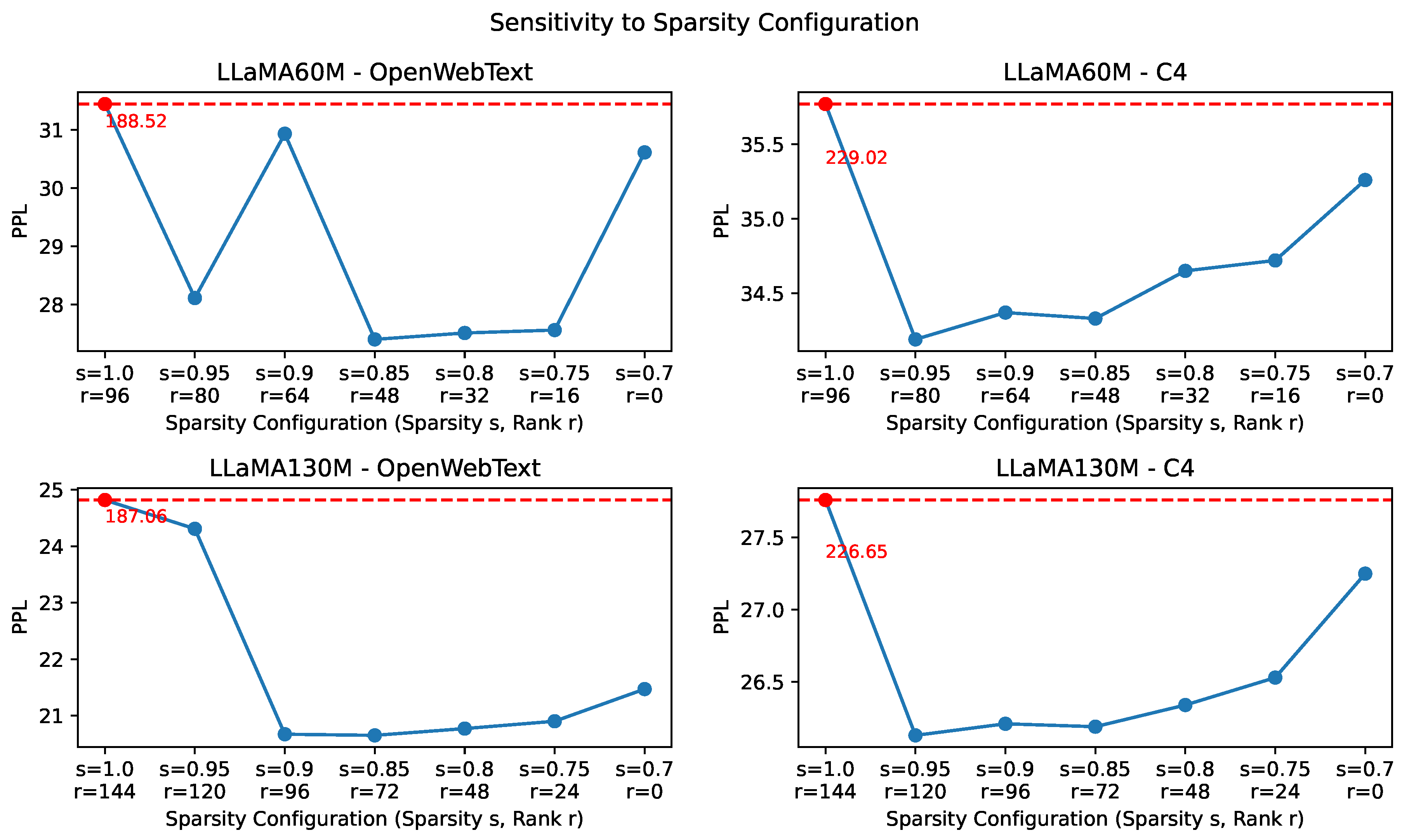
Table 1.
Comparison between different integration strategies. The table consists of two parts: a. The performance of different integration strategies, reported in terms of validation perplexity (PPL↓). The Naive strategy corresponds to a simple sum of CHTs and low-rank factorization. The Act strategy applies activation adjustment to the low-rank factorization branch. The Act+Align strategy combines activation adjustment with the alignment loss. The coefficient of the alignment loss is reported in Section 4.5. The sparsity configuration is set such that the sparse branch and the low-rank branch have the same number of trainable parameters (). b. The Wilcoxon signed-rank test p-values, which indicate whether the differences in performance between strategies are statistically significant.
| Model | Dataset | Total Sparsity | Naive | Act | Act+Align |
|---|---|---|---|---|---|
| LLaMA-60M | OpenWebText | 0.9 | 32.64 | 32.21 | 31.77 |
| 0.8 | 33.35 | 29.42 | 29.11 | ||
| 0.7 | 27.89 | 29.94 | 27.40 | ||
| C4 | 0.9 | 189.55 | 39.66 | 39.29 | |
| 0.8 | 36.71 | 36.54 | 36.16 | ||
| 0.7 | 591.42 | 34.55 | 34.33 | ||
| LLaMA-130M | OpenWebText | 0.9 | 119.35 | 24.45 | 24.07 |
| 0.8 | 22.11 | 21.98 | 21.87 | ||
| 0.7 | 21.12 | 20.90 | 20.65 | ||
| C4 | 0.9 | 30.77 | 30.30 | 30.03 | |
| 0.8 | 27.83 | 27.68 | 27.59 | ||
| 0.7 | 920.16 | 26.55 | 26.19 | ||
| Wilcoxon signed-rank | against Naive | \ | 0.0093 | 4.88e-4 | |
| p-value | against Act | \ | \ | 4.88e-4 | |
Table 2.
Validation perplexity of different methods. Validation perplexity (PPL↓) is reported in this table for different methods on different datasets under the same constraint of total sparsity . Bold values are the best performance out of all sparse methods.
Table 2.
Validation perplexity of different methods. Validation perplexity (PPL↓) is reported in this table for different methods on different datasets under the same constraint of total sparsity . Bold values are the best performance out of all sparse methods.
| Dataset | Method | LLaMA-60M | LLaMA-130M | ||||
|---|---|---|---|---|---|---|---|
| =0.9 | =0.8 | =0.7 | =0.9 | =0.8 | =0.7 | ||
| OpenWebText | Dense | 26.56 | 19.46 | ||||
| SET | 35.26 | 30.69 | 31.77 | 25.70 | 23.20 | 22.03 | |
| RigL | 45.34 | 41.33 | 39.96 | 41.25 | 44.49 | 70.11 | |
| MEST | 33.6 | 29.94 | 28.26 | 25.59 | 22.93 | 21.63 | |
| CHTs | 33.03 | 29.84 | 28.12 | 24.75 | 22.67 | 21.48 | |
| CoLA | 37.58 | 30.87 | 28.53 | 27.67 | 23.86 | 22.18 | |
| SLTrain | 33.90 | 29.83 | 27.86 | 25.33 | 22.81 | 21.25 | |
| CHTsL | 31.77 | 29.11 | 27.40 | 24.07 | 21.87 | 20.65 | |
| C4 | Dense | 33.21 | 24.55 | ||||
| SET | 42.32 | 37.70 | 35.62 | 32.45 | 29.47 | 27.75 | |
| RigL | 53.39 | 48.59 | 47.34 | 43.57 | 55.82 | 64.93 | |
| MEST | 41.46 | 37.28 | 35.40 | 32.54 | 29.29 | 27.59 | |
| CHTs | 40.62 | 37.55 | 35.23 | 31.00 | 28.69 | 27.46 | |
| CoLA | 46.41 | 38.58 | 35.87 | 33.52 | 29.26 | 27.25 | |
| SLTrain | 41.05 | 37.00 | 34.89 | 31.38 | 28.28 | 26.78 | |
| CHTsL | 39.29 | 35.95 | 34.19 | 30.03 | 27.59 | 26.19 | |
Disclaimer/Publisher’s Note: The statements, opinions and data contained in all publications are solely those of the individual author(s) and contributor(s) and not of MDPI and/or the editor(s). MDPI and/or the editor(s) disclaim responsibility for any injury to people or property resulting from any ideas, methods, instructions or products referred to in the content. |
© 2025 by the authors. Licensee MDPI, Basel, Switzerland. This article is an open access article distributed under the terms and conditions of the Creative Commons Attribution (CC BY) license (http://creativecommons.org/licenses/by/4.0/).
Copyright: This open access article is published under a Creative Commons CC BY 4.0 license, which permit the free download, distribution, and reuse, provided that the author and preprint are cited in any reuse.


