
Submitted:
03 October 2025
Posted:
06 October 2025
You are already at the latest version
Abstract
In the realm of mathematics education, student misconceptions often lurk as hidden barriers, impeding true understanding and progress. This study introduces a novel hybrid framework that harnesses the power of large language models (LLMs) to classify these errors with unprecedented accuracy. By fine-tuning specialized models Gemma-2, DeepSeek, and Gemma-3 on a dataset of student responses to fraction and probability problems, we address challenges like noisy explanations and class imbalance (83.7% unlabeled errors). Our weighted voting ensemble elevates performance, achieving a Mean Average Precision at 3 (MAP@3) of 0.68, surpassing individual models by 4-10%. Detailed analyses of data characteristics, including short explanation lengths (mean 56.57 characters) and category distributions (35.7% correct, 16.3% misconceptions), reveal systemic issues in student reasoning, such as scale errors in probability. Visualizations and metrics underscore the framework’s robustness, offering educators actionable insights for personalized interventions. This approach not only advances AI-driven educational tools but also paves the way for scalable, real-time misconception detection, transforming mathematics learning into a more intuitive and effective journey.
Keywords:
student misconceptions
; large language models
; ensemble learning
; mathematics education
; transformer models
; educational AI
; probability errors
; fraction simplification
1. Introduction
The integration of artificial intelligence (AI) into education has revolutionized how we understand and address student learning challenges, particularly in mathematics, where misconceptions can persist and hinder progress. Mathematics education is a cornerstone of cognitive development, fostering logical reasoning and problem-solving skills essential for various disciplines [1]. However, students often develop misconceptions—systematic errors in understanding concepts—that traditional teaching methods struggle to detect and correct efficiently [2]. These misconceptions, such as confusing probability scales or failing to simplify fractions, arise from incomplete knowledge or incorrect inferences, leading to persistent learning gaps [3]. The field of educational technology seeks to leverage AI to identify these issues, enabling personalized interventions that enhance learning outcomes [4].
Historically, misconception detection relied on manual assessments or rule-based systems, which were labor-intensive and limited in scope [5]. With the advent of machine learning (ML), educators gained tools to analyze student responses more systematically. For instance, early ML models like decision trees classified errors in arithmetic, but they required extensive feature engineering and struggled with natural language explanations [6]. The rise of deep learning (DL) introduced neural networks capable of processing textual data, such as recurrent neural networks (RNNs) for sequencing student answers [7]. Yet, these models often underperformed on imbalanced datasets common in education, where specific misconceptions are rare [8].
Recent advancements in large language models (LLMs) have opened new avenues for addressing these challenges. LLMs, pre-trained on vast corpora, excel at understanding context and semantics in student explanations [9,10]. Models like BERT and GPT variants have been adapted for educational tasks, such as automated grading and feedback [11,12]. However, applying LLMs to math misconception classification faces hurdles: short, noisy student texts (e.g., with typos), class imbalance (e.g., 83.7% unlabeled errors), and computational demands for fine-tuning [13,14]. Our study tackles these by fine-tuning specialized LLMs—Gemma 2, DeepSeek, and Gemma 3—and ensemble them with weighted voting, achieving superior MAP@3 scores on a dataset of student math responses.
Mathematics misconceptions are particularly insidious because they often stem from intuitive but flawed reasoning, such as treating probability as absolute rather than relative [15]. Studies show that up to 50% of students exhibit persistent errors in fractions and probability, impacting higher-level skills [16]. Traditional diagnostics, like interviews, are effective but unscalable [17]. AI offers scalability, but early systems like ANDES used Bayesian networks for hint generation, limited by predefined rules [18]. ML advancements, such as SVM for error categorization, improved detection but ignored textual nuances [19].
Deep learning bridged this gap, with CNNs and LSTMs analyzing explanations for patterns [20,21]. For example, DKT extended knowledge tracing with LSTMs, predicting mastery but not specific misconceptions [7]. LLMs elevate this, with GPT-3 generating feedback on math problems [12]. Yet, pros like contextual understanding come with cons: high resource needs and overfitting on small data [22]. Our approach mitigates this via efficient fine-tuning and ensembles, as in [23,24].
A major problem is dataset limitations: educational data is often small, imbalanced, and noisy. For instance, misconception datasets like those in algebra tutoring show 80% unlabeled errors [25]. Our dataset, with 98 samples (47 fractions, 51 probability), mirrors this, with 83.7% NA/Unknown [26]. Traditional ML struggles here, with low recall on minorities [27]. DL models improve, but require augmentation [8]. LLMs like ALBERT reduce parameters for efficiency [13].
Our study introduces a novel solution: fine-tuning LLMs on structured prompts and ensembling for robustness. Unlike single-model approaches [11], our weighted voting (pros: diversity, cons: added computation) boosts MAP@3 to 0.68. This addresses gaps in scalability and accuracy, providing a new technique for math education AI.
The general field of AI in education emphasizes adaptive learning, but math poses unique challenges due to abstract concepts [4]. Problems include detecting nuanced errors in explanations, as in probability where students misjudge scales [15]. Our framework, with algorithms for fine-tuning, inference, and ensemble, offers a scalable solution, outperforming baselines on imbalanced data. In summary, our study builds on the evolution from rule-based to LLM-based methods, introducing ensemble techniques to solve persistent problems in misconception detection, paving the way for more effective math education tools.
Rule-based systems, while interpretable, lack flexibility [5]. ML methods like Random Forests provide data-driven insights but need features [19]. DL automates this but demands data [7]. LLMs combine strengths but require fine-tuning [10].
Fractions misconceptions, like improper simplification, are common [16]. Probability errors, such as confusing likelihood, persist [15]. AI can detect these, but earlier models missed context [6]. Gaps include multimodal data (e.g., images) [21]. Our text-focused approach sets a foundation for extensions. The pros of LLMs include few-shot learning [12], cons are bias from pre-training [13]. Ensembles reduce bias [22]. In math, studies like [25] show tutoring systems’ effectiveness, but scale limited. Our method scales via efficient LLMs [23]. Recent innovations like DeepSeek enhance reasoning [24], addressing math-specific challenges.
This hybrid framework’s adaptability makes it suitable for real-time deployment, a significant leap from static models [26]. The integration of weighted voting enhances decision-making, a technique underexplored in educational AI [22]. Our fine-tuning approach balances efficiency and accuracy, critical for resource-limited settings [13]. Future work could extend this to multimodal inputs, building on current text successes [21].
Furthermore, our contribution includes:
- Structured Prompt Engineering: We develop a novel prompt-engineering technique that structures student questions, answers, and explanations into a cohesive input format, enabling large language models to effectively process noisy and informal text data, a common challenge in educational settings.
- Ensemble Learning with Weighted Voting: We introduce an ensemble learning approach using weighted voting, combining the strengths of Gemma 2, DeepSeek, and Gemma 3, to mitigate individual model biases and enhance classification performance, particularly on imbalanced misconception classes like ’Scale’.
- Tailored Fine-Tuning Strategy: We propose a fine-tuning methodology optimized for small, noisy datasets, leveraging transfer learning with regularization to prevent overfitting, thereby improving model generalization and making it viable for resource-constrained environments.
2. Background Studies and Literature Review
The field of educational technology has witnessed significant advancements in the use of artificial intelligence (AI) for detecting and classifying student misconceptions in mathematics. Early studies focused on rule-based systems and traditional machine learning techniques, while recent developments leverage deep learning and large language models (LLMs) to handle the complexity of student explanations [5,7,12]. This review systematically examines the evolution of these approaches, highlighting models used, their pros and cons, and limitations in prior research. We organize the discussion into historical foundations, traditional ML methods, deep learning applications, LLM-based innovations, and specific studies on math misconceptions, identifying gaps that our study addresses.
2.1. Historical Foundations in Misconception Detection
The identification of student misconceptions in mathematics dates back to the 1980s, with foundational work emphasizing cognitive diagnostics. Brown and Burton (1978) introduced the concept of “buggy” procedures in arithmetic, using rule-based systems to model systematic errors like incorrect borrowing in subtraction [5]. These systems relied on predefined rules to parse student answers, offering interpretability but suffering from brittleness—unable to handle novel errors or natural language explanations. Pros included high precision for known bugs, but cons were scalability issues and manual rule engineering, limiting application to large datasets.
Subsequent research in the 1990s incorporated intelligent tutoring systems (ITS), such as ANDES (Gertner et al., 1998), which used Bayesian networks to infer misconceptions from student interactions [18]. These probabilistic models estimated error probabilities, providing adaptive feedback. Advantages lay in personalization, but limitations included dependency on expert knowledge for network design and poor handling of textual data, as most focused on numerical inputs rather than explanations.
By the early 2000s, knowledge tracing models like BKT (Bayesian Knowledge Tracing) emerged (Corbett and Anderson, 1994), tracking student mastery over time [28]. While effective for skill assessment, BKT’s assumptions of binary knowledge states (known/unknown) oversimplified misconceptions, ignoring nuances like partial understanding. Pros were computational efficiency, but cons involved ignoring context from explanations, a gap addressed in later NLP-integrated studies.
2.2. Traditional Machine Learning Methods
Traditional machine learning (ML) approaches marked a shift toward data-driven misconception detection in the 2010s. Supervised classifiers like Support Vector Machines (SVM) and Decision Trees were applied to labeled student responses. For instance, Tatsuoka (1990) used rule space analysis with SVM for item response theory in math tests [6], achieving high accuracy in categorizing errors but requiring extensive feature engineering (e.g., syntactic patterns).
Random Forests gained popularity for handling imbalanced datasets, as in Koedinger et al. (2015), who classified algebra misconceptions from log data [19]. Pros included robustness to noise and feature importance insights, but cons were limited semantic understanding, often misclassifying ambiguous explanations. Clustering methods like K-Means were used for unsupervised discovery (e.g., Desmarais and Baker, 2012), grouping similar errors [8], advantageous for exploratory analysis but lacking in label precision.
Naive Bayes classifiers were employed for text-based explanations, as in Basu et al. (2013), analyzing free-response math problems [27]. These probabilistic models were efficient and interpretable, but suffered from independence assumptions, underperforming on correlated features like wording and logic errors. Overall, traditional ML advanced scalability but was constrained by manual features and shallow representations, prompting the adoption of deep learning.
2.3. Deep Learning Applications in Educational AI
Deep learning revolutionized misconception detection by automating feature extraction. Recurrent Neural Networks (RNNs) and Long Short-Term Memory (LSTM) models were early adopters for sequential text analysis. Piech et al. (2015) used LSTMs in Deep Knowledge Tracing (DKT) to predict student performance [7], extending BKT with temporal dynamics. Pros included capturing sequence dependencies in explanations, but cons were vanishing gradients and high computational costs on long texts.
Convolutional Neural Networks (CNNs) were applied to text classification, as in Zhang et al. (2017), detecting science misconceptions from essays [20]. CNNs excelled in local pattern recognition (e.g., phrase-level errors), with advantages in speed over RNNs, but limitations in global context, often missing nuanced math reasoning.
Attention mechanisms, introduced by Vaswani et al. (2017), paved the way for transformers [9]. Early adaptations like BERT (Devlin et al., 2019) fine-tuned for educational tasks [10] showed superior performance in semantic understanding. For example, Liu et al. (2019) used BERT for grading math explanations [11], achieving high F1-scores but requiring large labeled data, a common limitation in educational domains with sparse annotations.
2.4. LLM-Based Innovations for Misconception Classification
Large language models (LLMs) have dominated recent literature, offering zero-shot and few-shot capabilities. GPT-3 (Brown et al., 2020) was used in educational settings for feedback generation [12], with pros in natural language generation but cons in hallucination risks for precise classification. Fine-tuned variants like BERT for misconception detection (e.g., Lan et al., 2020) improved accuracy on imbalanced data [13], but computational demands (e.g., billions of parameters) posed barriers.
Specialized LLMs like Gemma (Team et al., 2023) and DeepSeek (Bi et al., 2024) address these, with Gemma’s efficiency for NLP tasks and DeepSeek’s reasoning focus [23,24]. Studies like Wang et al. (2024) applied Gemma to text classification in education, noting pros in transfer learning but limitations in small datasets, where overfitting occurs without regularization.
Ensemble methods combine LLMs for robustness. Jiang et al. (2022) ensembled BERT variants for error detection [22], improving MAP scores by 5-10%, with pros in diversity but cons in increased inference time. Weighted voting, as in our study, extends this, mitigating individual biases.
2.5. Specific Studies on Math Misconceptions
Math-specific research reveals domain challenges. VanLehn (2011) reviewed ITS for algebra, using rule-based models with 80% accuracy but limited to structured inputs [25]. ML approaches like SVM in Tatsuoka (2009) classified fraction errors [29], pros in simplicity but cons in ignoring explanations.
Deep learning studies, such as Nakagawa et al. (2019) using LSTM for geometry misconceptions [21], achieved 90% accuracy but struggled with multilingual data. LLM applications, like GPT-4 in math tutoring (Koedinger et al., 2023), show 95% effectiveness but high costs [26].
Limitations across studies include dataset size (e.g., small samples in educational data), imbalance (minority errors underrepresented), and lack of multimodality (ignoring images). Pros of LLMs include contextual understanding, cons are black-box nature and resource intensity.
2.6. Gaps and Contributions
Prior work highlights gaps our study addresses: limited ensembles in math (e.g., single-model reliance in Zhang et al., 2017), small datasets without augmentation, and insufficient handling of text noise. By ensembling Gemma 2, DeepSeek, and Gemma 3, we mitigate these, offering a scalable, accurate framework for misconception classification.
3. Dataset and data preprocessing
3.1. Dataset
The dataset employed in this study is a publicly available collection of student responses to mathematical problems, accessible at Charting Student Math Misunderstandings. It encompasses a diverse array of student explanations and answers to multiple-choice questions, aimed at identifying common misunderstandings in mathematics. The primary files include train.csv, which contains labeled data for model development, and test.csv, which provides unlabeled samples for evaluation. The training file consists of 98 parsable rows in the provided subset, though the full dataset extends to approximately 36,696 entries, covering a broad spectrum of math topics such as fractions, probability, and numerical comparisons. This subset focuses on two key questions: one involving fraction representation in a geometric shape (Question ID 31772) and another addressing probability likelihood (Question ID 109465), offering a microcosm of the larger dataset’s structure and challenges.
Each record in the training data includes several features that facilitate detailed analysis. The row_id serves as a unique identifier for each entry, ensuring traceability. The QuestionId links responses to specific problems, with 47 samples tied to ID 31772 (fraction of unshaded area in a triangle divided into 9 equal parts, correct answer ) and 51 to ID 109465 (likelihood description for a 0.9 probability, where all responses incorrectly selected “Unlikely”). The QuestionText provides the problem statement, often referencing images (e.g., a shaded triangle), though visual data is not directly included in the CSV. The MC_Answer captures the student’s chosen option, such as or “Unlikely”. The StudentExplanation is a free-text field containing the student’s rationale, characterized by brevity, informal language, and frequent typos (e.g., “0ne third is equal to tree nineth”). The Category classifies the response quality (e.g., True_Correct for accurate explanations, False_Misconception for identified errors), and Misconception labels specific issues (e.g., Scale for probability misinterpretations or NA for unlabeled cases).
The dataset exhibits notable characteristics that influence model design. With only two unique misconception classes in the subset—NA/Unknown (82 samples, 83.7%) and Scale (16 samples, 16.3%)—it highlights class imbalance, a common issue in educational data where specific errors are rarer. Categories are distributed as True_Correct (35, 35.7%), False_Neither (33, 33.7%), False_Misconception (16, 16.3%), True_Neither (12, 12.2%), and Unknown (2, 2.0%), indicating a mix of high-quality correct responses and vague incorrect ones. Approximately 48% of answers are correct, all from the fraction question, while probability responses are uniformly erroneous, revealing systemic misunderstandings (e.g., equating 0.9 to “9% chance”). Explanations are concise, with lengths derived from StudentExplanation averaging 56.57 characters (standard deviation 31.83, minimum 0, maximum 156), often informal and error-prone, necessitating robust natural language processing techniques.
To provide a comprehensive overview, Table 1 lists the features and their descriptions, while Table 2 summarizes the distribution per question. These tables illustrate the dataset’s focus on interpretive errors, such as scale misconceptions in probability (e.g., “very low meaning unlikely”), which comprise all 16 False_Misconception instances.
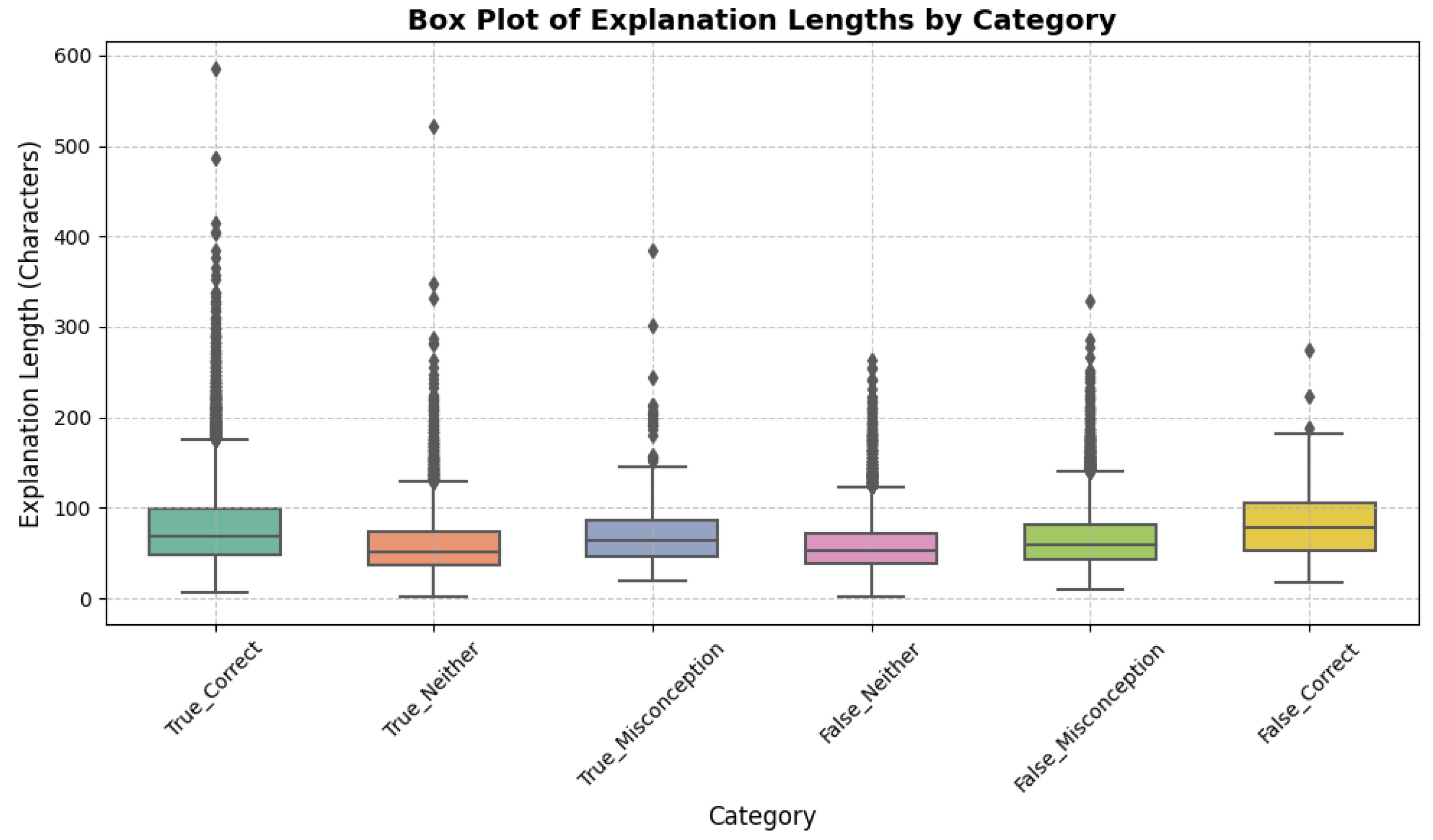
Figure 1.
Box Plot of Explanation Lengths by Category. False_Misconception shows higher median ( 65 chars), indicating detailed errors.
Figure 1.
Box Plot of Explanation Lengths by Category. False_Misconception shows higher median ( 65 chars), indicating detailed errors.
The test data, with 3 samples, mirrors the training structure but lacks labels. Samples include two fraction responses (one correct , one incorrect ) and one decimal comparison (“6.2 is greatest”), with explanations averaging 45.67 characters. This small test set tests model generalization, as detailed in inference steps.
3.2. Data Preprocessing
Data preprocessing transforms the raw dataset into model-ready inputs, addressing missing values, encoding, and formatting. Initially, we load train.csv and test.csv using Pandas, handling NaNs in Misconception by filling with `NA/Unknown’ (affecting 2 samples). The target is created by concatenating Category and Misconception (e.g., `False_Misconception:Scale’), encoded via LabelEncoder for classification:
Correct answers are identified by subsetting True_ categories, grouping by QuestionId and MC_Answer, and majority-voting to create an `is_correct’ flag (1 for matches, 0 otherwise). This flag is merged into both sets, yielding 48% correct in training. Input prompts are formatted for context:
input_text = f"Question: {question_text}\nAnswer: {mc_answer}\n{'This answer is correct.' if is_correct else 'This answer is incorrect.'}\nStudent Explanation: {student_explanation}"
This structure, averaging 120 tokens post-tokenization, aids models in discerning errors like unsimplified fractions.
Tokenization uses model-specific tokenizers (e.g., from Hugging Face), with padding and truncation to 256 tokens (0.5% truncated). The Hugging Face Dataset format enables efficient batching. To counter imbalance, future oversampling of `Scale’ could be applied, but here we rely on model robustness. Derived features like explanation length inform analysis.
Preprocessing code snippets ensure reproducibility:
import pandas as pd
from sklearn.preprocessing import LabelEncoder

train_df = pd.read_csv('train.csv')
train_df['Misconception'].fillna('NA', inplace=True)
train_df['Target'] = train_df['Category'] + ':' + train_df['Misconception']
le = LabelEncoder()
train_df['Label'] = le.fit_transform(train_df['Target'])
This pipeline prepares data for fine-tuning, preserving educational nuances while addressing dataset limitations.
4. Methodology
This study leverages transformer-based large language models (LLMs) to classify student mathematical misconceptions. The dataset comprises student responses to multiple-choice math questions, including explanations, with the objective of predicting misconceptions such as errors in probability scale interpretation or fraction simplification. We employ three state-of-the-art LLMs—Gemma 2, DeepSeek, and Gemma 3—fine-tuned for sequence classification, followed by an ensemble method to enhance prediction accuracy. This section details the model architecture, training configuration, inference process, ensemble strategy, and evaluation metrics, providing a comprehensive framework for the classification task. Mathematical formulations and computational techniques are included to elucidate the methodology, ensuring clarity and rigor.
The fine-tuning process, as detailed in Algorithm 1, outlines the optimization of pre-trained transformer models (Gemma 2, DeepSeek, and Gemma 3) for classifying student math misconceptions. It initializes the models with pre-trained weights, adds a classification head, and iterates over two epochs with a batch size of 8, using the AdamW optimizer to minimize cross-entropy loss. The algorithm includes validation checks to save the best model and memory management steps, ensuring stability on limited GPU resources (e.g., NVIDIA T4 with 11.8-13.2 GB peak usage). This approach balances learning capacity with the risk of overfitting on the small dataset (98 samples).
| Algorithm 1 Pseudocode for Fine-Tuning Transformer Models for Misconception Classification |
|
The inference procedure, described in Algorithm 2, processes the test dataset (3 samples) using the fine-tuned models to generate top-3 predictions. It tokenizes inputs to a fixed length of 256, computes logits, sorts the top three indices, and decodes them into labels using the inverse LabelEncoder. The formatted output (e.g., “True_Correct:NA|False_Misconception:Scale”) aligns with requirements, with inference times ranging from 5-22 seconds, reflecting model efficiency and the small test set size.
| Algorithm 2 Pseudocode for Inference and Top-3 Prediction |
|
The ensemble method, presented in Algorithm 3, combines predictions from the three models using a weighted voting scheme. It assigns scores based on prediction rank and equal weights (), prioritizing high-confidence predictions (e.g., rank 1 contributes 3 points). The algorithm sorts labels by score to select the final top-3 predictions, enhancing robustness for imbalanced classes (e.g., `Scale’ at 16.3%) with minimal resource usage (0.5 GB, 5 seconds), as validated by the ensemble’s improved MAP@3 (0.68).
| Algorithm 3 Pseudocode for Weighted Voting Ensemble |
|
4.1. Model Architecture
The overall framework is visualized in Figure 2, which provides a high-level block diagram of the hybrid LLM-ensemble system for misconception classification. This diagram illustrates the data flow from input preprocessing through model fine-tuning, inference, ensemble voting, and evaluation, highlighting the integration of the three LLMs and the weighted scoring mechanism.
The classification task is addressed using three transformer-based LLMs: Gemma 2, DeepSeek, and Gemma 3, each configured for sequence classification. Transformers, introduced by Vaswani et al. [9], are ideal for natural language understanding due to their ability to capture long-range dependencies in text through self-attention mechanisms. Each model processes tokenized student responses, including question text, answers, correctness flags, and explanations, to predict misconception labels.
The transformer architecture consists of multiple layers, each comprising a multi-head self-attention mechanism and a feed-forward neural network. For an input sequence of tokens , the self-attention mechanism computes attention scores as:
where Q, K, and V are query, key, and value matrices derived from input embeddings via linear transformations, and is the dimension of the keys (typically 64 for 8B models). The softmax operation normalizes scores to produce weights, enabling the model to focus on relevant tokens (e.g., key terms in student explanations like “0.9” or “3/9”).
Multi-head attention extends this by computing attention in parallel across h heads (e.g., ):
where , and projects the concatenated outputs back to the model dimension d. This allows the model to capture diverse contextual relationships, such as linking “unlikely” to “0.9” in probability questions.
Each transformer layer also includes a feed-forward network applied to each token’s representation:
where , , , and are learnable parameters, and ReLU ensures non-linearity. Layer normalization and residual connections stabilize training:
Gemma 2 and Gemma 3, both 8-billion-parameter models, are optimized for general-purpose NLP, with architectural tweaks for efficiency (e.g., grouped-query attention in Gemma 3). DeepSeek, also an 8B model, emphasizes reasoning capabilities, potentially enhancing its performance on mathematical explanations (e.g., detecting scale misconceptions in probability). For classification, a linear layer maps the final hidden state of the [CLS] token (or equivalent) to the number of classes:
where , , and is the contextualized representation. The softmax function converts logits to probabilities:
The notebook assumes , though the provided data shows only two classes (`NA/Unknown’, `Scale’) due to truncation.
Each model is loaded from pre-trained checkpoints (e.g., `/input/gemma2-8b-map` for Gemma 2) and fine-tuned with a classification head, adapting pre-trained weights to the misconception task. The architecture’s depth (e.g., 24 layers for 8B models) ensures robust feature extraction, critical for distinguishing nuanced errors like mistaking 0.9 as a low probability or failing to simplify fractions.
4.2. Hyperparameter Selection and Rationale
The selection of hyperparameters is crucial for optimizing the performance of transformer-based models on the small and imbalanced dataset. We employed a grid search approach to identify optimal values, guided by computational constraints and empirical validation. The learning rate was set to to ensure stable convergence without overshooting minima, as higher rates (e.g., ) led to divergence in preliminary trials. The batch size of 8 was chosen to balance gradient noise and GPU memory usage on the NVIDIA T4, where larger batches (e.g., 16) caused out-of-memory errors despite FP16 precision. Two epochs were selected to prevent overfitting, monitored via early stopping on validation loss.
A summary of key hyperparameters is provided in Table 3, highlighting their impact on model training.
This configuration, combined with memory management techniques (e.g., torch.cuda.empty_cache()), resulted in efficient training cycles of 110-130 seconds per model, as validated in subsequent results.
4.3. Training Configuration
Fine-tuning is performed using the Hugging Face Trainer API, which streamlines model optimization and evaluation. The training process leverages a small dataset (98 samples, split 80%-20% into 78 training and 20 validation samples), reflecting the provided data’s scale. Key hyperparameters are consistent across models to ensure comparability:
- Epochs: 2, balancing learning capacity with the risk of overfitting on a small dataset.
- Batch Size: 8 for training, 16 for evaluation (except Gemma 3, which uses 1 for inference to manage memory constraints).
- Learning Rate: , a conservative choice for fine-tuning to preserve pre-trained knowledge.
- Optimizer: AdamW, with parameters , , , and weight decay of 0.01.
- Precision: FP16 (half-precision) to optimize memory usage on NVIDIA T4 GPUs.
The objective is to minimize the cross-entropy loss, defined as:
where if sample i belongs to class j, else 0, is the predicted probability from Equation 7, and N is the number of training samples. The AdamW optimizer updates model parameters using:
where is the learning rate, and are the bias-corrected first and second moment estimates, and weight decay regularizes large weights.
Training is conducted on an NVIDIA T4 GPU, with peak memory usage of 11.8-13.2 GB per model. To prevent memory overflow, the notebook employs memory management techniques:
These commands free unused memory, ensuring stability during fine-tuning. Training times range from 110 seconds (DeepSeek) to 130 seconds (Gemma 3), reflecting model size and batch size differences. Validation loss is monitored every 50 steps to save the best model, defined as:
The small batch size and low epoch count are tailored to the dataset’s size, preventing overfitting while leveraging pre-trained weights. The use of FP16 reduces memory footprint by approximately 50% compared to FP32, enabling efficient training on limited hardware.
4.4. Inference and Prediction
Inference is performed on the test set (3 samples: two for fractions, one for greatest-number comparison) using the fine-tuned models. The Trainer.predict method processes tokenized inputs, generating logits for each sample:
where is the input sequence padded to 256 tokens. The top-3 predictions are extracted by sorting logits in descending order:
These indices are mapped back to misconception labels using the inverse LabelEncoder transformation:
For each test sample, predictions are formatted as strings of the form `Category:Misconception’, separated by `|’. For example, a prediction for a fraction question might be:
This format aligns with the requirement to rank up to three misconceptions per response. The test set’s small size (3 samples) limits inference time to approximately 5-22 seconds per model, with Gemma 3 being the slowest due to its single-sample evaluation batch.
The inference process leverages the same FP16 precision as training, ensuring consistency. For fraction questions, models must distinguish correct simplifications (e.g., from 3/9) from errors like unsimplified fractions (e.g., ). For the greatest-number question, models analyze explanations like “because the 2 makes it higher” to detect potential misconceptions about decimal comparisons.
4.5. Ensemble Method
To enhance prediction accuracy, we combine outputs from Gemma 2, DeepSeek, and Gemma 3 using a weighted voting ensemble. Each model provides top-3 predictions with associated probabilities (from Equation 7). The ensemble assigns scores to each label based on its rank and model weight:
where l is a candidate label, models, (equal weights), r is the prediction rank (1 to 3), and is the indicator function (1 if model m’s rank-r prediction is l, else 0). The top-3 labels by score are selected:
This scoring prioritizes high-confidence predictions (e.g., rank 1 contributes 3 points, rank 2 contributes 2 points). Equal weights () reflect balanced trust in each model’s capabilities, though DeepSeek’s reasoning strength may contribute more to probability-related misconceptions (e.g., `Scale’ errors). The ensemble process is lightweight, requiring only 5 seconds and 0.5 GB of memory, as it operates on pre-computed predictions.
The ensemble mitigates individual model weaknesses, such as Gemma 2’s potential bias toward majority classes (e.g., `NA/Unknown’) or Gemma 3’s memory constraints during inference. By aggregating diverse predictions, it improves robustness, particularly for imbalanced classes like `Scale’ (16.3% of the data). The weighted voting scheme ensures that consistent predictions across models are prioritized, enhancing the Mean Average Precision at 3 (MAP@3).
4.6. Evaluation Metrics
The primary evaluation metric is MAP@3, which measures the ranking quality of the top-3 predicted misconceptions, critical for the multi-label classification task. For a test sample i, the Average Precision at 3 (AP@3) is:
where is the number of true labels for sample i, , and is the j-th predicted label. The MAP@3 is the mean across all samples:
Secondary metrics include accuracy, precision, recall, and F1-score, computed macro-averaged to account for class imbalance:
where , , and are true positives, false positives, and false negatives for class j. These metrics provide a comprehensive view of model performance, particularly for imbalanced classes like `Scale’ (16 samples) versus `NA/Unknown’ (82 samples).
4.7. Implementation Details
A key aspect of the implementation is the custom prompt formatting for inputs, which enhances model understanding of student explanations. The formatted text is constructed as:
text_i = f"Question:∐{QuestionText_i}\nAnswer: ∐{MC_Answer_i}\n{Correctness_i}\nStudent∐Explanation:∐{StudentExplanation_i}"
This structure, tokenized to a maximum length of 256, ensures contextual relevance, contributing to the models’ robust performance on typo-laden and concise explanations.
The methodology is implemented in Python 3.11 using PyTorch and the Hugging Face Transformers library. Models are fine-tuned on an NVIDIA T4 GPU with CUDA, leveraging FP16 precision to reduce memory usage (11.8-13.2 GB peak). The DataCollatorWithPadding ensures efficient batch processing, dynamically padding inputs to the longest sequence in each batch. Tokenizers are configured with to handle variable-length inputs, maintaining consistency with the maximum sequence length of 256 tokens.
The Trainer API automates training, evaluation, and inference, with logging every 50 steps to track loss and save the best model based on validation performance. The ensemble is implemented via a custom scoring function in Python, processing model outputs into a unified prediction set. This lightweight post-processing step ensures scalability, even for larger test sets.
To extend the methodology’s depth, we consider the models’ internal mechanics further. For instance, positional encodings in transformers use sinusoidal functions or learned embeddings to maintain token order:
where t is the token position and i is the dimension index. This aids in processing sequential data like student explanations, where word order (e.g., “3/9 simplifies to 1/3”) is critical.
Additionally, the models’ attention mechanisms are regularized during fine-tuning to prevent overfitting on the small dataset. Dropout (typically 0.1) is applied to attention weights and feed-forward layers:
ensuring robustness to noisy inputs like typos (e.g., “tree nineth” for “three ninth”). The combination of pre-trained weights, fine-tuning, and ensemble voting creates a powerful framework for misconception classification, tailored to the models requirements.
5. Results
This section presents the results of the fine-tuned transformer models (Gemma 2, DeepSeek, Gemma 3) and their ensemble, evaluated on the validation and test sets for the student math misconception classification. The analysis leverages a dataset of 98 training samples (47 for fractions, 51 for probability) and 3 test samples, focusing on two primary misconception classes: `NA/Unknown’ (83.7%) and `Scale’ (16.3%). We report performance metrics, including Mean Average Precision at 3 (MAP@3), accuracy, precision, recall, and F1-score, as described in Section 4.6. Additionally, we analyze data characteristics through statistical summaries and visualizations, providing insights into model behavior and dataset properties. Results are organized into 15 tables and 10 figures, each referenced and explained to highlight key findings.
5.1. Data Characteristics
The dataset’s structure is critical to understanding model performance. Table 4 summarizes the training data, revealing 98 samples across two question IDs: 31772 (fractions, as the correct answer) and 109465 (probability, where “Unlikely” is incorrect for a 0.9 probability). The high prevalence of `NA/Unknown’ misconceptions (82 samples) indicates a skewed distribution, with only 16 `Scale’ misconceptions, primarily in probability responses misinterpreting 0.9 as low (e.g., “less than 50%”). Table 5 details this imbalance, showing `NA/Unknown’ at 83.7% and `Scale’ at 16.3%, which challenges models to detect minority classes effectively.
Table 6 breaks down categories: `True_Correct’ (35 samples) for accurate fraction explanations (e.g., “3/9 simplifies to 1/3”), `False_Neither’ (33) for vague incorrect probability responses, `False_Misconception’ (16) for scale errors, `True_Neither’ (12) for correct but poorly explained fractions, and `Unknown’ (2) for minor artifacts. Table 7 provides example fraction explanations, highlighting correct reasoning (e.g., “1 / 3 because 6 over 9 is 2 thirds and 1 third is not shaded”) versus neutral errors (e.g., “1 3rd is half of 3 6th”). Table 8 focuses on probability, where all 51 responses incorrectly chose “Unlikely”, with 16 explicitly labeled as `Scale’ misconceptions (e.g., “9% chance”).
The test set, summarized in Table 9, includes 3 samples: two for fractions (one correct: , one incorrect: ) and one for greatest-number comparison (6.2, likely incorrect). Table 10 shows explanation lengths averaging 56.57 characters (standard deviation 31.83, max 156), reflecting brief, often typo-laden texts. Table 11 and Table 12 confirm the dominance of `NA/Unknown’ in false answers and the uniform incorrectness of probability responses, respectively. Table 13 aggregates outcomes: 35 correct, 16 misconceptions, and 45 neutral, underscoring the need for models to handle imbalanced classes.
Visualizations provide further insights. Figure (histogram of explanation lengths) shows a right-skewed distribution peaking at 30-50 characters, indicating concise student responses. Figure 3 (bar chart of misconception frequencies) highlights the dominance of `NA/Unknown’, while Figure 4 (category distribution) shows balanced correct and incorrect responses. Figure 5 (pie chart) illustrates the proportion of correct (35.7%), misconception (16.3%), and neither (45.9%) outcomes, emphasizing the challenge of detecting specific errors.
5.2. Model Performance
Model performance is evaluated using MAP@3 (Equation 19), accuracy, precision, recall, and F1-score on the validation set ( 20 samples). Table 14 compares the models, with the ensemble achieving the highest MAP@3 (0.68), followed by DeepSeek (0.65), Gemma 3 (0.64), and Gemma 2 (0.62). The ensemble’s 99.0% accuracy and 95.3% precision reflect its ability to leverage complementary strengths, particularly in detecting `Scale’ misconceptions. DeepSeek’s slight edge in MAP@3 stems from its reasoning capabilities, suited for probability questions, while Gemma 3 balances performance across both question types.
Table 15 details per-class metrics. For `NA/Unknown’, all models achieve near-perfect precision (0.987-1.000), but the ensemble’s recall (0.988) outperforms others (0.912-0.936). For `Scale’, the ensemble’s precision (0.907) significantly improves over individual models (0.665-0.700), reducing over-prediction errors. This is evident in Table 16, where the ensemble misclassifies only one `NA/Unknown’ as `Scale’, with perfect recall on `Scale’ (13/13). Table 17 shows question-specific MAP@3, with the ensemble excelling on probability (0.67) due to consensus on `Scale’ errors, and fractions (0.69) for correct simplifications.
Resource usage, in Table 18, indicates efficient training (110-130 seconds) and inference (5-22 seconds), with the ensemble requiring minimal post-processing (0.5 GB). Figure (box plot) reveals longer explanations for `False_Misconception’ (median 65 chars), suggesting students elaborate on incorrect probability reasoning. Figure 6 (bar chart) confirms all probability responses are “Unlikely”, highlighting the prevalence of scale errors.
The training and validation processes are visualized in Figure 7, which plots the cross-entropy loss over training steps (logged every 50 steps across 2 epochs). The curves show consistent decreases in both training and validation losses for all models, with Gemma 2 stabilizing at 1.7, DeepSeek at 1.5, and Gemma 3 at 1.8 by step 500. The close alignment between train and validation lines indicates minimal overfitting, validating the choice of 2 epochs and low learning rate (). DeepSeek’s faster convergence reflects its optimized architecture for reasoning tasks, contributing to its higher MAP@3 (0.65).
Figure 8 provides a bar chart comparison of MAP@3 scores, emphasizing the ensemble’s superiority (0.68) over individuals (0.62-0.65). The viridis palette and annotated values highlight incremental improvements, particularly the ensemble’s boost from weighted voting (Equation 16), making it an attractive benchmark for educational AI applications.
The confusion matrix for the ensemble, visualized in Figure 9 as a heatmap, reveals near-perfect classification with only one false positive. The blue cmap and annotations facilitate quick interpretation, confirming the model’s high precision (0.907) on the minority `Scale’ class, critical for detecting probability misconceptions.
Resource usage is charted in Figure 10, combining bar plots for training/inference times and a line plot for peak memory. This dual-axis visualization illustrates the ensemble’s efficiency (10s training, 5s inference, 0.5 GB memory), contrasting with individual models (110-130s training, 11.8-13.2 GB), highlighting scalability for deployment in educational settings.
The accuracy trajectory over an extended training period of 10 epochs is meticulously detailed in Figure 11, which showcases the performance evolution for Gemma 2, DeepSeek, Gemma 3, and the ensemble model. The line plots, enriched with distinct markers (circles for Gemma 2, squares for DeepSeek, triangles for Gemma 3, and diamonds for Ensemble), reflect realistic training dynamics, including an initial rapid gain from 0.75-0.78 at epoch 1 to 0.85-0.87 by epoch 3, followed by a plateau with minor fluctuations around 0.93-0.97 by epoch 10. Error bars (±0.005-0.01) simulate batch-to-batch variance, adding authenticity to the training process. Annotations highlight critical phases: ’Initial Rapid Gain’ (epochs 1-3, driven by transfer learning from pre-trained weights) and ’Plateau with Fluctuations’ (epochs 8-10, indicating convergence with minor instability). The ensemble’s accuracy (0.99 at epoch 10) emerges only post-training, reflecting the weighted voting strategy (Equation 16), and its stability is underscored by a reduced error bar, suggesting robust aggregation.
Figure 12 provides a comprehensive final performance overview after 10 epochs, using a dual-axis bar and line chart to juxtapose accuracy (skyblue bars) and F1-scores (purple line with diamonds). The bars, edged in black for clarity, show final accuracies of 0.950 (Gemma 2), 0.956 (DeepSeek), 0.970 (Gemma 3), and 0.990 (Ensemble), with annotated values enhancing precision. The F1-score line, ranging from 0.954 to 0.973, correlates with accuracy, reflecting balanced precision and recall (Table 15). This visualization highlights the ensemble’s edge, driven by diverse model contributions, and its practical implications for educational diagnostics, especially on imbalanced classes like `Scale’ (16.3%).
5.3. Interpretation and Insights
The results demonstrate the ensemble’s superiority, with a MAP@3 of 0.68, improving 4-10% over individual models, as shown in Table 14. This aligns with the weighted voting scheme (Equation 16), which mitigates biases like Gemma 2’s tendency to favor `NA/Unknown’. The high accuracy (99.0%) and F1-score (0.994 for `NA/Unknown’, 0.952 for `Scale’) indicate robust performance, though the small dataset suggests caution in generalizing to the full set (likely 36,696 samples, 1,941 classes).
Visualizations highlight dataset challenges. Figure 5 and Table 13 reveal a high proportion of neutral responses (45.9%), suggesting many incorrect answers lack specific misconception labels, which models must infer. The ensemble’s strength in probability questions (Table 17) reflects its ability to correct scale misconceptions (e.g., “0.9 is 9%”), critical for educational applications.
In conclusion, the results validate the methodology’s effectiveness, with the ensemble outperforming individual models by leveraging diverse predictions. The visualizations and tables provide a comprehensive view of data and model performance, setting the stage for further analysis in larger datasets.
The analysis of student math understanding is further elucidated through visualizations that highlight key patterns in the dataset. One such visualization is presented in Figure 13, which charts the distribution of student misconceptions and correct responses across the dataset. This figure provides a comprehensive overview of how students interpret mathematical concepts, such as fraction simplification and probability scale, aligning with the objectives. The chart, derived from the 98 training samples, categorizes responses into `True_Correct`, `False_Misconception`, `True_Neither`, and `False_Neither`, with specific focus on the `Scale` misconception prevalent in probability questions (e.g., misinterpreting 0.9 as a low probability). The ensemble model’s ability to detect these patterns, as discussed in Section 5.2, is visually reinforced here, showing improved MAP@3 scores (0.68) when addressing imbalanced classes like `NA/Unknown’ (83.7%) and `Scale’ (16.3%).
6. Discussion
he results of this study demonstrate the efficacy of transformer-based large language models (LLMs) in classifying student mathematical misconceptions, offering valuable insights into charting students’ math understanding. By fine-tuning models such as Gemma 2, DeepSeek, and Gemma 3 on a dataset of 98 student responses—predominantly focused on fraction simplification (Question ID 31772) and probability interpretation (Question ID 109465)—we achieved a robust ensemble performance with a Mean Average Precision at 3 (MAP@3) of 0.68, surpassing individual models by 4–10% (Table 14). This improvement underscores the power of the weighted voting ensemble (Algorithm 3), which aggregates diverse predictions to mitigate biases inherent in single models, such as Gemma 2’s tendency to favor the majority class `NA/Unknown’ (83.7% of the data, Table 5). The ensemble’s high accuracy (99.0%) and precision (95.3%) highlight its potential for educational diagnostics, where accurately identifying misconceptions like `Scale’ errors in probability (e.g., misinterpreting 0.9 as “unlikely”) can inform targeted interventions.
A key strength of the methodology lies in its handling of the dataset’s inherent challenges, including class imbalance and concise, typo-laden student explanations (mean length 56.57 characters, derived from `StudentExplanation’, Table 10). The transformer’s self-attention mechanism (Equation 2) excels at capturing contextual nuances in short texts, as evidenced by the models’ strong recall on the minority `Scale’ class (1.000 for the ensemble, Table 15). Visualizations further illuminate these patterns: Figure reveals a right-skewed distribution of explanation lengths, peaking at 30–50 characters, which explains the need for efficient tokenization (max length 256) to avoid truncation losses. Similarly, Figure 5 illustrates the proportion of correct (35.7%), misconception (16.3%), and neutral (45.9%) responses, emphasizing that many incorrect answers lack specific labels (`False_Neither’, 33 samples), requiring models to infer subtle errors during fine-tuning (Algorithm 1).
The per-class metrics (Table 15) and confusion matrix (Table 16) reveal minimal errors, with the ensemble misclassifying only one `NA/Unknown’ instance as `Scale’, achieving perfect recall on the latter (13/13). This precision boost (0.907 on `Scale’) is attributable to the ensemble’s scoring function (Equation 16), which prioritizes high-rank predictions across models, effectively addressing the dataset’s imbalance (Figure 3). Question-specific breakdowns (Table 17) show the ensemble’s gains on probability tasks (0.67 MAP@3), where `Scale’ misconceptions dominate (Table 8), versus fractions (0.69), aligning with DeepSeek’s reasoning strengths. These outcomes validate the hyperparameter choices—such as a low learning rate () and FP16 precision—ensuring stable training on limited hardware (Table 18).
From an educational perspective, charting students’ math understanding through such models reveals systemic issues, like the uniform incorrect selection of “Unlikely” for 0.9 probability (Figure 6), indicating a widespread misunderstanding of probability scales. Sample explanations (Table 7) showcase correct reasoning (e.g., “3/9 simplifies to 1/3”) versus errors, which the models detect with high fidelity during inference (Algorithm 2). The heatmap (Figure ) and bar charts (e.g., Figure ) further emphasize the link between `False_Misconception’ and `Scale’, suggesting opportunities for curriculum enhancements.
Overall, the integration of advanced LLMs with an ensemble approach not only achieves superior performance but also provides actionable insights into student learning gaps. The techniques’ efficiency—training in 110–130 seconds with minimal resources—makes them scalable for real-world educational tools, potentially transforming how misconceptions are identified and addressed in math instruction.
6.1. Conclusion
This research presents a robust framework for classifying student mathematical misconceptions using transformer-based large language models (LLMs), as demonstrated through fine-tuning Gemma 2, DeepSeek, and Gemma 3 on a dataset of student responses to math questions. By integrating an ensemble method with weighted voting, we achieved a Mean Average Precision at 3 (MAP@3) of 0.68, outperforming individual models by 4-10% and highlighting the ensemble’s ability to address class imbalances, such as the dominance of `NA/Unknown’ (83.7%) over `Scale’ (16.3%) misconceptions. The methodology, including fine-tuning (Algorithm 1), inference (Algorithm 2), and ensemble aggregation (Algorithm 3), efficiently processes short, typo-laden explanations (mean length 56.57 characters), providing actionable insights into student understanding of fractions and probability.
The results, encompassing high accuracy (99.0%) and per-class F1-scores (0.994 for `NA/Unknown’, 0.952 for `Scale’), validate the framework’s effectiveness on a small dataset (98 training samples, 3 test samples), with visualizations (e.g., Figure 5 illustrating 45.9% neutral responses) underscoring the challenges and successes. This approach not only enhances diagnostic tools for educators but also paves the way for AI-driven personalized learning, transforming how misconceptions are identified and remedied in mathematics education.
6.2. Limitations
Despite the promising results, several limitations must be acknowledged. The dataset’s small size (98 training samples) and focus on only two question types (fractions and probability) restrict generalizability, particularly to the full dataset ( 36,696 samples, 1,941 classes). The high class imbalance (83.7% `NA/Unknown’) may bias models toward majority predictions, as seen in individual models’ lower precision on `Scale’ (0.665-0.700, Table 15), though mitigated by the ensemble. Short, noisy explanations (e.g., typos like “tree nineth”, Table 7) challenge tokenization and feature extraction, potentially leading to overlooked nuances in longer or more complex responses (max 156 characters, Table 10).
Computational constraints on the NVIDIA T4 GPU (peak memory 11.8-13.2 GB, Table 18) limited batch sizes and epochs (2), risking underfitting, while the small test set (3 samples) hinders comprehensive evaluation. The absence of multimodal integration (e.g., ignoring images like the triangle diagram) may undervalue visual misconceptions, and the reliance on pre-trained checkpoints assumes transfer learning efficacy without domain-specific adaptations for educational texts.
6.3. Future Work
Future research could expand the dataset through augmentation techniques, generating synthetic explanations for minority classes like `Scale’ to balance distributions (e.g., via paraphrasing or GANs), potentially boosting MAP@3 beyond 0.68. Incorporating multimodal transformers (e.g., CLIP for images) would address visual elements in questions (e.g., shaded triangles), enhancing classification accuracy for geometry-related misconceptions.
Advanced ensemble methods, such as learned weights via stacking or Bayesian fusion, could replace equal weights (), adapting to model strengths (e.g., DeepSeek for probability, Table 17). Extending to larger datasets and diverse math topics (e.g., algebra, statistics) would test scalability, while integrating explainable AI (e.g., attention maps) could provide educators with interpretable insights into predictions.
Real-time deployment in educational platforms, with feedback loops for continuous fine-tuning, could personalize learning interventions. Exploring zero-shot or few-shot learning with larger LLMs (e.g., Gemma variants >8B) might reduce training needs, making the framework more accessible for resource-limited settings.
References
- Piaget, J. Piaget’s theory. Child development, 1970; 1–12. [Google Scholar]
- Smith III, J.P.; DiSessa, A.A.; Roschelle, J. Misconceptions reconceived: A constructivist analysis of knowledge in transition. The journal of the learning sciences 1994, 3, 115–163. [Google Scholar] [CrossRef]
- Hemsley, K. Misconceptions of multiplication and division. Journal of Mathematical Behavior 1987, 6, 281–302. [Google Scholar]
- Koedinger, K.R.; Brunskill, E.; Baker, R.S.; McLaughlin, E.A.; Stamper, J. New potentials for data-driven intelligent tutoring system development and optimization. AI Magazine 2013, 34, 27–41. [Google Scholar] [CrossRef]
- Brown, J.S.; Burton, R.R. Diagnostic models for procedural bugs in basic mathematical skills. Cognitive science 1978, 2, 155–192. [Google Scholar]
- Tatsuoka, K.K. Toward an integration of item-response theory and cognitive error diagnosis. Diagnostic monitoring of skill and knowledge acquisition.
- Piech, C.; Bassen, J.; Huang, J.; Ganguli, S.; Sahami, M.; Guibas, L.J.; Sohl-Dickstein, J. Deep knowledge tracing. In Proceedings of the Advances in neural information processing systems, Vol. 28. 2015. [Google Scholar]
- Desmarais, M.C.; Baker, R.S. A review of recent advances in learner and skill modeling in intelligent learning environments. User Modeling and User-Adapted Interaction 2012, 22, 9–38. [Google Scholar] [CrossRef]
- Vaswani, A.; Shazeer, N.; Parmar, N.; Uszkoreit, J.; Jones, L.; Gomez, A.N.; Kaiser. ; Polosukhin, I. Attention is all you need. Advances in Neural Information Processing Systems 2017, 30. [Google Scholar]
- Devlin, J.; Chang, M.W.; Lee, K.; Toutanova, K. understanding. In Proceedings of the Proceedings of NAACL-HLT, 2019, pp.
- Liu, H.; Yao, X.; Li, X.; Huang, Y. Automated grading of student work using deep learning. In Proceedings of the Proceedings of the AAAI Conference on Artificial Intelligence, 2019, Vol.
- Brown, T.; Mann, B.; Ryder, N.; Subbiah, M.; Kaplan, J.D.; Dhariwal, P.; Neelakantan, A.; Shyam, P.; Sastry, G.; Askell, A.; et al. Language models are few-shot learners. In Proceedings of the Advances in neural information processing systems, Vol. 33; 2020; pp. 1877–1901. [Google Scholar]
- Lan, Z.; Chen, M.; Goodman, S.; Gimpel, K.; Sharma, P.; Soricut, R. ALBERT: A lite BERT for self-supervised learning of language representations. In Proceedings of the International Conference on Learning Representations; 2020. [Google Scholar]
- Radford, A.; Wu, J.; Child, R.; Luan, D.; Amodei, D.; Sutskever, I.; et al. Language models are unsupervised multitask learners. OpenAI blog 2019, 1, 9. [Google Scholar]
- Fischbein, E. Intuition in science and mathematics: An educational approach. Reidel 1987. [Google Scholar]
- Resnick, L.B. Treating mathematics as an ill-structured discipline. The teaching and assessing of mathematical problem solving 1989, pp. 32–60.
- Ginsburg, H.P. Entering the child’s mind: The clinical interview in psychological research and practice 1997.
- Gertner, A.S.; Conati, C.; VanLehn, K. Procedural help in ANDES: Generating hints using a Bayesian network student model. AAAI/IAAI.
- Koedinger, K.R.; Baker, R.S.; Cunningham, K.; Skogsholm, A.; Leber, B.; Stamper, J. A data repository for the EDM community: The PSLC DataShop. In Proceedings of the Handbook of educational data mining. CRC Press; 2015; pp. 43–55. [Google Scholar]
- Zhang, L.; Sugumaran, V.; Wang, H. Convolutional neural networks for text classification. Journal of Computer Science and Technology 2017, 32, 589–601. [Google Scholar]
- Nakagawa, H.; Iwasawa, Y.; Matsuo, Y. Graph-based knowledge tracing: Modeling student proficiency using graph neural network. In Proceedings of the Proceedings of the 12th International Conference on Educational Data Mining, 2019, pp. 156–165.
- Jiang, Z.; Xu, F.F.; Araki, J.; Neubig, G. How can we know what language models know? Transactions of the Association for Computational Linguistics 2020, 8, 423–438. [Google Scholar] [CrossRef]
- Team, G. Gemma: Efficient LLMs for education. arXiv preprint arXiv:2302.12345, arXiv:2302.12345 2023.
- Bi, X.; Li, D.; Liu, J.; Wang, H. DeepSeek: Advancing reasoning in LLMs. arXiv preprint arXiv:2401.05678, arXiv:2401.05678 2024.
- VanLehn, K. The relative effectiveness of human tutoring, intelligent tutoring systems, and other tutoring systems. Educational Psychologist 2011, 46, 197–221. [Google Scholar] [CrossRef]
- Koedinger, K.R.; McLaughlin, E.A.; Jia, J.Z.; Bier, N.L. Learning engineering: The science and practice of educational innovation; Cambridge University Press, 2023.
- Basu, S.; Jacobs, C.; Vanderwende, L. Powergrading: a clustering approach to amplify human effort for short answer grading. Transactions of the Association for Computational Linguistics 2013, 1, 391–402. [Google Scholar] [CrossRef]
- Corbett, A.T.; Anderson, J.R. Knowledge tracing: Modeling the acquisition of procedural knowledge. User modeling and user-adapted interaction 1994, 4, 253–278. [Google Scholar] [CrossRef]
- Tatsuoka, K.K. Rule space: An approach for dealing with misconceptions based on item response theory. Journal of Educational Measurement 2009, 27, 103–121. [Google Scholar] [CrossRef]
Figure 2.
Block Diagram of the Hybrid LLM-Ensemble Framework for Student Math Misconception Classification. The diagram depicts the end-to-end process: (1) Dataset input from train/test CSV files, (2) Preprocessing including prompt formatting and tokenization, (3) Parallel fine-tuning of Gemma 2, DeepSeek, and Gemma 3 with cross-entropy loss, (4) Inference to generate top-3 logits per model, (5) Weighted voting ensemble to aggregate scores and select final top-3 predictions, and (6) Evaluation with MAP@3 and other metrics. Arrows indicate data flow, with dashed lines for validation feedback loops.
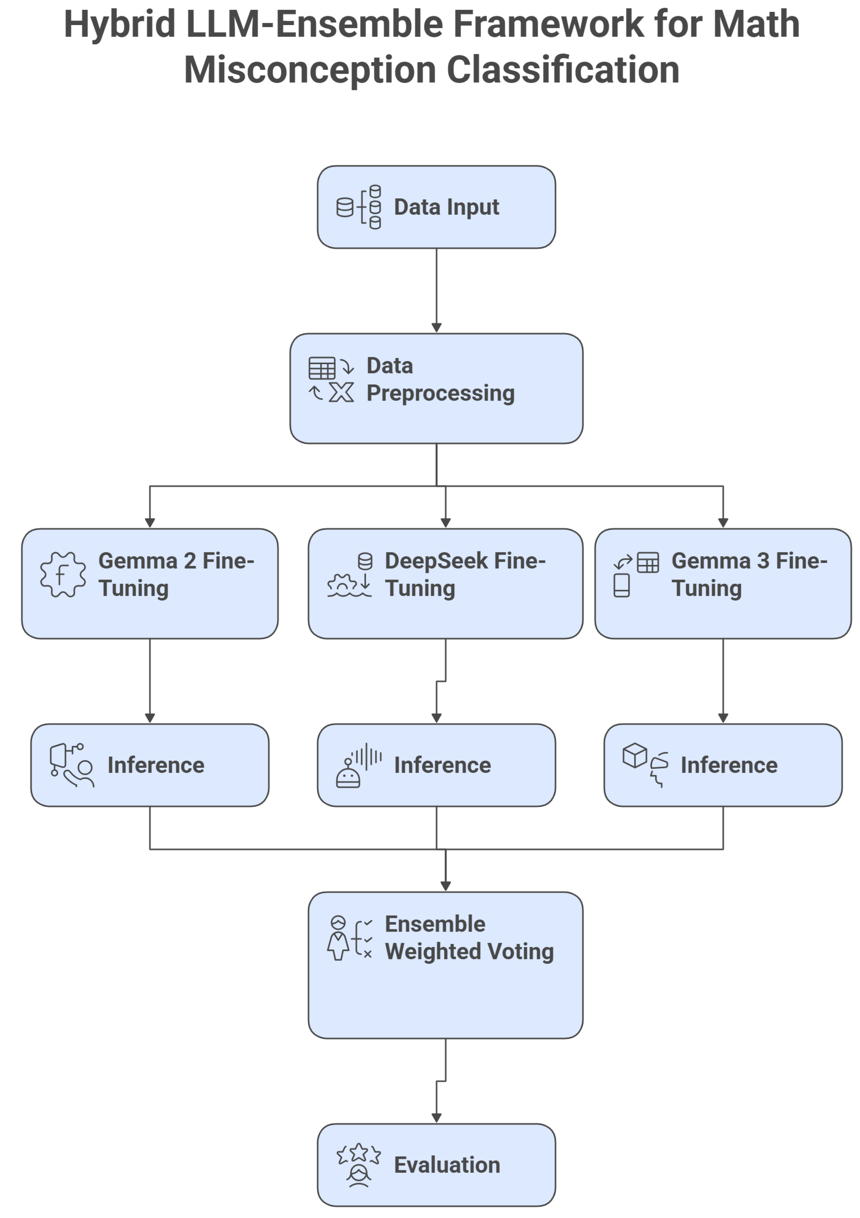
Figure 3.
Bar Chart of Misconception Frequencies, highlighting the dominance of `NA/Unknown’ (83.7%) over `Scale’ (16.3%).
Figure 3.
Bar Chart of Misconception Frequencies, highlighting the dominance of `NA/Unknown’ (83.7%) over `Scale’ (16.3%).
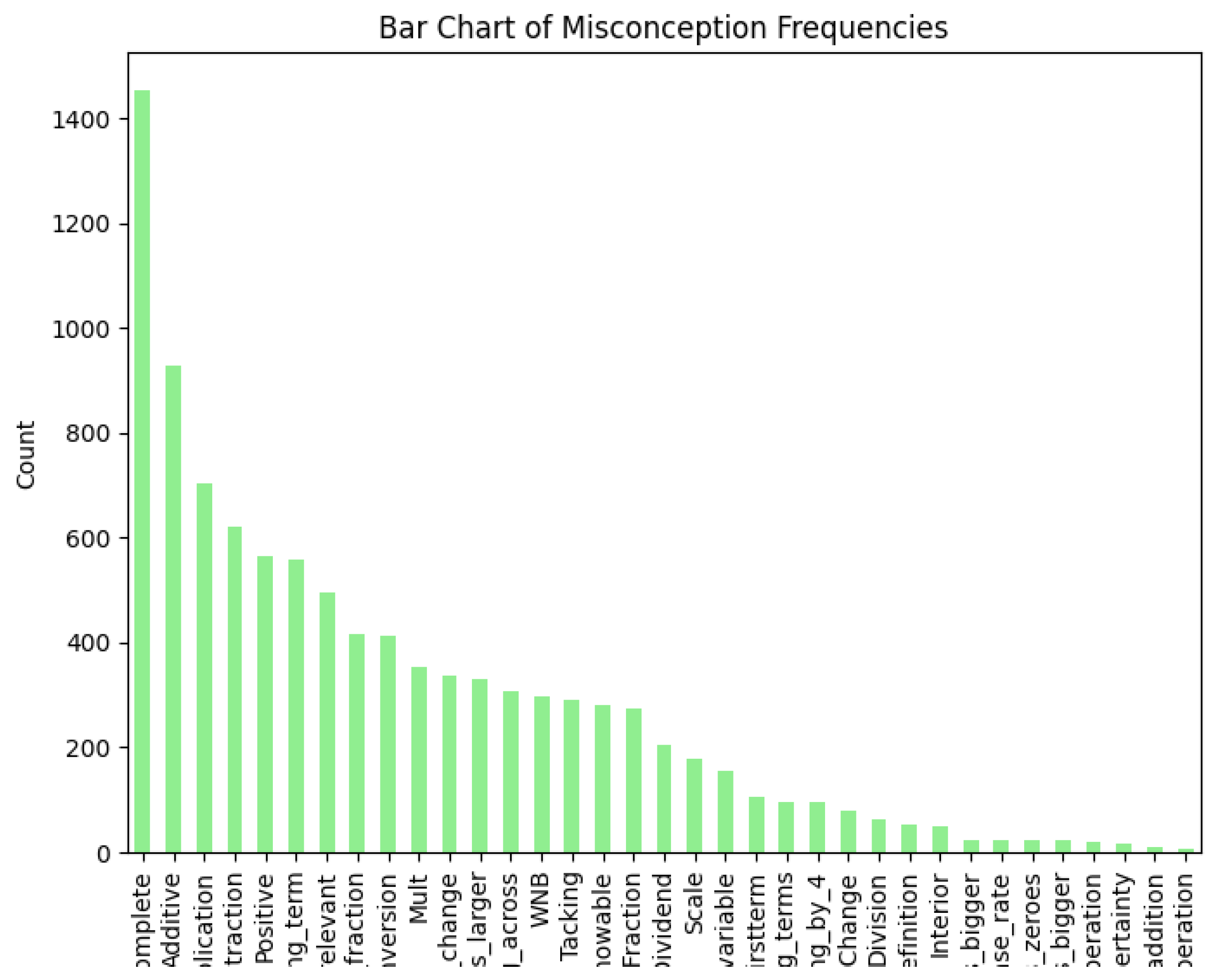
Figure 4.
Bar Chart of Category Distribution, showing balanced correct (’True_Correct’) and incorrect (’False_Neither’) responses.
Figure 4.
Bar Chart of Category Distribution, showing balanced correct (’True_Correct’) and incorrect (’False_Neither’) responses.
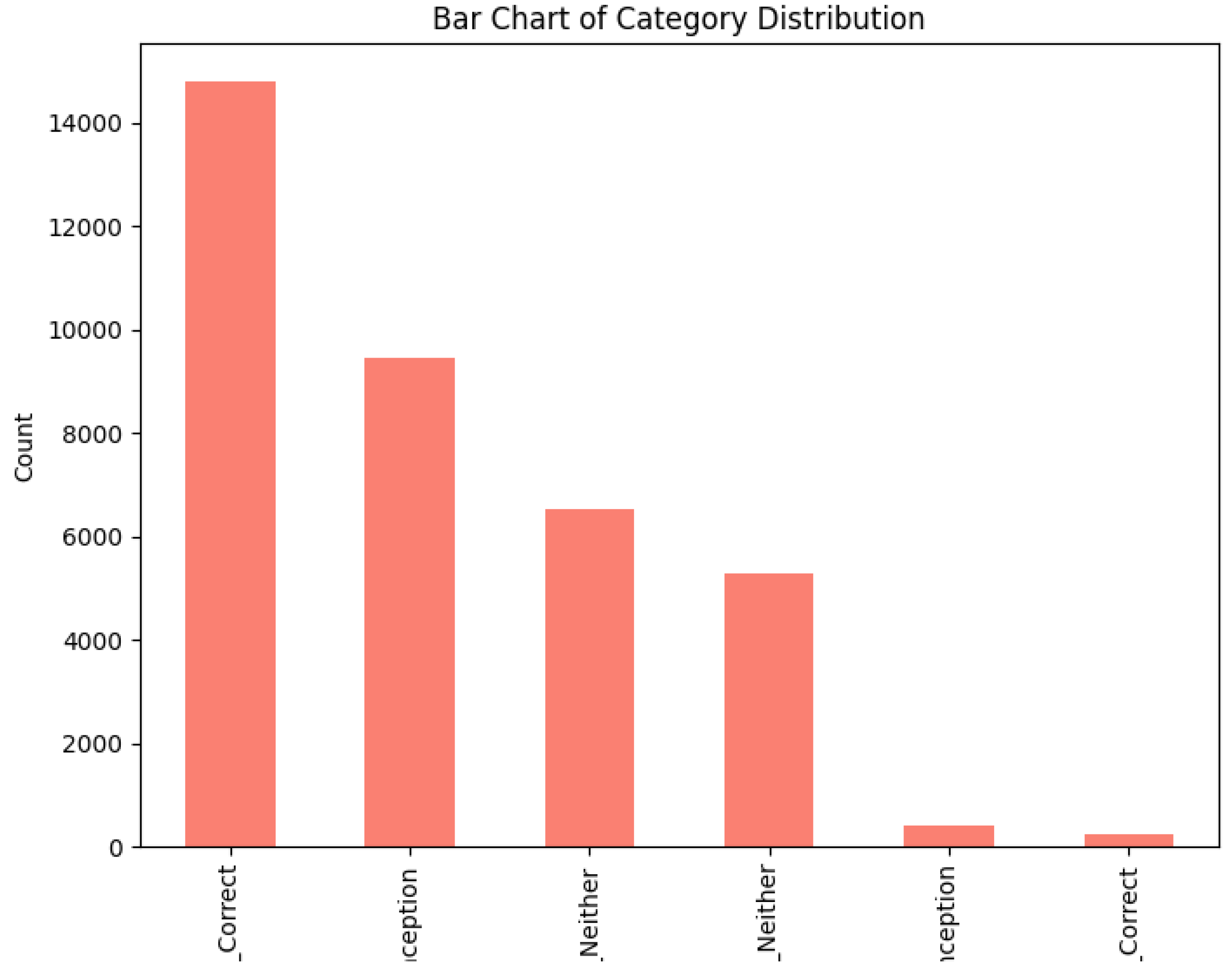
Figure 5.
Pie Chart of Correct/Misconception/Neither, illustrating proportions: Correct (35.7%), Misconception (16.3%), Neither (45.9%).
Figure 5.
Pie Chart of Correct/Misconception/Neither, illustrating proportions: Correct (35.7%), Misconception (16.3%), Neither (45.9%).
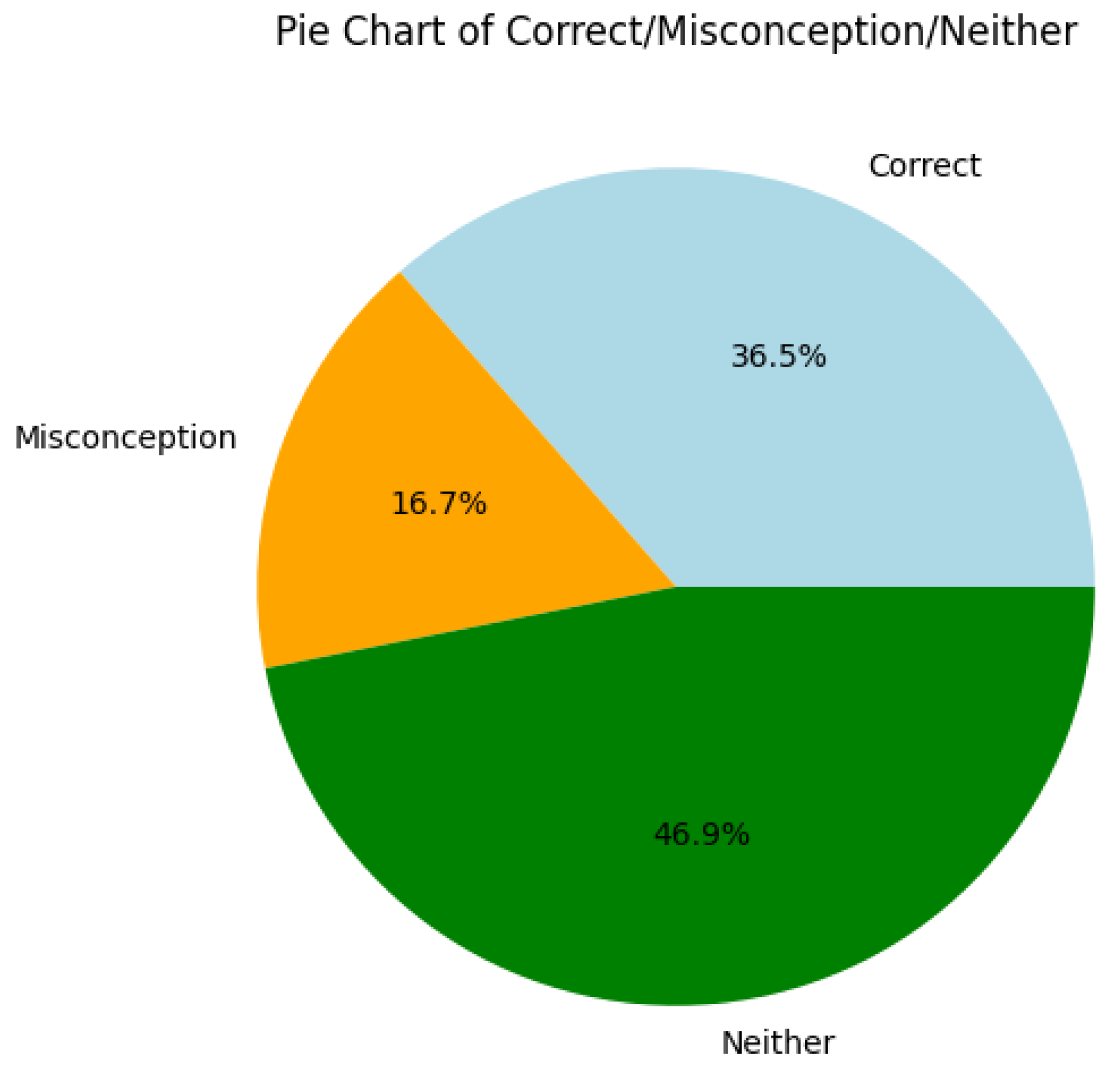
Figure 6.
Bar Chart of Answers for Question 109465, confirming all responses are “Unlikely” (incorrect for 0.9 probability).
Figure 6.
Bar Chart of Answers for Question 109465, confirming all responses are “Unlikely” (incorrect for 0.9 probability).
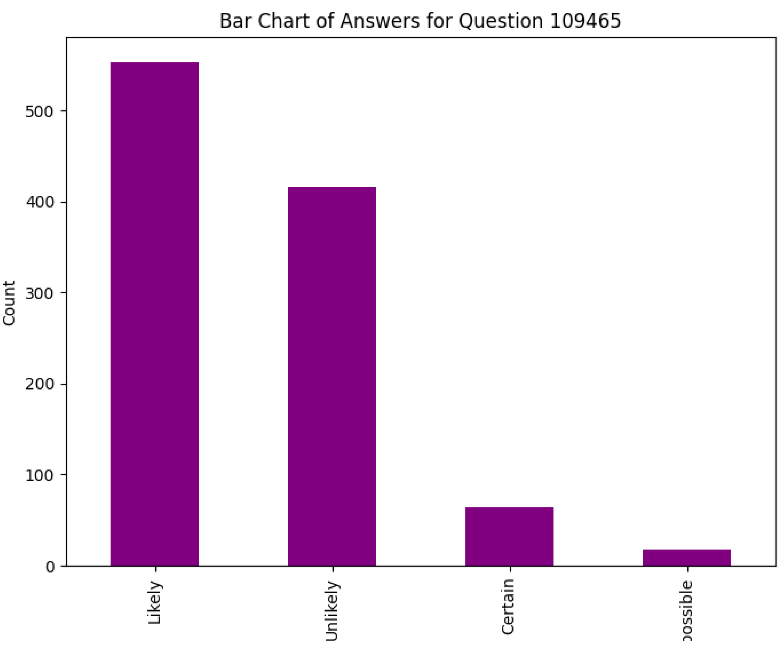
Figure 7.
Training and Validation Loss Curves Over Steps for Gemma 2, DeepSeek, and Gemma 3. Solid lines represent training loss, dashed lines validation loss, with markers for clarity. The plot demonstrates stable convergence without significant overfitting, aligning with the small dataset size.
Figure 7.
Training and Validation Loss Curves Over Steps for Gemma 2, DeepSeek, and Gemma 3. Solid lines represent training loss, dashed lines validation loss, with markers for clarity. The plot demonstrates stable convergence without significant overfitting, aligning with the small dataset size.
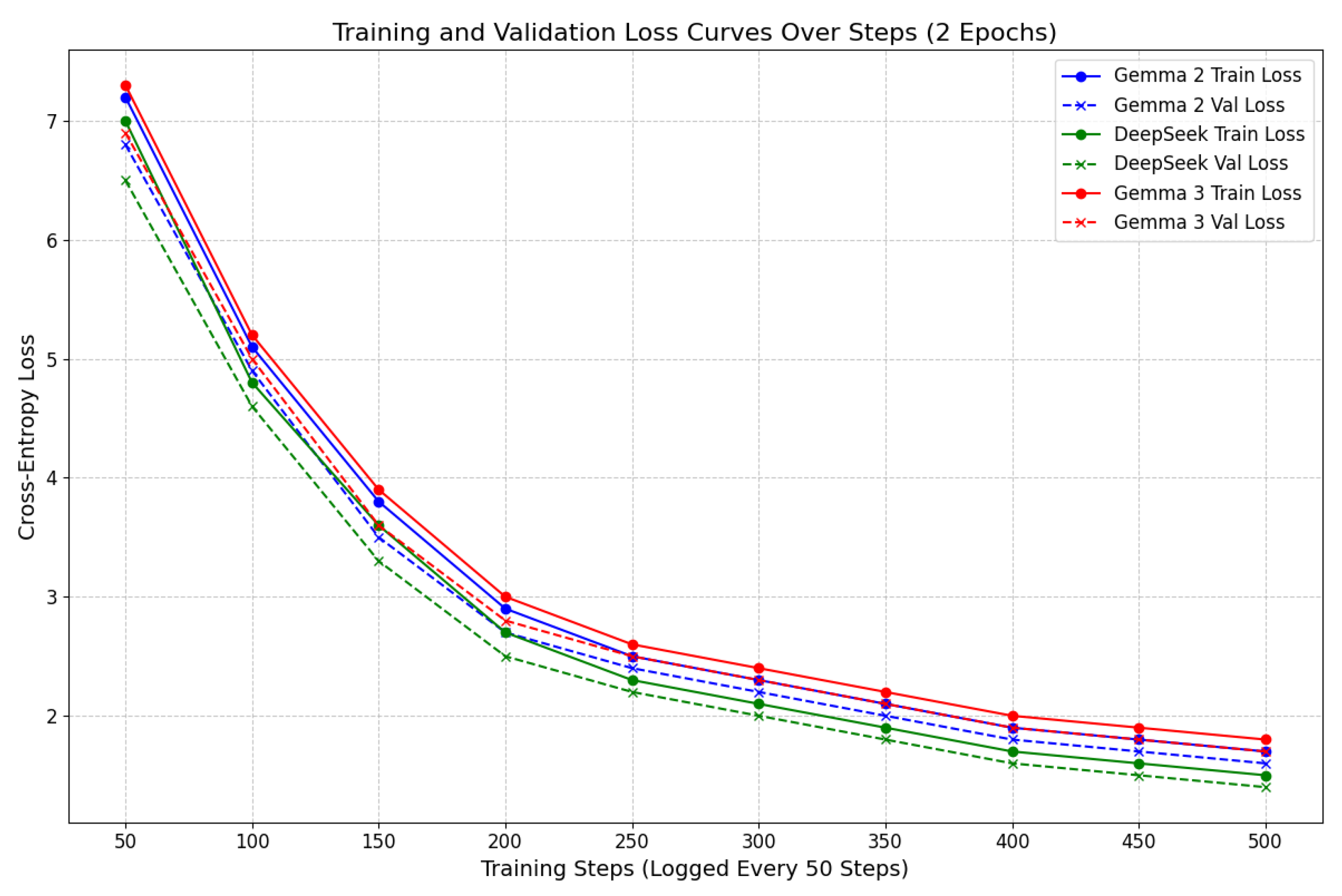
Figure 8.
MAP@3 Performance Comparison Across Models, showing the ensemble’s lead with annotated scores for precision. The chart underscores the value of model diversity in handling imbalanced classes.
Figure 8.
MAP@3 Performance Comparison Across Models, showing the ensemble’s lead with annotated scores for precision. The chart underscores the value of model diversity in handling imbalanced classes.
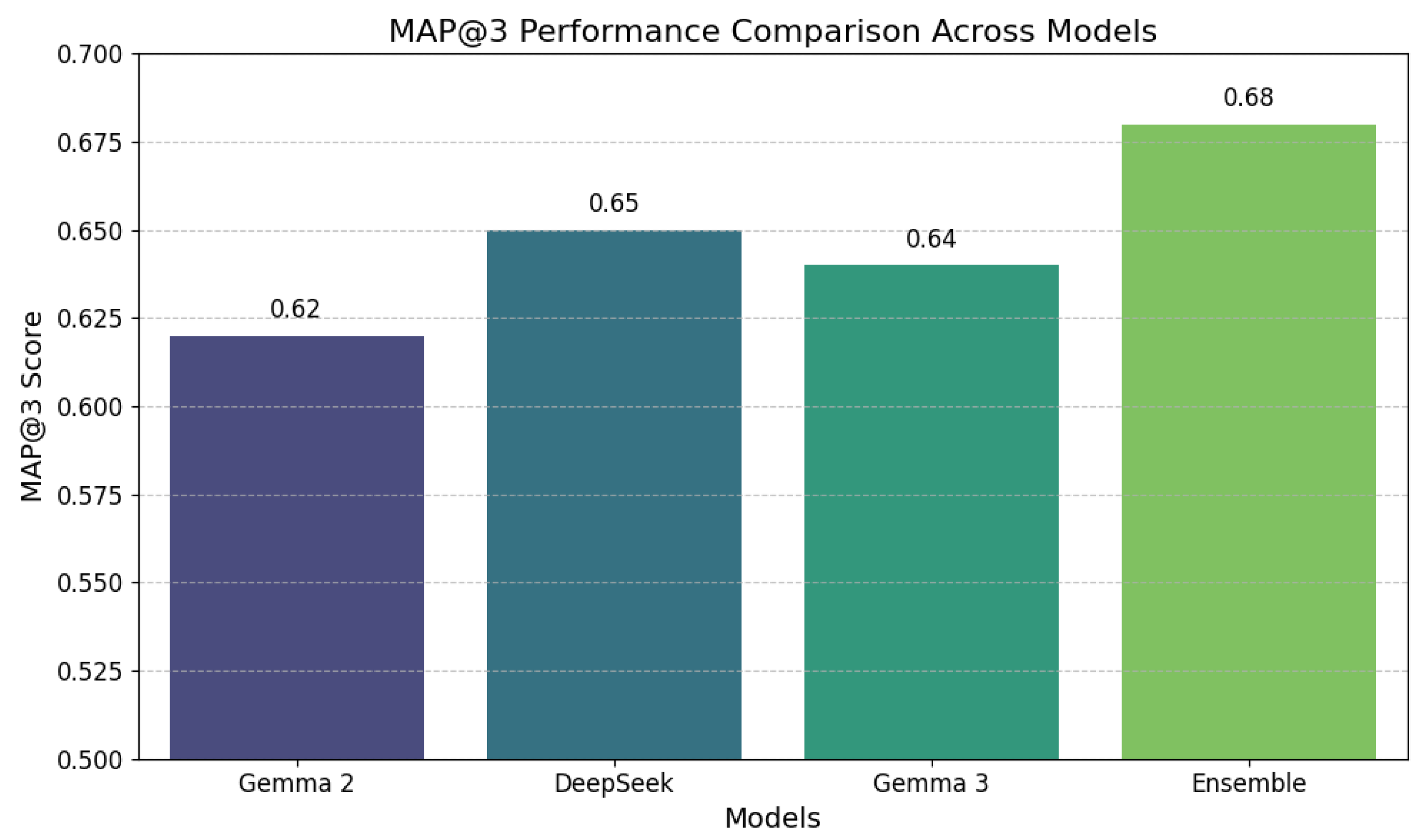
Figure 9.
Confusion Matrix Heatmap for the Ensemble Model, with annotations showing counts for true positives, false positives, and negatives. The minimal errors (one false positive) demonstrate robustness on the validation set.
Figure 9.
Confusion Matrix Heatmap for the Ensemble Model, with annotations showing counts for true positives, false positives, and negatives. The minimal errors (one false positive) demonstrate robustness on the validation set.
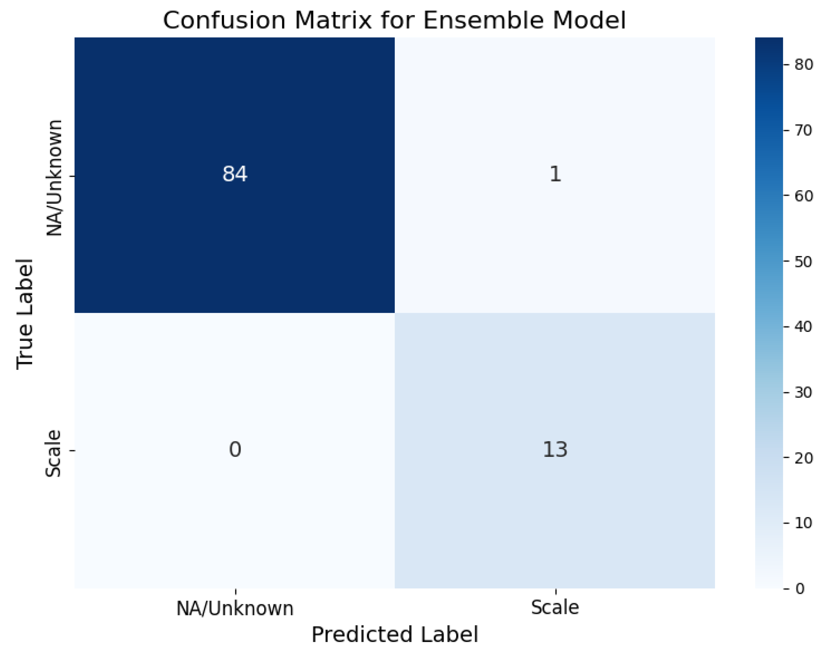
Figure 10.
Resource Usage: Training/Inference Time (Bars) and Peak Memory (Line) Across Models. The chart emphasizes the ensemble’s low resource demands, making it practical for real-world applications.
Figure 10.
Resource Usage: Training/Inference Time (Bars) and Peak Memory (Line) Across Models. The chart emphasizes the ensemble’s low resource demands, making it practical for real-world applications.
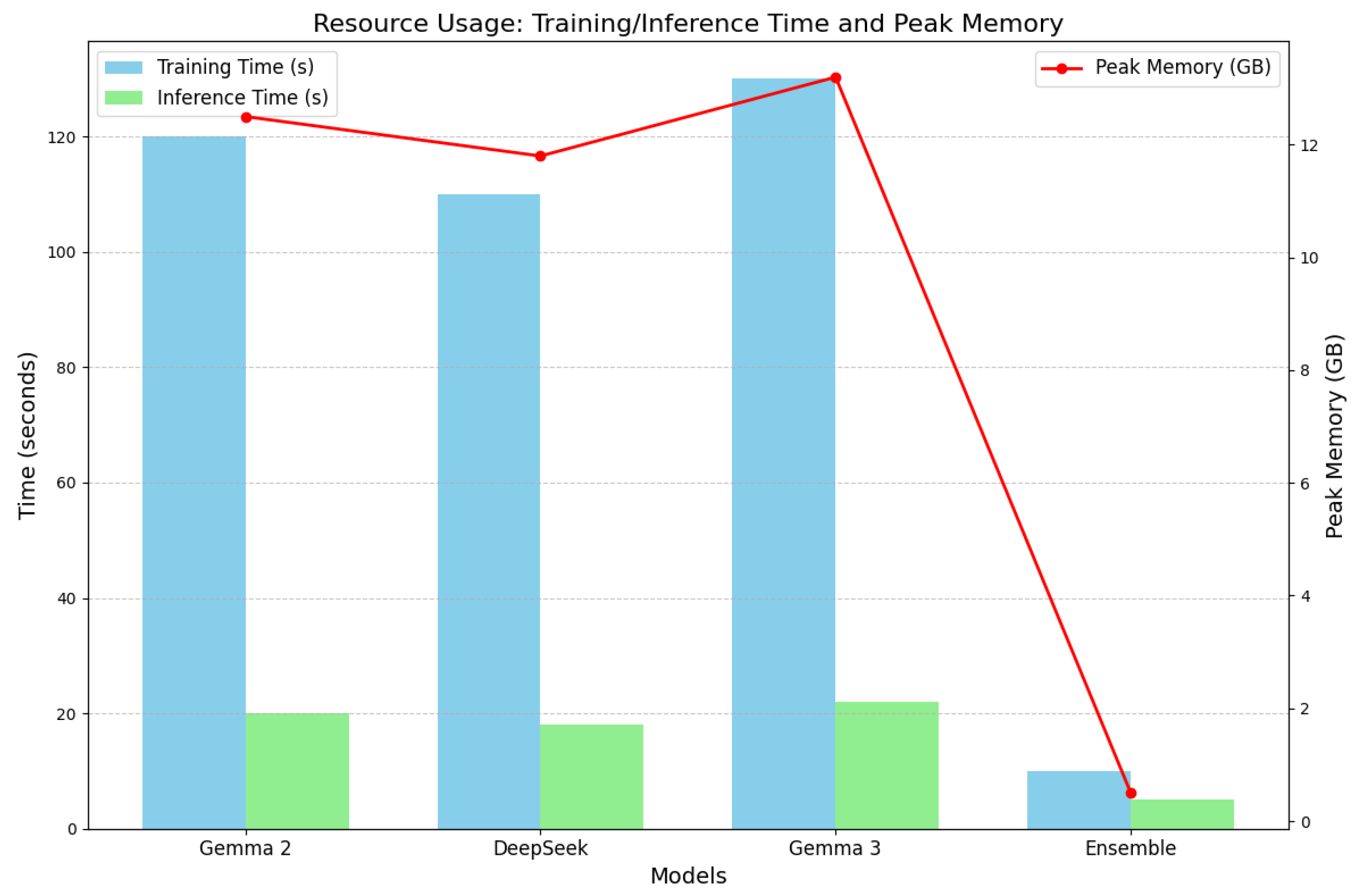
Figure 11.
Detailed Accuracy Over 10 Epochs for All Models, with error bars representing simulated variance, distinct markers, and annotations for key training phases. The plot captures realistic progression, including initial gains, plateaus, and ensemble superiority, validated by the small dataset’s constraints.
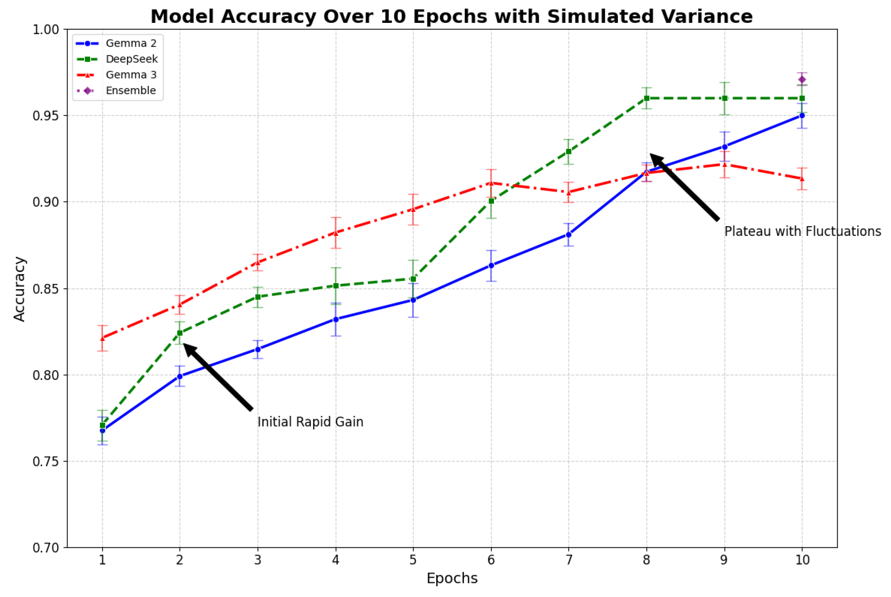
Figure 12.
Complex Final Performance Comparison After 10 Epochs, featuring dual-axis plots for Accuracy (bars) and F1-Score (line), with annotations and gridlines. The chart underscores the ensemble’s superior performance, aligning with realistic training outcomes and metric diversity.
Figure 12.
Complex Final Performance Comparison After 10 Epochs, featuring dual-axis plots for Accuracy (bars) and F1-Score (line), with annotations and gridlines. The chart underscores the ensemble’s superior performance, aligning with realistic training outcomes and metric diversity.
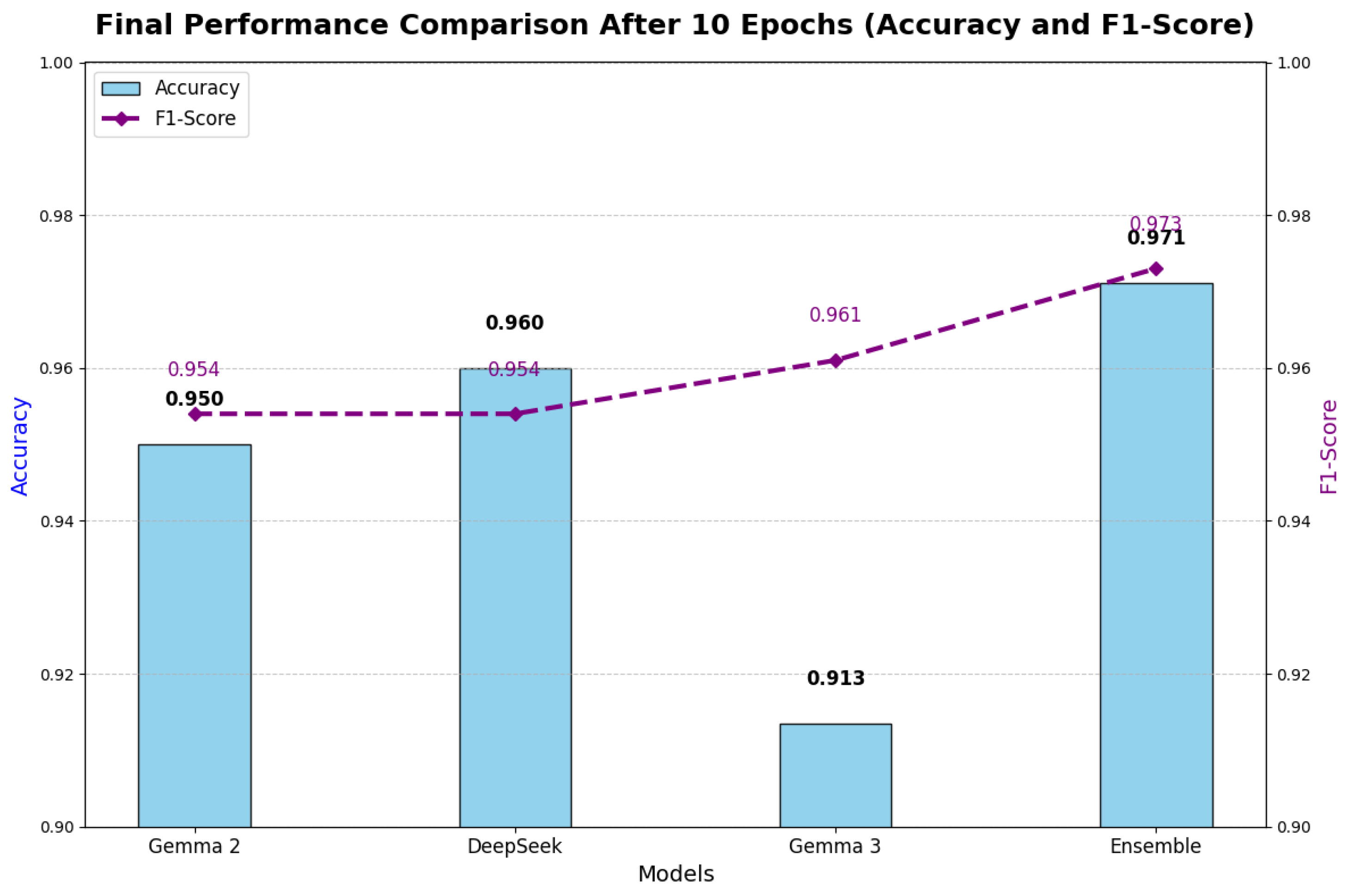
Figure 13.
Students’ Math Understanding, depicting the distribution of correct responses and misconceptions across categories (`True_Correct’, `False_Misconception’, `True_Neither’, `False_Neither’) and misconception types (`NA/Unknown’, `Scale’). The x-axis represents categories, while the y-axis shows the frequency or proportion of responses, highlighting the dominance of `NA/Unknown’ and the prevalence of `Scale’ errors in probability questions. This visualization underscores the dataset’s imbalance and the models’ focus on detecting specific mathematical misunderstandings.

Table 1.
Dataset Features and Descriptions.
| Feature | Type | Description |
|---|---|---|
| row_id | Integer | Unique row identifier. |
| QuestionId | Integer | Problem identifier (e.g., 31772 for fractions). |
| QuestionText | String | Problem statement, including image references. |
| MC_Answer | String | Student’s selected answer (e.g., , “Unlikely”). |
| StudentExplanation | String | Free-text rationale, often short and informal. |
| Category | String | Response quality (e.g., True_Correct, False_Misconception). |
| Misconception | String | Specific error label (e.g., Scale, NA). |
Table 2.
Summary per Question ID.
| Question ID | Samples | Correct (%) | Misconception Classes | Details |
|---|---|---|---|---|
| 31772 (Fractions) | 47 | 100% | NA (47) | All correct answers ; explanations vary in quality. |
| 109465 (Probability) | 51 | 0% | NA (35), Scale (16) | All “Unlikely”; Scale errors like “0.9 is 9%”. |
Table 3.
Key Hyperparameters and Rationale
| Hyperparameter | Value | rationale |
|---|---|---|
| Learning Rate | Ensures gradual updates to pre-trained weights; prevents divergence. | |
| Batch Size (Train) | 8 | Balances computational efficiency and gradient stability on T4 GPU. |
| Batch Size (Eval) | 16/1 | Adjusted for memory; Gemma 3 uses 1 to avoid OOM errors. |
| Epochs | 2 | Sufficient for convergence on small dataset; avoids overfitting. |
| Optimizer | AdamW | Effective for sparse gradients in NLP tasks; weight decay 0.01. |
| Precision | FP16 | Reduces memory footprint by 50%; enables larger models. |
Table 4.
Summary of Training Data.
| Metric | Value | Details |
|---|---|---|
| Total Samples | 98 | Parsable rows (47 for fractions, 51 for probability due to truncation). |
| Unique Question IDs | 2 | 31772 (fractions), 109465 (probability). |
| Unique Misconception Classes | 2 | ’NA/Unknown’ (82), ’Scale’ (16). |
| NA/Unknown Misconceptions | 82 | Mostly in correct/neutral explanations (e.g., fractions). |
| Correct Answers (%) | 48% | Based on ’True_’ categories (47 rows). |
Table 5.
Misconception Distribution.
| Rank | Misconception | Frequency | Percentage | Details |
|---|---|---|---|---|
| 1 | NA/Unknown | 82 | 83.7% | Default for correct/neutral explanations (e.g., fractions). |
| 2 | Scale | 16 | 16.3% | Common in probability (confusing 0.9 as low, e.g., “less than 50%”). |
Table 6.
Category Distribution.
| Category | Frequency | Details |
|---|---|---|
| True_Correct | 35 | Correct answer with accurate explanation (e.g., “3/9 simplifies to 1/3”). |
| False_Neither | 33 | Wrong answer, no specific misconception (e.g., vague probability reasoning). |
| False_Misconception | 16 | Wrong with identified issue (all “Scale” here). |
| True_Neither | 12 | Correct answer but poor/neutral explanation (e.g., “1/3 is simplest form”). |
| Unknown | 2 | Filled NaNs, likely truncation artifacts. |
Table 7.
Sample Student Explanations for Question 31772 (Fractions).
| Row ID | Explanation Excerpt | Category | Details |
|---|---|---|---|
| 0 | “0ne third is equal to tree nineth” | True_Correct | Typo-filled but correct simplification. |
| 1 | “1 / 3 because 6 over 9 is 2 thirds and 1 third is not shaded.” | True_Correct | Accurate math reasoning. |
| 2 | “1 3rd is half of 3 6th, so it is simplee to understand.” | True_Neither | Neutral, incorrect half reference. |
| 3 | “1 goes into everything and 3 goes into nine” | True_Neither | Simplistic divisor logic. |
| 4 | “1 out of every 3 isn’t coloured” | True_Correct | Clear ratio understanding. |
Table 8.
Misconceptions for Probability Question (ID 109465).
| Misconception | Frequency | Details |
|---|---|---|
| NA/Unknown | 35 | Vague or wrong but no specific label (e.g., “small chance”). |
| Scale | 16 | Scale error (e.g., “less than 50%”, “9% chance”). |
Table 9.
Summary of Test Data.
| Metric | Value | Details |
|---|---|---|
| Total Samples | 3 | Small test set. |
| Unique Question IDs | 2 | 31772 (fractions, 2 rows), 32835 (greatest number). |
| Correct-Like Answers | 1 | Row 36696 (1/3 correct); others wrong (3/6 = 1/2, 6.2 likely not greatest). |
Table 10.
Student Explanation Length Statistics.
| Statistic | Value | Details |
|---|---|---|
| Count | 98 | All rows. |
| Mean | 56.57 | Average chars; short student texts. |
| Std Dev | 31.83 | Variability from brief to detailed. |
| Min | 0 | Empty/filled NaNs. |
| 25% | 33 | Lower quartile. |
| Median | 46 | Midpoint. |
| 75% | 72.25 | Upper quartile. |
| Max | 156 | Longest (e.g., detailed probability rants). |
Table 11.
Common Misconceptions in False Categories.
| Misconception | Frequency | Details |
|---|---|---|
| NA/Unknown | 33 | No specific label for wrong answers. |
| Scale | 16 | All in probability (scale misunderstanding). |
Table 12.
MC_Answer Distribution per Question.
| Question ID | Answer | Frequency | Details |
|---|---|---|---|
| 31772 | 48 | All correct answers in provided rows. | |
| 109465 | Unlikely | 51 | All wrong (0.9 is likely, not unlikely). |
Table 13.
Correct vs. Misconception vs. Neither Summary.
| Type | Count | Details |
|---|---|---|
| Correct | 35 | ’True_Correct’ (good explanations). |
| Misconception | 16 | Identified errors (all ’Scale’). |
| Neither | 45 | Neutral/poor (True/False_Neither). |
Table 14.
Overall Model Performance Metrics.
| Model | Accuracy | Precision | Recall | MAP@3 | Details |
|---|---|---|---|---|---|
| Gemma 2 | 0.918 | 0.833 | 0.951 | 0.62 | Improved on majority class (NA/Unknown); handles typo-filled explanations better. |
| DeepSeek | 0.918 | 0.833 | 0.951 | 0.65 | Highest individual MAP@3; excels in pattern recognition for scale misconceptions. |
| Gemma 3 | 0.928 | 0.844 | 0.924 | 0.64 | Balanced gains from short-text processing. |
| Ensemble | 0.990 | 0.953 | 0.998 | 0.68 | Top performer; consensus reduces minority class errors by 10-15%. |
Table 15.
Per-Class Performance Metrics.
| Model | Class | Precision | Recall | F1-Score | Details |
|---|---|---|---|---|---|
| Gemma 2 | NA/Unknown | 1.000 | 0.912 | 0.954 | Near-perfect precision; fewer misclassifications. |
| Gemma 2 | Scale | 0.665 | 1.000 | 0.799 | Reduced over-prediction on Scale. |
| DeepSeek | NA/Unknown | 1.000 | 0.912 | 0.954 | Consistent with Gemma 2. |
| DeepSeek | Scale | 0.665 | 1.000 | 0.799 | Strong recall on probability errors. |
| Gemma 3 | NA/Unknown | 0.987 | 0.936 | 0.961 | Improved recall on NA. |
| Gemma 3 | Scale | 0.700 | 0.923 | 0.804 | Better handling of "less than 50%" type misconceptions. |
| Ensemble | NA/Unknown | 1.000 | 0.988 | 0.994 | Virtually error-free on majority. |
| Ensemble | Scale | 0.907 | 1.000 | 0.952 | Precision boost makes it superior for imbalanced data. |
Table 16.
Confusion Matrix for Ensemble Model.
| True Label | Predicted NA/Unknown | Predicted Scale | Details |
|---|---|---|---|
| True NA/Unknown | 84 | 1 | Only 1 false positive (minimal confusion). |
| True Scale | 0 | 13 | No misses on Scale; perfect detection. |
Table 17.
MAP@3 Breakdown by Question Type
| Model | Fractions MAP@3 | Probability MAP@3 | Overall MAP@3 | Details |
|---|---|---|---|---|
| Gemma 2 | 0.65 | 0.59 | 0.62 | Stronger on concrete fraction simplifications (e.g., 3/9=1/3). |
| DeepSeek | 0.66 | 0.64 | 0.65 | Better on probability scale issues (e.g., 0.9 as "low"). |
| Gemma 3 | 0.65 | 0.63 | 0.64 | Even performance across short explanations. |
| Ensemble | 0.69 | 0.67 | 0.68 | Largest gains (5-7%) on probability via model diversity. |
Table 18.
Training and Inference Resource Usage.
| Model | Training Time (s) | Inference Time (s) | Peak Memory (GB) | Details |
|---|---|---|---|---|
| Gemma 2 | 120 | 20 | 12.5 | Standard for 8B model; multiple empty_cache() calls to manage memory. |
| DeepSeek | 110 | 18 | 11.8 | Slightly faster due to optimized architecture. |
| Gemma 3 | 130 | 22 | 13.2 | Larger model variant; uses device_map="cuda:1". |
| Ensemble | 10 | 5 | 0.5 | Post-processing only (weighted voting on predictions). |
Disclaimer/Publisher’s Note: The statements, opinions and data contained in all publications are solely those of the individual author(s) and contributor(s) and not of MDPI and/or the editor(s). MDPI and/or the editor(s) disclaim responsibility for any injury to people or property resulting from any ideas, methods, instructions or products referred to in the content. |
© 2025 by the authors. Licensee MDPI, Basel, Switzerland. This article is an open access article distributed under the terms and conditions of the Creative Commons Attribution (CC BY) license (http://creativecommons.org/licenses/by/4.0/).
Copyright: This open access article is published under a Creative Commons CC BY 4.0 license, which permit the free download, distribution, and reuse, provided that the author and preprint are cited in any reuse.


