
Submitted:
02 October 2025
Posted:
02 October 2025
You are already at the latest version
Abstract
This paper proposes a multi-objective optimization method that integrates deep neural networks (DNN) with grey relational analysis (GRA) to optimize lay-up configurations for carbon fiber-reinforced plastic (CFRP) automotive components. Specifically, a lab-scale CFRP B-pillar structure was investigated to simultaneously maximize structural strength and failure safety. A DNN surrogate model was trained using finite element simulations of 2,000 random stacking sequences to achieve high predictive accuracy. The trained model was then used to evaluate all possible lay-up combinations to derive Pareto optimal solutions. Grey relational analysis was subsequently employed to select the final optimal configurations based on designer preferences. The selected lay-up designs demonstrated improvements in both strength and failure safety. To validate the proposed framework, laboratory-scale CFRP B-pillar was fabricated using a prepreg compression molding process and subjected to bending tests. The experimental results confirmed an error below 5% and failure trends consistent with the simulation results, thereby validating the reliability of the proposed method. The proposed DNN-GRA approach enables efficient multi-objective optimization with reduced computational effort and flexibility in reflecting different engineering priorities.
Keywords:
carbon fiber reinforcement plastic (CFRP)
; deep neural networks (DNN)
; pareto optimal solutions
; grey relational analysis(GRA)
; multi-objective optimization
1. Introduction
The automotive industry has increasingly focused on improving vehicle safety and reducing environmental impacts through lightweight structural designs. Among the various lightweight materials, carbon fiber-reinforced plastics (CFRP) are suitable for addressing this problem because of their superior specific strength, stiffness, and excellent fatigue performance compared to conventional metallic materials. Therefore, CFRP has been widely applied in structural components, particularly in safety-critical parts such as the B-pillar of vehicle. However, the effective design of CFRP structures remains challenging, particularly when multiple performance objectives, such as strength and crashworthiness, must be simultaneously optimized.The growing demand for CO2 reduction has accelerated the development of hybrid and electric vehicles utilizing lightweight components [1]. In particular, extensive research has been conducted to replace traditional steel components with CFRP owing to its high strength and stiffness. Liu et al. developed a lightweight CFRP frame for electric vehicles [2], whereas Wang et al. applied CFRP to the design of automotive wheel rims to achieve a significant weight reduction compared with conventional materials [3]. The mechanical performance of CFRP structures is highly influenced by design variables, such as thickness [4], stacking angle [5], and lay-up sequence [6]. Accordingly, various optimization strategies have been applied to derive the optimal lay-up configurations. Owing to the nonlinear and complex relationship between design variables and mechanical properties, advanced surrogate modeling techniques have been increasingly utilized. Lee et al. performed thickness and lay-up optimization of CFRP-reinforced B-pillars using a genetic algorithm (GA) to maximize the bending stiffness [7]. Similarly, Shrivastava et al. optimized the stacking sequence of a double-double (DD) laminate for aerospace wing applications using an artificial intelligence (AI)-enhanced GA approach [8]. Moreover, Serban et al. applied various machine learning algorithms to predict fracture behavior based on CFRP lay-up configurations [9].
Engineering design problems typically involve multiple objectives and constraints that often conflict. For example, when the stacking sequence of a CFRP component is optimized with respect to strength alone, the fracture resistance can be inadvertently compromised. Thus, a multi-objective optimization approach is essential to simultaneously enhance multiple performance criteria. Recently, the Taguchi method combined with grey relational analysis (GRA) has been widely used for efficient multi-objective optimization with a reduced number of experiments. Shunmugesh et al. applied the Taguchi-GRA method to optimize microdrilling parameters for CFRP, confirming the influence of the material feed rate and spindle speed using an analysis of variance (ANOVA) [10]. However, the Taguchi method does not fully account for the interactions among the design variables, and its performance can vary depending on the selected experimental design, often leading to convergence toward local optima [11]. Sebaey et al. applied ant colony optimization (ACO) to obtain the optimal stacking sequences of CFRP laminates under low-velocity impact conditions [12]. Their study demonstrated a 21% reduction in the damaged area and an 8% improvement in the delamination threshold load compared with the base configuration. Although ACO shows strong performance in solving discrete optimization problems and offers stable results, it suffers from relatively slow convergence rates and lower solution precision [13]. Multi-objective genetic algorithms (MOGA) extend the capabilities of GA by applying Pareto optimality concepts to multi-objective problems. Beylergil et al. employed the MOGA to optimize the stacking sequence of CFRP plates subjected to eccentric loading [14]. The optimized configurations achieved improvements of 7% and 12% in strength and safety factors, respectively, compared with the base design. Although the MOGA effectively finds high-quality solutions in discrete spaces, it is computationally expensive and requires considerable time for convergence [15].
Therefore, a methodology is required to account for the interactions among global design variables, such as deep neural networks (DNNs), to minimize computational time while maintaining optimization quality. The integration of Pareto optimality-based algorithms further enables the derivation of high-quality multi-objective solutions. In this study, a multi-objective optimization approach combining a DNN surrogate model with GRA is proposed to efficiently derive high-quality Pareto optimal solutions with reduced computational effort. The proposed approach was applied to the multi-objective lay-up optimization of a lab-scale CFRP B-pillar to simultaneously enhance strength and failure safety. Finally, to validate the proposed DNN-GRA optimization approach, a lab-scale CFRP B-pillar was fabricated using a prepreg compression molding (PCM) process, and the bending test was performed under the same conditions as the finite element analysis (FEA).
2. Method of Multi-Objective Optimization
The procedure for the proposed multi-objective optimization methodology for the CFRP lay-up design, which integrates the DNN surrogate model and GRA, is illustrated in Figure 1. The overall process consists of three main stages: (a) construction of a DNN surrogate model based on training data through FEA, (b) generation of the solution space and extraction of the Pareto optimal set, and (c) selection of the optimal solution using GRA, according to the designer’s preferences.
First, to train the DNN surrogate model, a set of simulation data is generated using finite element analysis (Generate training data using FEA). The number of samples was determined based on the complexities and dimensions of the design variables. The FEA results were then normalized to a range between zero and one to enhance the learning performance of the DNN (Preprocessing the training data). Hyperparameter tuning was performed to determine the optimal DNN architecture (Hyperparameter optimization and training of the DNN model). The model with the best predictive performance on the validation set was saved for subsequent analysis (Save DNN model).
Second, the trained DNN model is used to predict the values of the objective function for all possible combinations of design variables (All possible cases of design variables are predicted using the DNN model). A one-to-one mapping of the predicted values was employed to generate the solution space (Generate solution space using the predicted data). From this solution space, the Pareto optimal set is extracted using a non-dominated sorting approach (Obtain the Pareto optimal set from the solution space using non-dominated point sorting).
Finally, to identify the most suitable solution according to the designer’s preferences, the GRA was applied to the previously derived Pareto optimal set. This involves several steps: (a) normalization of each objective function based on whether it follows the larger-the-better, smaller-the-better, or nominal-the-best characteristics (Normalized objective values of the Pareto optimal set), (b) calculation of the absolute difference between the reference and normalized values to determine the grey relational coefficient (GRC), (c) computation of the GRC for each Pareto solution, and (d) derivation of the grey relational grade (GRG) by applying weight factors to each objective function. The solution with the highest GRG value is selected as the optimal solution.
2.1. DNN Surrogate Model
Deep neural networks (DNNs), a class of artificial neural networks (ANNs) with multiple hidden layers, are machine learning models characterized by high adaptability, self-organization, and self-learning capabilities. These models are particularly well-suited for approximating complex nonlinear relationships between inputs and outputs, even when the training data are limited or noisy [16]. DNNs operate using interconnected layers of perceptron, where the output of each node is computed using Equation (1) [17]:
where Yj is the output of node j; f is the activation function; n is the number of nodes; Yi is the output of node i; wij is the connection weight; and bj is the bias term of node j.
Traditional activation functions such as sigmoid and hyperbolic tangents are widely used in backpropagation learning processes. However, as the network depth increases, these functions often suffer from the gradient vanishing problem, where the gradients become too small for effective learning [18]. To overcome this problem, the rectified linear unit (ReLU) activation function shown in Equation (2) was adopted for deeper architectures [19].
The ReLU function outputs zero for negative inputs and a linear response for positive inputs, thereby accelerating the training process and alleviating the vanishing gradient problem. In this study, the DNN was trained using an adaptive moment estimation (Adam) optimizer, which has demonstrated robust performance in navigating parameter spaces and has been widely adopted for DNN training tasks [20]. A schematic of the constructed deep neural network architecture is shown in Figure 2. The model comprises an input layer, several hidden layers, and two output nodes corresponding to the maximum load and margin of safety (MoS). ReLU activation was applied to each hidden layer, and the Adam optimizer was used for model training. Early stopping was implemented to prevent overfitting during the training. To assess the prediction accuracy of the trained model, three standard evaluation criteria were used: the Mean Absolute Error (MAE), Root Mean Square Error (RMSE), and coefficient of determination (R2). The definitions of these metrics are
where n is the number of input data, ŷ is the predicted value, y is the actual value, and ȳ is the mean of the actual values. MAE quantifies the average magnitude of prediction errors and is less sensitive to outliers. RMSE, which squares the residual before averaging, penalizes larger errors more strongly, making it particularly sensitive to the impact of extreme deviations. R2 measures the proportion of variance in the dependent variable that can be predicted from the independent variables. Values of R2 closer to 1 indicate better model performance.
2.2. Pareto Optimal Set
Pareto optimality is a widely used concept in multi-objective optimization that acknowledges that the improvement of one objective function often leads to the degradation of another. In such scenarios, the goal is not to find a single global optimum but rather to identify a set of trade-off solutions that are non-dominated with respect to each other. This set is referred to as the Pareto optimal set [21].
Mathematically, let Ω denote the feasible region in the objective space, and let x ∈ X represent a point in the decision space. The image of x under the objective function vector is denoted as z = f(x) ∈ Ω. The objective of Pareto optimization is to extract the set of non-dominated solutions from the feasible region defined by Equation (6) and illustrated in Figure 3:
Here, a solution x(1) is said to dominate another solution x(2) denoted as x(1) ≺ x(2), if the following two conditions are met [22]:
Condition 1 (Non-worseness):
Condition 2 (Strict improvement in at least one objective):
A solution is considered non-dominated if no other solution in the feasible space satisfies both of these conditions. All non-dominated solutions collectively form the Pareto optimal set, which characterizes the boundary of the achievable trade-offs. The process of identifying the Pareto optimal set through non-dominated sorting is illustrated in Figure 4. In this process, the candidate solution j from the solution space is compared with every other solution i. If i dominates j, then j is removed from the candidate set P′. If j is not dominated by any solution i, it remains in P′. This iterative comparison is performed for all i ∈ {1, 2, …, N}, where N is the total number of feasible solutions. The final set P′ after completing all comparisons constitutes the Pareto optimal set.
The Pareto set obtained in this study represents a set of feasible CFRP lay-up configurations that simultaneously consider the trade-offs between the maximum structural strength and failure safety, which are considered as multi-objective functions. This set is used as the input for the subsequent decision-making phase using the GRA, where the most preferred solution is selected based on the designer’s specified weights.
2.3. Grey Relational Analysis
In this study, GRA was employed to select a single optimal solution from the Pareto optimal set, reflecting the designer’s specified weighting of the objectives. The decision-making process followed the structured four-step procedure detailed below [23]:
Step 1: Normalization of Pareto optimal values
The values predicted in the Pareto optimal solution were normalized based on the following objective characteristics: larger-the-better (LTB), smaller-the-better (STB), or nominal-the-best (NTB). The normalized value xi∗ (k) for the ith solution and the kth objective function was calculated as:
where xi(k) is the original value of the kth objective for the ith solution, and T is the target value for the NTB objectives. In this study, both objectives followed the LTB characteristics.
Step 2: Calculation of absolute deviation from reference
To evaluate the proximity of each normalized value to the ideal value, the absolute deviation from the reference value (assumed to be 1) was calculated as follows:
where x0∗(k) = 1 is the reference (ideal) normalized value.
Step 3: Computation of grey relational coefficient (GRC)
The grey relational coefficient for each objective function was computed using:
where Δmin and Δmax are the minimum and maximum of all Δ0i(k), and ∈ [0, 1] is the distinguishing coefficient (typically set to 0.5).
Step 4: Computation of grey relational grade (GRG)
The overall performance of each solution was evaluated by the grey relational grade , calculated as a weighted sum of the GRCs:
where wk denotes the weight assigned to the kth objective function. The weights reflect the designer priorities and satisfy the following constraints:
In this study, the proposed DNN-GRA methodology was applied to the multi-objective optimization of lay-up configurations for a lab-scale CFRP B-pillar. Two objective functions were defined to maximize the structural strength and failure safety under bending deformation. Both objectives were defined with a larger-the-better (LTB) characteristic, and GRA was performed using the corresponding normalization method. Specifically, normalized objective values were used to calculate the GRCs, which were then aggregated into a GRG through weighted summation. The solution with the highest GRG value was selected as the optimal final configuration. This approach enables an efficient optimal lay-up design that simultaneously satisfies both mechanical performance targets.
3. Results
3.1. Problem Definition and Design Variables
The target structure for optimization in this study was a lab-scale CFRP B-pillar, which was modeled using CATIA V5 based on the geometry of typical automotive B-pillar components, as shown in Figure 5. For comparative evaluation with conventional steel body panels, a woven thermoset CFRP prepreg from TORAY was selected as the material for the lab-scale CFRP B-pillar. Six CFRP prepreg layers of 0.2 mm thickness per ply were stacked to achieve the same thickness as a DP590 steel panel of 1.2 mm thickness. The design variables used in this study were the fiber orientation angles of the six prepreg plies. Based on the feasible manufacturing and orthotropic behavior of the woven composites, the allowable ply angles were discretized in 15° increments as follows:
The total number of combinations of design variables was 66 (=46,656), representing all possible lay-up configurations within the specified angle set. Two objective functions were defined to maximize the structural strength and failure safety simultaneously. Specifically, two criteria were evaluated at a prescribed deformation level corresponding to a punch stroke of 14 mm: (a) maximum load (structural strength) and (b) maximum failure safety (MoS), which were calculated using the modified Tsai-Wu failure criterion. The Tsai-Wu failure criterion was employed to evaluate the failure behavior of each lay-up configuration under bending. This strength-based failure model considers the combined effects of in-plane stresses and provides a scalar failure index (FI), which is calculated as follows:
Expanded into in-plane components, the equation becomes:
The corresponding strength tensors, Fi and Fij are defined using the tensile, compressive, and shear strengths of the material as follows:
where Xt, Xc, Yt, and Yc are the tensile and compressive strengths in the fiber and transverse directions, respectively, and S is the in-plane shear strength. The material properties of the CFRP are listed in Table 1. Table 2 lists the strength values obtained from the technical datasheet of the manufacturer.
Although the Tsai–Wu index (FI = 1) identifies the onset of failure, it does not provide a quantitative measure of safety margin when FI<1 [24,25]. To address this, a safety factor R was introduced as the ratio of the allowable stress to the actual stress, enabling a continuous measure of structural reliability [26]:
Substituting this relationship into the Tsai-Wu expression yields a quadratic equation in terms of R:
Where the coefficients a and b are defined as:
Solving the quadratic yields the safety factor:
Finally, the margin of safety (MoS) is defined as the surplus capacity beyond the applied load, given by:
This metric offers intuitive insight: for instance, MoS=1 indicates that the structure can withstand twice the applied load, while MoS=−0.5 implies failure unless the load is reduced by at least 50%.
The deformation condition used in this study was based on the mechanical characteristics of automotive body panels with 1.2 mm-thick steel sheets, which generally exhibit elastic load responses up to 1 kN from the results of a previous study [7]. To provide a comparable reference to this benchmark while also enabling the evaluation of failure behavior in CFRP lay-ups, punch strokes of 12, 14, and 16 mm were initially examined. For each case, the margin of safety (MoS) and maximum load were evaluated for ten randomly selected lay-up configurations, as summarized in Table 3.
The results showed that the load of all selected configurations exceeded 1 kN at a punch stroke of 14 mm, and the MoS as a failure safety indicator showed meaningful differences with various distributions. By contrast, no failure was predicted at a stroke of 12 mm for any configuration, which was inadequate for the evaluation of failure-related characteristics. Furthermore, several lay-ups at a stroke of 12 mm produced loads below the 1 kN threshold, which restricted the evaluation of structural performance and made the condition unsuitable for comparative analysis. At a punch stroke of 16 mm, all lay-up configurations were predicted to fail, making it difficult to evaluate the trade-offs between the two objective functions, because every solution collapsed into a failure state. Therefore, a punch stroke of 14 mm was selected as the evaluation condition for lay-up optimization in this study because it represented a suitable distribution of values for strength assessment and damage progression.
3.2. Multi-Objective Optimization
To construct the deep neural network (DNN) surrogate model, a finite element analysis (FEA) was conducted for 2,000 randomly selected lay-up configurations to evaluate their structural strength and failure safety. The maximum load and MoS values for each lay-up configuration of the lab-scale CFRP B-pillar were obtained from the FEA under bending conditions, simulating a side impact, as illustrated in Figure 6. The position of the applied load was based on the bumper height of the test vehicle proposed in the IIHS side-impact test protocol [28]. The FEA model utilized 3D shell elements, and the two objective values, the maximum load and margin of safety (MoS), were normalized to the range of 0–1 using min-max normalization to improve the DNN learning performance. The representative FEA results for the 0° lay-up configuration, including the failure index distribution and stroke-force responses, are illustrated in Figure 7. This example demonstrate how the maximum load and MoS are extracted from the simulations and subsequently used as training data for the DNN surrogate model.
The dataset was divided into three subsets using random sampling: 70% for training, 15% for validation, and 15% for testing. The learning rate for the DNN model was set to 0.001, and the ReLU activation function was used in combination with the Adam optimizer. The maximum number of training epochs was set to 300 with early stopping to prevent overfitting when the validation loss plateaued. The final DNN model structure consisted of five hidden layers, each with 1,000 nodes. The complete model is presented in Table 4. This architecture yielded excellent prediction accuracy, with a mean absolute error (MAE) of 0.023, root mean square error (RMSE) of 0.038, and coefficient of determination (R2) of 0.978 for the test set, as presented in Table 5.
Using the trained DNN surrogate model, 46,656 possible lay-up configurations were evaluated to predict the load and MoS values. Subsequently, these predictions were used to generate the full solution space, as shown in Figure 8. From this space, 43 non-dominated solutions were identified using the Pareto sorting procedure described in Figure 4, and the lay-up configurations are listed in Table 6.
To determine the optimal design considering the weight factor of the designer for the multi-objective function, which means that the designer can evaluate the multi-objective function as a single objective value according to its relative importance, grey relational analysis (GRA) was applied to the Pareto optimal set. For each Pareto optimal solution, the objective values were normalized using the larger-the-better characteristic, and the grey relational coefficient (GRC) was calculated using Equation (13), where a distinguishing coefficient of ξ=0.5 was employed. The final grey relational grade (GRG) for each solution is then obtained from the summation of the GRCs with the assigned weights, as defined in Equation (14). Using this procedure, various weights can enable an optimal design reflecting the relative importance of the multi-objective function. Three different weights were applied to the two objective functions of structural strength and failure safety, where balanced design considered the same relative importance of structural strength and failure safety (wLoad = wMoS = 0.5), load-focused design considered the relative importance of structural strength as 0.9 (wLoad = 0.9, wMoS = 0.1), and MoS-focused design considered the relative importance of failure safety as 0.9 (wMoS = 0.9, wLoad = 0.1), such as (a) GRG1 (Balanced design): wLoad = wMoS = 0.5, (b) GRG2 (Load-focused design): wLoad = 0.9, wMoS = 0.1, and (c) GRG3 (MoS-focused design): wMoS = 0.9, wLoad = 0.1. Optimal lay-up configurations for each case were determined as follows: (a) GRG1 (Balanced): [0°/ 45°/ 60°/ 30°/ 0°/ 45°], (b) GRG2 (Load-focused): [45°/ 45°/ 0°/ 0° / 30° / 45°], and (c) GRG3 (MoS-focused): [0° / 45° / 60°/ 60°/ 60°/ 60°]. The GRG values corresponding to the determined lay-ups were 0.786, 0.950, and 0.950, respectively, as summarized in Table 6. These values indicate that the selected lay-up configurations effectively achieved the optimized balance between structural strength and failure safety, which is consistent with the specified design intent.
The GRG values of the three lay-ups predicted by the proposed DNN-GRA optimization framework were verified using FEA. The predicted results were compared with simulation results to assess the accuracy of the DNN model. All errors between the predicted and simulated results were found to be within 5%, demonstrating a high prediction accuracy, as shown in Table 7. The prediction error for the MoS was marginally higher than that for the maximum load, which can be attributed to the fact that the MoS was derived from the Tsai-Wu failure FI. Because the MoS involves a nonlinear combination of multiple stress components, small variations in the stress distribution can lead to amplified differences in the MoS value compared with the directly obtained load. A performance comparison of each case is shown in Figure 9. The load-focused design (Case 2) exhibited the highest strength. Although the maximum load increased slightly compared with the other cases, this design achieved the highest overall strength value. This result indicates that a slight difference in ply orientation can yield a significant improvement in the load capacity. In contrast, the MoS-focused design (Case 3) showed the lowest strength but provided the most significant increase in MoS. The balanced design (Case 1) indicated simultaneous and moderate improvements in both objectives. The effectiveness of the GRA optimization with different design intents was confirmed from the above three case studies. Finally, lab-scale CFRP B-pillars were manufactured using optimized lay-up configuration, and bending tests were performed to validate the reliability and feasibility of the proposed multi-objective optimization.
4. Experimental Verification
4.1. Manufacturing of Lab-Scaled CFRP B-Pillar
A lab-scale CFRP B-pillar was fabricated and tested to experimentally verify the performance of the optimal lay-up configurations using the proposed DNN-GRA method.
Three lay-up configurations mentioned in section 3.2 were used for the verification: Case 1 (balanced lay-up), Case 2 (load-focused lay-up), and Case 3 (MoS-focused lay-up). As shown in Figure 10, the lab-scale CFRP B-pillar was manufactured by prepreg compression molding (PCM), which consisted of an upper punch and a lower die. A hydraulic press with a capacity of 6000 kN was used to apply the required forming pressure. The tool temperature for forming and curing was maintained at 160 °C using embedded cartridge heaters. The twill-weave thermoset CFRP prepregs were stacked according to each lay-up case, as shown in Figure 11a, and placed into the heated tool. A high-temperature release agent was applied to the tool surface before preheating to prevent adhesion. After preheating for 1 min, compression forming was conducted under full press capacity. A dwell time of 3 min was used to complete the thermal curing process. After curing, the formed parts were demolded and air-cooled to room temperature. The fabricated lab-scale CFRP B-pillar is shown in Figure 11b and was used in subsequent bending tests to evaluate the structural performance and failure safety of the optimized lay-up configurations using the DNN-GRA method.
4.2. Bending Test
To validate the effectiveness of the proposed DNN-GRA method for multi-objective optimization, bending tests were conducted on a lab-scale CFRP B-pillar fabricated according to three optimal lay-up configurations. The tests were performed using a material testing system (MTS) of 100kN capacity, where a specifically designed jig was used to test the lab-scale CFRP B-pillar, as shown in Figure 12. The test for each case was performed three times to ensure the reliability of the experimental results. The structural strength was evaluated by comparing the load resistance among all cases at a punch stroke of 14 mm, whereas the failure safety was evaluated from the load drop up to a punch stroke of 18 mm, because of the difficulty in directly quantifying the failure index from the bending tests. The average load–displacement curves obtained from three repeated experiments for each case are presented in Figure 13, and the corresponding experimental results are summarized in Table 8. The experimental results for a punch stroke of 14 mm showed good agreement with the FEM predictions, with errors of 1.08%, 0.64%, and 0.98% for Cases 1, 2, and 3, respectively. These small errors demonstrate the high reliability of the proposed DNN-GRA optimization approach. Case 2 exhibits the highest performance in terms of structural strength, followed by Cases 1 and 3. This result is consistent with the intended design priorities, thereby confirming the effectiveness of the proposed DNN-GRA optimization framework.
To evaluate the failure initiation, the FEM results at the initial damage points are shown in Figure 14. The punch strokes corresponding to the onset of cracking were 16.2 mm, 15.2 mm, and 16.6 mm for Case 1, Case 2, and Case 3, respectively. In the simulations, failure initiation was defined as the point at which the Tsai-Wu failure index (FI) reached or exceeded 1.0. The first occurrence of cracking in the experiment was observed at punch strokes of 15.91 mm, 15.05 mm, and 16.4 mm for Cases 1, 2, and 3, respectively. As summarized in Table 8, the deviation between the simulation and experimental results is less than 2%, confirming the predictive accuracy of the model. The failure in Case 1, which was designed with equal weighting of the two objective functions, was initiated between the punch strokes observed in Cases 2 and 3. Case 2, which was optimized for structural strength, failed 1.35 mm earlier than Case 3, corresponding to an 8.97% reduction, suggesting a greater susceptibility to damage.
The crack propagation behavior at a punch stroke of 18 mm is shown in Figure 15. As illustrated in Figure 15a and c, Cases 1 and 3 exhibited similar crack locations and propagation patterns in both the simulation and experiments. However, Case 3, which was optimized to minimize the failure index, exhibited fewer cracks and lower predicted damage. The close agreement between the simulated crack locations and those observed experimentally further confirms the validity of employing the Tsai-Wu index as an effective criterion for damage initiation. In contrast, Figure 15b shows that Case 2 experienced a more concentrated crack zone. The Tsai-Wu failure index reached 1.247, which was the highest among all the cases, indicating stress concentration and early failure. This behavior is consistent with the early onset of cracking, as discussed above, confirming that Case 2 was the most vulnerable in terms of failure safety. These results clearly reveal the inherent trade-off between maximizing the structural strength (Case 2) and enhancing the failure safety (Case 3). The proposed DNN-GRA optimization framework explicitly captures this trade-off and provides a systematic basis for designers to select the most appropriate balance based on their priorities.
Overall, the bending tests showed a close agreement between the experimental observations and FEM predictions with respect to the maximum load, damage initiation, and failure propagation. These findings confirmed the validity of the proposed DNN-GRA optimization approach and demonstrated its effectiveness in generating high-performance lay-up configurations for multiple objectives.
5. Conclusions
In this study, a multi-objective optimization framework integrating a Deep Neural Network (DNN) and Grey Relational Analysis (GRA) is proposed to overcome the limitations of conventional methods in composite structure design. The framework was applied to optimize the lay-up configuration of a lab-scale CFRP B-pillar with the two objectives of maximizing structural strength and improving failure safety. Using FEM simulations and a DNN-based surrogate model, Pareto optimal solutions were identified, and three representative designs—balanced, load-focused, and MoS-focused—were selected using the GRA. The DNN model achieved high prediction accuracy, with deviations of less than 5% compared to the FEM results. Performance comparisons indicate that the load-focused design exhibits the highest structural strength, whereas the MoS-focused design exhibits superior failure safety. A balanced design offers moderate improvements in both objectives. Bending tests conducted under the same conditions as the simulations confirmed the predictive reliability of the model, with errors in the load and failure initiation within 2%. In addition, the crack propagation patterns observed in the experiments closely matched those predicted by the FEM. These results demonstrate the effectiveness and practical applicability of the proposed DNN-GRA framework for deriving performance-specific and experimentally validated lay-up configurations of CFRP automotive components.
Author Contributions
Conceptualization, D.-C.K.; methodology, J.-S.J. and D.-C.K.; software, M.-G.K.; validation, C.-J.L., D.-H.S. and D.-C.K.; formal analysis, M.-G.K., C.-J.L. and D.-C.K.; investigation, M.-G.K. and J.-S.J.; resources, M.-G.K.; data curation, J.-C.R.; writing—original draft preparation, M.-G.K.; writing—review and editing, D.-C.K.; visualization, M.-G.K. and J.-C.R.; supervision, D.-C.K.; project administration, D.-H.S. and D.-C.K.; funding acquisition, D.-C.K. All authors have read and agreed to the published version of the manuscript.
Funding
This research was funded by the Ministry of Trade, Industry & Energy (MOTIE, Korea) (No. 00431591)
Institutional Review Board Statement
Not applicable.
Informed Consent Statement
Not applicable.
Data Availability Statement
The data presented in this study are available on request from the corresponding author.
Conflicts of Interest
The authors declare no conflicts of interest.
References
- Suzuki, T.; Takahashi, J. Prediction of Energy Intensity of Carbon Fiber Reinforced Plastics for Mass-Produced Passenger Car. The 9th Jpn. Int. SAMPE Symp. 2005, 14–19. [Google Scholar]
- Liu, Q.; Lin, Y.; Zong, Z.; Sun, G.; Li, Q. Lightweight design of carbon twill weave fabric composite body structure for electric vehicle. Compos. Struct. 2013, 97, 231–238. [Google Scholar] [CrossRef]
- Wang, D.; Xu, W.; Wang, Y.; Gao, J. Design and optimization of tapered carbon-fiber-reinforced polymer rim for carbon/aluminum assembled wheel. Polym. Compos. 2021, 42, 253–270. [Google Scholar] [CrossRef]
- Li, S.; Guo, X.; Liao, J.; Li, Q.; Sun, G. Crushing analysis and design optimization for foam-filled aluminum/CFRP hybrid tube against transvers impact. Compos. Part B 2020, 196. [Google Scholar]
- Chuaqui, T.R.C.; Rhead, A.T.; Butler, R.; Scarth, C. A data-driven Bayesian optimization framework for the design and stacking sequence selection of increased notched strength laminates. Compos. Part B 2021, 226. [Google Scholar]
- Yu, S.; Yang, Y.; Colton, J. Improved composite open-hole compression strength and trade-off with manufacturability controlled by stacking sequence effect and non-standard ply angles. Compos. Part B 2021, 228. [Google Scholar] [CrossRef]
- Lee, J.M.; Min, B.J.; Park, J.H.; Kim, D.H.; Kim, B.M.; Ko, D.C. Design of Lightweight CFRP Automotive Part as an Alternative for Steel Part by Thickness and Lay-Up Optimization. Mater. 2019, 12, 2309–2320. [Google Scholar] [CrossRef] [PubMed]
- Shrivastava, S.; Sharma, N.; Tsai, S.; Mohite, P.M. D and DD-drop layup optimization of aircraft wing panels under multi-load case design environment. Compos. Struct. 2020, 248. [Google Scholar] [CrossRef]
- Sebaey, T.A.; Gonzalez, E.V.; Lopes, C.S.; Blanco, N.; Maimi, P.; Costa, J. Damage resistance and damage tolerance of dispersed CFRP laminates: Effect of the mismatch angle between plies. Compos. Struct. 2013, 101, 255–264. [Google Scholar] [CrossRef]
- Shunmugesh, K.; Panneerselvam, K. Optimization of Process Parameters in Micro-Drilling of Carbon Fiber Reinforced Polymer (CFRP) Using Taguchi and Grey Relational Analysis. Polym. Polym. Compos. 2016, 24, 499–506. [Google Scholar] [CrossRef]
- Sayed, M.; Dawood, O.; Elsayed, A.; Daoush, W. R. Application of Taguchi method in optimization of process of ODS tungsten heavy alloys. Adv. Mater. Res. 2017, 6, 79–91. [Google Scholar] [CrossRef]
- Sebaey, T.A.; Gonzalez, E.V.; Lopes, C.S.; Blanco, N.; Costa, J. Damage resistance and damage tolerance of dispersed CFRP laminates: Design and optimization. Compos. Struct. 2013, 95, 569–576. [Google Scholar] [CrossRef]
- Yu, J.; You, X.; Liu, S. A heterogeneous guided ant colony algorithm based on space explosion and long-short memory. Appl. Soft Comput. 2021, 113. [Google Scholar] [CrossRef]
- Beylergil, B. Multi-objective optimal design of hybrid composite laminates under eccentric loading. Alexandria Eng. J. 2020, 59, 4969–4983. [Google Scholar] [CrossRef]
- Chiandussi, G.; Codegone, M.; Ferrero, S.; Varesio, F.E. Comparison of multi-objective optimization methodologies for engineering applications. Comput. Math. Appl. 2012, 63, 912–942. [Google Scholar] [CrossRef]
- Wang, Q.; Jia, X. Multi-objective optimization of CFRP drilling parameters with a hybrid integrating the ANN, NSGA-II and fuzzy C-means. Compos. Struct. 2020, 235. [Google Scholar] [CrossRef]
- Kim, J.H.; Baek, C.H.; Lee, S.K.; Kang, J.H.; Park, J.H.; Ko, D.C. Effect of a Multiple Reduction Die on the Residual Stress of Drawn Materials. Mater. 2021, 14. [Google Scholar] [CrossRef]
- Basodi, S.; Ji, C.; Zhang, H.; Pan, Y. Gradient amplification: An efficient way to train deep neural networks. Big Data Min. Anal. 2020, 3, 196–207. [Google Scholar] [CrossRef]
- Rendon, E.; Alejo, R.; Castorena, C.; Isidro-Ortega, F.; Granda-Gutierrez, E. Data Sampling Methods to Deal With the Big Data Multi-Class Imbalance Problem. Appl. Sci. 2020, 10. [Google Scholar] [CrossRef]
- Kingma, D.; Ba, J. ADAM: A Method for Stochastic Optimization. 3rd Int. Conf. Learn. Represent. 2015. [Google Scholar]
- Suga, K.; Kato, S.; Hiyama, K. Structure analysis of Pareto-optimal solution sets for multi-objective optimization: An application to outer window design problems using Multiple Objective Genetic Algorithms. Build. Environ. 2010, 24, 1144–1152. [Google Scholar] [CrossRef]
- Deb, K. Multi-objective Optimization. In: E. Burke, G. Kendall (eds) Search Methodologies. Springer, Boston, MA. 2014, 403–449.
- Kuo, Y.; Yang, T.; Huang, G. The use of grey relational analysis in solving multiple attribute decision-making problems. Comput. Ind. Eng. 2008, 55, 80–93. [Google Scholar] [CrossRef]
- Kolios, A.; Proia, S. Evaluation of the reliability performance of failure criteria for composite structure. World J. Mech. 2012, 2, 162–170. [Google Scholar] [CrossRef]
- Groenwold, A.; Haftka, R. Optimization with non-homogeneous failure criteria like Tsai-Wu for composite laminate. Struct. Multidiscip. Optim. 2006, 32, 183–190. [Google Scholar] [CrossRef]
- Manne, P.; Tsai, S. Design Optimization of Composite Plates: Part I – Design Criteria for Strength, Stiffness, and Manufacturing Complexity of Composite Laminates. J. Compos. Mater. 1998, 32, 544–571. [Google Scholar] [CrossRef]
- Ryu, J.C.; Kim, J.H.; Kam, D.H.; Ko, D.C. Feasibility of one-shot forming for manufacturing of steel/CFRP hybrid B-pillar. Mater. Manuf. Processes. 2022, 37. [Google Scholar] [CrossRef]
- Toeh, E.; Lund, A. IIHS Side Crash Test Rating and Occupant Death Risk in Real-World Crashes. Traffic Inj. Prev. 2011, 12, 500–507. [Google Scholar] [CrossRef]
Figure 1.
Procedure for multi-objective optimization combining DNN with GRA.
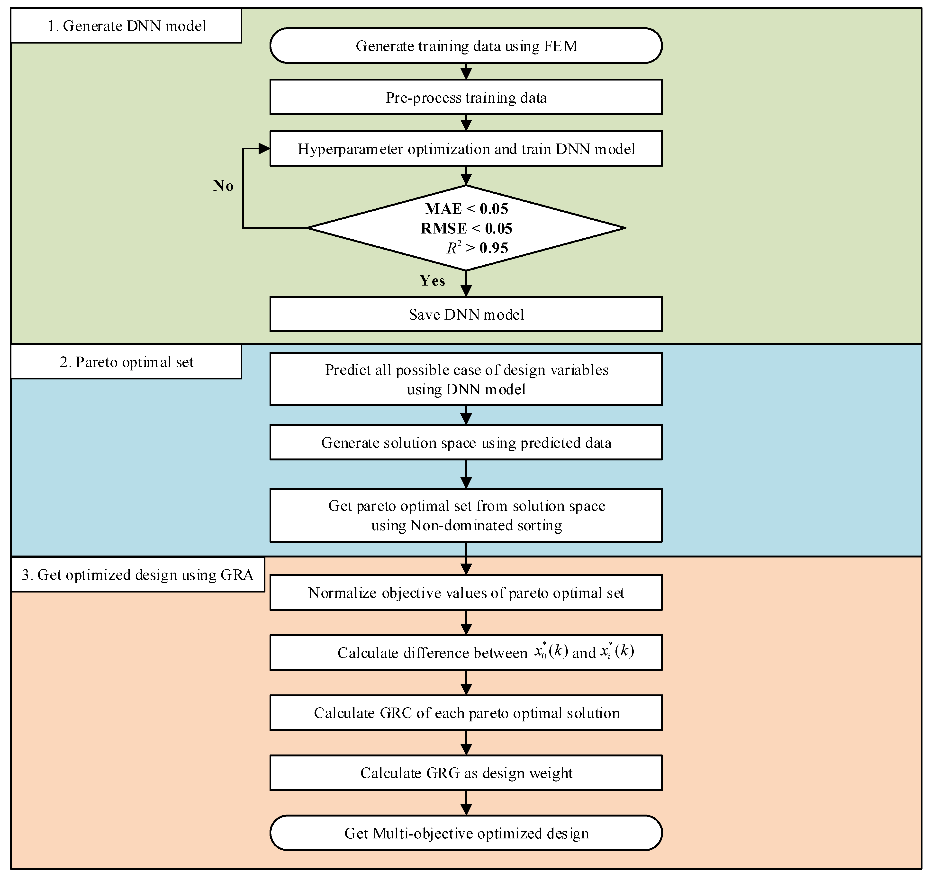
Figure 2.
Schematic architecture of the deep neural network.
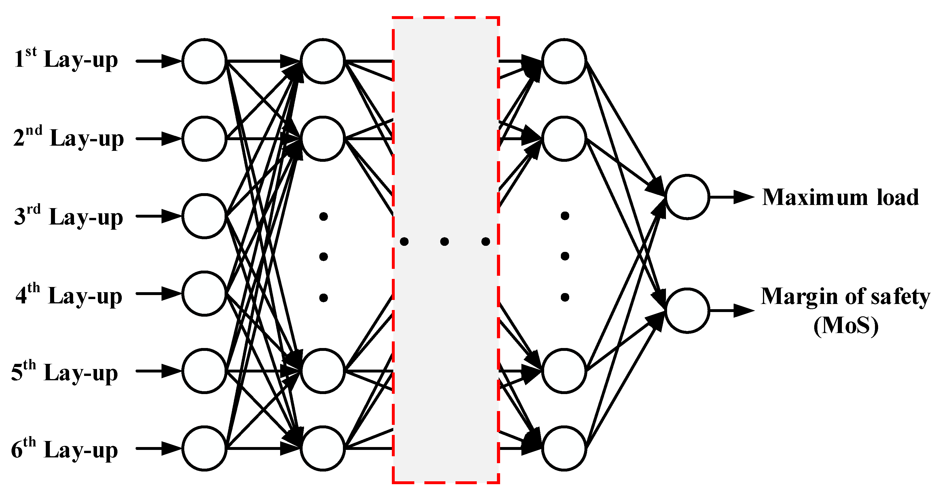
Figure 3.
Schematic diagram of feasible region and non-dominated point: (a) Representation of decision space and feasible region; (b) Concept of dominance and non-dominance.
Figure 3.
Schematic diagram of feasible region and non-dominated point: (a) Representation of decision space and feasible region; (b) Concept of dominance and non-dominance.
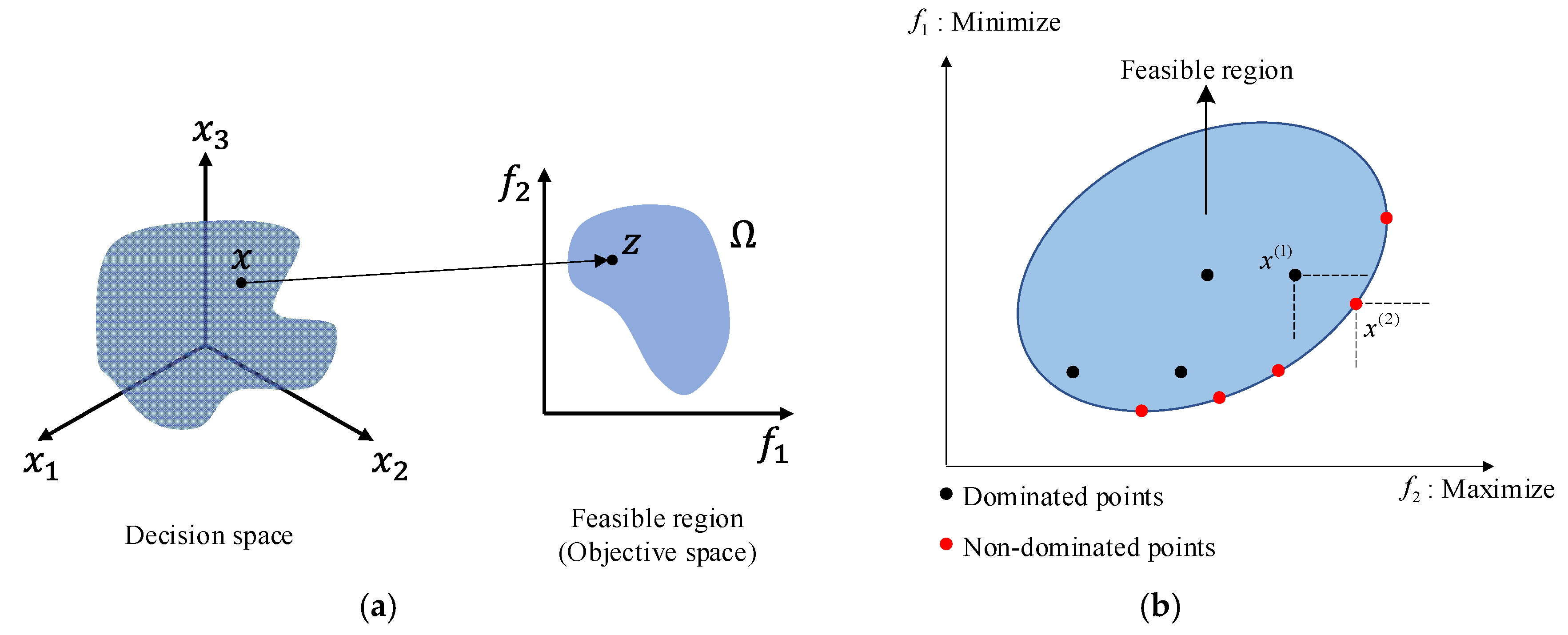
Figure 4.
Flowchart of non-dominated point sorting.
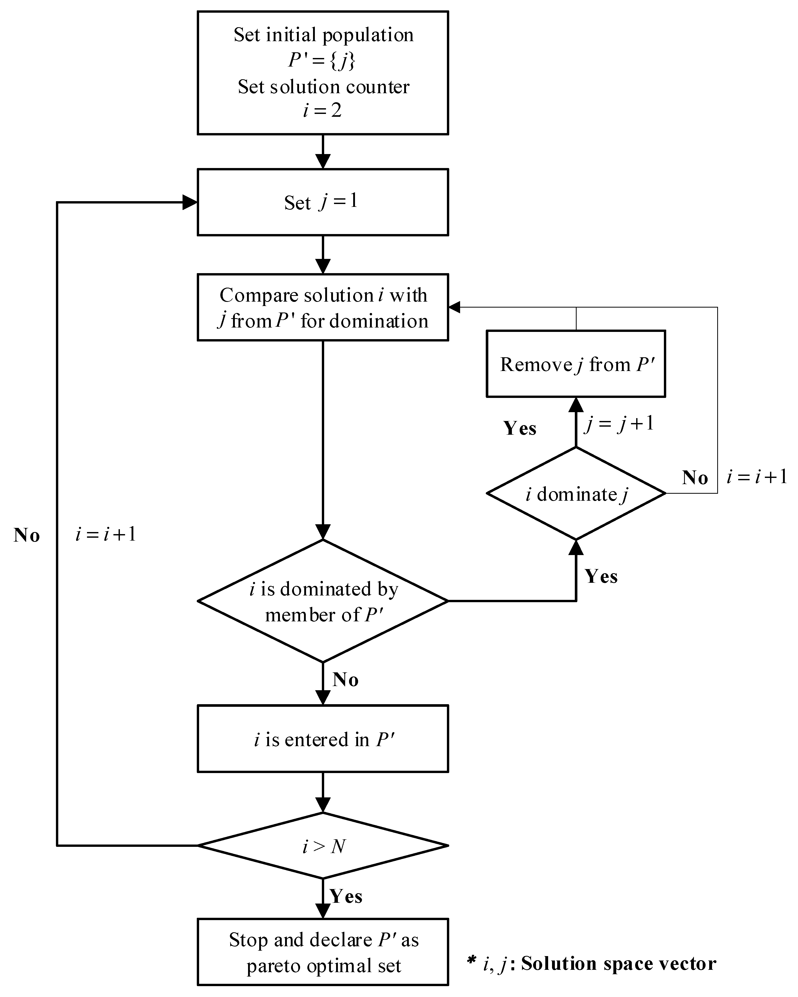
Figure 5.
3D model of Lab-scaled CFRP B-pillar.
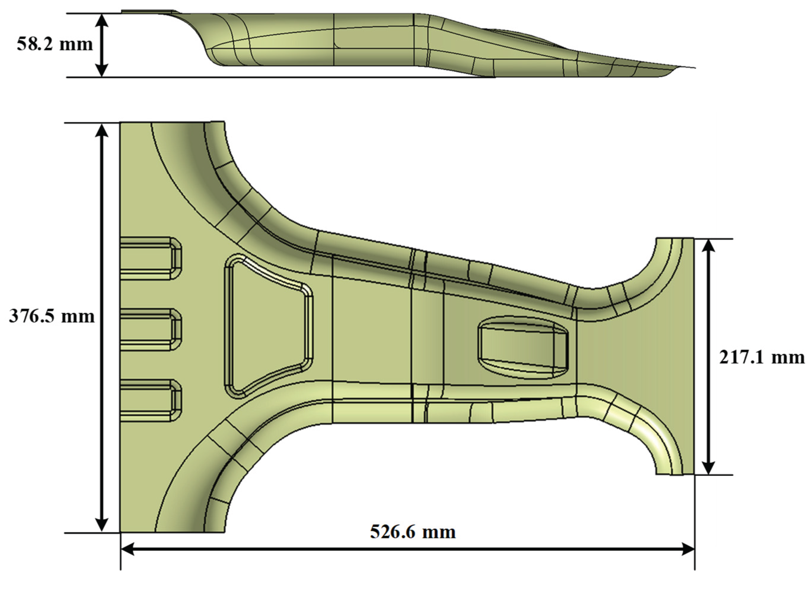
Figure 6.
Boundary condition and impact position of lab-size CFRP B-pillar simulation.
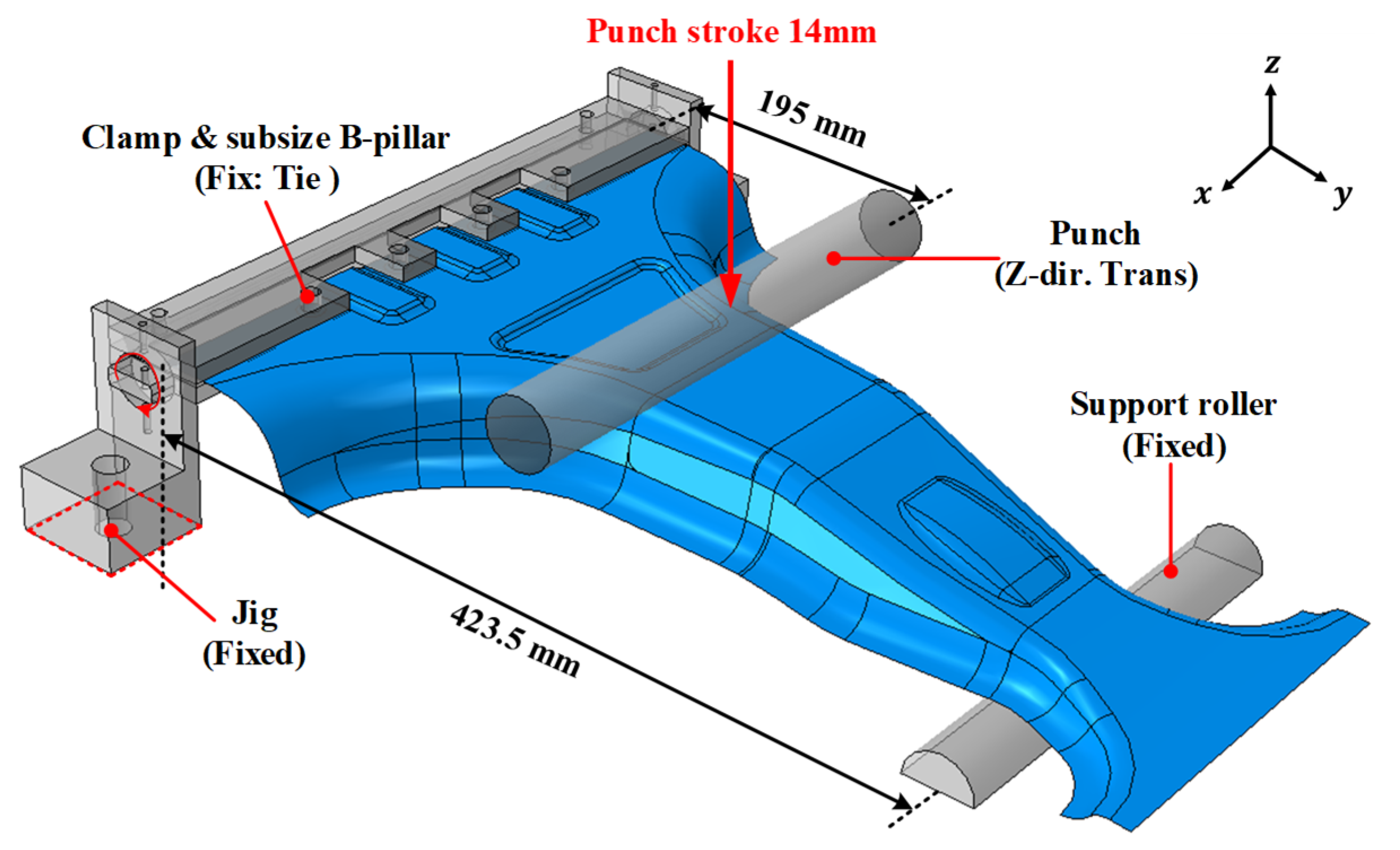
Figure 7.
Results of FE simulation for 0°lay-up configuration of the lab-scaled CFRP B-pillar. (a) Failure index; (b) Stroke-force curve.
Figure 7.
Results of FE simulation for 0°lay-up configuration of the lab-scaled CFRP B-pillar. (a) Failure index; (b) Stroke-force curve.
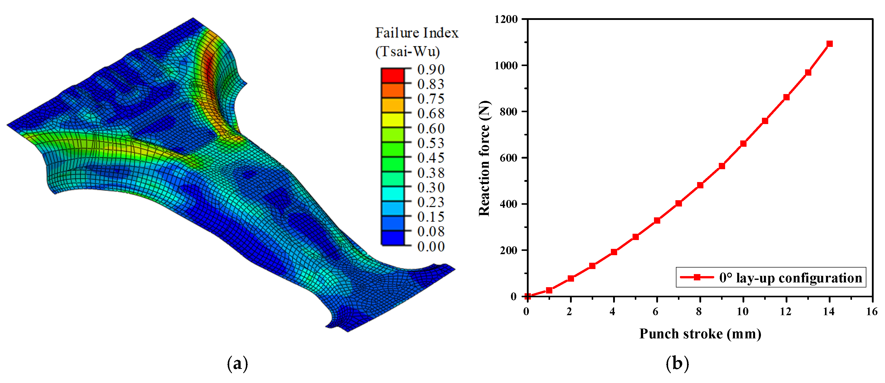
Figure 8.
Solution space and pareto optimal set.
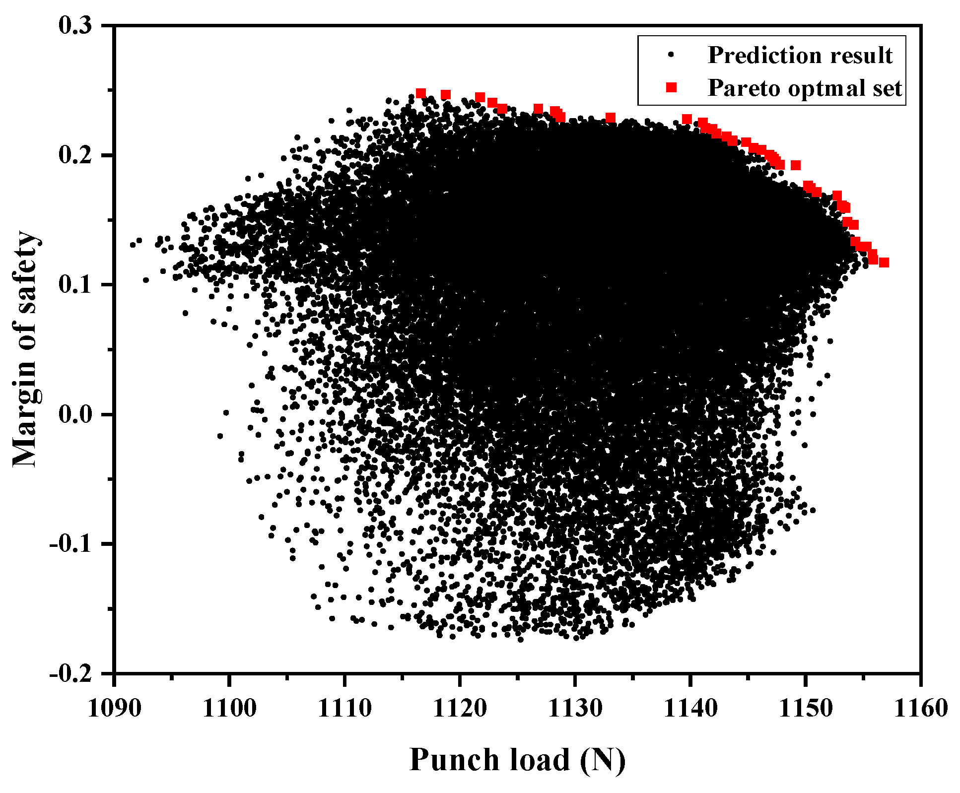
Figure 9.
Performance comparison about each lay-up.
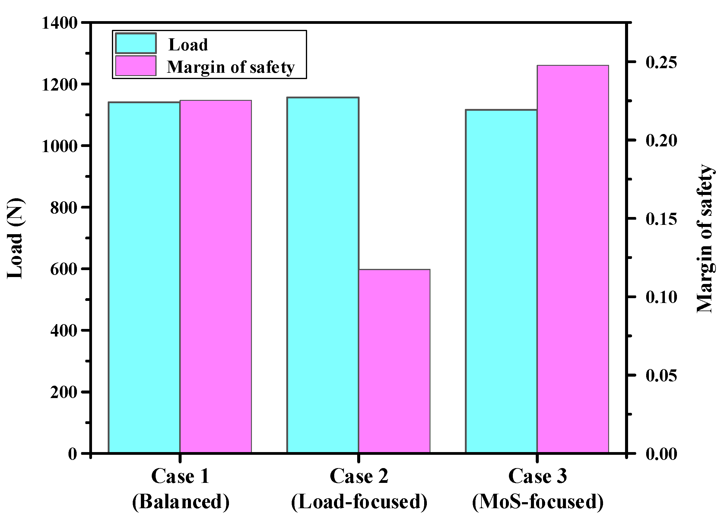
Figure 10.
Experimental equipment for manufacturing of lab-size CFRP B-Pillar.
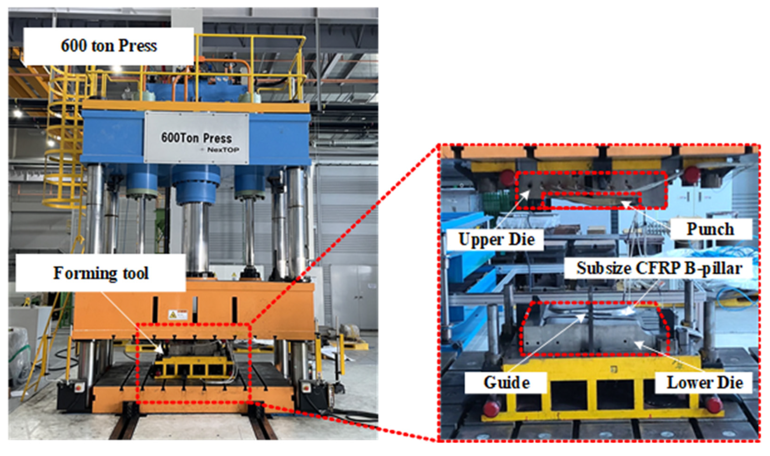
Figure 11.
Experimental results of manufacturing lab-scale CFRP B-pillar through PCM process. (a) Before forming; (b) After forming.
Figure 11.
Experimental results of manufacturing lab-scale CFRP B-pillar through PCM process. (a) Before forming; (b) After forming.
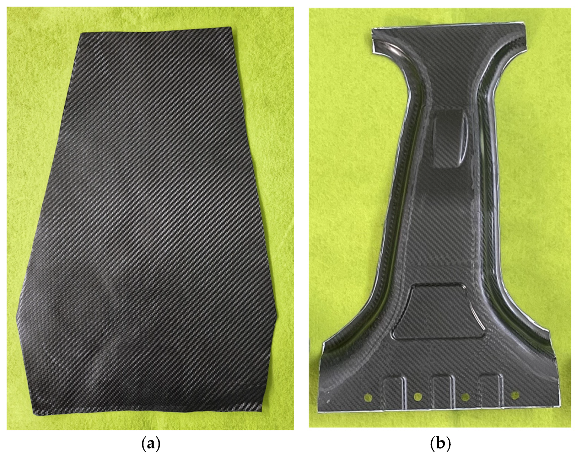
Figure 12.
Experimental apparatus for bending experiment of Lab-size CFRP B-Pillar.
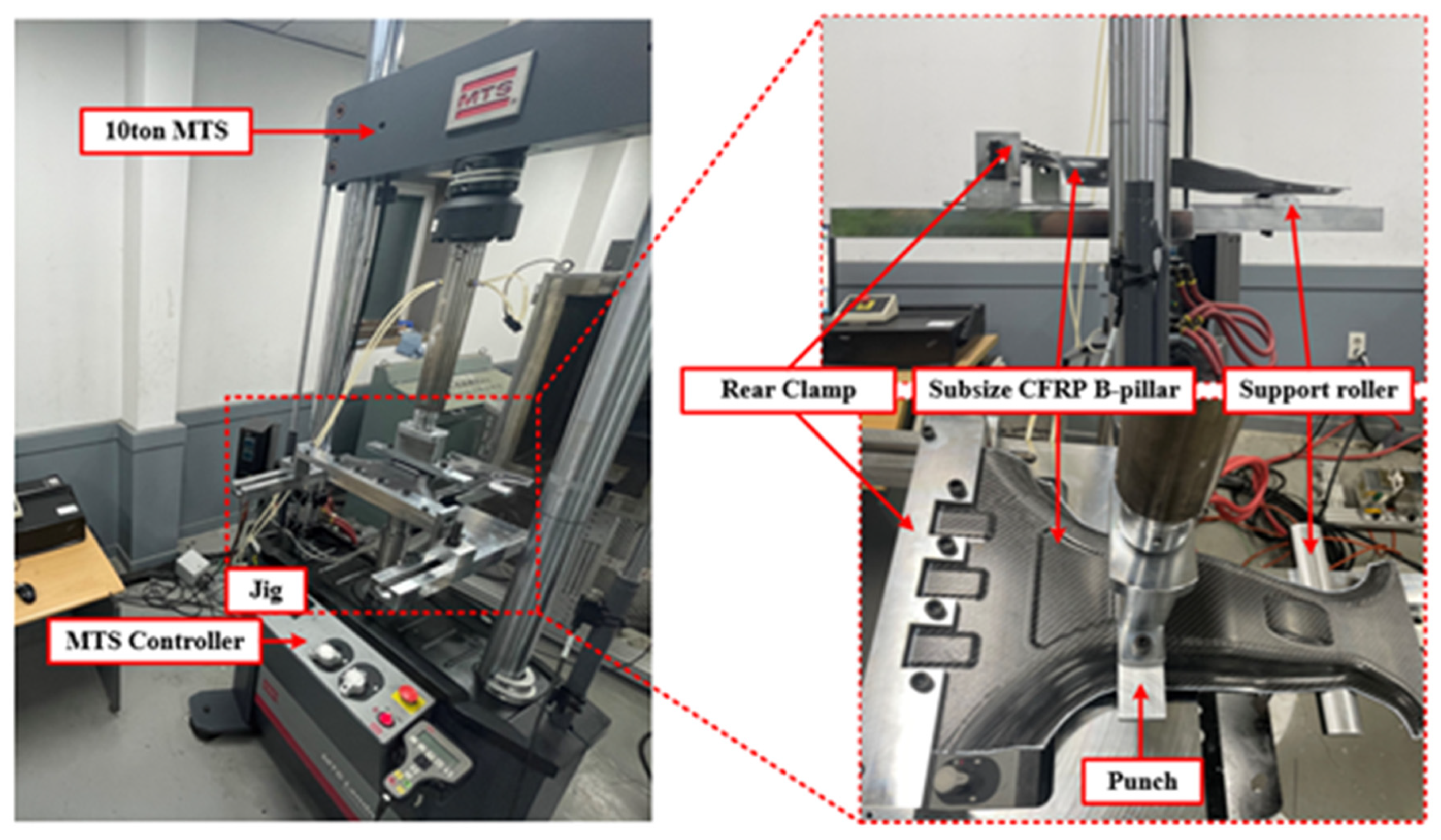
Figure 13.
Results of bending experiment for each lay-up cases.
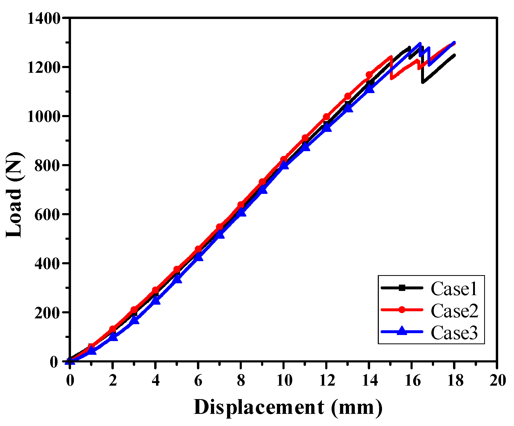
Figure 14.
FEM results of initial crack locations for each lay-up case. (a) Case 1: Balanced; (b) Case 2: Load-focused; (c) Case 3: MoS-focused.
Figure 14.
FEM results of initial crack locations for each lay-up case. (a) Case 1: Balanced; (b) Case 2: Load-focused; (c) Case 3: MoS-focused.
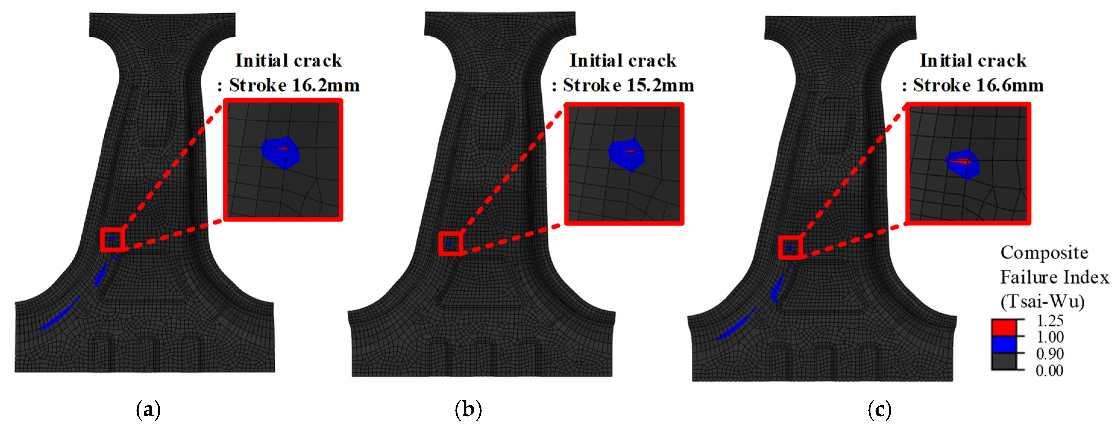
Figure 15.
Comparison of Experiment and FEM result at punch stroke 18mm. (a) case 1; (b) Case 2; (c) Case 3.
Figure 15.
Comparison of Experiment and FEM result at punch stroke 18mm. (a) case 1; (b) Case 2; (c) Case 3.
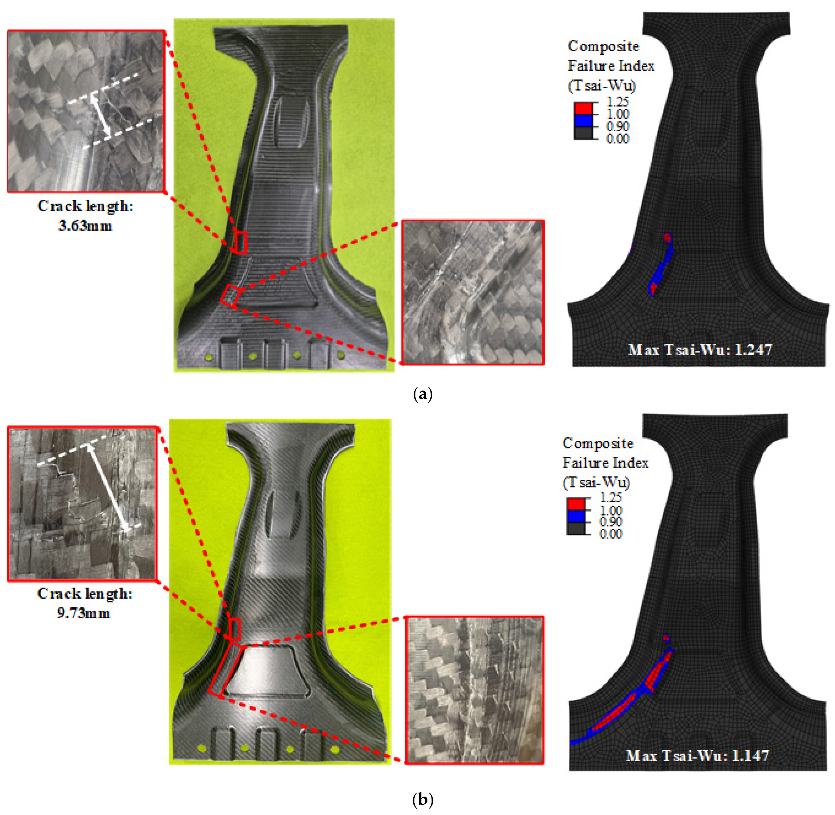
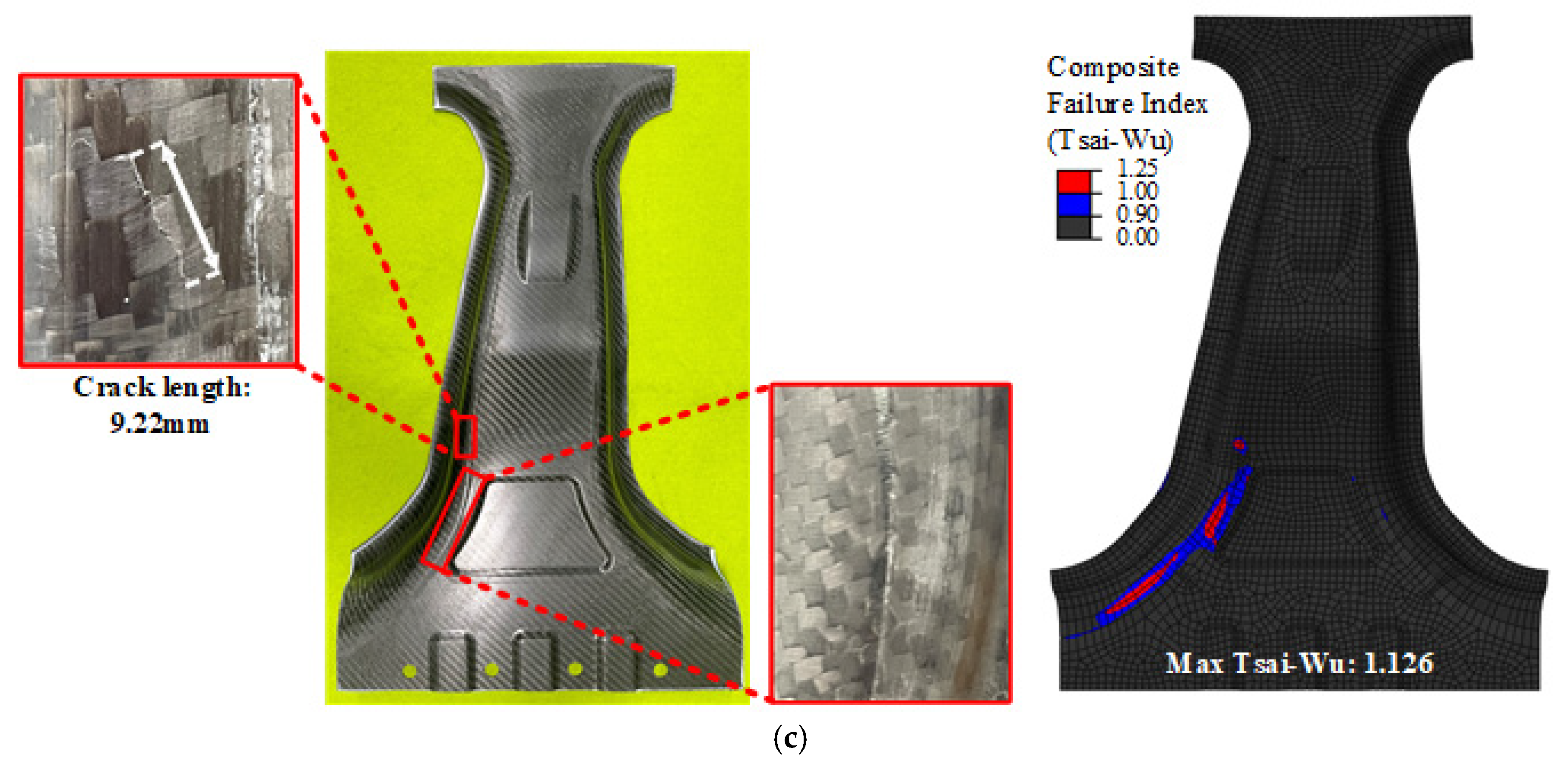

Table 1.
Mechanical properties of CFRP laminate for structure analysis [27].
Table 1.
Mechanical properties of CFRP laminate for structure analysis [27].
| Property | Symbol | Value |
| Elastic Modulus in fiber direction (GPa) | 65.01 | |
| Elastic Modulus in transverse direction (GPa) | 65.01 | |
| Poisson’s ratio in 1-2 | 0.13 | |
| Shear Modulus in 1-2 (GPa) | 12.69 | |
| Shear Modulus in 2-3 (GPa) | 1.38 | |
| Shear Modulus in 1-3 (GPa) | 1.38 | |
| Mass Density (g/cm2) | 1.52 |
Table 2.
Strength of CFRP.
| Property | Symbol | Value |
| Tensile stress in fiber direction (MPa) | 638 | |
| Compressive stress in fiber direction (MPa) | 494 | |
| Tensile stress in transverse direction (MPa) | 633 | |
| Compressive stress in transverse direction (MPa) | 491 | |
| Shear strengh (MPa) | 106 |
Table 3.
Load and MoS according to punch stroke.
| Layup | Punchstroke:12mm | Punchstroke:14mm | Punchstroke:16mm | ||||||||
| Load(N) | MoS | Load(N) | MoS | Load(N) | MoS | ||||||
| 0 | 60 | 30 | 0 | 60 | 0 | 1001.79 | 0.3024 | 1127.38 | -0.8993 | 1406.14 | -0.0909 |
| 0 | 30 | 30 | 40 | 75 | 0 | 990.23 | 0.2795 | 1114.38 | 0.0580 | 1388.32 | -0.1039 |
| 15 | 0 | 75 | 45 | 0 | 45 | 1002.99 | 0.2230 | 1128.53 | 0.0092 | 1409.18 | -0.1460 |
| 30 | 75 | 75 | 45 | 75 | 75 | 993.98 | 0.4222 | 1118.33 | 0.1563 | 1394.56 | -0.0982 |
| 30 | 0 | 45 | 15 | 0 | 15 | 999.21 | 0.2794 | 1124.75 | 0.0704 | 1403.85 | -0.0917 |
| 45 | 75 | 15 | 15 | 30 | 60 | 1021.02 | 0.3310 | 1146.93 | 0.0897 | 1432.99 | -0.0982 |
| 45 | 45 | 30 | 30 | 45 | 60 | 1006.32 | 0.3192 | 1129.89 | 0.0908 | 1411.61 | -0.0974 |
| 60 | 75 | 60 | 0 | 45 | 0 | 999.99 | 0.1462 | 1125.06 | -0.0328 | 1405.09 | -0.1714 |
| 75 | 60 | 15 | 60 | 45 | 15 | 1004.29 | 0.2235 | 1130.30 | 0.0291 | 1412.38 | -0.1204 |
| 75 | 60 | 0 | 75 | 30 | 15 | 993.39 | 0.1967 | 1118.33 | 0.0071 | 1396.99 | -0.1394 |
Table 4.
Structure and parameter of DNN model.
| Parameter | Value |
| Initial dataset | 100% (2,000) |
| Training dataset | 70% (1,400) |
| Test dataset | 15% (300) |
| Validation dataset | 15% (300) |
| Training data sampling method | Random sampling |
| Data normalization method | Min-Max normalization |
| Maximum iteration | 300 |
| Learning rate | 0.001 |
| Activation function | ReLU |
| Optimization algorithms | Adam |
| Hidden layer / Node | 5 / 1,000 |
Table 5.
Prediction performance of trained DNN model.
| TestdatasetError | ||
| MAE | RMSE | R2 |
| 0.023 | 0.038 | 0.978 |
Table 6.
Pareto optimal set and results of GRG.
| No | Layup | GRCLoad | GRCMoS | GRG1 | GRG2 | GRG3 | |||||
| 1 | 0 | 45 | 45 | 15 | 0 | 45 | 0.7338 | 0.8079 | 0.7709 | 0.7412 | 0.8005 |
| 2 | 0 | 45 | 45 | 30 | 0 | 45 | 0.7214 | 0.8297 | 0.7756 | 0.7323 | 0.8189 |
| 3 | 0 | 45 | 45 | 30 | 60 | 60 | 0.5888 | 0.8769 | 0.7329 | 0.6176 | 0.8481 |
| 4 | 0 | 45 | 45 | 45 | 60 | 60 | 0.5418 | 0.9482 | 0.7450 | 0.5824 | 0.9075 |
| 5 | 0 | 45 | 45 | 60 | 60 | 60 | 0.5139 | 0.9941 | 0.7540 | 0.5620 | 0.9461 |
| 6 | 0 | 45 | 60 | 0 | 15 | 45 | 0.7500 | 0.7837 | 0.7683 | 0.7560 | 0.7806 |
| 7 | 0 | 45 | 60 | 15 | 0 | 45 | 0.7296 | 0.8263 | 0.7780 | 0.7394 | 0.8167 |
| 8 | 0 | 45 | 60 | 15 | 15 | 45 | 0.7463 | 0.7978 | 0.7721 | 0.7515 | 0.7926 |
| 9 | 0 | 45 | 60 | 30 | 0 | 45 | 0.7187 | 0.8532 | 0.7860 | 0.7322 | 0.8397 |
| 10 | 0 | 45 | 60 | 30 | 60 | 60 | 0.5866 | 0.8946 | 0.7407 | 0.6175 | 0.8638 |
| 11 | 0 | 45 | 60 | 45 | 0 | 45 | 0.7014 | 0.8689 | 0.7852 | 0.7182 | 0.8521 |
| 12 | 0 | 45 | 60 | 45 | 0 | 60 | 0.6287 | 0.8756 | 0.7521 | 0.6534 | 0.8509 |
| 13 | 0 | 45 | 60 | 45 | 60 | 45 | 0.5847 | 0.9049 | 0.7448 | 0.6168 | 0.8729 |
| 14 | 0 | 45 | 60 | 45 | 60 | 60 | 0.5341 | 0.9774 | 0.7558 | 0.5785 | 0.9331 |
| 15 | 0 | 45 | 60 | 45 | 75 | 60 | 0.5481 | 0.9175 | 0.7328 | 0.5851 | 0.8806 |
| 16 | 0 | 45 | 60 | 60 | 60 | 45 | 0.5727 | 0.9171 | 0.7449 | 0.6072 | 0.8827 |
| 17 | 0 | 45 | 60 | 60 | 60 | 60 | 0.5000 | 1.0000 | 0.7500 | 0.5500 | 0.9500 |
| 18 | 15 | 45 | 60 | 0 | 15 | 45 | 0.8398 | 0.7016 | 0.7708 | 0.8261 | 0.7154 |
| 19 | 15 | 45 | 60 | 0 | 30 | 45 | 0.8106 | 0.7128 | 0.7617 | 0.8008 | 0.7226 |
| 20 | 15 | 45 | 60 | 0 | 45 | 30 | 0.8161 | 0.7031 | 0.7596 | 0.8048 | 0.7144 |
| 21 | 15 | 45 | 60 | 15 | 15 | 45 | 0.8014 | 0.7339 | 0.7677 | 0.7947 | 0.7407 |
| 22 | 15 | 45 | 75 | 15 | 15 | 45 | 0.8081 | 0.7216 | 0.7649 | 0.7995 | 0.7302 |
| 23 | 15 | 60 | 45 | 0 | 15 | 45 | 0.8090 | 0.7132 | 0.7612 | 0.7995 | 0.7228 |
| 24 | 15 | 60 | 45 | 0 | 60 | 30 | 0.7906 | 0.7499 | 0.7703 | 0.7866 | 0.7539 |
| 25 | 15 | 60 | 60 | 0 | 15 | 45 | 0.8053 | 0.7269 | 0.7661 | 0.7975 | 0.7348 |
| 26 | 15 | 60 | 60 | 0 | 60 | 30 | 0.7800 | 0.7564 | 0.7682 | 0.7777 | 0.7587 |
| 27 | 15 | 60 | 60 | 15 | 60 | 30 | 0.7703 | 0.7762 | 0.7733 | 0.7709 | 0.7756 |
| 28 | 15 | 60 | 60 | 30 | 75 | 30 | 0.7536 | 0.7810 | 0.7673 | 0.7564 | 0.7783 |
| 29 | 30 | 60 | 0 | 45 | 15 | 45 | 0.8634 | 0.6408 | 0.7521 | 0.8412 | 0.6631 |
| 30 | 30 | 60 | 0 | 60 | 15 | 45 | 0.8592 | 0.6471 | 0.7532 | 0.8380 | 0.6684 |
| 31 | 30 | 60 | 15 | 0 | 15 | 45 | 0.9262 | 0.5678 | 0.7470 | 0.8904 | 0.6037 |
| 32 | 30 | 60 | 15 | 0 | 30 | 45 | 0.9383 | 0.5626 | 0.7505 | 0.9008 | 0.6002 |
| 33 | 30 | 60 | 60 | 0 | 15 | 45 | 0.9208 | 0.5980 | 0.7594 | 0.8885 | 0.6303 |
| 34 | 30 | 60 | 60 | 0 | 30 | 45 | 0.9165 | 0.6010 | 0.7588 | 0.8850 | 0.6325 |
| 35 | 30 | 60 | 60 | 0 | 60 | 30 | 0.9232 | 0.5960 | 0.7597 | 0.8906 | 0.6288 |
| 36 | 30 | 60 | 75 | 0 | 60 | 30 | 0.9081 | 0.6232 | 0.7657 | 0.8797 | 0.6517 |
| 37 | 30 | 60 | 75 | 30 | 60 | 30 | 0.8725 | 0.6315 | 0.7520 | 0.8484 | 0.6556 |
| 38 | 45 | 30 | 0 | 0 | 30 | 45 | 0.9755 | 0.5128 | 0.7442 | 0.9293 | 0.5591 |
| 39 | 45 | 30 | 0 | 0 | 45 | 45 | 0.9641 | 0.5249 | 0.7445 | 0.9202 | 0.5688 |
| 40 | 45 | 30 | 0 | 15 | 60 | 30 | 0.9512 | 0.5253 | 0.7383 | 0.9086 | 0.5679 |
| 41 | 45 | 45 | 0 | 0 | 15 | 45 | 0.9772 | 0.5043 | 0.7408 | 0.9300 | 0.5516 |
| 42 | 45 | 45 | 0 | 0 | 30 | 45 | 1.0000 | 0.5000 | 0.7500 | 0.9500 | 0.5500 |
| 43 | 45 | 60 | 0 | 0 | 15 | 45 | 0.9417 | 0.5334 | 0.7376 | 0.9009 | 0.5742 |
Table 7.
Error comparison between FE-simulation and predicted value through DNN model.
| GRG1(Balanced) | GRG2 (Load-focused) | GRG3 (MoS-focused) | ||||
| Load(N) | MoS | Load(N) | MoS | Load(N) | MoS | |
| FEM | 1143.86 | 0.2159 | 1157.47 | 0.1179 | 1117.25 | 0.2401 |
| DNN | 1141.05 | 0.2253 | 1156.78 | 0.1173 | 1116.59 | 0.2477 |
| Error (%) | 0.25 | 4.35 | 0.06 | 0.51 | 0.06 | 3.17 |
Table 8.
Error comparison between FE-simulation and experiment at punch stroke 14mm.
| Case 1(Balanced) | Case 2 (Load-focused) | Case 3 (MoS-focused) | ||||
| Load(N) | Initial fracture stroke (mm) | Load(N) | Initial fracture stroke (mm) | Load(N) | Initial fracture stroke (mm) | |
| FEM | 1143.86 | 16.20 | 1157.47 | 15.20 | 1117.25 | 16.60 |
| Experiment | 1131.46 | 15.91 | 1164.83 | 15.05 | 1106.33 | 16.40 |
| Error (%) | 1.08 | 1.79 | 0.64 | 0.99 | 0.98 | 1.20 |
Disclaimer/Publisher’s Note: The statements, opinions and data contained in all publications are solely those of the individual author(s) and contributor(s) and not of MDPI and/or the editor(s). MDPI and/or the editor(s) disclaim responsibility for any injury to people or property resulting from any ideas, methods, instructions or products referred to in the content. |
© 2025 by the authors. Licensee MDPI, Basel, Switzerland. This article is an open access article distributed under the terms and conditions of the Creative Commons Attribution (CC BY) license (http://creativecommons.org/licenses/by/4.0/).
Copyright: This open access article is published under a Creative Commons CC BY 4.0 license, which permit the free download, distribution, and reuse, provided that the author and preprint are cited in any reuse.


