
Submitted:
29 September 2025
Posted:
30 September 2025
You are already at the latest version
Abstract
Bahir Dar City, Ethiopia, is experiencing rapid urbanization and motorization, leading to major transportation challenges characterized by uneven travel demand and variable trip durations. This study investigates how departure times influence trip duration and mode choice by integrating activity-based models (ABMs) with machine learning techniques. The combined approach enhances predictive accuracy and offers deeper insights into the temporal dynamics of travel behavior. Using population synthesis with PopulationSim and activity execution modelling in VISUM, a total of 147,351 activities, 56,121 tours, and 112,429 trips were generated. Results reveal strong temporal variations in mobility, with peak demand observed around 8 AM, 12 PM, 1 PM, 2 PM, and 5 PM. Minibuses dominate urban mobility during these periods, while auto-rickshaws provide flexible options for medium-distance travel. Analysis of trip durations shows that buses and minibuses experience the greatest variability due to congestion and operational delays, whereas private cars, walking, and auto-rickshaws demonstrate greater stability. Machine learning results indicate that Random Forest (R² = 0.769, RMSE = 3.78) outperforms XGBoost and MLP in predicting trip durations and capturing peak-hour dynamics. These findings underscore the critical role of departure time in shaping travel outcomes and suggest the need for coordinated land use and transport policies to balance demand, improve reliability, and support sustainable mobility.
Keywords:
Travel behavior
; Departure time
; Activity-based model
; Trip duration
; Mode choice
; Machine learning
; Random Forest
; Travel time reliability
; Land use
1. Introduction
1.1. Background
Travel demand models are important in measuring the influence of policies, infrastructure investments, and demographic shifts on travel behavior and traffic volumes [1]. Transportation models were crucial to predict transport demand and assess the impacts of various policies since the late 1950s. The initial generation of models during this time and the early 1960s was purposely designed to predict future transport demand to help inform road capacity planning. These models, commonly known as four-step models, operate at the traffic zone level and aggregate individuals based on their respective zones.
Four-Step Models (FSMs) analyze travel demand at an aggregate level through a structured framework comprising four stages [2]: trip distribution, which identifies the destinations of these trips; mode split, which determines the chosen mode of transport (such as car, bus, or walking); and traffic assignment, which allocates trips to specific routes. However, there are visible problems in the four-step models, such as a lack of behavioral content can complicate the evaluation of policies like traffic demand management.
Their aggregation and supply-focused nature also hinders the prediction of individual behavioral responses. As a result, a transition towards disaggregate modelling occurred in the 1970s and 1980s, emphasizing individual and household decision-making processes [3].
Activity-based models (ABMs) are designed to estimate individual travel patterns, thereby enhancing the accuracy of forecasts for aggregated travel demand [4].
For developing an effective transportation system, urban planning, and public policy, it is important to understand the direction of movements of individuals and communities through their environment. Travel patterns and preferences are basic characteristics of human behavior and urban systems. Activity-Based Models (ABM) are very crucial to analyze travel behaviors, and they can provide a more refined and diverse view of travel choices than traditional aggregation models.
Unlike conventional models that often summarize travel demand based on trips and origins destinations, ABM focuses on the underlying activities that generate travel, offering insights into the motivations and constraints shaping individual travel decisions.
In activity-based models, travel demand is derived from the individual’s need to engage in activities that are located across different spaces and times, in contrast to traditional analytical trip-based models [5]. This approach considers how various factors, including socio-demographics, land use, and external influences, affect travel behavior over time.
Despite advancements in transportation modelling, there remains a gap in accurately capturing the complexities of individual travel behaviors and preferences. Traditional models often rely on aggregate data, which may overlook the nuances of how different demographic groups interact with their transport environment.
While congestion levels, service frequency, and individual scheduling constraints vary across the day, departure time is a very important factor that can influence trip duration and mode choice. As discussed above, the traditional ABMs are good at capturing individual plans, linking, and adjusting their activities, and they can provide better insights than aggregate trip-based models. However, they have a weakness in high computational demands, complexity in calibration, and have limited ability in capturing nonlinear interactions between departure time, travel duration, and mode choice.
In contrast to ABMs, machine learning models are effective in capturing nonlinear relationships and handling large-scale data, which can then bring higher predictive accuracy. Despite these advantages, ML models are often criticized for being “black boxes,” lacking explicit behavioral interpretation and theoretical grounding in travel behavior.
Integrating ABM and ML offers a balanced approach. This is because ABM are good in interpretability, and ML can boost prediction accuracy and are effective in managing complex urban travel data. So, we can get deeper insights about the influence of departure time on travel time variability and mode choice. This is then very important to design strategies of congestion mitigation and sustainable mobility policies.
The objective of this study is to create a better understanding of current travel patterns and preferences using ABMs and ML techniques for Bahir Dar city.
1.2. Key Insights from Activity-Based Models (ABM) for Understanding Current Travel Patterns and Preferences
Activity-Based Models (ABM) offer essential insights into travel patterns and preferences by emphasizing the activities that drive travel rather than focusing solely on the travel itself. A notable insight from ABM is the recognition of the intricate interrelationships between different activities and the resulting travel behaviors. It highlights that travel is often a means to achieve specific goals, with individuals organizing their trips around a sequence of activities such as work, shopping, and leisure that need to be completed within a certain timeframe. This approach enables a deeper understanding of how factors like time constraints, trip purpose, and location influence individual travel choices [6].
ABM also highlights the importance of demographic factors, such as income, age, and household structure, in influencing travel behavior. The models demonstrate that various demographic groups exhibit distinct travel patterns, underscoring the need for tailored transportation solutions that cater to their specific needs.
Another critical insight from ABM is the influence of land use on travel behavior. Research indicates that mixed-use developments can significantly lower travel demand by allowing residents’ easier access to services and activities within walking distance, thereby promoting sustainable modes of transport like walking and cycling [7]. Additionally, modelling the duration and sequencing of activities provides valuable data for transportation planners and policymakers. By understanding how much time individuals dedicate to different activities, planners can better tailor transportation services and infrastructure to meet actual demand, leading to more efficient solutions.
Finally, ABM supports scenario analysis, enabling stakeholders to assess the potential effects of various policies or infrastructure changes on travel behavior. This predictive capability aids decision-making by offering a clearer understanding of how different strategies might impact travel patterns, ultimately enhancing the effectiveness of urban and transportation planning initiatives [8,9].
1.3. Statement of the Research Problem and Objectives
Bahir Dar city is experiencing challenges in transportation and urban planning, since there is a rapid growth in urbanization and motorization. Many of the residents transfer to the city Centre for work and other essential activities, and this causes high traffic congestion during peak hours. In contrast, there are fewer trips from the city Centre to Abay Mado and travel patterns are uneven. These unbalanced trips and travel demand make systems inefficient and help to emphasize the importance of understanding the effects of departure times on trip durations and mode choices. Activity-Based Models (ABMs) provide a valuable framework for capturing these travel behaviors in a comprehensive manner.
The core research problem addressed in this study is the limited understanding of how departure times influence trip duration and mode choice. To bridge this gap, the study integrates Activity-Based Modelling (ABM) with Machine Learning (ML) techniques to analyze travel patterns more effectively and to capture the complex interactions between departure time, travel duration, and mode selection.
2. Literature Review
2.1. Activity-Based Models Progress and Its Modelling Approaches in analysing travel behaviour
Travel demand modelling originally focused on trip-based four-step models as the standard approach. Subsequently, newer models, such as tour-based and activity-based modelling, emerged to address many of the limitations of conventional methods. The tour-based approach analyses chains of trips that begin and end at the same location as the individual unit of analysis, while the activity-based travel demand model views travel as a derived demand aimed at fulfilling individual needs[10]. The activity-based methodology for analyzing travel has been in use for more than twenty years, with its origins extending back to the pioneering research of Hägerstrand (1970) and his colleagues [11]. The 1990s marked the beginning of significant progress and gained popularity in the development of activity-based models of travel demand, responding to the limitations of previous generations of models[12,13]. According to[12,14,15], there are three distinct modelling approaches in the context of activity-based travel anavlysis. First, constraints-based models emphasize the limitations that affect individual behavior, considering various factors that restrict choices. Second, utility-maximizing models are centred on the principles of rational choice, focusing on how preferences influence decision-making. Lastly, computational process models employ algorithms to simulate behavior, allowing for a more dynamic representation of travel patterns and interactions. These approaches can provide valuable insights into understanding travel demand and activity patterns. Many studies integrated econometric and rule-based modelling methods in the ABM framework for better computational efficiency and results accuracy [14].
2.2. Activity-Based Travel Demand Model Components and Terminology
According to [8], ABM comprises four essential components that enable subsequent choices for each individual to meet the model’s objectives. The first component involves making several long-term decisions for each person (e.g., concerning ownership of a car, the location of school or work, etc.). Based on these decisions, the second component identifies the main daily activity purpose for each individual (e.g., work, leisure). Once this purpose is established, the third component generates and schedules the tours each person undertakes that day (e.g., home-work-home) and selects the preferred travel mode (e.g., car, train). The final component determines the individual trips that constitute each tour, scheduling these trips throughout the day and specifying the travel mode for each trip. While all components make decisions for each person at different levels of detail, they generally utilize the same discrete choice model, such as the multinomial logit model.
In addition to the components of the Activity-Based Travel Demand Model, [16] discusses the core features of ABMs despite the variations in technical details among existing systems. The first feature is the tour-based structure, where a tour defined as a closed chain of trips starting and ending at a base location serves as the main unit of analysis, ensuring consistency across trips by considering dimensions like destination, mode, and time of day. The second feature is the activity-based platform, which models travel as derived from daily activities, maintaining coherence in the typological, spatial, and temporal dimensions of individual activity patterns. The third feature is the micro-simulation modeling technique, which operates at a fully disaggregated level, converting probabilistic outcomes into definitive decisions among discrete choices.
According to [3], key terminology in activity-based modeling is presented as follows. An activity is the main business conducted at a location, including any waiting time (e.g., shopping at a shop). Activities can be categorized based on their purpose, have their own timing, i.e., the time when the activity occurs, and frequency, i.e., how often the activity is done within the specified time. A destination is a specific location where an activity is taking place, and this can be characterized by travel time and facility quality. The other key term is trip, which indicates the movement of destinations made through a transport mode. The other is a program for an activity, a list of activities to be performed in a day and the details of how these activities are organized in time and space. An activity pattern is the actual activities performed and their sequence. The physical environment and institutional environment represent the spatial layout and transport connections between locations and rules that control time usage which affects opportunities and limitations for participation in activities, respectively.
2.3. Machine Learning Applications in Transportation Modelling
ML is becoming a solution for everyday tasks, which include data analysis up to classification to text recommendation, and perception [17]. This broad application of ML shows that it can also address challenges of urban mobility. There are four types of machine learning, i.e., supervised, unsupervised, semi-supervised, and reinforcement learning, and to boost the performance of doing tasks, machine learning extracts patterns from data [18].
This study utilized supervised learning methods, specifically Random Forest, XGBoost, and Multilayer perceptron (MLP).
RF is an ensemble model which uses the combination of multiple decision trees to boost the accuracy of prediction. It is a model which is effective and widely used in pattern recognition tasks [19].
An XGBoost is also an ensemble learning model that uses decision trees as base learners, and it is well-designed for efficiency and scalability. This makes the model powerful for both regression and classification tasks.[20]
A Multilayer Perceptron (MLP) is a type of feed-forward neural network that has no cycles or loops. It includes an input layer, one or more hidden layers, and an output layer. Through supervised learning, MLPs transform input data into feature representations by using weighted connections between layers, which allows for effective classification and prediction[21].
Machine Learning algorithms provide a valuable opportunity for developing advanced activity–travel behavior models, particularly in cases where the underlying data distribution or functional relationships are unknown and when the primary objective is achieving high prediction accuracy rather than model interpretability[18]
2.4. Related Work, Novelty, and Research Gap
Several studies have utilized Activity-Based Models (ABMs) to analyze travel behavior in various urban contexts. Let us take a look at these studies one by one.
A study explicitly models the interactions between individuals participating in the same activities and temporal and physical constraints with an ABM framework [22]. They applied their model to the Naples metropolitan area, and they found a good balance between accuracy and operational feasibility. From these, we can understand that ABMs can provide more realistic origin/destination matrices and elasticity to network changes that can enhance transportation policy analysis. Building on this disaggregate approach, [23] presented a discrete choice activity schedule model system that can be specified and estimated from available data. The model can clearly represent tours and their interrelationships by capturing the interactions between an individual’s decisions throughout a 24-hour day. This helps to improve travel forecasts by capturing activity-based policy responses. Others also further explored the theoretical underpinning of ABMs than the practical applications. [11] Demonstrated the potential of network-based formulations from operations research to advance the general development of the ABM approach. Their mathematical programming formulation provides an analytical framework that unifies the complex interactions among the resource allocation decisions made by households, while preserving the utility-maximizing principles presumed to guide such decisions. Furthermore, they demonstrated that ABMs and traditional trip-based modeling methodologies are directly related, highlighting a connection between the two approaches. In a practical application of ABMs, [10] developed a single activity tour generation model and mode choice model. They identified the most important variables, i.e., age, income, license, distance, vehicle ownership, time of day, and cost of travel, using multimodal logit. These models can be used to predict activity patterns and mode preferences, serving as a platform for long-term transportation and land use planning.[18] Reviewed the activity-travel behaviour literature that employs Machine Learning (ML) techniques for empirical analysis and modelling. The study was focused on identifying trends in activity-travel behaviour research that apply machine learning, and they found that decision trees are a widely applied and the most versatile method, especially in the ALBATROSS MODEL. They also stated that, although no model is best at every condition, the ensemble models RF and XGBoost provided better prediction accuracy. Although machine learning offers promising opportunities for transportation analysis, its broader application is hindered by challenges such as limited collaboration between ML specialists and transportation planners, ambiguous problem definitions, and the scarcity of open-access datasets[24].
The novelty of this research lies in expanding the ABM framework by taking departure times as the basic factors affecting both trip duration and mode choice. Most previous studies on ABM focused on socio-demographic and spatial variables, but temporal variables, like departure time, travel duration, and mode choice, are not considered. This study also integrated ABM and machine learning models to capture the complex, non-linear relationships between departure time, travel duration, and mode choice.
This methodological advancement not only boosts predictive accuracy but also offers deeper insights into the temporal dynamics of travel behavior, thereby improving ABMs’ ability to reflect real-world travel decisions.
This study also contributes to a deep understanding of travel behavior, focusing on unique travel dynamics, especially the imbalanced distribution of foot traffic and transportation demand in Bahir Dar city throughout the day. Such understanding is critical for developing effective urban planning and transportation strategies that can accommodate the growing population while ensuring a balanced approach to urban development. By identifying how departure times shape travel behavior, transportation systems can be designed to reduce congestion, improve accessibility, and enhance the overall efficiency of urban mobility. So, this study provides valuable and context-specific insights into Bahir Dar city to fill the gaps in the literature.
3. Study Area and Methodology
3.1. Study Area
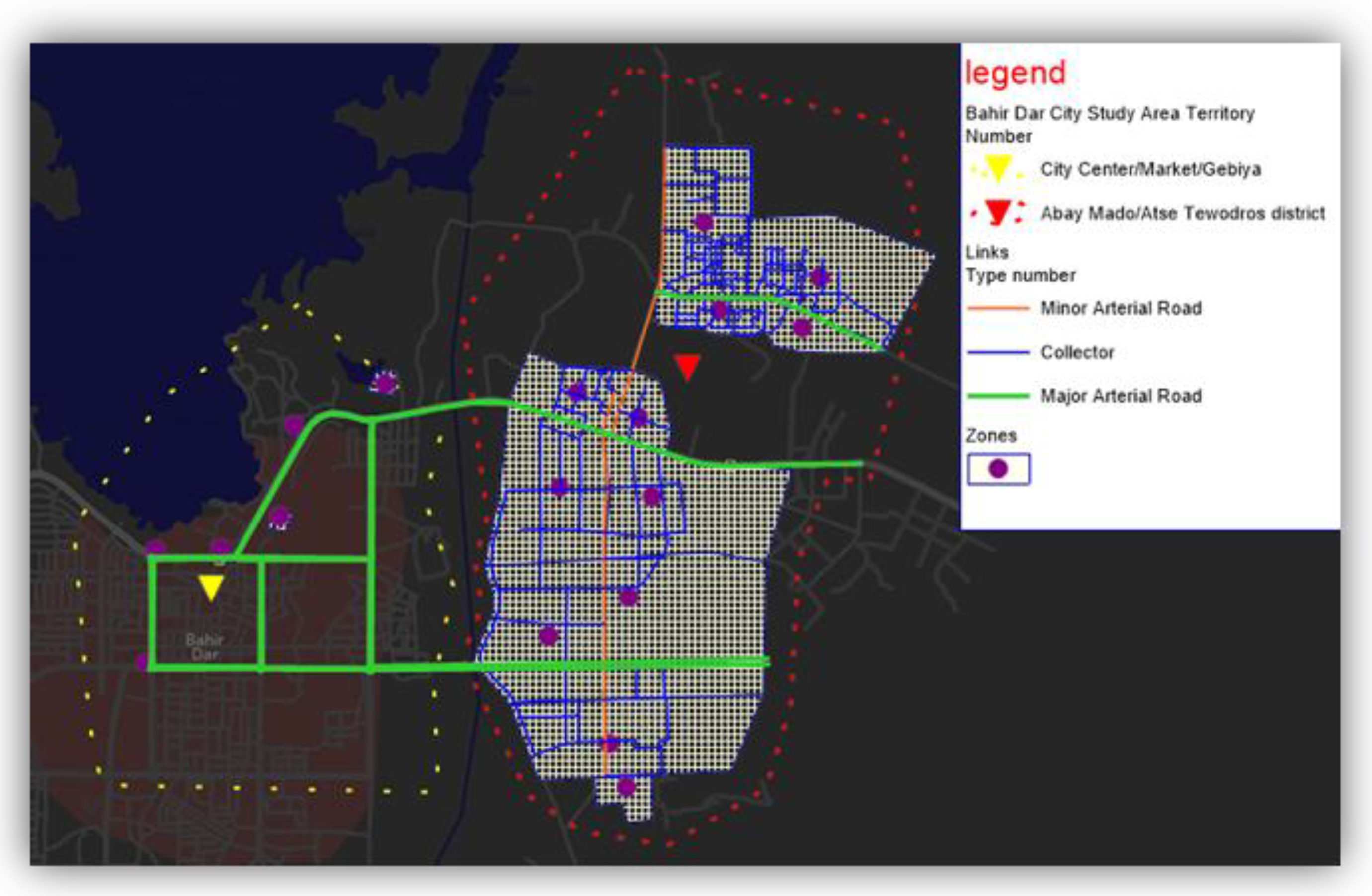
Bahir Dar has been undergoing rapid demographic expansion and accelerated spatial growth [25], is experiencing substantial challenges due to rapid urbanization and motorization. The concentration of public institutions, marketplaces, hospitals, leisure facilities, and spiritual sites, are concentrated in the central areas of Giorgis and Gebiya, and this creates an increased travel demand to the city centre. This has created a distinct imbalance in travel flows between the core and peripheral areas.
The Atse Tewodros District (commonly known as Abay Mado, outlined in the figure below with a red dotted boundary) consists of five kebeles and has a population of approximately 47,000 residents. It is one of the peripheral districts of the city. The Gabiya/City Center, outlined with a yellow dotted boundary in the figure, serves as the primary destination area for residents of Abay Mado. In the morning, most of the trips are from Abay Mado to the city centre, and there are a few trips from the city centre to Abay Mado. During Midday, the travel becomes balanced on both sides, since differences in demand remain evident. By evening, the flow is largely reversed, with significant return trips to Abay Mado and limited movement toward the city center.
This imbalance, which is visible in spatial and temporal distributions, shows that there is an urgent need to targeted interventions in urban planning and transportation management. Addressing these problems is key to ensuring efficiency, accessibility, and equity in the city’s transport system. Considering this problem, this study investigates travel behaviour in Bahir Dar using ABM and advanced machine learning models. It mainly focuses on the role of departure time in determining trip durations and mode choices.
Figure 1.
Study area (Bahir Dar City).
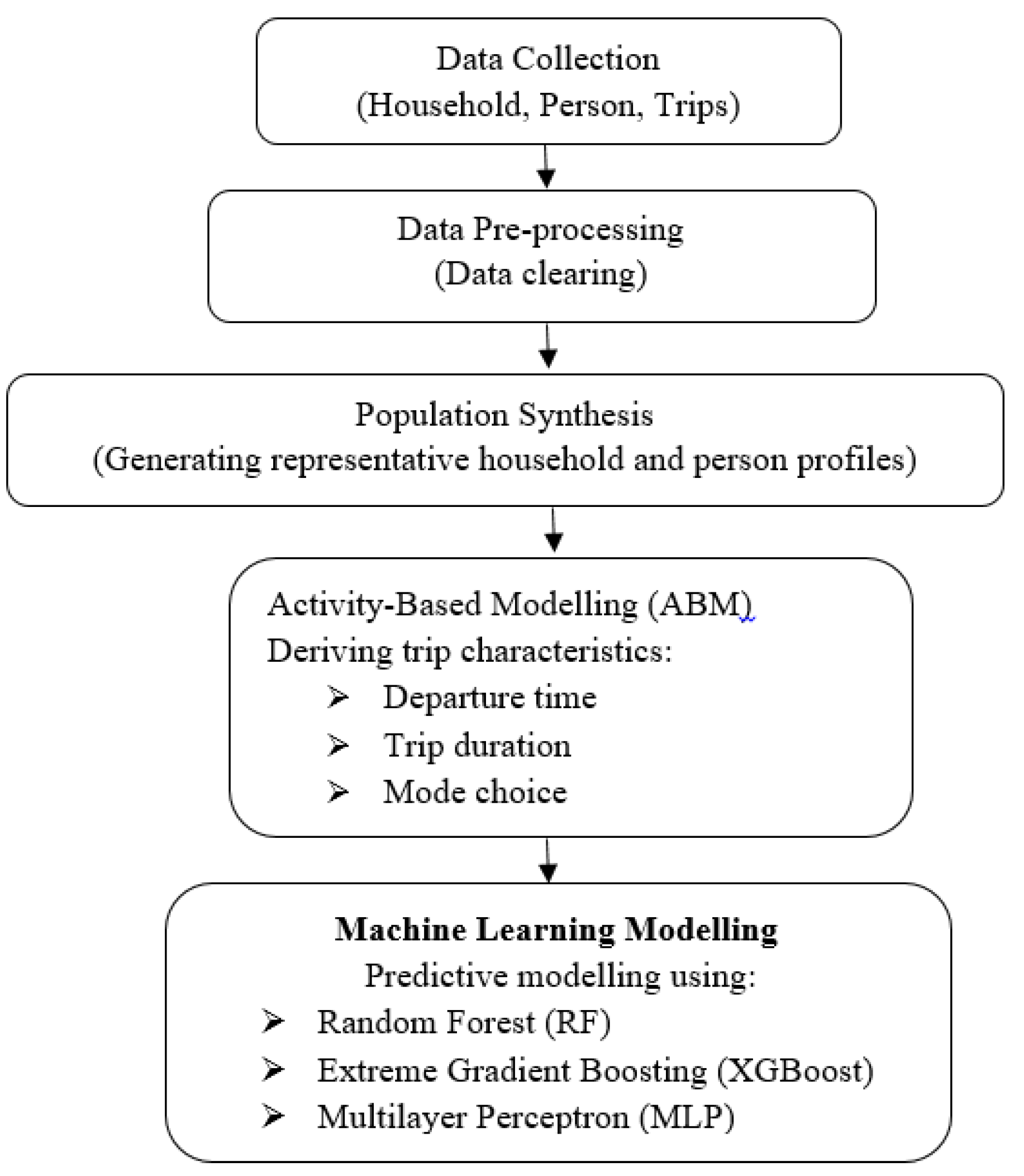
3.2. Methodology
In this study, as outlined in the methodological framework, we integrated ABM with machine learning techniques to provide a broad understanding of travel behaviour. The ABM approach analyses trips and their related activities and captures the full spectrum of daily activity-travel patterns. This helps to analyse departure times, trip chaining, travel durations, and mode choices that occur within 24 hours. Primary data i.e., household survey data, was collected, considering information on travel patterns, socio-economic characteristics, and activity schedules. As a complement for the data, secondary data was collected from Bahir Dar city municipality, and demographic statistics and census information were gained from there. Including the city centre and Abay Mado, the study area was divided into 18 Traffic Analysis Zones (TAZ). The analytical procedure contains population synthesis, ABM, and machine learning analysis. Each of them are discussed in the sections below.
3.2.1. Population Synthesis
To generate a synthetic population, we used an open-source platform, PopulationSim. To ensure representativeness, the sample data collected through the survey were expanded using marginal distributions from census data. This synthesized population was then used as the foundation for ABM simulation.
3.2.2. Activity-Based Modeling
PTV VISUM software was used to simulate travel demand and activity-travel interactions as well try to generate activities, tours and trips. This platform supports large-scale network analysis and integrates ABM principles with advanced traffic assignment algorithms.
3.2.3. Machine Learning Analysis
To enhance predictive accuracy and uncover hidden behavioural patterns, machine learning models were applied using Python (Pandas, Scikit-learn, and TensorFlow libraries) within the Jupyter Notebook environment. Specifically, Random Forest, Extreme Gradient Boosting (XGBoost), and Multilayer Perceptron (MLP) models were implemented to predict trip durations and analyze peak-hour dynamics. These models enabled identification of key factors affecting travel times and improved understanding of the temporal patterns in travel behavior.
Figure 2.
Methodological framework.
3.3. Machine Learning Parameter Settings
The three ML models, i.e., RF, XGBoost, and MLP, were applied to model trip durations. These models were trained with different hyperparameters for balancing accuracy and computational efficiency. RF was trained with 300 estimators, XGBoost similarly with 300 estimators, with a maximum depth of 5 and a learning rate of 0.1. The MLP was designed with two hidden layers (64 and 32 neurons) and with a maximum of 1000 iterations.
4. Data Analysis
In this section, try to present data found from Primary data that obtained from household surveys, focusing on individual-level information, including travel and socio-economic data, using a questionnaire.

Table 1.
Number of persons, households, car ownership, trips and before and after population synthesis.
Table 1.
Number of persons, households, car ownership, trips and before and after population synthesis.
| Before Population Synthesis | After Population Synthesis | |
| Number of Households | 1,014 | 14,457 |
| Number of Persons | 2,756 | 35,110 |
| Number of Cars | 268 | 3,934 |
| Total activity executions | 8,757 | 147,351 |
5. Model Results and Discussions
This section mainly covers the results and discussion on how departure times affect trip duration and mode choice. It examines and models the relationship between these factors using machine learning techniques, employing activity-based models (ABMs) with Visum software, following the population synthesis conducted with PopulationSim software. The analysis produced a total of 147,351 activity executions, 56,121 tours, and 112,429 trips.
5.1. Activity Profiles
The figure displayed below shows activity profiles generated from Visum software, illustrating the chronological sequence of various activities throughout the day. Individual activities are depicted on a time axis, with overlapping activities represented one above the other. This format allows the y-axis to indicate the number of simultaneous activities at any given time, as shown in the figure below.
In August 2023, the Ethiopian government declared a state of emergency in the Amhara region, including Bahir Dar, placing it under a military command post. This situation has significantly impacted the execution of activities and travel patterns in the city. Due to concerns related to safety and security, trips between 0:00-5:00 AM and 9:00 PM-11:59 PM are nearly non-existent. The data clearly reflect these patterns, with the majority of activity occurring during daytime hours.
Figure 5.
Activity profiles for various activities.
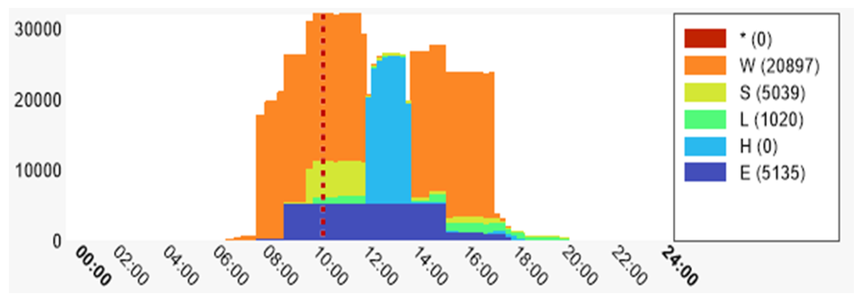
The vertical dotted line at 10:00 in the diagram serves as a reference point to highlight the distribution of activities occurring at that specific time. At 10:00, approximately 20,897 work activities (W) are shown in orange, 5,039 shopping activities (S) in yellow, 1,020 leisure activities (L) in green, and 5,135 educational activities (E) in blue. Home activities (H) are recorded as zero and are represented in light blue.
The diagram depicts the distribution of activities over 24 hours, divided into specific time intervals. There is almost no activity during the early morning, since it is resting time and due to restrictions imposed by the state of emergency. The morning peak, i.e., 06:30-08:30, shows a sharp rise due to work and educational activities. Around midday, i.e., 11:30-13:30, it shows an increase in shopping and leisure activities, since it is lunch and rest time. The afternoon time, i.e., 13:30-16:00, again is dominated by work, and school activities decline gradually. At 16:00-17:00, there is a visible transition to leisure, since this time is when individuals finish their work and school activities and return home. At the start of the evening, i.e., 17:00-20:00, although there are declines, leisure activities still remain, and some shopping occurs. With the last period, i.e., 20:00-24:00, all activities stop since it is night or rest time, and this is also due to restrictions by the command post.
From the figure, we can conclude that work and educational activities take up the most time of the day. Following these two, leisure and shopping take the next level, which mostly peak at midday and afternoon hours. Home activities mainly occur at the morning and evening. This structured pattern demonstrates how societal routines and contextual factors, such as security restrictions, shape the rhythm of daily activity execution.
5.2. Distribution of Activity Execution by Type, Comparing at Abay Mado and Toward City Centre
Figure 6 shows the distribution of different types of activities carried out at Abay Mado and Gabiya. The activity categories are presented on the x-axis, while their frequencies are displayed on the y-axis. The percentages above the bars provide a quick comparison of the share of each activity between the two locations. The results highlight distinct differences between the areas. Work-related activities (W) are overwhelmingly concentrated in Gabiya, reflecting its role as the primary employment hub. Shopping (S) is also more common in Gabiya, underlining its importance as a commercial center. Abay Mado, on the other hand, stands out for education-related activities (E), accounting for nearly three-quarters of the total, and also hosts the majority of leisure (L) activities. Leisure is the least frequent activity overall, but Abay Mado records a larger share compared to Gabiya. Generally, the results show that Gabiya is mostly shaped by economic activities and Abay Mado is more strongly connected to education and community life.
5.3. Distribution of Trip Durations
The histogram and kernel density estimation plot of trip durations is illustrated in Figure 7. It shows that with peaks around 2.5 to 7.5 minutes, most trips are relatively short. After 10 minutes, the frequency of trips decreases sharply, which indicates that longer trips are not frequent. Minibus trips extend up to 20 minutes while serving medium-length trips, whereas walking, auto-rickshaw, and car trips peak within 3-8 minutes. Bus trips dominate the longer durations, reaching 40–50 minutes, but their wide variability indicates reliability issues.
5.4. Proportion of Trips Across Different Modes
The proportion of trips across different modes is illustrated in Figure 8 below. The result shows and it shows minibuses take a higher proportion of urban mobility, especially during peak hours, i.e., around 8AM, 12 PM, 1 PM, 2PM and 5 PM. Auto-rickshaws also take a larger proportion of trips during these times. However, buses, cars, and walking show fewer frequent trips when compared with the two. From these, we can conclude that during the periods with high travel demand, minibuses and slightly auto-rickshaws play a crucial role in meeting short to medium distance mobility needs.
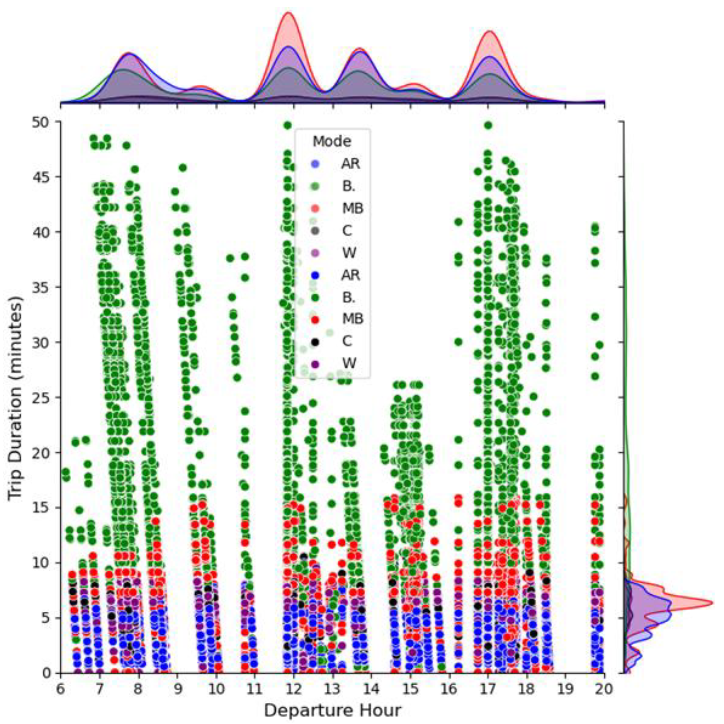
5.5. Actual Trip Duration vs. Departure Time by Mode
The relationship between departure time and trip duration is shown in Figure 9 below, and each point is coloured by transport mode. At the top of the figure, there are density plots to show the time when most trips take place, and this makes it easy to identify peak travel periods. The overall visualization clearly shows the time when trips are most common, and how long they will likely last depending on the mode of transport. This can also highlight that all modes may not respond to traffic similarly. At the peak travel hours, i.e., 8 AM, 12 PM, 1 PM, and 5 PM, buses and minibuses display the widest variation in travel times. This can show that the modes become more vulnerable to delays by the effects of congestion, high passenger demand, and frequent stops. When we see the cars and auto-rickshaws, they can show more reliable travel times, since they have narrower spreads in trip durations across the day. On the other hand, walking trips remain fixed every time without being affected by traffic conditions. Generally, from the result, we can conclude that buses and minibuses are heavily burdened with peak-hour pressures, and private and non-motorized modes stay in a more stable state throughout the day.
5.6. Model Performance on Trip Duration Prediction
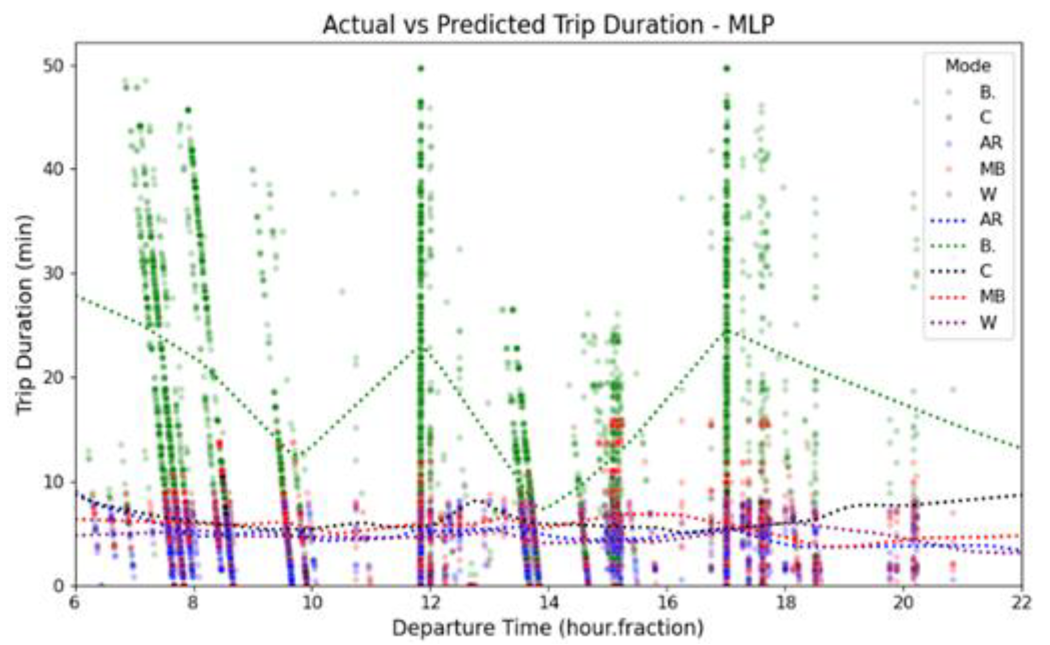
Figure 10, 11, and 12 show trip duration predictions by departure time for RF, XGBoost, and MLP, respectively. All models capture the daily travel rhythm with clearly visible peaks around 8 AM, 12 PM, 1 PM, and 5 PM. The RF model can align the observed trends with the peaks and troughs in trip duration, since it closely replicates the observed trends. Although the XGBoost model shows greater fluctuations, it can similarly show similar patterns with RF. The third model, MLP, has relatively higher variability, and it often deviates from the observed patterns. This is highly visible, especially at the time of longer trips, around 1:00 PM and 5:00 PM peaks. From the results, we can clearly understand that decision tree-based ensemble models (RF and XGBoost) can represent time-dependent trip durations more stably and accurately than the neural network approach.
Figure 10.
Actual vs. predicted trip duration using random forest.
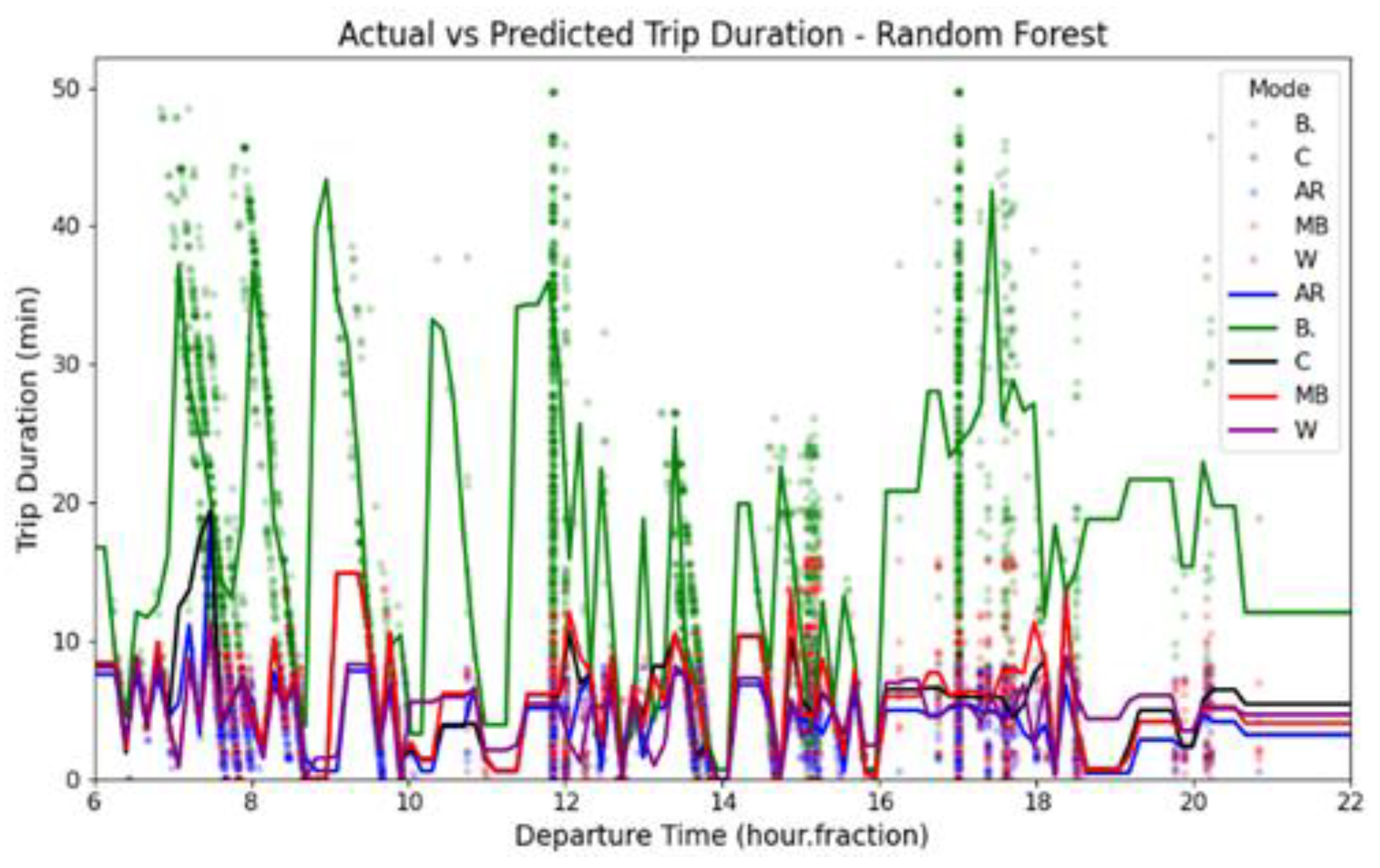
Figure 11.
Actual vs. predicted trip duration using XGBoost.
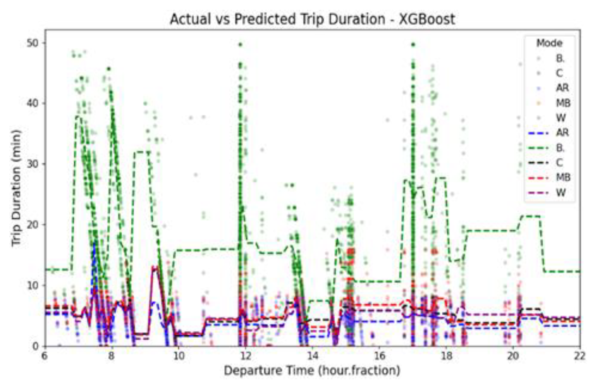
Figure 12.
Actual vs. predicted using MLP.
5.7. Model Validation (Actual vs Predicted Trip Duration)
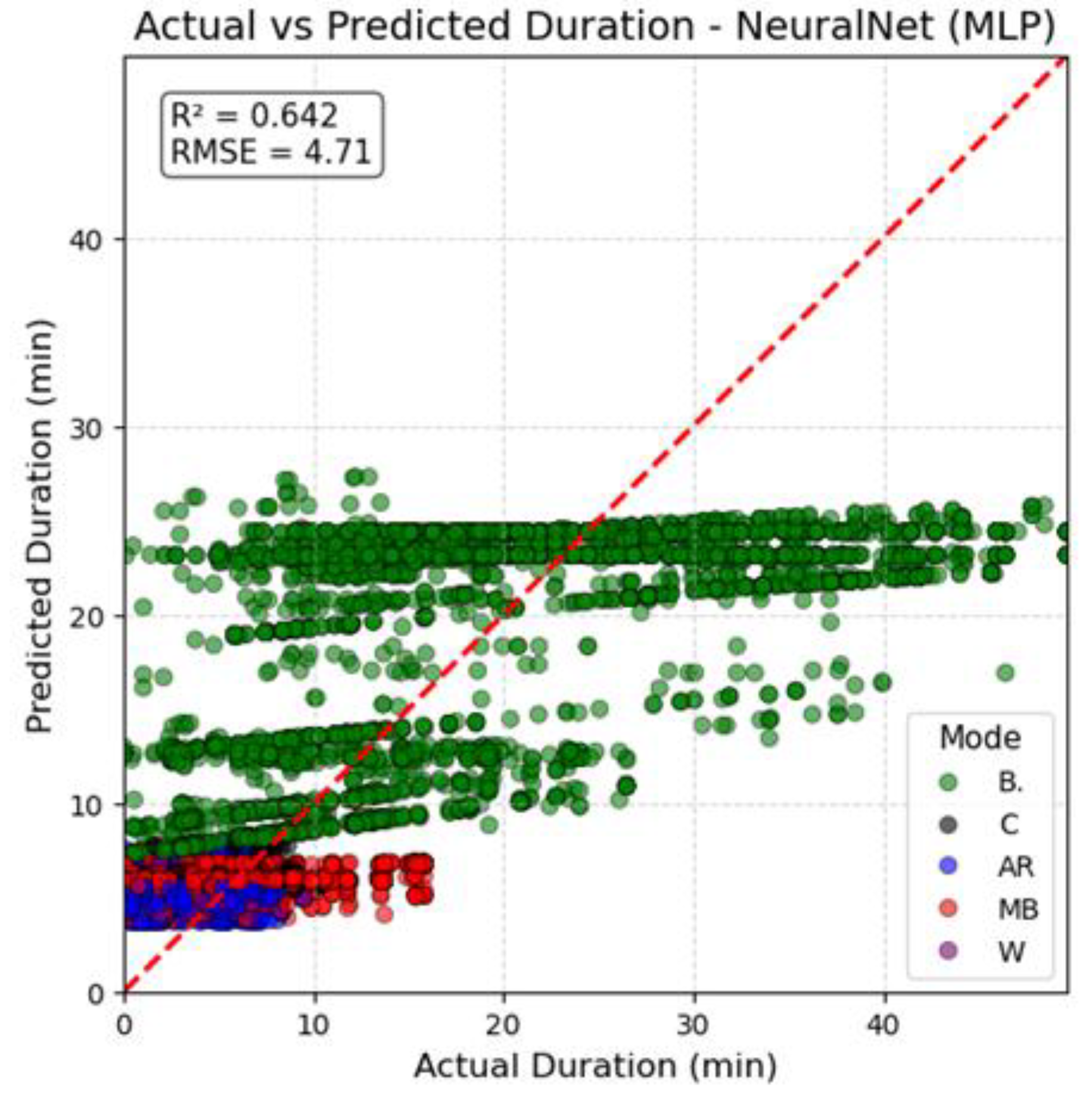
The figure below presents the comparison between actual and predicted trip durations for Random Forest, XGBoost, and MLP models. The result of the RF model shows the best performance compared with other models, and it has R² = 0.769 and RMSE = 3.78. Next to RF, the XGBoost model is the other model with better performance results, i.e., R² = 0.756, RMSE = 3.89 and the last model, MLP, has a lower performance than the other models, i.e., R² = 0.642, RMSE = 4.71. In both Random Forest and XGBoost, predictions cluster closely around the 45° diagonal line, confirming high predictive reliability, particularly for short and medium trips. Across all models, higher variability is observed in bus and minibus trips, whereas car, walking, and auto-rickshaw trips remain relatively consistent and predictable.
Figure 12.
comparison between actual and predicted trip durations for random forest.
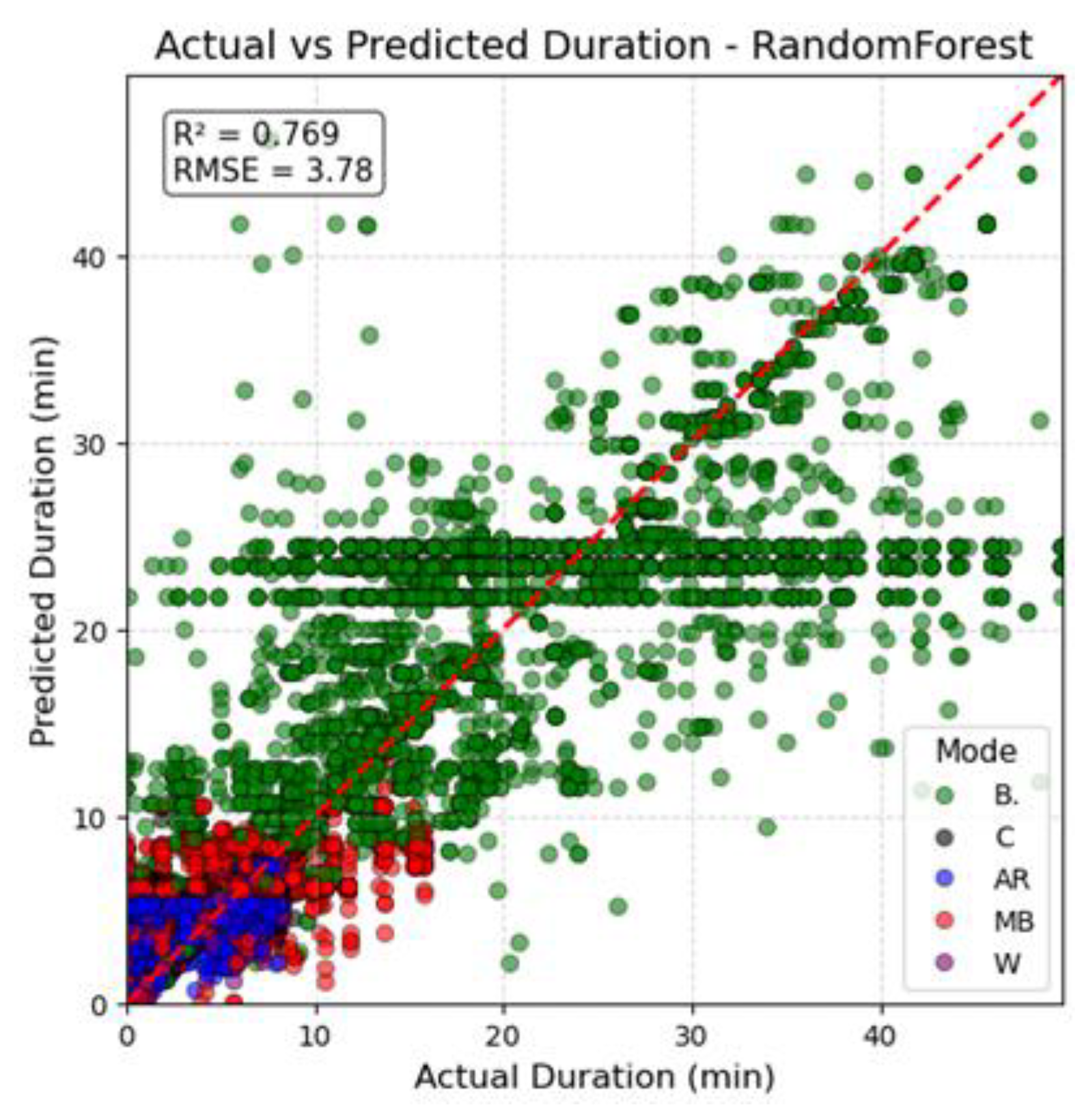
Figure 13.
comparison between actual and predicted trip durations for XGBoost.

Figure 14.
comparison between actual and predicted trip durations for MLP.
6. Conclusions
This study demonstrates that departure time plays a pivotal role in influencing both trip duration and mode choice in Bahir Dar City. Activity-based modeling revealed strong spatial and temporal variations in travel demand, with the city centre acting as the dominant attractor for work-related activities, resulting in pronounced morning, midday and evening peak periods. From the trip duration analysis, the buses and minibuses are highly sensitive to congestion and peak-hour demand. This leads to higher variability in time or lower reliability, but cars, auto-rickshaws, and walking maintain more consistent travel times. In addition, in accommodating daily mobility needs, mode share analysis shows that minibuses are dominant by getting supported by auto-rickshaws.
Machine learning models reinforced these findings, with Random Forest emerging as the most reliable predictor of trip durations across departure times, outperforming XGBoost and MLP. The prediction result of RF is highly related to the observed data, and this shows the importance of ensemble methods for modelling complex urban travel behaviors.
Generally, the results in the study highlighted new evidence on the interactions between departure time, mode choice, and trip duration, and provided actionable insights for policymakers and urban planners. Enhancing the efficiency of minibuses and buses during peak hours, diversifying modal options, and implementing demand management strategies could significantly reduce congestion and improve mobility reliability. This study also highlights the need for future work that explores the influence of land use on travel behavior, to address the uneven distribution of demand, improve travel time reliability, and enhance the predictive accuracy of urban mobility models.
Author Contributions
Conceptualization, T.K.A.; methodology, T.K.A.; software, T.K.A.; formal analysis, T.K.A.; data curation, T.K.A.; writing—original draft preparation, T.K.A.; supervision, J.J., M.D.Y., Y.M., A.A., and G.S.; project administration, J.J.; writing—review and editing, J.J., M.D.Y., Y.M., A.A., and G.S. All authors have read and agreed to the published version of the manuscript and are accountable for all aspects of the work.
Institutional Review Board Statement
This study was reviewed and approved by the Bahir Dar Institute of technology Institutional Research Review board, under approval number BiT-IRERB/053/2025. The procedures followed were in accordance with the ethical standards of the responsible committee on human experimentation and with the Helsinki Declaration of 1975, as revised in 2013.
Informed Consent Statement
Written informed consent was obtained from all study participants during the survey. Participants were fully informed about the objectives of the study, the voluntary nature of their participation, their right to withdraw at any time, and the confidentiality of the information collected.
Data Availability Statement
The data presented in this study are available on request from the corresponding author.
Acknowledgments
The authors gratefully acknowledge the support of Bahir Dar Institute of Technology, Bahir Dar University, for providing the necessary facilities and resources to conduct this research. Special thanks are extended to Bahir Dar Municipality and Bahir dar traffic office for providing access to essential data that supported this study. Finally, we thank colleagues and reviewers for their constructive feedback and valuable suggestions, which helped improve the quality of this manuscript.
Conflicts of Interest
The authors declare no conflicts of interest.
References
- R. Moeckel et al., “The Activity-based model ABIT: Modeling 24 hours, 7 days a week,” Transp. Res. Procedia, vol. 78, no. Ewgt 2023, pp. 499–506, 2024. [CrossRef]
- N. A. Nguyen, J. Schweizer, and F. Rupi, “Large-scale activity-based demand generation modeling: A literature review and exploration of potential approaches,” Transp. Eng., vol. 20, no. December 2024, p. 100329, 2025. [CrossRef]
- D. Wang and T. Cheng, “A spatio-temporal data model for activity-based transport demand modelling,” Int. J. Geogr. Inf. Sci., vol. 15, no. 6, pp. 561–585, 2001. [CrossRef]
- S. Cho, “Modeling Daily Travel Choices in an Activity- based Framework considering Spatiotemporal Constraints,” pp. 1–15, 2023. [CrossRef]
- Y. Delhoum, R. Belaroussi, F. Dupin, and M. Zargayouna, “Activity-based demand modeling for a future urban district,” Sustain., vol. 12, no. 14, 2020. [CrossRef]
- C. Bhat and F. S. Koppelman, “A retrospective and prospective survey of time-use research,” no. March, 2014. [CrossRef]
- K. M. Kockelman, “Travel behavior as function of accessibility, land use mixing, and land use balance: Evidence from San Francisco Bay Area,” Transp. Res. Rec., no. 1607, pp. 116–125, 1997. [CrossRef]
- K. Salazar-Serna, L. Cadavid, and C. J. Franco, “Analyzing Transport Policies in Developing Countries With Abm,” Simul. Ser., vol. 56, no. 1, pp. 651–657, 2024. [CrossRef]
- F. Orsi and D. Geneletti, “Transportation as a protected area management tool: An agent-based model to assess the effect of travel mode choices on hiker movements,” Comput. Environ. Urban Syst., vol. 60, pp. 12–22, 2016. [CrossRef]
- G. R. A. Lekshmi, V. S. Landge, and V. S. S. Kumar, “Activity Based Travel Demand Modeling of Thiruvananthapuram Urban Area,” Transp. Res. Procedia, vol. 17, no. 14, pp. 498–505, 2016. [CrossRef]
- W. W. Recker, “A bridge between travel demand modeling and activity-based travel analysis,” Transp. Res. Part B Methodol., vol. 35, no. 5, pp. 481–506, 2001. [CrossRef]
- S. Rasouli and H. Timmermans, “Activity-based models of travel demand: Promises, progress and prospects,” Int. J. Urban Sci., vol. 18, no. 1, pp. 31–60, 2014. [CrossRef]
- S. Nayak and D. Pandit, “A critical review of activity participation decision: a key component of activity-based travel demand models,” Int. J. Urban Sci., vol. 27, no. 4, pp. 670–703, 2023. [CrossRef]
- M. H. Hafezi, L. Liu, and H. Millward, “A time-use activity-pattern recognition model for activity-based travel demand modeling,” Transportation (Amst)., vol. 46, no. 4, pp. 1369–1394, 2019. [CrossRef]
- K. M. K. Atousa Tajaddini, Geoffrey Rose and and H. L. Vu, “Recent Progress in Activity-Based Travel Demand Modeling: Rising Data and Applicability,” Intech, vol. i, no. tourism, p. 13, 2012. [CrossRef]
- W. Davidson, P. Vovsha, J. Freedman, and R. Donnelly, “CT-RAMP Family of Activity-Based Models,” no. January 2010, 2016.
- A. A. Abdullah, N. S. Mohammed, M. Khanzadi, and M. Safar, “A Comprehensive Review of Machine Learning Approaches : Techniques, Applications, and Trends Abdulhady Abas Abdullah Artificial Intelligence and Innovation Centre, University of Computer Science, Faculty of Science, Soran University Health Informatio,” no. February, 2025. [CrossRef]
- A. N. P. Koushik, M. Manoj, and N. Nezamuddin, “Machine learning applications in activity-travel behaviour research: a review,” Transp. Rev., vol. 40, no. 3, pp. 288–311, 2020. [CrossRef]
- M. M. Hassan et al., “A comparative assessment of machine learning algorithms with the Least Absolute Shrinkage and Selection Operator for breast cancer detection and prediction,” Decis. Anal. J., vol. 7, no. April, p. 100245, 2023. [CrossRef]
- A. A. Khan, O. Chaudhari, and R. Chandra, “A review of ensemble learning and data augmentation models for class imbalanced problems: Combination, implementation and evaluation,” Expert Syst. Appl., vol. 244, no. November 2023, p. 122778, 2024. [CrossRef]
- K. Worden, W. J. Staszewski, and J. J. Hensman, “Natural computing for mechanical systems research: A tutorial overview,” Mech. Syst. Signal Process., vol. 25, no. 1, pp. 4–111, 2011. [CrossRef]
- G. N. Bifulco, A. Cartenì, and A. Papola, “An activity-based approach for complex travel behaviour modelling,” Eur. Transp. Res. Rev., vol. 2, no. 4, pp. 209–221, 2010. [CrossRef]
- J. L. Bowman and M. E. Ben-Akiva, “Activity-based disaggregate travel demand model system with activity schedules,” Transp. Res. Part A Policy Pract., vol. 35, no. 1, pp. 1–28, 2001. [CrossRef]
- H. Behrooz and Y. M. Hayeri, “Machine Learning Applications in Surface Transportation Systems: A Literature Review,” Appl. Sci., vol. 12, no. 18, 2022. [CrossRef]
- W. F. Admasu, A. Boerema, J. Nyssen, A. S. Minale, E. A. Tsegaye, and S. Van Passel, “Uncovering ecosystem services of expropriated land: The case of urban expansion in bahir dar, northwest ethiopia,” Land, vol. 9, no. 10, pp. 1–20, 2020. [CrossRef]
Figure 3.
Random forest architecture .
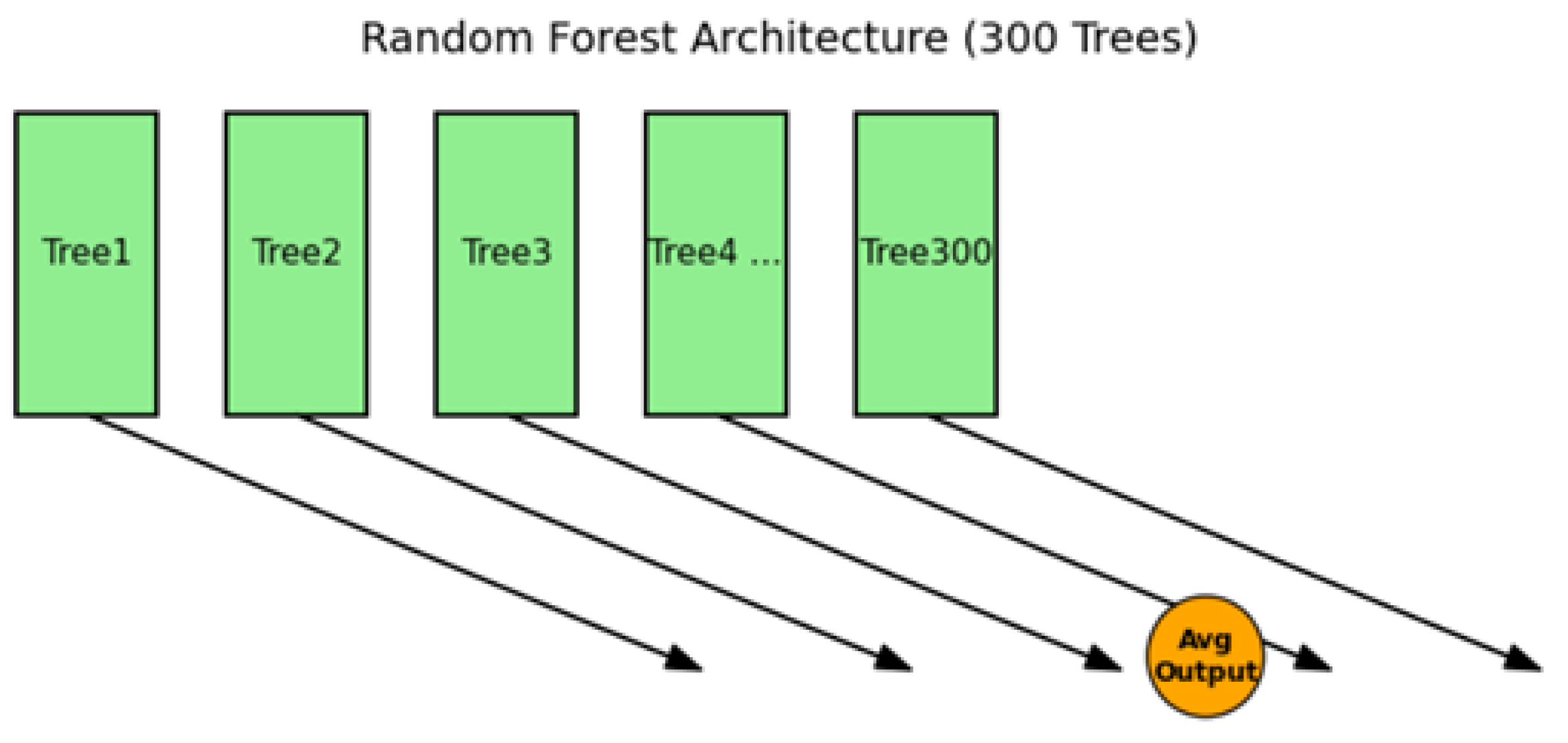
Figure 4.
XGBoost architecture.
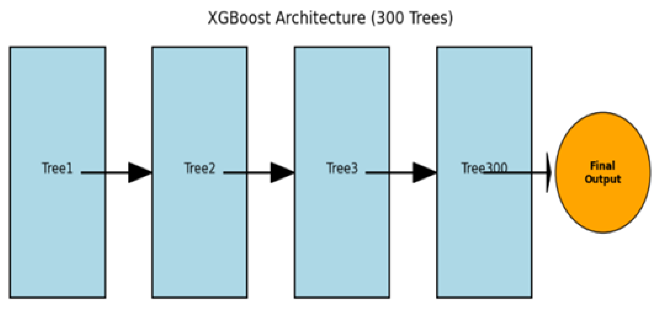
Figure 5.
Multilayer Perceptron (MLP) architectural diagram.
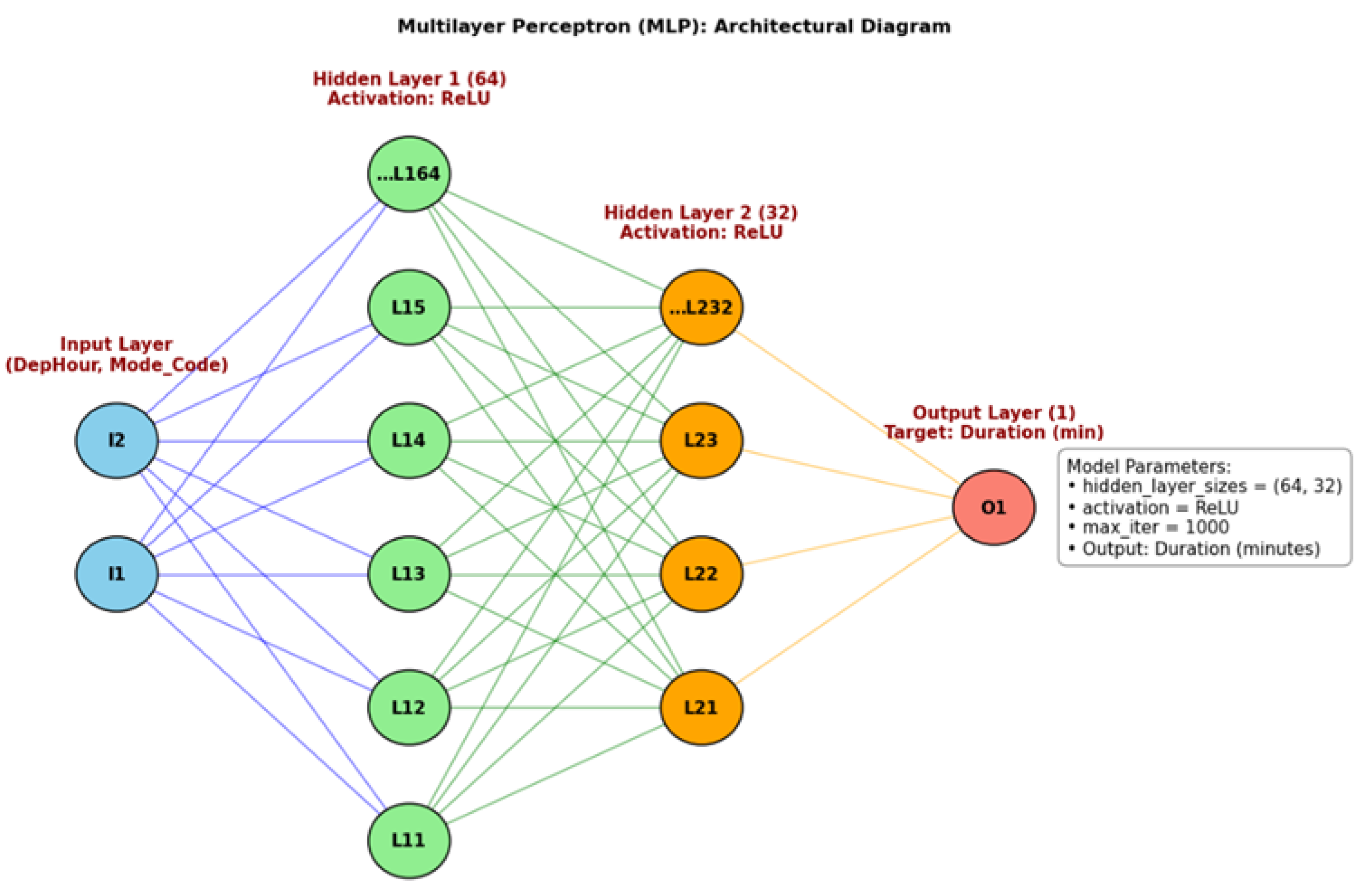
Figure 6.
Distribution of activity execution by type, comparing at Abay Mado and towards City Centre.
Figure 6.
Distribution of activity execution by type, comparing at Abay Mado and towards City Centre.
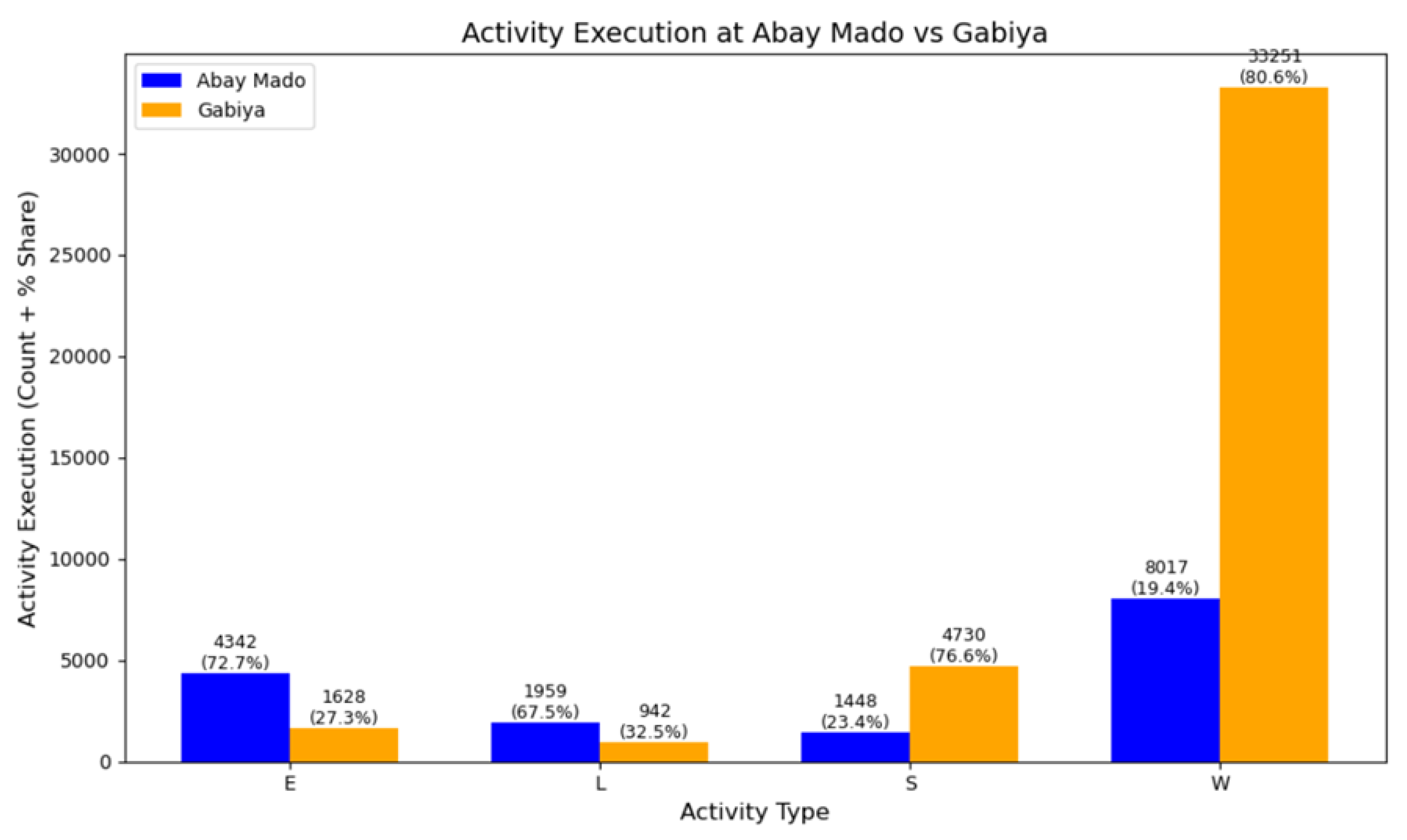
Figure 7.
Distribution of trip durations by mode.
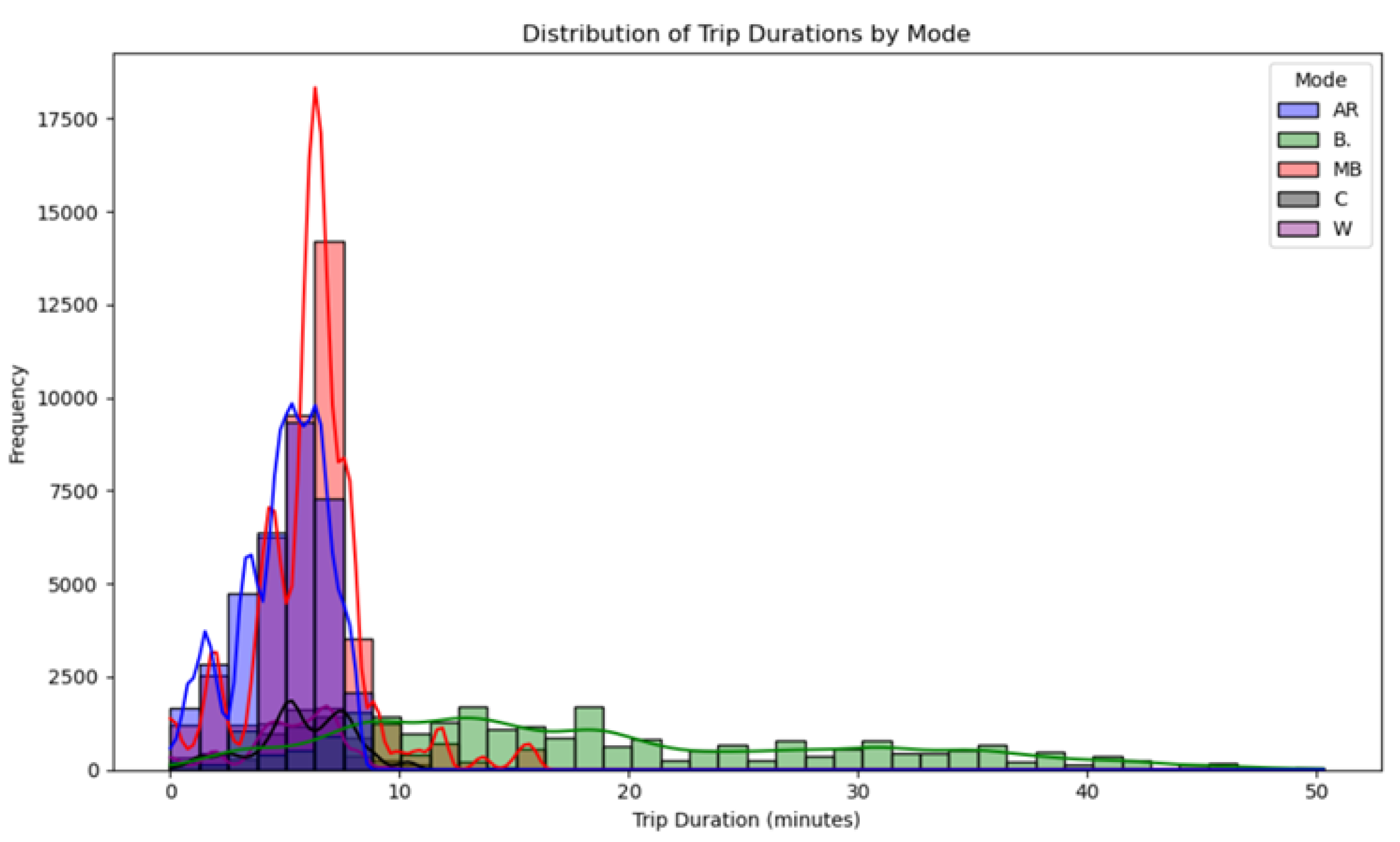
Figure 8.
proportion of trips across different modes.
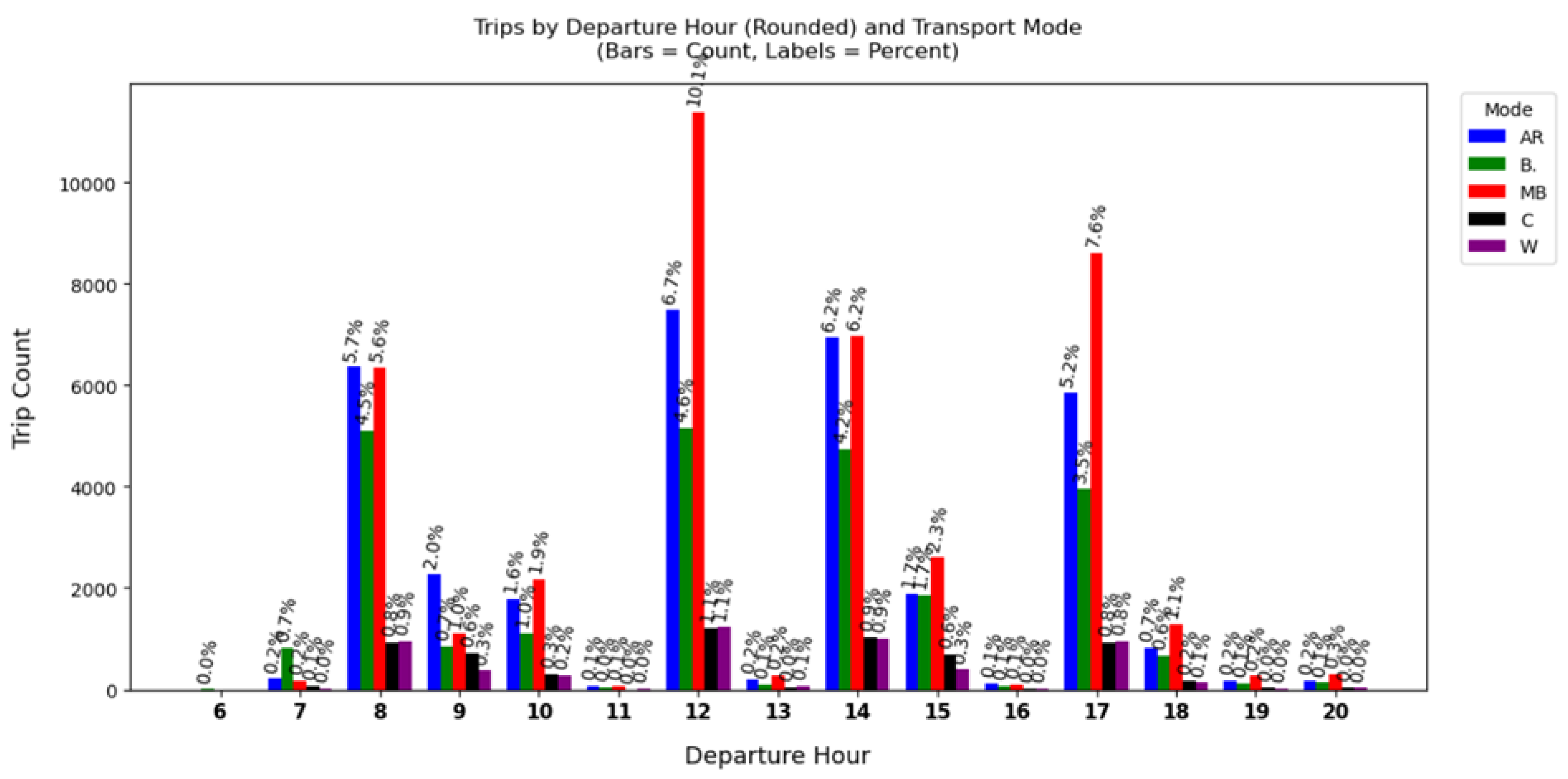
Figure 9.
Relationship between departure time and trip duration, by modes.
Disclaimer/Publisher’s Note: The statements, opinions and data contained in all publications are solely those of the individual author(s) and contributor(s) and not of MDPI and/or the editor(s). MDPI and/or the editor(s) disclaim responsibility for any injury to people or property resulting from any ideas, methods, instructions or products referred to in the content. |
© 2025 by the authors. Licensee MDPI, Basel, Switzerland. This article is an open access article distributed under the terms and conditions of the Creative Commons Attribution (CC BY) license (http://creativecommons.org/licenses/by/4.0/).
Copyright: This open access article is published under a Creative Commons CC BY 4.0 license, which permit the free download, distribution, and reuse, provided that the author and preprint are cited in any reuse.


