
Submitted:
25 September 2025
Posted:
29 September 2025
You are already at the latest version
Abstract
This work constructs a new mathematical model for the vibrations of a Bernoulli beam that can come in contact with a reactive obstacle situated below its right end. The obstacle reaction is described by the Damped Normal Compliance (DNC) contact condition. This condition takes into account the energy dissipation during the contact process. The steady states of the
model are described and the model is studied computationally for different values of obstacle stiffness and damping. The numerical simulations illustrate how the beam’s end penetration and vibrations differ in soft vs. stiff obstacle environments, and how damping modifies the dynamic behavior. The results may be useful for vibration control and material interaction in settings when collisions or repetitive contacts occur. By providing computational and analytical insights, the study is an addition to the Mathematical Theory of Contact Mechanics.
Keywords:
dynamic contact
; damped normal compliance (DNC)
; vibrating Bernoulli beam
; obstacle problem
; simulations
1. Introduction
The interaction of vibrating structures via contact with other system parts and components is an important topic in mechanical and structural engineering, with applications ranging from robotics, transportation, automotive, to aerospace systems and MEMS. When a beam repeatedly strikes an obstacle, its dynamic response is governed in part by the condition used to describe the contact process. Classical contact or impact models, such as the Hertz condition, often assume rigid, instantaneous contact with a restitution coefficient, but such models fail to capture the finite stiffness and energy dissipation observed in real materials; see e.g., [1,2], for the mathematical aspects. For this reason, the normal compliance condition was introduced in [3,4,5]. The normal compliance condition introduces a finite stiffness that allows small penetrations; however, without damping, they still underestimate energy losses during collisions [6]. To address these shortcomings, the damped normal compliance (DNC) law has recently been proposed that augments the normal compliance contact law with a damping term [7]. This modification yields a more realistic contact boundary condition because it permits controlled penetration while explicitly accounting for energy loss or dissipation during the process and thus is likely to improve the agreement with experiments.
The present study uses the DNC condition to model the contact between a vibrating Bernoulli beam and a reactive obstacle located below its free end. Such settings can be found in many MEMS systems, in actuators and grippers. We construct a new partial differential equation model that incorporates beam bending, and the contact boundary conditions of elastic compliance of the obstacle and damping. The main interest here is to study the effects of the beam’s flexural stiffness, the obstacle’s stiffness and its damping on the vibrations amplitude and frequencies of the beam. This may shed more light into the various noise characteristics of such systems. We note that the obstacle problem for the Gao beam has been stydied in [8] where the normal compliance contact condition was used.
The rest of the article is structured as follows. Section 2 describes in detail the setting and constructs the classical mathematical model, with the usual 4th order beam equation. In particular, it concentrates on the new DNC contact condition at the right end of the beam where the obstacle is situated. Energy considerations can be found in Section 3, where the energy balance is derived. Section 4 studies the steady states of the system. The condition on the force f, the position of the obstacle , and the beams stiffness , for existence of contact is obtained. Section 5 describes shortly, in Theorem 5.1 the existence of weak solutions to the model, presented in [9].
To explore the system dynamics numerically, we construct an implicit finite difference algorithm in Section 6. Numerical simulations reported in Section 7 illustrate how different combinations of obstacle stiffness and damping affect beam penetration, vibrations, and return to equilibrium. For very stiff obstacles with small damping, the behavior approaches rigid Signorini contact with noticeable rebounds, whereas moderate stiffness and larger damping lead to deeper penetration and faster decay of oscillations. These computational experiments underscore the wide range of behaviors captured by the DNC law and highlight its ability to bridge between purely elastic and highly dissipative contacts [4,7]. The paper ends with Section 8, which presents a short summary, some conclusions, and some unresolved problems, which we consider worth further study.
2. The Setting and the Model
This section presents the setting and constructs a classical model for the process of contact between a vibrating Bernoulli beam and a reactive object or obstacle, which is situated below the right end of the beam. The setting is illustrated in Figure 1.
The system consists of a Bernoulli beam that in its reference configuration occupies the (scaled with L – the original length of the beam) interval . The beam’s displacement from this reference configuration is denoted by , scaled by L, chosen as positive when above the x-axis. The beam is acted upon by a distributed force . The right end of the beam, at , can come in contact with a reactive obstacle, marked in Figure 1 as `obstacle.’ The position of the obstacle is at , and it is where contact can take place. Our main interest lies in what happens during contact between the beam’s end and the obstacle. We denote partial derivatives with subscripts, so , etc. The force applied to the beam is such that the beam can press against the obstacle, possibly leading to repeated contact.
We turn to the classical formulation of the model for the process.
Model 1.
Given the force , the excitation , and the coefficients , all positive constants, find the displacement field , for , such that:
The initial displacement and the initial velocity are given functions satisfying the compatibility conditions , , and and then .
Here, u and x are scaled with L, and so is ; , is the density of the beam material, A is the cross-sectional area, is Young’s modulus (elasticity modulus), and I is the second moment of the area of the beam’s cross-section. The external force f is scaled with , so it is force per unit volume of the beam. In addition, denotes the negative part function, that is when and when .
Remark 1.
A note on the DNC contact condition, (1d), [4]. When there is no contact, , the traction or stress at is zero since the end is free. When there is contact, , the obstacle reaction is given by
where κ is the obstacle stiffness and β is its damping coefficient. Thus, the DNC condition explicitly takes into account the energy loss during contact. It is also noted that R may be positive or negative, although the stiffness term always positive, as it points up. However, since when the obstacle is soft (small κ), the damping is large (large β) and the velocity is large and in the upward direction, R may be negative. As we show below, the energy dissipation is always negative when the end is moving. Furthermore, is the depth of the penetration of the beam into the obstacle, when in contact.
For the sake of simplicity, we introduce the cutoff function
It vanishes when there is no contact and, therefore the obstacle resistance can be written concisely as
3. Energy Balance and Dissipation
We derive the energy balance in the system, assuming that the solutions are sufficiently smooth for the manipulations to make sense. We multiply (1a) with and integrate over , for . We deal with the different terms separately. The first term, after integration by parts, yields
Here, the kinetic energy, at time t, is given by
Next, we note that
We have, using (3),
Moreover, using the initial condition ,
Furthermore, using integration by parts and the boundary conditions and the facts that and , we obtain
We now define the potential energy, at time t, of the system as
Result 1.
The system energy balance,
The first term on the right describes the initial kinetic energy and the second term the initial elastic potential energy. The third term describes the energy supplied or removed by the applied force, the last term is the energy dissipated by the obstacle. It follows, since the last term is negative when the end is in motion and in contact, that the obstacle’s resistance dissipates energy from the system.
4. Steady States
This section studies the steady states of the system. We assume that the applied force f is a negative constant, since if then the end does not come into contact with the obstacle. The steady solutions, denoted by , are found by setting the time derivatives in (1b)–(1d) to zero. Thus, we obtain the following ODEs model:
Model 2.
Given the force , positive constants, find the displacement field , such that:
Integrating four times with respect to x gives the general polynomial solution for (7) and applying the boundary conditions in (8), we obtain
Applying the boundary conditions at , we have
hence
and
This implies that there are two cases to consider:
(i) No contact: When then , and we find . Therefore, in this case, the solution is
Evaluating this at , we find , therefore:
Result 2.
[No contact] The condition for no contact is
Then and the solution is just the usual one of a linear beam with a free right end, and is given in (13).
Physically, this means that the (scaled) force is insufficient to bend the beam enough to contact the obstacle, since the beam stiffness opposes it.
(ii) Contact: When , then , , and we find from (11) and (12) that
Then, after rearranging and some manipulations, we obtain
which depends on and . We note that , hence . Thus, with A given in (15), the solution of the steady problem when contact takes place is
In particular,
We conclude that in the case with contact, we have:
Result 3.
[Contact] Assume that
Then, there is contact between the beam and the obstacle and the steady solution is given in (16).
Physically, this means that the (scaled) force to the beam’s stiffness ratio is sufficient to bend the beam so it comes in contact with the obstacle.
Figure 2 shows the computed solutions of the steady states, using formulas (13) or (16), depending on the inequality (14). In the simulations and and a constant force f are used. The figure shows the steady bending of the beam for various values of the force, and contact is established when the force is close to .
It is found that under a constant distributed load and the DNC contact condition with stiffness and obstacle position , the beam deflection naturally divides into two cases characterized by
When there is no-contact, and the deflection of the free end is above the obstacle. When there is contact. Clearly, is when the end of the beam just touches the obstacle, without penetrating it.
5. Abstract Formulation and Existence
The detailed proof of the existence of a weak solution to the problem can be found in [9]. Here, we just provide a short description and state the main existence theorem. The proof is based on a sequence of regularized problems, and then passing to the limits. The main issue is that the boundary conditions for are not well defined when we only know that has values in . Also, the discontinuity of causes some difficulty. For mathematical reasons, we add viscosity to the beam equation in the form of , for small , which allows us to obtain better estimates.
We first consider a problem in which is regularized by replacing it with a piecewise linear Lipschitz approximation given by
for a small . Eventually, we pass to the limits .
We set the problem in terms of , and then
We use the notation , and let and , with the usual inner products and norms.
The classical formulation of the regularized problem is:
Find such that
Next, we set the problem in a variational form. The function space in which one expects to seek weak solutions is the Sobolev space.
and
For the time dependence on , we require: and .
Denote such a space by ,
We choose as a test function. Multiplying Equation (19) by and integrating on , using various manipulations, Green’s identities, and the boundary conditions, we obtain the following.
The weak or variational formulation of the problem with viscosity, Model (19)–(24), is the following:
Model 3.
Given , and positive constants , find , such that , and for every test function that satisfies , (25) holds, together with
and
As was noted in [9], we need to control the boundary term and hence, we introduce the truncation function.
Then, we replace the term with
which is bounded and Lipschitz continuous.
We have the following existence theorem, established in [9].
Theorem 1
([9]). There exists a variational solution u to Model 3 in which the term is truncated as , and is replaced with . The solution with is weaker.
The proof uses a fixed-point argument and some regularization. Then, sufficient estimates are obtained that allow us to consider the case without viscosity, that is, the case .
6. Finite Difference Algorithms
We use an implicit second-order finite-difference algorithm for the simulations of the problem. The beam is divided into M uniform length segments . The simulations are performed over the time interval , and the time step is given by . Let be the approximation of the solution at the node at time , that is, , for and . First, we note that, thanks to the initial conditions in Equation (1e), we have
Moreover, thanks to the Dirichlet boundary condition in Equation (1b), we have
For and , the implicit finite difference scheme is given by
Rearranging terms, and defining , we have
Equation (29) is used to construct a linear system at every time level which is solved to obtain the discrete solution at that level. We note that when , we have the ghost node, for which we use the boundary condition in Equation (1b). In particular, using a second-order approximation of the derivative, this boundary condition gives us
Therefore, the finite-difference scheme Equation (29) for becomes
We also note that when and when , there are two ghost nodes: and . Using the boundary condition in Equation (1c), we have
Thus, the finite difference scheme for becomes
The contact boundary condition Equation (1d) is taken into account depending on whether the beam had contact with the obstacle at the previous time or not. We have the following two cases:
-
No contact:Thus, in the case of no contact, the finite difference scheme is
-
Contact:Thus, in the case of no contact, the finite difference scheme is
The algorithm is as follows.
| Algorithm 1 Implicit finite difference scheme for the vibrating beam |
Initialization:
|
7. Simulations
The implicit finite difference Algorithm 1 was implemented in MATLAB, and the backslash function was used to solve the linear system. In all simulations , the beam length was , the final time was , and . Moreover, the force was taken as and . The obstacle was located at . In this section, we report some of the more interesting computer experiments. Typically, each simulation took about 10-15 seconds, running in MATLAB.
The following are example simulations for various obstacle stiffnesses, , and damping coefficients . Typically, in Figure 3 we show the position of the right end of the beam over time for different values of and . It is seen that, progressively, the penetration decreases, and substantially changes between the values and , in the latter case there is virtually no penetration.
Result 4.
We observe the following:
- For large () and small (, the contact process behaves similarly to that with a Signorini (rigid) contact condition: very little penetration, high contact force and repeated bounces when the initial energy is sufficient.
- For moderate stiffness (), one obtains a normal compliance-like penetration, with partial rebounds damped out, depending on the values of .
- For small () and large (, the obstacle effectively behaves like a “soft, dissipative" material, such as tissue, allowing for deeper penetration and higher energy dissipation.
These results confirm that the DNC law can model a whole spectrum of contact behaviors, bridging between purely elastic and purely dissipative extremes.
8. Conclusions and Unresolved Questions
This work studies the vibrations of a Bernoulli beam that can come into contact with an obstacle, which is situated under its right end. The contact process is described by the Damped Normal Compliance boundary condition. The model consists of the usual 4th-order dynamic beam equation, together with the initial and boundary conditions. The interest lies in the obstacle’s resistance R, (3), which includes stiffness and damping terms, and is active once the right end is in contact.
The system energy balance is derived in Section 3, showing that the system loses energy because of damping, once the beam is in contact. The steady states of the system are found in Section 4. It is found that the ratio , where
controls when there is contact. Indeed, when there is no contact in the steady state and when the beam is in contact. When the beam’s end just touches the obstacle. The variational formulation of the problem is provided in Section 5, that includes the functional setting. It is noted that the term needs a special treatment, since for the trace is not well defined. We circumvent this problem by considering regularized problems with viscosity, the solutions of which are sufficiently regular to allow for the trace to exist. The existence of the variational solutions to the regularized problems are stated in Theorem 5.1. Moreover, the solutions of the problem without viscosity are obtained as limits and can be found in the weaker space . The proofs can be found in [9].
A finite difference scheme and algorithm for the simulations of the problem can be found in Section 6. The algorithm is implicit, and special attention is paid to the discretized contact conditions. Section 7 provides the simulation results. It is found that for a sufficiently large force, the beam penetrates the obstacle. Then, depending on the stiffness and damping, the simulations indicate that when the stiffness decreases and the damping increases, the penetration increases and the dying out of the oscillations is faster. These are summarized in the Results 4.
These results confirm that the DNC law can model a whole spectrum of contact behaviors, bridging between purely elastic and purely dissipative extremes.
We turn to some unresolved problems. More simulations and a numerical study of the dependence of the frequencies of vibration on the beam rigidity and the obstacle stiffness may be of practical interest. The case when there are two obstacles, one above and the other below, is of interest, especially numerically, since the vibration frequencies of the beam depend on the beam’s rigidity and the stiffness of the obstacles.
Further analysis of the problem is of interest.
Another aspect that may be of interest is the possible addition of friction to the contact, so that when the beam’s end, when in contact, undergoes friction and frictional energy dissipation, [6,10,11,12].
8.1. Steady States – Numerical Solution
In addition to the explicit formulas for the steady states of the beam, we implemented a numerical method, based on the dynamic case above, and compared the numerical and the closed-form solutions, to estimate the numerical errors.
Steady states do not involve time, so we discretize the beam into M equal segments of length such that , and let denote the displacements at .
For interior points , we can approximate the fourth derivative by the standard central difference scheme. Thus the discretized equation for becomes
At the left end , and , so we use the second-order approximation of to be
But , which implies that .
Now, at the right end , we have
We approximate the third derivative with the second-order backwards difference as
Then, we apply the DNC condition:
Figure 4.
Comparing the steady state numerical solution for the beam without or with contact, for with the exact solution. The obstacle is at .
Figure 4.
Comparing the steady state numerical solution for the beam without or with contact, for with the exact solution. The obstacle is at .
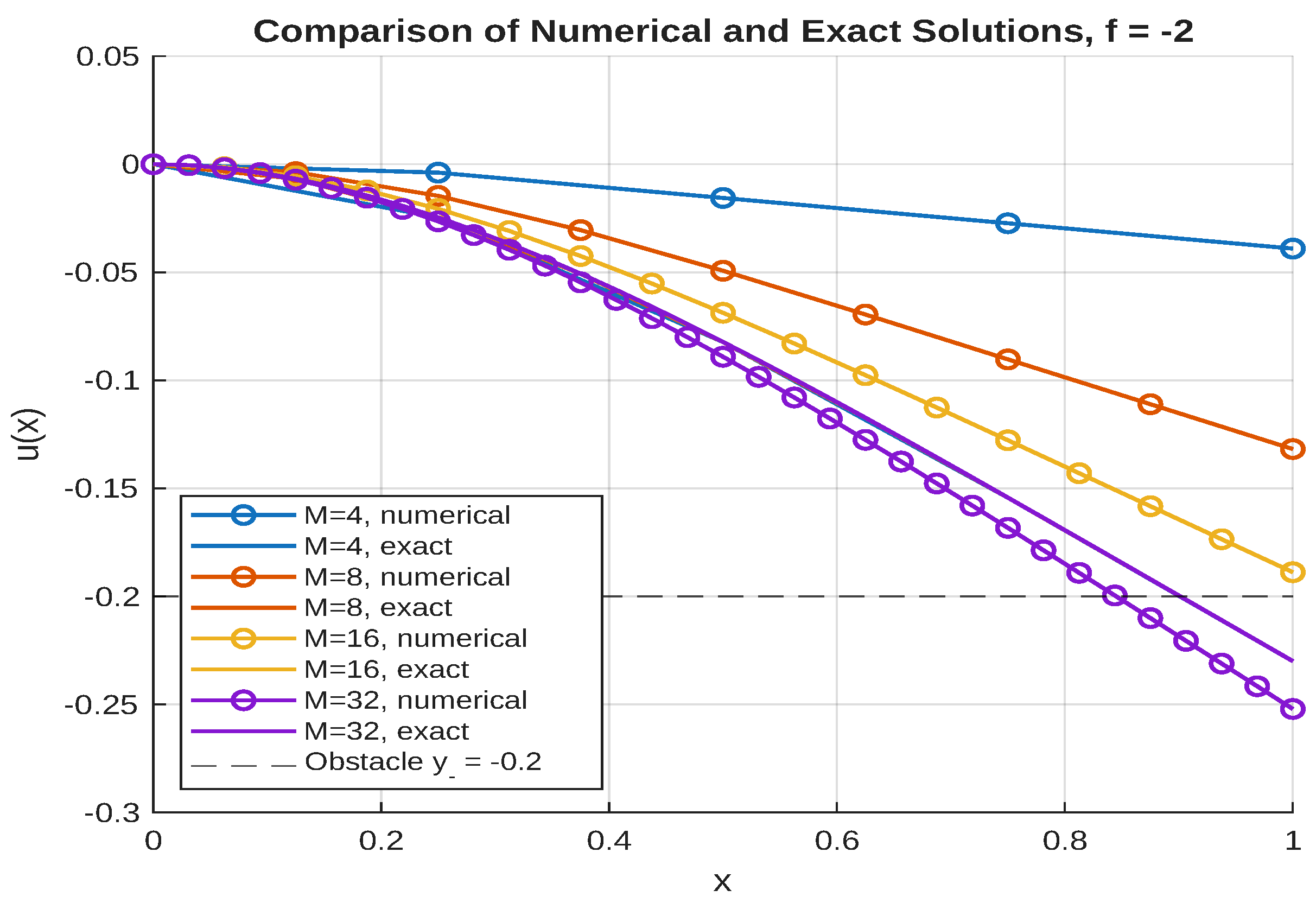
The following is the algorithm we used for the numerical solutions of the steady states. Comparison with the closed-form solution (13) or (16) provides confidence in our numerical simulations. Indeed, the comparison in Figure 3 shows numerical results that are very close to the closed-form results. Furthermore, Table 1 provides a more precise comparison, which is depicted in Figure 5.
| Algorithm 2 Case-Based Solver for the Steady-State Beam with DNC Condition |
|
The results of the numerical computations were found to be very close to those of the closed-form solutions, and are shown in Figure 3. Furthermore, the following table provided numerical comparison.
References
- Eck, C.; Jarusek, J.; Krbec, M. Unilateral contact problems: variational methods and existence theorems; CRC Press, 2005.
- Brogliato, B.; Ten Dam, A.; Paoli, L.; Ge not, F.; Abadie, M. Numerical simulation of finite dimensional multibody nonsmooth mechanical systems. Appl. Mech. Rev. 2002, 55, 107–150. [CrossRef]
- Oden, J.; Martins, J. Models and computational methods for dynamic friction phenomena. Computer methods in applied mechanics and engineering 1985, 52, 527–634. [CrossRef]
- Klarbring, A.; Mikelić, A.; Shillor, M. Frictional contact problems with normal compliance. International Journal of Engineering Science 1988, 26, 811–832. [CrossRef]
- Shillor, M.; Sofonea, M.; Telega, J.J. Models and analysis of quasistatic contact: variational methods; Vol. 655, Springer Science & Business Media, 2004.
- Kikuchi, N.; Oden, J.T. Contact problems in elasticity: a study of variational inequalities and finite element methods; SIAM, 1988.
- Shillor, M.; Pahuja, I. Damped Normal Compliance (DNC) and the restitution coefficient. Mathematics and Mechanics of Solids 2024, 29, 1627–1645.
- Andrews, K.; M’Bengue, M.; Shillor, M. Vibrations of a nonlinear dynamic beam between two stops. Discrete and Continuous Dynamical System (DCDS-B) 2009, 12, 23–38.
- Sosa Jones, G.; Shillor, M. A model for contact of a rod with an obstacle using the Damped Normal Compliance condition. Available at SSRN 4850822 2025.
- Duvant, G.; Lions, J.L. Inequalities in mechanics and physics; Vol. 219, Springer Science & Business Media, 2012.
- Simo, J.C.; Laursen, T. An augmented Lagrangian treatment of contact problems involving friction. Computers & Structures 1992, 42, 97–116. [CrossRef]
- Umer, M.; Gastaldi, C.; Botto, D. Friction damping and forced-response of vibrating structures: An insight into model validation. International Journal of Solids and Structures 2020, 202, 521–531. [CrossRef]
Figure 1.
The vibrating beam and the obstacle below the right end. Here u denotes the displacements; f the applied force; the obstacle is situated at below , where contact, which is described by the DNC condition, may take place.
Figure 1.
The vibrating beam and the obstacle below the right end. Here u denotes the displacements; f the applied force; the obstacle is situated at below , where contact, which is described by the DNC condition, may take place.
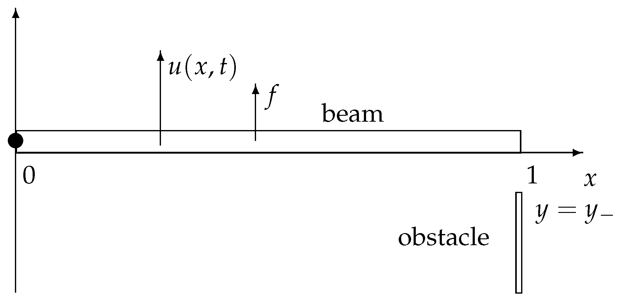
Figure 2.
Closed-form solutions (13) or (16) for different values of the force f. The obstacle at is at position . The force below leads to contact. Here, .
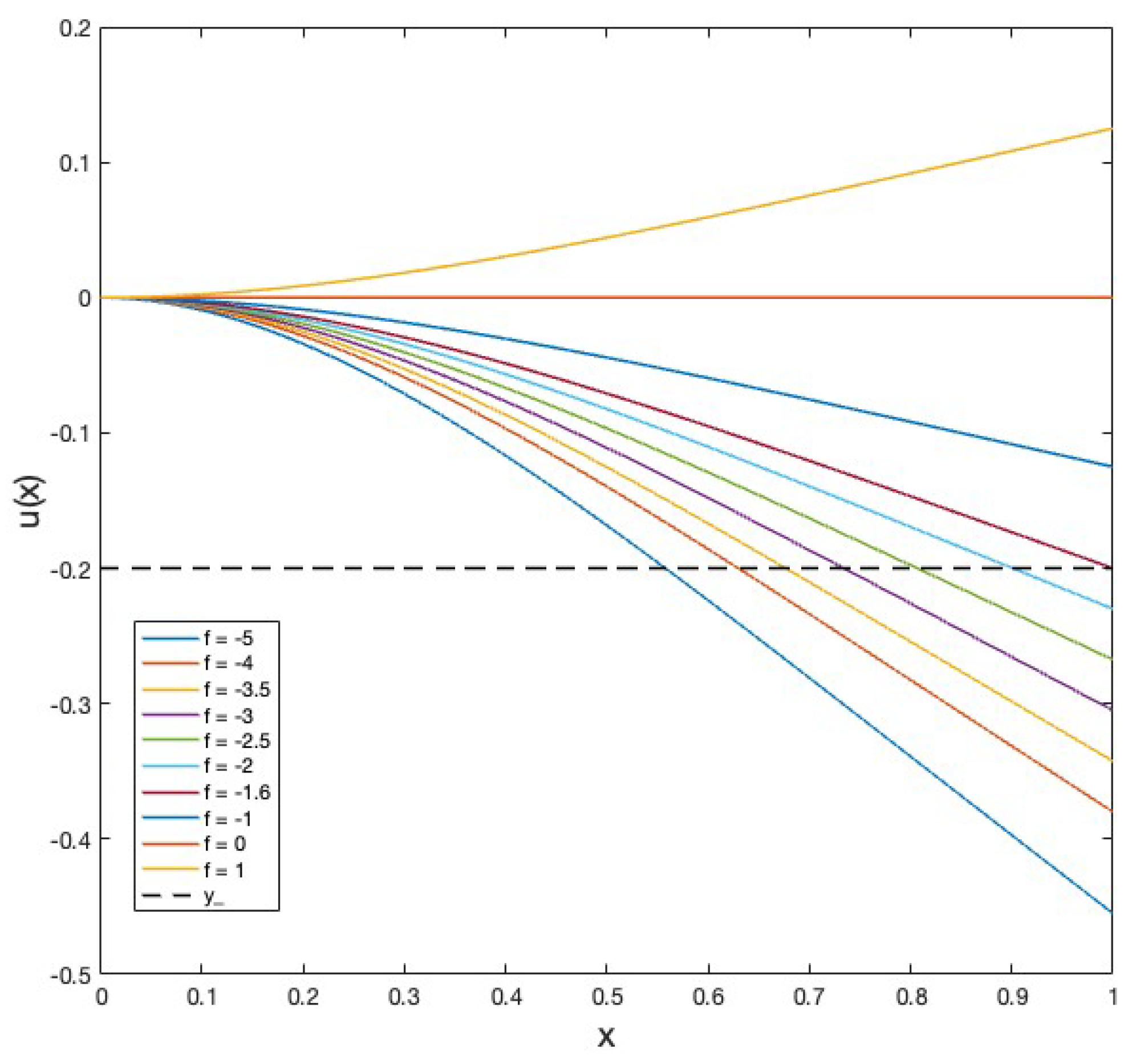
Figure 3.
Position of the right end of the beam over time for different values of and . The dashed black line represents the location of the obstacle. The red line corresponds to , the blue line to , green is and yellow is . Progressively the penetration decreases, and substantially changes between the values of and .
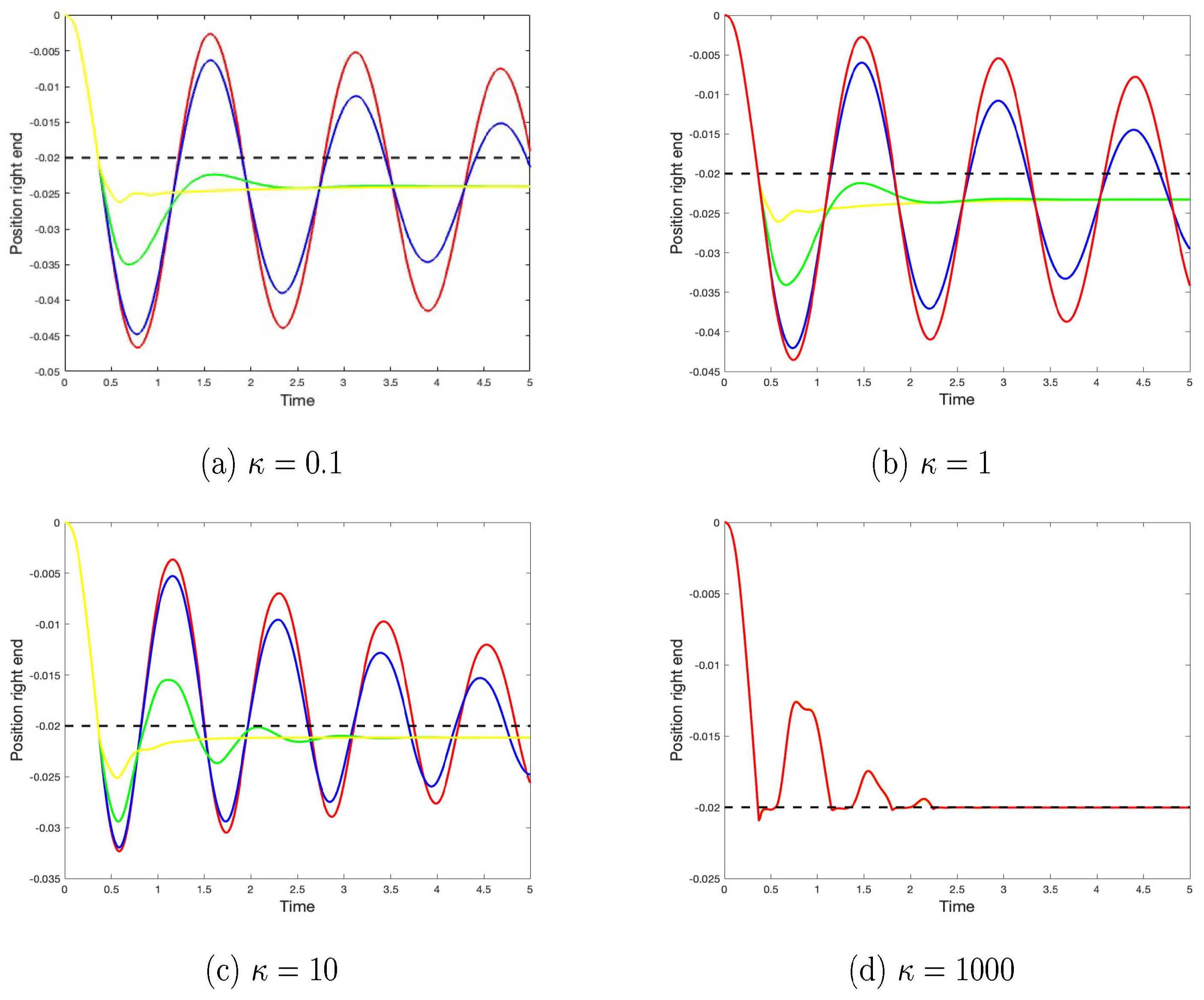
Figure 5.
log-log plot of and norms
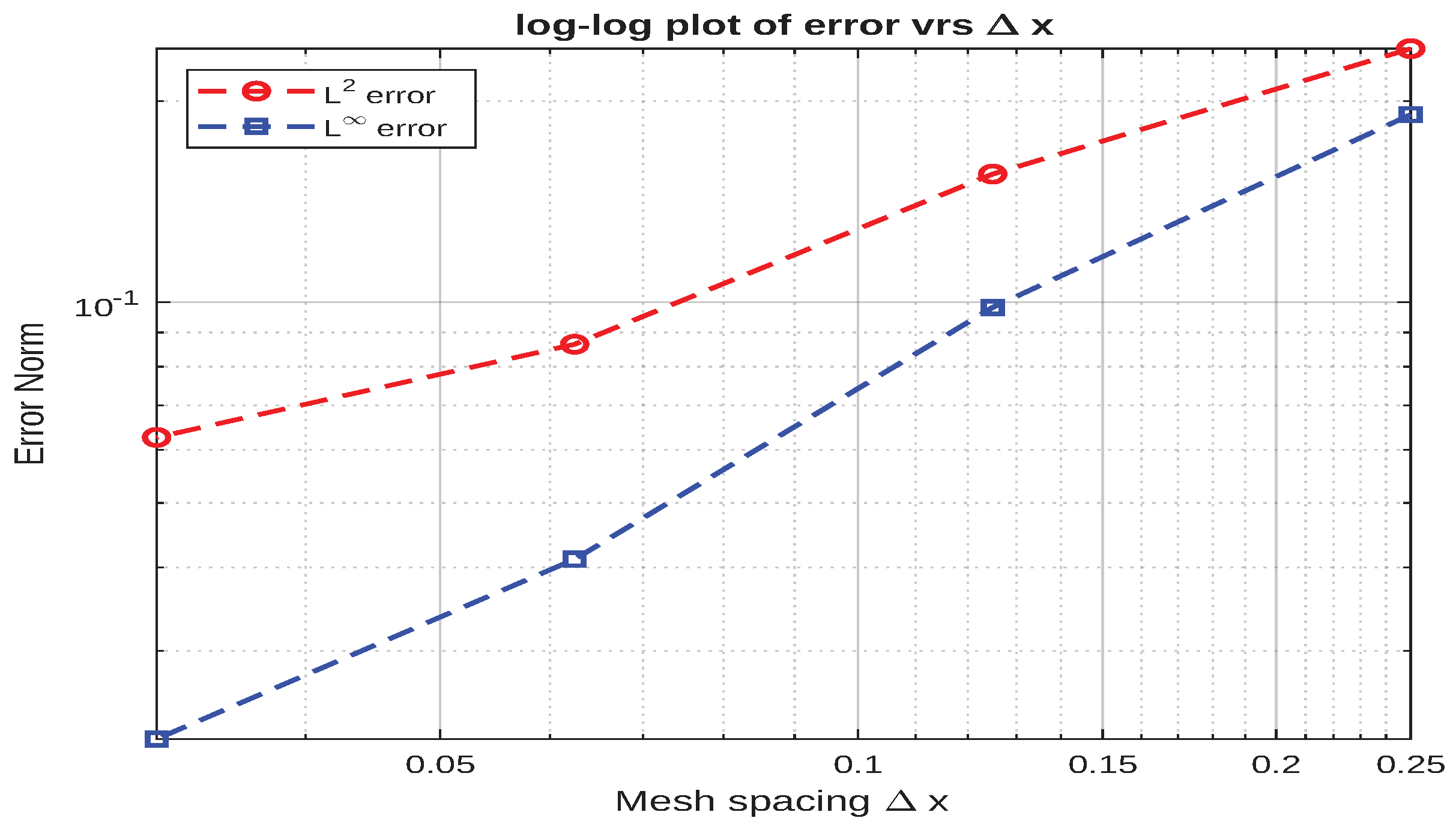

Table 1.
Comparing the numerical solution to the exact solution
| M | dx | L2 error | L∞ error |
|---|---|---|---|
| 4 | 0.25000 | 2.39706e-01 | 1.90937e-01 |
| 8 | 0.12500 | 1.55504e-01 | 9.81641e-02 |
| 16 | 0.06250 | 8.64282e-02 | 4.11572e-02 |
| 32 | 0.03125 | 6.26681e-02 | 2.21307e-02 |
Disclaimer/Publisher’s Note: The statements, opinions and data contained in all publications are solely those of the individual author(s) and contributor(s) and not of MDPI and/or the editor(s). MDPI and/or the editor(s) disclaim responsibility for any injury to people or property resulting from any ideas, methods, instructions or products referred to in the content. |
© 2025 by the authors. Licensee MDPI, Basel, Switzerland. This article is an open access article distributed under the terms and conditions of the Creative Commons Attribution (CC BY) license (http://creativecommons.org/licenses/by/4.0/).
Copyright: This open access article is published under a Creative Commons CC BY 4.0 license, which permit the free download, distribution, and reuse, provided that the author and preprint are cited in any reuse.


