
Submitted:
24 September 2025
Posted:
25 September 2025
You are already at the latest version
Abstract
When analysing digital images in metric spaces, several parameters based on image content and/or image structure can be used. Among these, a parameter that can be easily measured in practice for measuring self-similar images/image details is the fractal dimension or the fractal dimension-based quantities derived from it. All this makes it possible to perform measurements on individual or mass images or image details. However, the interpretation of the data obtained in this way raises several problems. The aim of this work is to describe the mathematical foundations of fractal dimension measurement characteristic of spectral content in digital images, by presenting it through practical examples. We also describe a possible solution regarding how the application of spectral image structure in practice can improve the interpretation and reliability of the measured results of box counting algorithms. We also examine the mathematical possibility of how the concept of spectral self-similar image structure and the entropy of the Second Law of Thermodynamics can help in the interpretation of image data obtained during living or inanimate natural science processes. By re-examining previous results and using new measurement results, we illustrate the role of geometry resolution in spectral fractal structure-based studies. Considering the entire Universe as a single sensor, we provide the main parameters of this sensor, including values characteristic of its spectral fractal structure.
Keywords:
fractal
; fractal structure
; Hausdorff Besicovitch dimension
; spectral fractal dimension
; entropy
; metric space
1. Introduction
One of the defining digital information media elements of our time is visual information. Within the animal kingdom, it is vital for mammals to perceive events in their environment based on visual data, to process them quickly and reliably, and to make decisions based on the information obtained. The medium of information transmission is most often electromagnetic waves. For terrestrial vegetation, the utilization of energy coming from the sun in the form of electromagnetic waves is vital not only for their own existence, but also for all life on earth. For humanity, visual data is perhaps one of the most important and effective information elements among the types of information necessary for development, which has been present for more than 51,000 years [1]. Nowadays, the perception of visual data in digital form and its digital processing with efficient - man-made - tools is of paramount importance.
Mandelbrot defined the concept of fractal as follows [2]: " A fractal is by definition a set for which the Hausdorff-Besicovitch dimension strictly exceeds the topological dimension". In practice, the above definition can be applied to digitally recorded data (e.g. images, sounds, videos) with a good approximation. However, in the case of complex image-data structures defined in different metric spaces and with different content, their measurement is difficult.
The Hausdorff–Besicovitch dimension was first introduced by Felix Hausdorff in 1918 and later developed by Abram S. Besicovitch. It can be defined for any subset of the real set as follows [3-4]:
Let C⊆ℝand given s≥0.
Then, the s-dimensional Hausdorff measure of C is:
and the Hausdorff dimension of C can be defined as follows:
𝐻(𝐶) = inf { 𝑠 ≥ 0 | 𝐻𝑠(𝐶) = 0 }.
The quantity H(C) is the Hausdorff–Besicovitch dimension of C. In most cases, H(C) is quite difficult to calculate. While the upper bound is relatively easy to determine, the lower bound is much more difficult to determine. Due to the inf in its definition, the Hausdorff–Besicovitch dimension cannot be measured for any physical object. We get closer to a practical definition by describing the fractal dimension theoretically [5].
Let be a metric space, and . Let N(ε) be the minimum number of spheres of radius ε that cover the set A.
If
exists, then FD is called the fractal dimension of the set.
The general measurable definition of fractal dimension (FD) is as follows:
where L1 and L2 are the lengths measured on the (fractal) curve, and S1 and S2 are the dimensions of the (arbitrary) measure used (e.g., the geometric resolution in the case of digital images). The calculation of the fractal dimension is simple and can be performed based on several well-known algorithms [6], (Box Counting [7], Epsilon-Blanket [8], Fractional Brownian Motion [9], Power Spectrum [9], Hybrid Methods [10], Perimeter–Area relationship [11], Prism Counting [12], Walking-Divider [13]). However, the practical application of these numerical methods was well outlined even in the early period [14,15].
The fundamental problem when using the fractal dimension defined by equation (4) is that it is insensitive to the shades and colours of the image. This is well illustrated in Figure 1, where we can see black and white, grayscale and 3 × 8-bit colour (RGB) images. Applying equation (4) with the box method, the measured FD values are the same in all three images (FD = 2). The solution to this problem can be the introduction of SFD [16] and its application during the measurements.

Table 1.
The values measured based on (5) and (9) of the images shown in Figure 1.
Table 1.
The values measured based on (5) and (9) of the images shown in Figure 1.
| Image type | Colour space /bit/ |
FD | SFDDSR /16bit/ |
EW-SFDDSR /real bit/ |
SFDDSR /real bit/ |
|---|---|---|---|---|---|
| Black-White | 1 | 2 | 0,2113 | 0,9332 | 1,0000 |
| Greyscale | 8 | 2 | 0,8312 | 0,9908 | 0,9999 |
| Palette | 8 | 2 | 0,8314 | 0,9659 | 1,0000 |
| RGB colour | 24 | 2 | 2,3513 | 2,7652 | 2,8869 |
Digital images taken with modern imaging devices today contain information from global navigation satellite systems (GNSS) and other location information systems and services within the EXIF data [17]. Based on these, images can be created that already contain height data for each pixel in the image. While orthophotos can also contain spectral data in addition to height data. The FD defined by (4) is suitable for measuring height data, but not for measuring spectral data (Figure 1).
To measure the spectral structure, the spectral fractal dimension (SFD), defined in [6,16], equation (5) can be used:
where
n – number of image layers or bands;
S – spectral resolution of the layer, in bits;
BMj – number of spectral boxes containing valuable pixels for j-bit;
BTj – total number of possible spectral boxes for j-bits.
The number of possible spectral boxes (BTj) for j-bits is as follows:
The metric (5) is therefore suitable for measuring self-similar structure in images [16]. Using equations (5) and (6), a generally measurable definition of the spectral fractal dimension is as follows, if the spectral resolution is the same within each image band (SFDEqual Spectral Resolution – SFDESR) (7):
If the spectral resolution is different per band/layer, then the generally measurable definition of the spectral fractal dimension (SFDDifferent Spectral Resolution – SFDDSR) is as follows [16]:
where
Si— spectral resolution of layer i, in bits.
As another possibility, we mention the relation presented in [18], which is the weighting of the self-similar spectral image structure with Shannon entropy [19,20], as follows:
The implementation of EW-SFD was developed to apply energetic, physical and biological laws together to separate useful information from highly noisy images.
The relations (5), (7), (8) and (9) are metrics, since in the case of metrics all of the following conditions must be fulfilled [16,21]:
- Non-negative definite, that is
- 2.
- Symmetrical, that is
- 3.
- It satisfies the triangle inequality, that is,
- 4.
- Regularity, this means that the points of the discrete image plane must be uniformly dense, i.e.
where A is an arbitrary subset of the N-dimensional image, while P is an arbitrary pixel of the N-dimensional image, and in the context of (13) above, SFD means the metrics according to (5), (7)–(9).
The Shannon entropy [19,20], which is interpreted as the weight factor of the independent pixels in the denominator of equation (9), is positive and finite. It cannot be zero, since in the case of metric spaces the zero-set (empty) image is not part of the space. The finite condition is also satisfied because in practice every digital image consists of a finite number of pixels, so the spectral space also has a finite number of elements. Based on the above, the previously presented proof (SFD as a metric) is also valid for equations (7–9) [21].
In [21], the following relationship was introduced for the SFD-based characterization of some technical parameters of image sensors in a single parameter (Spatial and Spectral Resolution Range - SSRR):
where
K – the number of pixels that make up the image.
The value of this quantity increases monotonically if any two of the values of S, n and K given in (5) are fixed and the third value increases. (14) contains all three characteristic parameters, so it can be a characteristic value for any digital image sensor.
The distribution of the dimensions defined in equations (5), (7-9) with respect to height, time or temperature, which, under given boundary conditions, can be interpreted for a given natural or artificial object, can be considered as the spectral height, time or temperature fingerprint of the given object, as follows [22]:
where
- n—number of image (h, t, T) excluding layers or bands;
- S—spectral resolution of the (h, t, T) excluding layer, in bits;
- BMj (h, t, T)—number of spectral boxes containing valuable pixels in case of j-bits (h, t, T) distributions;
- BTj (h, t, T)—total number of possible spectral boxes in case of j-bits (h, t, T) distributions.
Below are the values of n used in practice.
- n=1 black and white or greyscale image
- n=2 joint measurement of two bands used for index analysis (e.g. NDVI, SAVI based indices)
- n=3 RGB, YCC, HSB, IHS colour space image
- n=4 traditional colour printer CMYK space image, some CMOS sensor or Landsat 1–5 Multispectral Scanner (MSS)
- n=6 photo printer CCpMMpYK space image, Landsat ETM satellite images
- n=7 Landsat 4–5 Thematic Mapper (TM)
- n=8 Landsat 7 Enhanced Thematic Mapper Plus (ETM+)
- n=10 MicaSense Dual Camera System (Red and Blue)
- n=11 Landsat Operational Land Imager (OLI) for optical bands and the Thermal Infrared Sensor (TIRS) for thermal bands
- n=13 Sentinel-2A satellite sensor
- n=30 CHNSPEC FS-50/30
- n=32 DAIS7915 VIS-NIR or DAIS7915 SWIP-2 sensors
- n=60 COIS VNIR sensor
- n=79 DAIS7915 all
- n=126 HyMap sensor
- n>250 CHNSPEC FigSpec Series Full-Spectrum Hyperspectral Imager FS-2A
- n=254 AISA Hawk sensor
- n=488 AISA Eagle sensor
- n=498 AISA Dual sensor (Eagle and Hawk)
The fractal concept formulated by Mandelbrot and the significance of the related dimension were first widely presented in [23] in 1967. The practical extension of the concept of fractal dimension (FD) was further developed with the emergence of multifractals, with the presentation of the possibilities of application within physics [24] in 1983. A significant milestone is the summary textbook published in 2020, the main topic of which is the presentation of the possibilities of application of fractal dimension in network systems, but with regard to dimension it also contains a broad outlook on applications in other fields [25].
The spectral fractal dimension-based relationships have been and are still being applied in many areas. The introduction of spectral fractal structure and spectral fractal dimension in image processing took place in the framework of conference presentations in 2004 [26,27]. The presentation of initial applications [6,26,27,28] pointed to a wide range of possibilities. Such was the separation of cane fungus pathogenic species by measuring the geometric changes on the surface of cane leaves and the spectral structure of the changes in 8-bit image bands. SFD has also been successfully used to measure the colour resolution of 3D models made from geocoded aerial photographs [28,29]. The examination of the spectral and geometric patterns of sawn wood boards was mentioned as an additional possibility [6,29]. The presented results clearly demonstrated that the spectral fractal dimension can be effectively applied even in the case of 8-bit RGB images per band. Further possibilities were presented for seed separation, dose effects on herbicide-treated sweet corn images, and leaf damage studies. In a controlled, laboratory-based psychovisual study of the JPEG compression process for measuring certain spectral characteristics, the SFD according to (5) was used to select test images [30,31]. The classification of potato tubers and the successful measurement of their quality characteristics based on SFD clearly highlighted the importance of the hue resolution of the images included in the study, both for RGB and FIR images [32]. Here and in [33], the study of temporal damage to plant parts was mentioned and applied. The researchers also drew attention to the importance of local measurements on samples.
In 2007, SFD measurements were performed according to (5) presented in [34] for the analysis of hyperspectral images taken by the DAIS 7915 sensor. SFD values were measured for different vegetation types (alfalfa, sugar beet, corn, winter wheat, weeds, and turf), channel by channel and for all 80 channels. The aim was to separate the individual plant species using spectral curves prepared based on SFD values. The effect of noisy channels on the runtime was also presented in the same work. The basics of classifying hyperspectral images based on SFD spectral curves were presented in [35]. During the classification, four different crops (corn, triticosecale, wheat, sunflower), fallow land, trees and dirt roads were separated based on AISA DUAL hyperspectral images by analysing SFD spectral curves - as a kind of fingerprint. It has been found that noise in the entire image degrades the colour structure, i.e. SFD values decrease significantly and rapidly, or even oscillate. Using the relationships proposed by Clevers et al., [36] and Mutanga and Skidmore [37], the red edge inflection point location (REIP-SFD) in nanometres, which can be determined from the SFD curves, was defined as follows [35]:
λre = 690 + 30 {SFDAVERAGE (690-720)}
During the aerial survey of the red mud disaster [38,39,40], the metric (5) was used to locally identify flow areas and distinguish flow types, while processing images in the visible (VIS), near-infrared (NIR) and far-infrared (FIR) spectral ranges [41]. They concluded that stationary, laminar, and turbulent tracks can be examined not only by geometric analysis of the flow area pattern in the aerial photograph of the remaining mud. The flow types can be distinguished by measuring (5) and by examining the fractal structure in spectral space of hyperspectral or multispectral aerial photographs.
In the impact assessment of traffic-related pollutants, SFD and Shannon entropy were compared. Based on images taken in the second half of the growing season, it can be clearly stated that in the case of maize, the average information content (entropy) gives the highest value in images taken in the near-infrared range. However, the entropy-based analysis did not show differences between the individual treatments in any spectral range. However, the analysis based on spectral fractal structure (5) to detect these showed significant differences [42,43].
A fractal dimension calculation method called compression fractal dimension has also been published, which can determine the fractal dimension estimate in an image-independent manner [44]. The noise dependence of the generated fractal dimension was investigated on scanned digital images using three well-known algorithms (Pair-Counting Correlation, Box-Counting, Fixed-Grid Correlation) in the work [45]. Out of the seven conclusions, three important elements would be highlighted: 1. the presence of noise in digital images strongly influences the algorithms generally used for calculating the fractal dimension, 2. pixel-based methods are generally more robust to noise, and 3. the box-counting approach is not reliable enough. All three conclusions are confirmed by the author, however, to improve the reliability of the third statement, this work will propose a possible solution in the future, which is an estimation algorithm-independent solution. Several other works have also been published, which propose the refinement of fractal dimension calculation algorithms on digital images - in a targeted manner. Such methods include dimension estimation based on multiple geometric features [46] and the image pyramid approach [47].
The possibility of examining the spectral fractal structure is also mentioned in many other areas. Such as the classification of Earth observation satellite systems based on a uniform scale [48], the prognosis of multiple sclerosis [49] and the analysis of CT images [50]. It was used to check the reliability of measurement data in the work [51], where the quality of certain wheat varieties was estimated using image processing methods based on laboratory measurements. During the investigation of imaging algorithms based on RAW images taken by Bayer-based image sensors, equation (7) was used to select test images in the work [52]. In the publication [53], the measurement of the gain noise of Bayer-type image sensors based on parameters that can be decisive for higher-level processing processes (segmentation, classification, recognition) is presented. Equations (7) and (8) have been successfully applied to measure the gain noise of different image sensors used in the vision systems of different types of drones, as well as to some elements of optimal data acquisition and processing. It was also used to analyse the data depth and structure of test images [54] when examining the impact of individual imaging algorithms on image classification procedures (Mahalonobis Distance, Maximum Likelihood, Minimum Distance, Parallelepiped, Spectral Angle Mapper and Spectral Information Divergence). The first experimental verification of the ultraweak photon emission of mouse embryos played a key role in the joint application of medicine, biology, physics, and computer science, EW-SFD according to (9) [18,55]. Based on equation (9), it became possible to detect a significant difference between live, degenerate and background samples in digital images with an extremely low signal-to-noise ratio. The relationships (7-9) were used in the selection of images included in the studies in structured similarity index (SSIM)-based analysis [56], in vegetation mapping [57], and in the comparative analysis of NDVI indices calculated from multitemporal and Bayer-type RGB images [58].
The fractal structure-based analysis of digital images offers several additional possibilities. If we want to supplement the image and other data related to the image (e.g. ground references) with structural data that can be measured in metric spaces, then one of the most frequently measured parameters can be the fractal dimension according to (7-9). In such cases, it is advisable to consider the concept of density used in the mathematical sense.
When the topology X is given by a metric, the closure of A in X is the union of A and the set of all limits of sequences of elements in A (its limit pixels) [2,21,59,60,61],
Then, A is dense in X if
Equations (17) and (18) are approximately fulfilled in practice for digital images and imply several conditions for image sensor chips, pixel readout and image file formats [22]. In the case of image sensor chips, the condition primarily means the same geometric size of the pixel sensor elements in the x, y directions and the same cell size within the entire chip. This is usually fulfilled in industrial devices for space, aircraft, and UAV image sensors. During readout, omitting data from several pixel rows/columns at the edges of the sensors in the final image significantly improves the signal-to-noise ratio of the pixels at the edges. However, optical distortions and inadequate geometric mapping deteriorate the signal-to-noise ratio. In the case of professional UAV camera systems, the distortion caused by mapping can be significantly improved with an appropriate optical system. In the case of the file format, the condition is the accurate storage of the image sensor chip data (in the form of metadata within the images) in a lossless, raw image format, based on standards. However, it is advisable to check the fulfilment of the conditions outlined above based on the technical data of the UAV devices.
2. Materials and Methods
The algorithms used to determine the fractal dimension of digital images [7, 62] are applied down to the finest geometric detail. This means that the iteration procedure can be applied starting from the entire image down to the size of a single pixel. If we move to the space containing spectral values, instead of the geometric resolution, the intensity values of the individual layers/bands in independent directions are used (Figure 2). Therefore, in practice, we can determine the iteration steps based on the intensity values.
The intensity values of digital images detected with sensors are determined - based on the above - by the intensity values of the sensors. If these image data are modified/processed by software before the measurements (e.g. noise filtering, modification for image display, classification, etc.), then the modification is also an interesting aspect. The last, but also essential element is the characteristics of the file format of the saved image data.
Considering the aspects described above, the author proposes and applies several calculation options during SFD-based measurements:
- A.
- 8 bit – SFDESR, SFDDSR and EW-SFD
- A.
- B. 16 bit - SFDESR, SFDDSR and EW-SFD
- A.
- C. real bit - SFDESR, SFDDSR and EW-SFD
In case “A”, the spectral data in the first 8 bits per band is measured regardless of the actual content. In the case of purely 8-bit image data or format types, this can be applied in the same way as in case “C”.
In case “B”, the spectral data in the first 16 bits per band is measured regardless of the actual content. In the case of purely 16-bit image data or format types, this can be applied in the same way as in case “C”.
While in case “C”, real spectral data is measured regardless of the representation or format occurring in each band.
3. Results
3.1. Measuring Image Data of Camera Arrays
Figure 3 shows the image data of the sensor in four independent spectral ranges, but placed in a single camera array, as shown in Figure 2 of [22].
Table 2.
The images shown in Figure 3 are the measured values of all possible channel variations, based on (9).
Table 2.
The images shown in Figure 3 are the measured values of all possible channel variations, based on (9).
| Image band(s) | EW-SFD /8 bit/ |
EW-SFD /16 bit/ |
EW-SFDDSR /real bit/ |
|---|---|---|---|
| R | 0,2117 | 0,5886 | 0,5886 |
| G | 0,1358 | 0,5501 | 0,5501 |
| RE | -0,0879 | 0,4093 | 0,4093 |
| NIR | -0,5485 | 0,1702 | 0,1702 |
| Average of previous four values | -0,0722 | 0,4295 | 0,4295 |
| R and G | 0,8034 | 1,2018 | 1,1861 |
| R and RE | 0,7999 | 1,2085 | 1,2085 |
| R and NIR | 0,7622 | 1,1928 | 1,1756 |
| G and RE | 0,8841 | 1,2605 | 1,2476 |
| G and NIR | 0,7388 | 1,1829 | 1,1651 |
| RE and NIR | 0,3999 | 0,9898 | 0,9598 |
| Average of previous six values | 0,7314 | 1,1727 | 1,1571 |
| R-G-RE | 1,3296 | 1,5885 | 1,5985 |
| R-G-NIR | 1,2665 | 1,5584 | 1,5664 |
| G-RE-NIR | 1,2422 | 1,5486 | 1,5560 |
| R-RE-NIR | 1,2099 | 1,5301 | 1,5362 |
| Average of previous four values | 1,2620 | 1,5564 | 1,5643 |
| R-G-RE-NIR | 1,6531 | 1,7738 | 1,7979 |
Based on the comparison of the data, increasing the number of bands (1,2,3 or 4) shows a clear increase in EW-SFD. This is also clearly illustrated in the diagram made from the data (Figure 4).
In our opinion, fractal dimension measurements and analyses performed together on 8, 16 and real bits can improve the reliability of box counting algorithms.
3.2. Spectral Analysis of RGB Images of Potato Tubers
We performed the measurements according to (9) in addition to (5) on the complete database images containing different potato tubers described in [32,33] (Figure 5). By using (5) and (9) together (with the appropriate weighting of the two parameters), all 14 potato tuber varieties became significantly separable, while previously according to (5) the authors could only give a significant separation of 4 potato tuber varieties. By measuring the tubers within each variety independently and then calculating the average, we obtain the following results in the case of White Lady: SFDDSR=2,0186±0,0262 és EW-SFDDSR=1,6716±0,0419. The differences are primarily due to the lower geometric resolution of the individual tuber images. In the case of lower geometric resolution, the number of points with different colors is determined by the geometric resolution.
Table 3.
The values measured based on (5) and (9) in the images shown in Figure 5.
Table 3.
The values measured based on (5) and (9) in the images shown in Figure 5.
| Potato variety | EW-SFDDSR /real bit/ |
SFDDSR /real bit/ |
Average |
|---|---|---|---|
| Réka | 2,0240 | 2,3187 | 2,17135 |
| rebeka | 2,0626 | 2,3403 | 2,20145 |
| Agata | 2,0391 | 2,3246 | 2,18185 |
| Arosa | 1,9885 | 2,3290 | 2,15875 |
| Ronina | 2,0464 | 2,3283 | 2,18735 |
| Impala | 1,7476 | 2,1957 | 1,97165 |
| Rosita | 1,6624 | 2,1710 | 1,9167 |
| amorosa | 2,1406 | 2,4204 | 2,2805 |
| Derby | 2,0990 | 2,3648 | 2,2319 |
| white lady | 1,9425 | 2,2455 | 2,094 |
| Roko | 1,9396 | 2,2634 | 2,1015 |
| Aladin | 1,9723 | 2,2943 | 2,1333 |
3.3. Standard-Model Based Image Sensor
Finally, we estimate the entropy and SFD values for the entire Universe, if the entire Universe behaves as a single sensor (Standard-model based Image Sensor - SmIS). Let us consider our sensor in such a way that each elementary particle of material nature forms an elementary point of the sensor (SmIS pixel). Let us examine the elementary particles of our material world based on Figure 6. Each sensing point can be described by three independent characteristics: Mass, Charge and Spin. Following the RGB analogy, we will refer to this as MCS in the future. Let us see – based on Figure 6 – how many different values are found in each independent MCS space, and then how many bits can we describe these values in. The above is summarized in Table 4. According to the table, there are 16 different masses (described in 4 bits), 5 types of charges (described in 3 bits) and 3 types of spin (described in 2 bits). All this can be described in MCS space in a total of 9 bits (4 bits, 3 bits, 2 bits), i.e. each SmIS pixel in MCS space can be characterized by a triplet of numbers. If we also take antimatter into account, the above changes as follows: 16 different masses (can be described in 4 bits), 7 types of charges (can be described in 3 bits) and 5 types of spins (can be described in 3 bits), i.e. we need 10 bits.
To calculate the SFD, we need the number of elementary particles in the Universe, since they constitute the number of image sensors of our SmIS sensor. Based on the work [63], this number is approximately 1080. Based on all this, the size of the entire image is: 2x1080 bytes.
Based on the equation (6), it can be given how many optimal images (n) we would need to place a valuable SmIS pixel in each box, i.e., to maximize our SFD value. In our case, this is 267, i.e., all this is achievable with a 267-channel optimal SmIS image. Assuming multitemporal data collection, this means that we need to take images at least 89 (267/3) different times. In practice, images taken are not optimal, so recording at significantly more times would be necessary.
If we accept that the shortest unit of time for the change in the information content of the Universe is the Planck time (this is the time it takes a photon in a vacuum to travel a distance of one Planck length at the speed of light), tP~5,39x10-44 s), we can determine how many SmIS recordings could have been made during the known age of the Universe (tU~4,36x10¹⁷ s). In our case, this is the image number: 8,08x1060.
Based on equation (14), the SSRR value can also be given to our SmIS sensor, which can take the following values: SSRRmass = 24, SSRRmass-antimatter = 27
4. Discussion
When analysing digital images in metric spaces, a parameter that can be easily measured in practice for measuring self-similar images/image details is the fractal dimension or the entropy-weighted fractal dimension. This makes it possible to measure individual or mass images or image details. However, the interpretation of the data obtained in this way raises several problems. This work summarizes the mathematical foundations of the fractal dimension measurement characteristic of the spectral content in digital images. It discusses their metric properties (non-negative definiteness, symmetry, triangular inequality and regularization). It discusses the weighting of the spectral fractal dimension with Shannon entropy. It presents the Spatial and Spectral Resolution Range relation proposed for the uniform parameterization of image sensors.
The possibility of SFD and EW-SFD is presented through practical examples. The work highlights how the application of spectral image structure in practice can improve the interpretation of the measured results of box counting algorithms and their reliability. It is proposed that fractal dimension measurements and analyses be performed simultaneously on 8, 16 and real bits. Although SFD-based measurements were presented separately in previous works, none of them dealt with the joint interpretation of these data.
The author considers one of his most significant results to be that in the case of noisy images, the measurement of useful information related to either the noise or the signal provides reliable results without modifying the original images. Details of this were presented in [18]. In this work, the weighting of the spectral self-similar image structure with Shannon entropy was introduced and applied as a measured parameter. At the same time, the concept of entropy of the second law of thermodynamics helped the physical interpretation of the entire biological process, both for living and non-living (including the image sensor) objects. This is also one of the most important findings of the present work.
Through the spectral fractal structure-based measurement of potato tubers, it was demonstrated to what extent the related newer SFD-based metric parameters can improve the results of previous measurements.
Finally, the author, through the introduction and example of the Standard-model based Image Sensor, considers it justified and recommends SFD and EW-SFD-based measurements on original images occurring in astronomy. This can also be considered a possible future challenge.
5. Conclusions
The spectral fractal structure (SFD)-based measurement of digital images provides numerical data for the analysis of the self-similar image structure of a complex, multi-channel image data. In addition to camera arrays or multi-channel sensor systems, the method can also be used for other image multi-dimensional data structures (MRI, CT, PET, orthophotos). The fractal dimension measurements and analyses performed together at 8, 16 and real bits can improve the reliability of box counting algorithms and the conclusions drawn. The measurement data of the spectral fractal structure weighting with information theoretical entropy, supplemented by the appropriate interpretation of the physical entropy concept in a given natural process, can open new possibilities in the measurement and interpretation of the self-similar structural characteristics of complex processes.
Funding
Project no. TKP2021-NVA-05 has been implemented with the support provided by the Ministry of Innovation and Technology of Hungary from the National Research, Development and Innovation Fund, financed under the TKP 2021 funding scheme.
Data Availability Statement
The original contributions presented in this study are included in the article; further inquiries can be directed to the author.
Acknowledgments
The author would like to thank the researchers at the Department of Drone Technology and Image Processing, Dennis Gabor University, for their useful advice and suggestions that significantly helped in the preparation of this study. I would like to thank my daughter and her lovely partner for their advice and corrections during the creation of the images and illustrations in this work. I am grateful to Hévíz-Balaton Airport for its air control during the execution of the operation and for its meteorological support for the practical implementation. I am especially grateful to the staff of the Balaton Upland National Park, the West Transdanubian Water Management Directorate, and the Kis-Balaton Engineering District for their helpful and useful advice.
Conflicts of Interest
The authors declare no conflicts of interest.
Abbreviations
| AISA Dual | Specim AISA Dual Hyperspectral sensor |
| AISA Eagle | Specim Eagle Hyperspectral sensor |
| AISA Hawk | Specim Hawk Hyperspectral sensor |
| BMj | number of spectral boxes containing valuable pixels for j-bit |
| BTj | total number of possible spectral boxes for j-bits |
| BW | Black and White (1 bit) |
| AVIRIS | NASA Airborne visible/infrared imaging spectrometer |
| NIR | Near-InfraRed |
| CT | Computer Tomography |
| DAIS | Digital Airborne Imaging Spectrometer |
| DEM | Digital Elevation Model |
| E | Entropy |
| ETM+ | Landsat 7 Enhanced Thematic Mapper Plus |
| H(C) | Hausdorff–Besicovitch Dimension |
| MS | Multispectral |
| EW-SFD | Entropy-Weighted Spectral Fractal Dimension |
| FD | Fractal Dimension |
| FIR | Fared InfraRed |
| GND | Ground (altitude relative to take-off point) |
| MCS | Mass, Charge, Spin (analogue as RGB color-space) |
| MS-NIR | Multispectral camera array Near-InfraRed band |
| MS-R | Multispectral camera array R band |
| MS-RE | Multispectral camera array Red-Edge band |
| MSS | Landsat 1-5 Multispectral Scanner |
| MS-G | Multispectral camera array G band |
| NIR | Near Infrared |
| OLI | Landsat 8-9 Operational Land Imager optical bands |
| RE | Red-Edge |
| REIP-SFD | Red Edge Inflection Point on SFD curves |
| RGB | Red, Green, Blue (as color-space) |
| RGB-B | B band of RGB image of Bayer sensor |
| RGB-G | G band of RGB image of Bayer sensor |
| RGB-R | R band of RGB image of Bayer sensor |
| S | spectral resolution of the layer, in bits |
| SFD | Spectral Fractal Dimension |
| SmIS | Standard-model based Image Sensor |
| TIRS | Landsat 8-9 Thermal Infrared Sensor |
| TM | Landsat 4–5 Thematic Mapper Satellite |
| tP | Planck time |
| tU | Age of the Universe |
| UAV | Unmanned Aerial Vehicle |
| UAS | Unmanned Aerial System |
| VIS | Visible |
References
- Oktaviana, A.A. , Joannes-Boyau, R., Hakim, B. et al. Narrative cave art in Indonesia by 51,200 years ago. Nature 2024, 631, 814–818. [Google Scholar] [CrossRef]
- Mandelbrot, B.B. The Fractal Geometry of Nature; W.H. Freeman and Company: New York, NY, USA, 1983; p. 15. [Google Scholar]
- Soltanifar, M. A Generalization of the Hausdorff Dimension Theorem for Deterministic Fractals. Mathematics 2021, 9, 1546. [Google Scholar] [CrossRef]
- Falconer, K. Fractal Geometry: Mathematical Foundations and Applications, 3rd ed.; John Wiley & Sons: Chichester, UK, 2014; p. 44, 45, 48, 49, 72, 112. [Google Scholar]
- Barnsley, M.F. Fractals Everywhere; Academic Press: Cambridge, MA, USA, 1998; pp. 182–183. [Google Scholar]
- Berke, J. Spectral fractal dimension. In Proceedings of the 7th WSEAS Telecommunications and Informatics (TELE-INFO ’05), Prague, Czech Republic, 12–14 March 2005; pp. 23–26. [Google Scholar]
- Voss, R. Random fractals: Characterisation and measurement. In Scaling Phenomena in Disordered Systems; Pynn, R., Skjeltorps, A., Eds.; Plenum: New York, NY, USA, 1985. [Google Scholar]
- Peleg, S.; Naor, J.; Hartley, R.; Avnir, D. Multiple Resolution Texture Analysis and Classification. IEEE Trans. Pattern Anal. Mach. Intell. 1984, 4, 518–523. [Google Scholar] [CrossRef] [PubMed]
- Turner, M.T.; Blackledge, J.M.; Andrews, P.R. Fractal Geometry in Digital Imaging; Academic Press: Cambridge, MA, USA, 1998; p. 45–46, 113-119. [Google Scholar]
- Goodchild, M. Fractals and the accuracy of geographical measure. Math. Geol. 1980, 12, 85–98. [Google Scholar] [CrossRef]
- DeCola, L. Fractal analysis of a classified Landsat scene. Photogramm. Eng. Remote Sens. 1989, 55, 601–610. [Google Scholar]
- Clarke, K. Scale based simulation of topographic relief. Am. Cartogr. 1988, 12, 85–98. [Google Scholar] [CrossRef]
- Shelberg, M. The Development of a Curve and Surface Algorithm to Measure Fractal Dimension. Master’s Thesis, 1982, Ohio State University, Columbus, OH, USA.
- Barnsley, M.F.; Devaney, R.L.; Mandelbrot, B.B.; Peitgen, H.-O.; Saupe, D.; Voss, R.F.; Fisher, Y.; McGuire, M. The Science of Fractal Images; Springer: New York, NY, USA, 1988. [Google Scholar]
- Theiler, J. Estimating fractal dimension. J. Opt. Soc. Am. A 1990, 7, 1055–1073. [Google Scholar] [CrossRef]
- Berke, J. Measuring of spectral fractal dimension. New Math. Nat. Comput. 2007, 3, 409–418. [Google Scholar] [CrossRef]
- Standard of the Camera & Imaging Products Association; CIPA DC- 008-Translation-2024, 2024, pp. 76-86., https://www.cipa.jp/std/documents/download_e.html?CIPA_DC-008-2024-E.
- Berke, J.; Gulyás, I.; Bognár, Z.; Berke, D.; Enyedi, A.; Kozma-Bognár, V.; Mauchart, P.; Nagy, B.; Várnagy, Á.; Kovács, K.; et al. Unique algorithm for the evaluation of embryo photon emission and viability. Sci. Rep. 2024, 14, 15066. [Google Scholar] [CrossRef]
- Shannon, C.E. A mathematical theory of communication. Bell Syst. Tech. J. 1948, 27, 379–423. [Google Scholar] [CrossRef]
- Shannon, C.E. Prediction and entropy of printed English. Bell Syst. Tech. J. 1951, 30, 50–64. [Google Scholar] [CrossRef]
- Berke, J. Using spectral fractal dimension in image classification. In Innovations and Advances in Computer Sciences and Engineering; Sobh, T., Ed.; Springer: Berlin/Heidelberg, Germany, 2010; pp. 237–242. [Google Scholar]
- Berke, J. Application Possibilities of Orthophoto Data Based on Spectral Fractal Structure Containing Boundary Conditions. Remote Sens. 2025, 17, 1249. [Google Scholar] [CrossRef]
- Mandelbrot, B. How long is the coast of Britain? Statistical self-similarity and fractional dimension. Sci. New Ser. 1967, 156, 636–638. [Google Scholar]
- Hentschel, H.G.E.; Procaccia, I. The Infinite Number of Generalized Dimensions of Fractals and Strange Attractors. Phys. D 1983, 8, 435–444. [Google Scholar] [CrossRef]
- Rosenberg, E. Fractal Dimensions of Networks, Springer: Cham, Switzerland, 2020.
- Berke, J. Fractal dimension on image processing. In Proceedings of the 4th KEPAF Conference on Image Analysis and Pattern Recognition, Miskolc-Tapolca, Hungary, 28–30 January 2004; Volume 4, p. 20. [Google Scholar]
- Berke, J. The Structure of dimensions: A revolution of dimensions (classical and fractal) in education and science. In Proceedings of the 5th International Conference for History of Science in Science Education, Conference, Keszthely, 12–16 July 2004. [Google Scholar]
- Berke, J. Real 3D terrain simulation in agriculture. In Proceedings of the 1st Central European International Multimedia and Virtual Reality Conference, Veszprém, Hungary, 6–8 May 2004; Volume 1, pp. 195–201. [Google Scholar]
- Berke, J. Applied spectral fractal dimension. In Proceedings of the Joint Hungarian-Austrian Conference on Image Processing and Pattern Recognition, Veszprém, Hungary, 11–13 May 2005; pp. 163–170. [Google Scholar]
- Busznyák, J.; Berke, J. Psychovisual comparison of image compression methods under laboratory conditions. In Proceedings of the 4th KEPAF Conference on Image Analysis and Pattern Recognition, Miskolc-Tapolca, Hungary, 28–30 January 2004; Volume 4, pp. 21–28. [Google Scholar]
- Berke, J.; Busznyák, J. Psychovisual Comparison of Image Compressing Methods for Multifunctional Development under Laboratory Circumstances. WSEAS Trans. Commun. 2004, 3, 161–166. [Google Scholar]
- Berke, J.; Polgár, Z.; Horváth, Z.; Nagy, T. Developing on exact quality and classification system for plant improvement. J. Univers. Comput. Sci. 2006, 12, 1154–1164. [Google Scholar]
- Berke, J. Measuring of Spectral Fractal Dimension. In Proceedings of the International Conferences on Systems, Computing Sciences and Software Engineering, 10-20 December 2005; Paper No. 62., (SCSS 05).
- Kozma-Bognár, V. The application of Apple systems. J. Appl. Multimed. 2007, 2, 61–70. [Google Scholar]
- Kozma-Bognar, V.; Berke, J. New Evaluation Techniques of Hyperspectral Data. J. Syst. Cybern. Inform. 2009, 8, 49–53. [Google Scholar]
- Clevers, J.G.P.W.; De Jong, S.M.; Epema, G.F.; Van Der Meer, F.D.; Bakker, W.H.; Skidmore, A.K.; Scholte, K.H. Derivation of the red edge index using the MERIS standard band setting, International Journal of Remote Sensing, 2002, 23 (16), 3169–3184.
- Mutanga, O.; Skidmore, A. K. ; Integrating imaging spectroscopy and neural networks to map grass quality in the Kruger National Park, South Africa, Remote Sensing of Environment, 2004, 90. 104– 115.
- Berke, J.; Bíró, T.; Burai, P.; Kováts, L.D.; Kozma-Bognar, V.; Nagy, T.; Tomor, T.; Németh, T. Application of remote sensing in the red mud environmental disaster in Hungary. Carpathian J. Earth Environ. Sci. 2013, 8, 49–54. [Google Scholar]
- Bíró, T.; Tomor, T.; Lénárt, C.S.; Burai, P.; Berke, J. Application of remote sensing in the red sludge environmental disaster in Hungary. Acta Phytopathol. Entomol. Hung. 2012, 47, 223–231. [Google Scholar] [CrossRef]
- Burai, P.; Smailbegovic, A.; Lénárt, Cs.; Berke, J.; Milics, G.; Tomor, T.; Bíró, T. Preliminary Analysis of Red Mud Spill Based on Ariel Imagery. Acta Geogr. Debrecina Landsc. Environ. 2011, 5, 47–57. [Google Scholar]
- Berke, J.; Kozma-Bognár, V. Investigation possibilities of turbulent flows based on geometric and spectral structural properties of aerial images. In Proceedings of the 10th National Conference of the Hungarian Society of Image Processing and Pattern Recognition, Kecskemét, Hungary, 27–30 January 2015; pp. 295–304. [Google Scholar]
- Kozma-Bognár, V.; Berke, J. Entropy and fractal structure based analysis in impact assessment of black carbon pollutions. Georg. Agric. 2013, 17, 53–68. [Google Scholar]
- Kozma-Bognar, V.; Berke, J. Determination of optimal hyper- and multispectral image channels by spectral fractal structure. In Innovations and Advances in Computing, Informatics, Systems Sciences, Networking, and Engineering; Lecture Notes in Electrical Engineering, (LNEE), Sobh, T., Elleithy, K., Eds.; Springer International Publishing: Cham, Switzerland, 2015; Volume 313, p. 255–262. [Google Scholar]
- Chamorro-Posada, P. A simple method for estimating the fractal dimension from digital images: The compression dimension. Chaos Solitions Fractals 2016, 91, 562–572. [Google Scholar] [CrossRef]
- Reiss, M. A.; Sabathiel, N.; Ahammer, H. Noise dependency of algorithms for calculating fractal dimensions in digital images, Chaos, Solitons & Fractals, 2015, 78, 39-46.
- Spodarev, E.; Straka, P.; Winter, S. Estimation of fractal dimension and fractal curvatures from digital images, Chaos, Solitons & Fractals, 2015, 75, 134-152.
- Ahammer, H.; Mayrhoffer-Reinhartshuber, M. Image pyramids for calculation of the box counting dimension, Fractals 2012, 20, 03n04, 281-293.
- Karydas, C.G. Unified scale theorem: A mathematical formulation of scale in the frame of Earth observation image classification. Fractal Fract. 2021, 5, 127. [Google Scholar] [CrossRef]
- Dachraoui, C.; Mouelhi, A.; Drissi, C.; Labidi, S. Chaos theory for prognostic purposes in multiple sclerosis. Trans. Inst. Meas. Control. 2021, 0, 1–12. [Google Scholar] [CrossRef]
- Abdul-Adheem, W. Image Processing Techniques for COVID-19 Detection in Chest CT. J. Al-Rafidain Univ. Coll. Sci. 2022, 52(2), 218–226.
- Csákvári, E.; Halassy, M.; Enyedi, A.; Gyulai, F.; Berke, J. Is Einkorn Wheat (Triticum monococcum L.) a Better Choice than Winter Wheat (Triticum aestivum L.)? Wheat Quality Estimation for Sustainable Agriculture Using Vision-Based Digital Image Analysis. Sustainability 2021, 13, 12005. [Google Scholar] [CrossRef]
- Vastag, V.K.; Óbermayer, T.; Enyedi, A.; Berke, J. Comparative study of Bayer-based imaging algorithms with student participation. J. Appl. Multimed. 2019, XIV/1, 7–12.
- Berke, J.; Kozma-Bognár, V. Measurement and comparative analysis of gain noise on data from Bayer sensors of unmanned aerial vehicle systems. In X. Hungarian Computer Graphics and Geometry Conference; SZTAKI: Budapest, 2022; 136–142.
- Kevi, A.; Berke, J.; Kozma-Bognár, V. Comparative analysis and methodological application of image classification algorithms in higher education. J. Appl. Multimed. 2023, XVIII/1, 13–16.
- Bodis, J.; Nagy, B.; Bognar, Z.; Csabai, T.; Berke, J.; Gulyas, I.; Mauchart, P.; Tinneberg, H.R.; Farkas, B.; Varnagy, A.; et al. Detection of Ultra-Weak Photon Emissions from Mouse Embryos with Implications for Assisted Reproduction. J. Health Care Commun. 2024, 9, 9041.Fréchet, M.M. Sur quelques points du calcul fonctionnel. Rend. Circ. Matem. 1906, 22, 1–72. J. Health Care Commun. 1906, 9, 9041.Fr. [Google Scholar] [CrossRef]
- Biró, L.; Kozma-Bognár, V.; Berke, J. Comparison of RGB Indices used for Vegetation Studies based on Structured Similarity Index (SSIM). J. Plant Sci. Phytopathol. 2024, 8, 7–12. [Google Scholar] [CrossRef]
- Kozma-Bognár, K.; Berke, J.; Anda, A.; Kozma-Bognár, V. Vegetation mapping based on visual data. J. Cent. Eur. Agric. 2024, 25, 807–818. [Google Scholar] [CrossRef]
- Berzéki, M.; Kozma-Bognár, V.; Berke, J. Examination of vegetation indices based on multitemporal drone images. Gradus 2023, 10, 1–6. [Google Scholar] [CrossRef]
- Fréchet, M.M. Sur quelques points du calcul fonctionnel. Rend. Circ. Matem. 1906, 22, 1–72. [Google Scholar] [CrossRef]
- Baire, R. Sur les fonctions de variables réelles. Ann. Mat. 1899, 3, 1–123. [Google Scholar] [CrossRef]
- Serra, J.C. Image Analysis and Mathematical Morphology; Academic Press: London, UK, 1982. [Google Scholar]
- Mandelbrot, B.B. Fractals: Forms, Chance and Dimensions; W.H. Freeman and Company: San Francisco, CA, USA, 1977. [Google Scholar]
- Lloyd, S. Programming the Universe. New York, NY: Random House, Inc., 2007.
- Lloyd, S. Ultimate physical limits to computation. Nature 406, 1047–1054 (2000). [CrossRef]
Figure 1.
The classical fractal dimension, when applied to digital images, is insensitive to shades and colours. Measurements of black and white (BB), grayscale, palette and colour (RGB) images give the same value, while measurements based on (5) and (9) clearly show differences between images (Table 1).
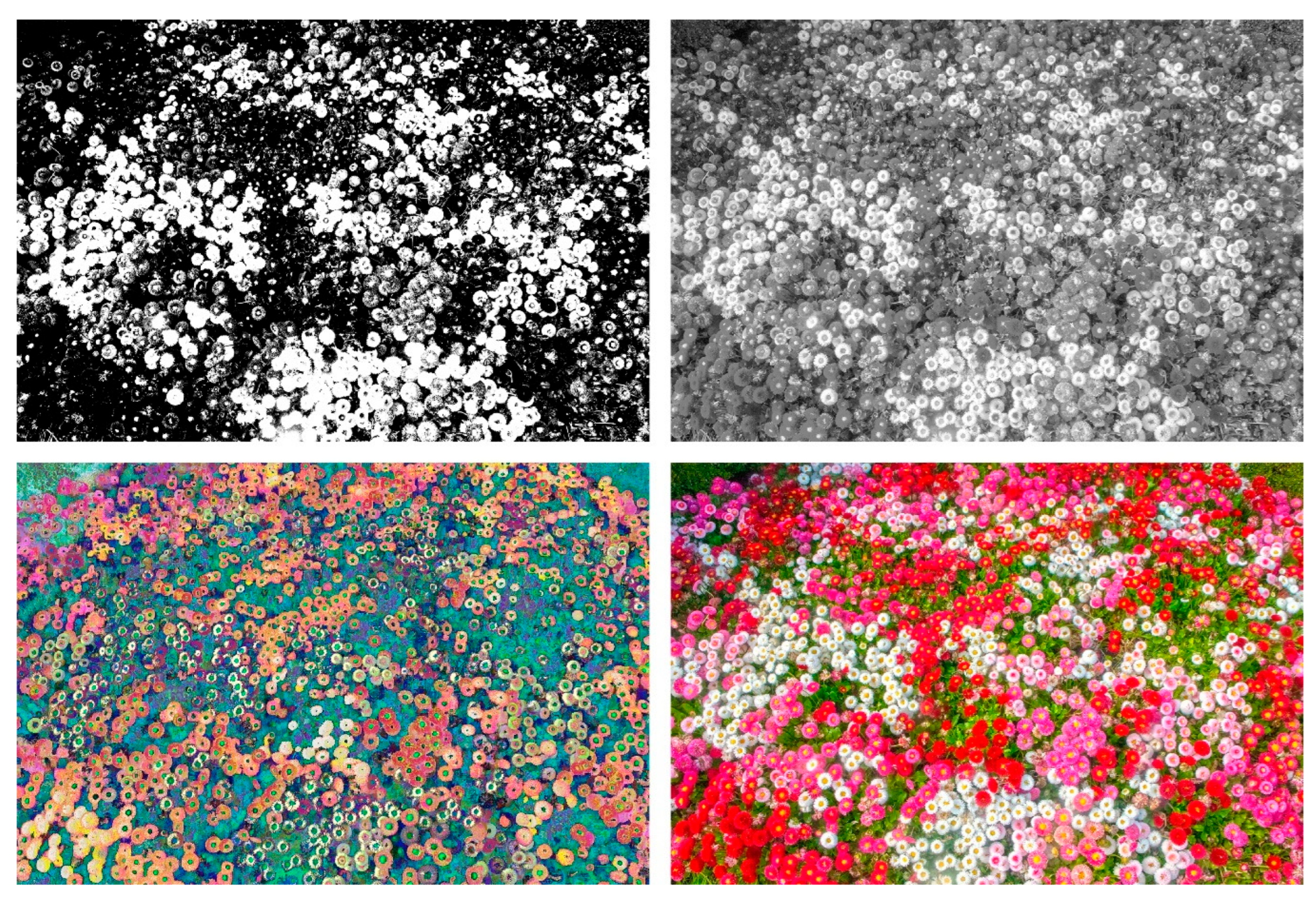
Figure 2.
The measurement space of the spectral fractal dimension (Figure 7 of [18]). Illustration of spectral boxes (216 = 65,536) used during SFD calculation of 16-bit images. The coordinate system formed by the independent axes (image band 1, 2, 3) forms the spectral space. Each pixel is assigned to the spectral boxes based on the values of the pixels occurring in the same position in the image.
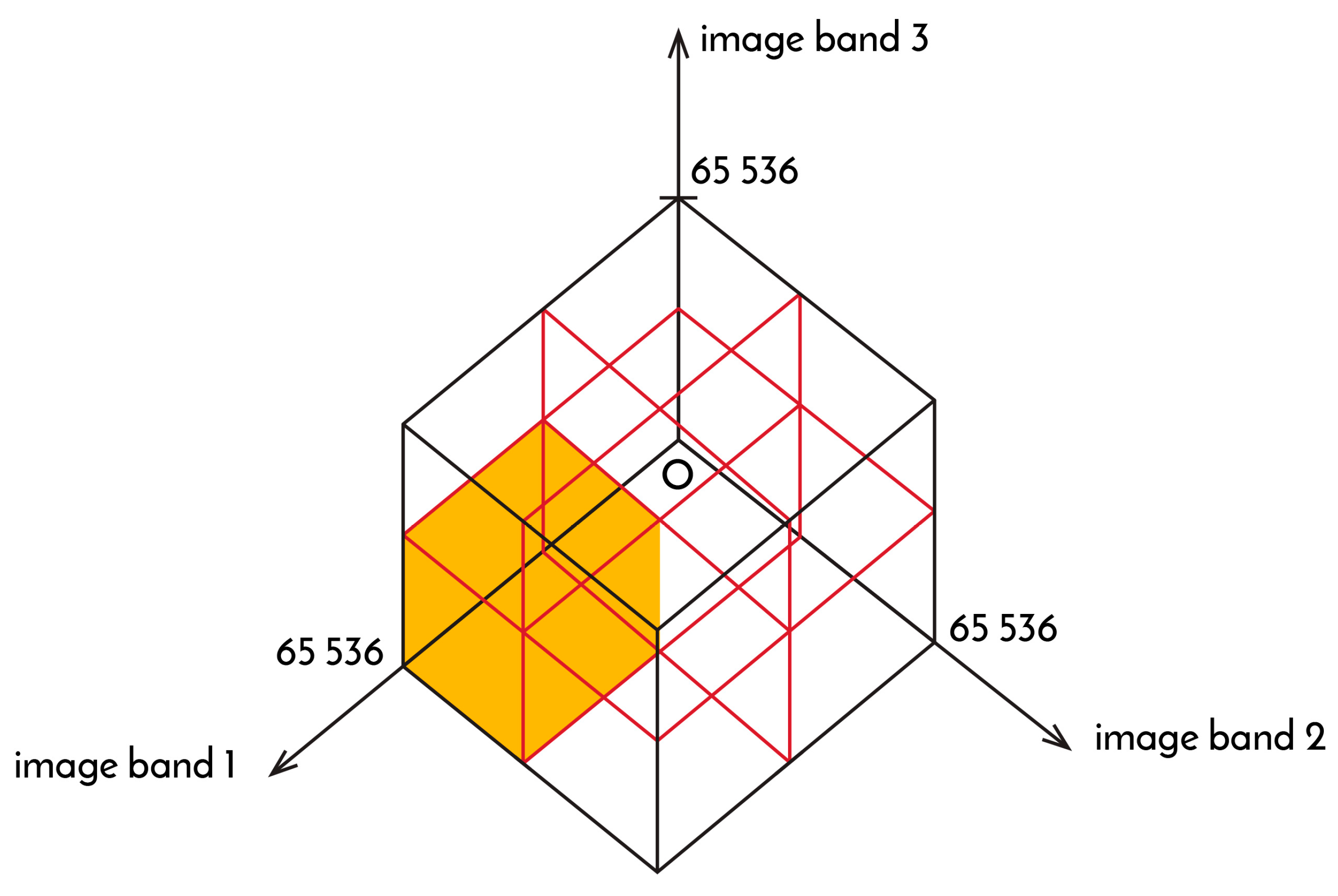
Figure 3.
Figure 2 of [22] shows the image data of sensors placed in four independent spectral ranges, but in a single camera array, which are respectively: MS-R—Red band of 4-band orthophoto, MS-G—Green band of 4-band orthophoto, MS-RE—Red-Edge band of 4-band orthophoto and MS-NIR—NIR band of 4-band orthophoto. Images were taken with the DJI M3 Multispectral camera array, at a flight altitude of 100 m relative to the take-off point (GND), on 29 May 2024.
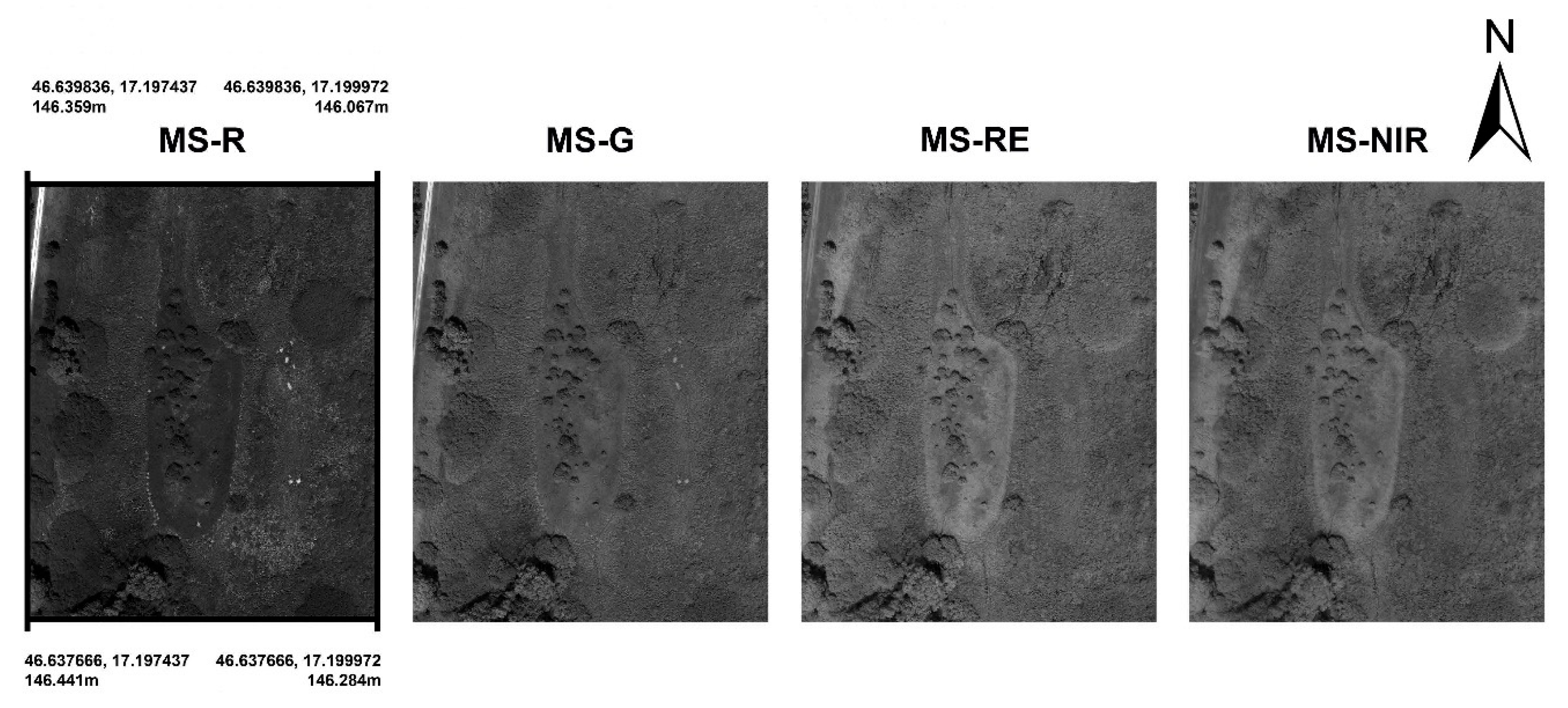
Figure 4.
EW-SFD values of images obtained by band mixing the images in Figure 3.
Figure 4.
EW-SFD values of images obtained by band mixing the images in Figure 3.
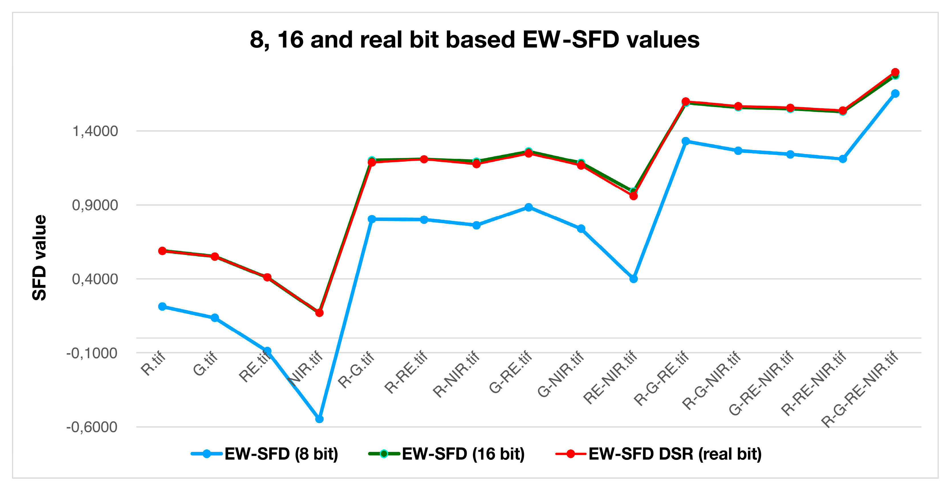
Figure 5.
Figure showing the potato tubers of the entire database. Based on the values measured based on relations (5) and (9) (Table 3), the separation gives significant results for the varieties of the entire database.
Figure 5.
Figure showing the potato tubers of the entire database. Based on the values measured based on relations (5) and (9) (Table 3), the separation gives significant results for the varieties of the entire database.

Figure 6.
Table describing the particles of matter in the Standard-model. The original file was used without modification, which can be found below.: https://commons.wikimedia.org/wiki/File:Standard_Model_of_Elementary_Particles.svg.
Figure 6.
Table describing the particles of matter in the Standard-model. The original file was used without modification, which can be found below.: https://commons.wikimedia.org/wiki/File:Standard_Model_of_Elementary_Particles.svg.
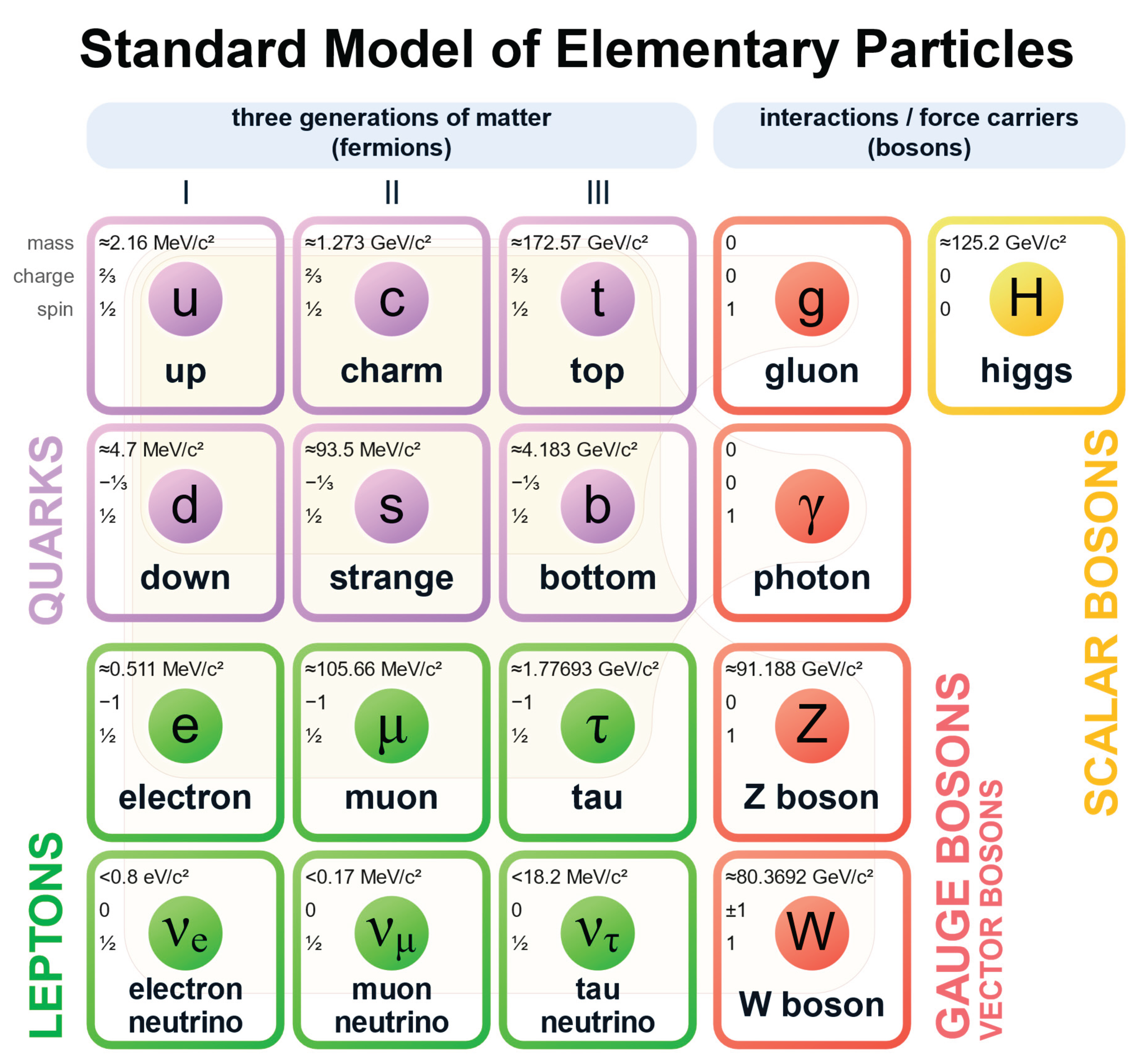
Table 4.
MCS spatial values based on the Standard-model.
| Image layer type | Values | Number of different values | Color space /bit/ |
|---|---|---|---|
| Mass | 0 MeV/c2, 0,8 eV/c2, 0,17 MeV/c2, 0,511 MeV/c2, 2,16 MeV/c2, 4,7 MeV/c2, 18,2 MeV/c2, 93,5 MeV/c2, 105,66 MeV/c2, 1,273 GeV/c2, 1,77693 GeV/c2, 4,183 GeV/c2, 80,3692 GeV/c2, 91,188 GeV/c2, 125,2 GeV/c2, 172,57 GeV/c2, | 16 | 4 |
|
Charge |
-1, -1/3, 0, 2/3, 1 |
5 |
3 |
|
Spin |
0, ½, 1 |
3 |
2 |
|
MCS color |
24 |
24 |
9 |
Disclaimer/Publisher’s Note: The statements, opinions and data contained in all publications are solely those of the individual author(s) and contributor(s) and not of MDPI and/or the editor(s). MDPI and/or the editor(s) disclaim responsibility for any injury to people or property resulting from any ideas, methods, instructions or products referred to in the content. |
© 2025 by the authors. Licensee MDPI, Basel, Switzerland. This article is an open access article distributed under the terms and conditions of the Creative Commons Attribution (CC BY) license (http://creativecommons.org/licenses/by/4.0/).
Copyright: This open access article is published under a Creative Commons CC BY 4.0 license, which permit the free download, distribution, and reuse, provided that the author and preprint are cited in any reuse.


