
Submitted:
22 September 2025
Posted:
23 September 2025
You are already at the latest version
Abstract
Fractional heat conduction models extend classical formulations by incorporating fractional differential operators that capture multiscale relaxation effects. In this work, we introduce an electrical analogy that represents the action of these operators via generalized longitudinal impedance and admittance elements, thereby clarifying their physical role in energy transfer: fractional derivatives account for the redistribution of heat accumulation and dissipation within micro-scale heterogeneous structures. This analogy unifies different classes of fractional models—diffusive, wave-like, and mixed—as well as distinct fractional operator types, including the Caputo and Atangana–Baleanu forms. It also provides a general computational methodology for solving heat conduction problems through the concept of thermal impedance, defined as the ratio of surface temperature variations (relative to ambient equilibrium) to the applied heat flux. The approach is illustrated for a semi-infinite sample, where different models and operators are shown to generate characteristic spectral patterns in thermal impedance. By linking these spectral signatures of microstructural relaxation to experimentally measurable quantities, the framework not only establishes a unified theoretical foundation but also offers a practical computational tool for identifying relaxation mechanisms through impedance analysis in microscale thermal transport.
Keywords:
fractional heat conduction
; subdiffusion
; wave-like heat transfer
; electro-thermal analogy
; complex heat capacity
; complex thermal conductivity
1. Introduction
The classical theory of heat conduction, formulated in the early 19th century, is one of the most widely used models in physics and engineering [1]. For more than 150 years, it has been successfully applied in various domains—from civil engineering and geophysics to electronics, biomedicine, and the development of modern experimental techniques based on the photothermal effect [2,3,4,5,6,7]. This theory is based on the principle of energy conservation and on Fourier’s constitutive relation between the temperature gradient and the heat flux, a phenomenological relation consistent with the Second Law of Thermodynamics [1]. This formulation leads to a diffusion-type partial differential equation (a parabolic PDE), which describes the temporal and spatial distribution of temperature variations (relative to the ambient temperature) in a system [1,8].
Despite its wide applicability, the classical model exhibits significant limitations in explaining heat transfer in media with complex internal structures such as polymeric [9,10,11,12,13] or glassy materials [14,15,16] and biological tissues [17,18,19,20,21], where anomalous diffusion and wave-like effects emerge as a consequence of the complex dynamics of internal degrees of freedom. To overcome this shortcoming, various fractional models have been developed [22,23,24,25,26,27,28,29].
The literature generally distinguishes several classes of fractional models of heat conduction. Some are derived from probabilistic approaches, most notably the Continuous Time Random Walk (CTRW) framework [28,29,30,31,32,33,34], which describes subdiffusion type of anomalous diffusion through a nonlinear dependence of the mean-square displacement on time, , . Most fractional models, however, are based on phenomenological considerations. Among them there are formulations that introduce the concept of inertia in heat flow via fractional time-delayed heat flux [26,35,36] enabling the description of wave-like features of heat transfer. Besides, there are fractional dual phase lag models [37,38,39] that introduce the influence of the thermal displacement in time-delayed heat flux enabling description wave-like and anomalous diffusive effects. Another important group consists of time-fractional telegraph models, often referred to as Generalized Cattaneo equations [32], which capture both subdiffusive and superdiffusive anomalous effects as well as wave-like propagation of thermal disturbances by replacing the integer time differential operator with fractional operators [40,41,42,43,44]. Finally, some formulations are derived from Hamilton–Jacobi-type formalisms [45,46], offering alternative perspectives on fractional thermal transport.
However, to the best of our knowledge, the literature still lacks a unified framework for fractional heat-conduction models that would enable systematic comparison and evaluation of their thermodynamic consistency, treatment of irreversibility and dissipation, and their macroscopic, experimentally measurable consequences. Establishing such a framework would be highly valuable, both for advancing the fundamental understanding of internal relaxation processes in complex materials and for interpreting experimentally observed phenomena—such as anomalous diffusion or wave-like effects.
In this work, we demonstrate that identifying two distinct types of memory effects—kinetic memory and inertial memory in energy balance—provides a framework that explains the thermodynamic consistency of fractional models by introducing concept of complex heat capacity and complex thermal conductivity. This motivates the use of analogical methods, in particular electrical analogies [47,48,49,50,51,52], which provide both a powerful and intuitive framework to clarify the role of fractional differential operators and to enable systematic comparison of different fractional models. We further show that this analogy establishes a general platform for solving spatiotemporal temperature distributions in media where heat conduction is governed by time-fractional models. The framework not only yields deeper physical insight into how different internal relaxation processes related to material memory affect energy storage and dissipation, but also facilitates analytical and numerical solutions through the definition of thermal counterparts to the propagation coefficient (thermal wave vector) and to the characteristic impedance (thermal impedance).
Within this framework, we analyze the boundary value problem of a photothermally excited sample using three groups of fractional theories with time-fractional differential operators. The derived expressions allow the determination of surface temperature variations, which is particularly relevant for the interpretation of experimental results in photothermal techniques and other methods based on thermal wave propagation. Special attention is devoted to the role of different fractional operators, with the Caputo [53] and Atangana–Baleanu (in the Caputo sense) [54,55] operators analyzed in detail, emphasizing their distinct implications for the evolution of surface temperature variations.
The structure of the paper is as follows. After this introductory section, Section 2 briefly reviews the mathematical properties of the Caputo (C) and Atangana–Baleanu in the Caputo sense (ABC) operators. Section 3 introduces the heat conduction model in the Laplace domain, which, by introducing two new parameters—complex heat capacity and complex thermal conductivity—encompasses all fractional heat conduction models. The analogy with current and voltage propagation in transmission lines is then discussed, and the concept of thermal impedance is defined, describing thermal disturbance propagation in direct relation to complex heat capacity and thermal conductivity. In Section 4, based on this analogy, thermal impedance is analyzed as an experimentally measurable thermal property, with spectral characteristics of a semi-infinite sample studied for three groups of fractional theories and two types of fractional operators (C and ABC). Finally, Section 5 summarizes the main conclusions and highlights the implications of the results for the interpretation of photothermal experiments and for the further development of fractional heat conduction theories.
2. Fractional Differential Operators Caputo and Atangana-Balenau
Fractional calculus extends the classical notions of differentiation and integration to non-integer orders [56,57,58] and has proven especially powerful for describing systems with long-term memory and temporal nonlocality [27]. These features are essential when modeling anomalous transport of mass, energy, or charge, where conventional integer-order equations often fail to capture the underlying dynamics.
In this work, we focus on two types of time-fractional operators. The first is the Caputo operator [53,57,58], widely used in physical applications because it incorporates initial conditions in a straightforward manner. The second is the Atangana–Baleanu operator in the Caputo sense (ABC) [54,55], which employs nonsingular kernels and provides a smoother representation of memory effects across multiple time scales.
From a physical perspective, the Caputo operator is well suited for processes governed by persistent long-term memory, while the ABC operator can describe more intricate transient responses with gradually fading memory. Both operators are therefore highly relevant for modeling transport in heterogeneous and structurally complex systems such as neural tissue, cell membranes, and disordered porous media.
2.1. Caputo Fractional Derivative
The Caputo fractional derivative of order α∈(0,1) for a sufficiently smooth function f(t) on the interval [0,T] is defined as
where Γ(⋅) denotes the Gamma function [59].
This operator introduces a power-law memory with a singular kernel, meaning that the present state of the system depends on its entire history, weighted by a slowly decaying function of the form (t−τ)−α. Such long-tail memory effects are characteristic of subdiffusive processes and anomalous transport phenomena, and they can be associated with internal degrees of freedom that relax slowly.
An important advantage of the Caputo derivative is that it allows the formulation of initial conditions in terms of integer-order derivatives of f(t), which is consistent with physical intuition and simplifies both numerical implementation and analytical interpretation. In the limiting cases,
The Laplace transform of the Caputo derivative is given by
where
Since the Laplace transform of the Caputo operator is expressed in terms of the function value and its integer-order derivatives at the initial time—quantities that are typically known or can be determined from physical arguments—this formalism enables an efficient analysis of frequency-domain characteristics and provides a convenient tool for solving fractional differential and partial differential equations in which Caputo-type operators appear.
2.2. Atangana–Baleanu (AB) Fractional Operator
The Atangana–Baleanu (AB) operator is a more recent approach to fractional modeling of dynamical systems with memory. Unlike the Caputo operator, it employs a non-singular kernel based on the Mittag–Leffler (ML) function [60,61,62]. This non-singular kernel eliminates the physically questionable singularities at the initial moment and enables the description of complex transitional relaxation regimes that cannot be captured by pure power-law laws.
To allow the use of classical initial conditions expressed in terms of integer-order derivatives, the AB operator is used here in the Caputo sense (the so-called ABC operator), which represents a significant practical advantage for solving real-world problems.
For a sufficiently smooth function f(t), the AB and ABC fractional derivatives of order α∈(0,1) are defined as
where Eα(⋅) is the one parmeter Mittag–Leffler function and B(α) is a normalization coefficient [60].
The kernel of this operator is a smooth function, which implies that the system possesses exponentially tempered memory—in contrast to the long-tailed power-law memory of the Caputo operator. This property makes it particularly suitable for describing systems with multiple characteristic time scales and intermediate relaxation regimes, phenomena often encountered in biological tissues, polymers, and amorphous materials.
In the limiting cases, the AB operator reduces to the same integer-order forms as the Caputo operator:
The Laplace transform of the ABC operator is given by
which highlights a relaxation dynamics with a spectral response modified by an exponential-type factor, in contrast to the pure power-law spectrum of Caputo-type models.
2.3. Comparative Remarks: Caputo vs. Atangana–Baleanu Operators
Both the Caputo and the Atangana–Baleanu (ABC) operators generalize the classical derivative to non-integer orders, but they differ in the nature of their memory kernels and in the type of physical processes they are most suitable to describe, what is illustrated in Table 1.
In summary, the Caputo operator provides a framework for describing systems with persistent long-term memory and anomalous subdiffusive dynamics, while the ABC operator offers additional flexibility for modeling materials and processes characterized by tempered memory effects and multiple characteristic time scales.
3. Generalized Fractional Heat Conduction Theories and Analogy with Voltage and Current Propagation in an Transmission Line
3.1. Theoretical Framework of Classical Heat Conduction via Constitutive Relations and Energy Conservation
From a thermodynamic perspective, the first law of thermodynamics (energy balance) for a system excited by an external energy source can be written as [63,64]:
together with the constitutive relations:
Here, denotes the Dirac delta function, f(t) is a dimensionless temporal profile of the heat flux source of intensity S0 [W/m³], u(x,t) [J/m³] represents the change in internal energy density associated with temperature variations [K], [W/m²] is the heat flux. Tempetarure variations is defined by where is the initial temperature of the system in equilibrium with ambient and ambiental temperature (before the action of thermal source].
In classical heat conduction, both constitutive relations are linear and temporally local:
where is volumetric heat capacity [J/(K•m³)], is mass density [kg/m³], is specific heat at constant pressure [J/(K•kg)], and k is thermal conductivity [W/(m•K)].
Substituting Eq (11) and Eq (12) into Eq (8) yields the classical diffusion equation:
Eq (13) predicts that temperature disturbances propagate instantaneously across the system, implying infinite speed of heat propagation [65,66,67,68,69,70]. This unphysical result arises from the temporal locality of the constitutive relation in Eq (12), which assumes that the heat flux at a given point depends only on the temperature gradient at the same point and time, neglecting any effects from previous times—i.e., the inertial memory of energy carriers in the system [65,67,68].
Mathematically, accounting for these memory effects leads to wave-like or damped wave models instead of the parabolic diffusion description of classical theory, allowing for finite-speed propagation [65,66,67,68,69,70]. However, temporal nonlocality in the heat flux relation alone does not resolve another limitation of classical theory: it still treats system evolution as an ergodic process in phase space [10,71,72].
From a thermodynamic viewpoint, with the first law (Eq 8) and a local constitutive link between internal energy and temperature (Eq11), the temperature gradient acts as the sole affinity driving the system toward global equilibrium, regardless of energy carrier inertia [10] . It means that hyperbolic theories, like the classical diffusion equation, assume that infinitesimal system volumes instantaneously reach local equilibrium. In other words, temporal locality of constitutive relation between density of internal energy and scalar temperature field (Eq 11) neglects the kinetic memory of the system.
From these considerations, we can distinguish two types of memory: inertial memory: associated with temporal nonlocality in the relation between heat flux and temperature gradient, giving rise to wave-like propagation and kinetic memory associated with temporal nonlocality in the relation between internal energy and temperature, producing an additional thermodynamic driving force that guides the system toward global equilibrium, not necessarily through a sequence of local equilibrium states [10,71,72,73,74,75].
This distinction provides a foundation for fractional heat conduction models, where temporal nonlocality of the energy conservation law arises naturally from introducing fractional derivatives in one or both constitutive relations (Eq 9 and Eq 10).
3.2. Fractional Heat Conduction Theories
The temporal nonlocality of the constitutive relation in Eq (2), reflecting the kinetic memory of the system, can be modeled by introducing a fractional differential operator:
Here, the memory kernel of the fractional operator is a dimensionless function describing the kinetic memory, and is the fractional volumetric heat capacity with dimensions [Jsα/m3K].
Substituting Eq (14) for Eq (9) in the energy conservation law (Eq 8) leads to a nonlocal energy balance, which together with Eq (10) gives the first type of fractional heat conduction theory, mathematically expressed as a linear fractional diffusion equation:
Typically, the Caputo fractional derivative is used (Section 2.1), while more recently the ABC derivative has become popular (Section 2.2). Eq (15) with Caputo type of operator corresponds to subdiffusion, which can also be derived from the stochastic CTRW approach, where the mean squared displacement of energy carriers is nonlinearly dependent on time [32,33]. This links anomalous diffusion effects to the kinetic memoryof the system.
The effect of inertial memory can similarly be introduced in the relation between the temperature gradient (thermodynamic force) and its conjugate heat flux (Eq 10) via a fractional differential operator:
Substituting Eq (16) into Eq (8), while assuming a local relation between internal energy change and temperature (Eq 11), yields the second type of fractional heat conduction theory:
Analogous to the hyperbolic Cattaneo–Vernotte equation [76,77], Eq (17) can not describe subdiffusion or local-nonequilibrium movement of the system towar global equilibrium with surrounding. Therefore, inertial memory is associated only with sharper thermal wavefronts, superdiffusive behavior, and finite-speed propagation, i.e., wave-like effects.
If both constitutive relations (Eq 9 and Eq 10) are generalized using fractional operators (Eq 14 and Eq 16), the resulting theory incorporates both kinetic and inertial memory effects, allowing for the description of anomalous diffusion and wave-like propagation simultaneously, as well as local non-equilibrium movement of the system across phase space:
From this point of view, it is important to note that fractional DPL models [37,38] introduce inertial memory explicitly and kinetic memory implicitly, via complex nonlocal relations between heat flux, temperature gradient and thermal displacement. They can be linked to Eq (18) by choosing appropriate fractional operators or combining fractional derivatives with phase delays between generalized thermodynamic forces (temperature gradient and scalar temperature field) and their conjugate fluxes (heat flux and internal energy).
Similarly, fractional telegraph-equation models (known in literature as Generalized Cattaneo Equations (GCE) [32] or models derived via Hamilton–Jacobi formalism [45,46] follow the same thermodynamic consistency and could be considered from point of view memory effects caused kinetic and inertial memory of the system.
Interestingly, Eq. (15), which represents a fractional generalization of the internal energy–temperature relation, reduces to the classical Debye relaxation theory when the power-law kernel (Caputo) or Mittag–Leffler kernel (ABC) is replaced by an exponentially decaying kernel. In this case, a phase lag appears between the internal energy density and the scalar temperature field, a feature commonly used to describe thermal propagation in glasses and amorphous materials [15].
Similarly, Eq. (17) reduces to the Cattaneo–Vernotte hyperbolic model when the convolution kernel in Eq. (9) is replaced by an exponentially decaying kernel [67,68]. The Cattaneo–Vernotte model was originally developed as a generalization of the second-sound model of heat conduction (undamped wave propagation) [78] at low temperatures close to liquid helium temperature [79,80,81,82], and it has more recently been applied to 2D materials in the 100–200 K range [83,84].
3.3. Generaliyed Heat Conduction Theories with Fractional Temporal Operators in Laplace Space and Electrical Analogy
In this subsection, an electrical analogy is introduced, which allows us to relate thermal memory effects to complex elements in an electrical circuit (memory resistors, memory capacitors, and memory inductor) and to understand the physical meaning of fractional operators in the thermodynamic context.
It will be shown that these operators introduce a frequency-dependent redistribution of energy accumulation and dissipation within a thermally excited system, strongly influencing the temperature evolution and all phenomena connected with thermal changes, which underlie many calorimetric and photothermal experimental techniques [2,3].
Electro-Thermal Analogy
By applying the Laplace transform to Eq (15), and assuming , we obtain a linear differential equation in the complex domain, describing the first type of fractional heat conduction:
where denotes the Laplace transform of f(t). The complex heat capacity in Eq (19) is defined as:
As it can be seen from Eq20, the spectrum of complex heat capacity depends on the spectral properties of memory kernel of fractional differential operator, . For the Caputo derivative, the complex heat capacity is:
while for the ABC derivative, it is:
The real and imaginary parts are obtained by mapping from the s-plane to the jω axis (j is the imaginary unit) and depend on the type of fractional operator. For Caputo and ABC operators, the real and imaginary parts of complex heat capacity are given by:
where .
Similarly, applying the Laplace transform to Eq (17), assuming the system was initially at equilibrium (), yields the equation describing the second type of fractional heat conduction:
where the complex thermal conductivity is
For Caputo and ABC operators, complex thermal conductivities are given by:
Real and imaginary parts of complex thermal conductivity for Caputo and ABC operators are:
Applying the Laplace transform to Eq (18) gives:
where complex heat capacities and complex thermal conductivities for different operators are given by Eq 21, 22, and Eq 25, Eq 26 and their real and imaginary parts by Eqs 23, 24 and Eq 31, 32 for Caputo type of operator and Eqs 25, 26 and Eq 33, 34 for ABC type of operator.
Each of the fractional theories given by Eq (12), Eq (20), and Eq (28) is formally analogous to the propagation of current and voltage in an electrical line, where: the energy conservation law (first law of thermodynamics) corresponds to Kirchhoff's current law and the constitutive relation between heat flux and temperature gradient corresponds to Kirchhoff's voltage law (spatially local and global), illustrating the generality of the analogy.
In this analogy, temperature variation corresponds to potential difference in an infinitesimal volume or between two infinitesimal volume , heat flux corresponds to current entering the infinitesimal volume or leaving the infinitesimal volume due to an external source and the formation of a temperature gradient , and internal energy density corresponds to charge storage in a spatially local volume. The relations between temperature variations and heat flux are given by longitudinal impedance and longitudinal admittance, what is illustrated in Figure 1. (compare to discret model in [90,91].
The longitudinal impedances and admittances differ for each type of theory.
For the first group of fractional theories (Eq 19), that include only kinetic memory effets, we obtain real longitudinal impedance and complex longitudinal admittance:
For second group of fractional theories (Eq 27) that include only inertial memory effect we obtain
For third group of fractional theories (Eq 35) that include both kinetic and inertial memory effect we obtain:
In summary, introducing the effect of kinetic memory leads to the first class of theories, which describe media with real thermal conductivity but complex heat capacity. Considering only inertial memory gives rise to the second class of theories, which describe media with real heat capacity but complex thermal conductivity. Finally, when both types of memory are taken into account, one arrives at the third class of theories, which describe heat conduction in media characterized by both complex heat capacity and complex thermal conductivity.
Compared with the classical parabolic diffusion theory, it can be concluded that in the classical model of heat conduction—which assumes purely real heat capacity and thermal conductivity—the real part of the heat capacity describes reversible energy storage in fast, localized internal modes (such as molecular rotations, bond stretching, or intramolecular vibrations). In contrast, the real part of the thermal conductivity accounts for irreversible energy dissipation along the flow direction, primarily through scattering of collective carriers such as phonons or related excitations.
When kinetic memory is introduced (Eqs. 36, 37), an additional dissipative channel appears, represented by the imaginary part of the heat capacity. Microscopically, this corresponds to local vibrational modes that become trapped and partially converted into metastable states, thereby feeding the entropic reservoir.
By contrast, inertial memory contributes a new reversible accumulation channel, expressed by the imaginary part of the thermal conductivity (Eqs. 38, 39). This term reflects transient energy storage within the heat flux itself, arising from long-lived collective modes. Together with standard storage in the local volume, this mechanism allows oscillatory exchange of energy between different types of internal degrees of freedom, ultimately enabling the formation of a propagating temperature wavefront with finite speed.
In summary, kinetic memory introduces additional irreversible dissipation within each local volume, while inertial memory introduces reversible transient accumulation in the energy flux. The full picture thus combines scattering, metastable-state formation, and oscillatory energy transfer between distinct internal degrees of freedom.
A comparison with generalized non-fractional models of heat conduction—such as the Debye relaxation model, the hyperbolic Cattaneo model, and the Dual-Phase-Lag (DPL) model—shows that exponentially decaying (fading) kinetic and inertial memory produces effects similar to those obtained with fractional operators. These include additional dissipative channels in the local volume or reversible energy accumulation in the heat flux, associated with trapped vibrational modes and oscillatory energy exchange between distinct internal degrees of freedom. The essential difference, however, lies in the way memory is represented. In non-fractional models, exponentially decaying kernels describe fading finite-time memory, characterized by a single relaxation delay between thermodynamic forces and their conjugate fluxes. By contrast, fractional operators introduce complex frequency-dependent equivalent electrical elements—analogous to those in dielectric Cole–Cole models [92]—that capture long-tailed or tempered memory effects involving multiple characteristic time scales. In this way, they describe hierarchical multiscale relaxations of internal degrees of freedom and the multiscale lifetimes of collective modes, which together govern the complex dynamics of thermal conduction in structurally heterogeneous materials.
Finally, the table review of this consideration is given below (Table 2).
4. Application of Electro-Thermal Analogy in Fractional Heat Conductions Problems and Calculated Surface Temperature Variations
Heat conduction problems in practical experiments can be efficiently addressed using the electro-thermal analogy introduced in Section 3. In this analogy (Figure 1), the heat conduction equations can be solved similarly to wave propagation problems in a transmission line, using two parameters that govern this propagation: the propagation coefficient (wave vector) and the characteristic impedance of the transmission line [6,68,93,94,95].
In this paper, we solve the problem of heat propagation and calculate the surface temperature variations by applying electro-thermal analogy and using the transfer function concept, illustrating the efficiency of this approach for analyzing fractional memory effects and, consequently, the complex dynamics of internal degrees of freedom in experimentally measured signals from biological membranes, tissues, glassy, and polymeric materials.
4.1. The Mathematical Description of the Problem
To solve the heat conduction problem and enable practical application in thermal experiments, based on the analogy shown in Figure 1, heat conduction can be described by the following relations:
Here, the influence of an external energy source is described through the boundary condition at x=0. The excitation of the sample can be represented either as an analog current source when the excitation is an external heat flux, as in photothermal methods:
or as an analog voltage source when the excitation is a temperature variation at the sample surface:
In the above equations, denotes the Laplace transform of a dimensionless time-dependent function describing the temporal evolution of the excitation, the variation of surface temperature relative to the equilibrium temperature, and S0 the excitation heat flux.
Based on Eqs. (42) and (43), the propagation coefficient (wave vector) and the characteristic thermal impedance can be defined as:
In experimental measurements, only the heat flux or surface temperature variations at the sample boundary are usually known (either directly or indirectly). Therefore, it is particularly important to determine these quantities, rather than the complete space–time distribution. Using the analogy shown in Figure 1 and the expressions (46) and (47), the relation between surface variations of temperature and heat flux can be determined through the equivalent two-port network (T or Π network) shown in Figure 2, where the impedances of the equivalent circuits can be expressed via the propagation coefficient (Eq. 46) and the characteristic thermal impedance (Eq. 47).
The surface temperature variations at the boundary subjected to an external heat flux, as in PT methods, can be described by:
where denotes the transfer function of the system (equivalent impedance). This function depends on the thermal properties of the sample (complex heat capacity and complex thermal conductivity), on the boundary condition at x=L (the characteristic thermal impedance of the semi-infinite environment), as well as on the temporal dependence of the excitation. Variable L represents the thickness of the sample.
The heat flux variations at the surface excited by a time-dependent temperature change (as in AC calorimetric methods) can be described by:
where denotes the transfer function of the system (equivalent admittance). Similar to , it depends on the thermal properties of the sample (complex heat capacity and complex thermal conductivity), the boundary condition at x=L (the thermal impedance of the surroundings), and the temporal form of the excitation.
In the following, we will analyze the surface temperature variations of a semi-infinite sample.
4.2. Surface Temperature Variations of a Semi-Infinite Sample and Spectral Properties of the Characteristic Thermal Impedance
For an infinitely long sample excited by a heat flux that is uniform across its entire surface, as in photothermal methods [93], the boundary conditions are:
Starting from Eqs. (48) and (49) and Figure 2, the thermal impedance of a semi-infinite sample is equal to the characteristic thermal impedance of the material [68]. In that case, the equivalent electrical scheme is reduced to one illustrated in Figure 3.
According to Figure 3, the surface temperature variations of a semi-infinite sample can be expressed as:
As seen from Eq. (54), these surface temperature variations are modeled as the system’s response to a time-dependent excitation applied at the sample surface. The transfer function is determined by the characteristic thermal impedance of the excited system (Eq. 45), which depends on both the complex thermal conductivity and complex heat capacity. Each of the fractional theories considered predicts different frequency-dependent characteristics of this thermal impedance. Moreover, within each theory, the choice of fractional differential operator (Eqs. 28–33) also influences the frequency response of the transfer functions.
The temporal evolution of these surface responses can be obtained by calculating the inverse Laplace transform of Eq. (54) for each fractional theory. The resulting response depends not only on the chosen theory and the type of fractional operator but also on the temporal form of the excitation signal [6,49,64].
In the following discussion, we analyze the spectral properties of the thermal impedance for each fractional theory, and for different fractional operators within each theory. This analysis is equivalent to studying the spectral properties of the Green’s function for surface temperature variations, since the Green’s function fully characterizes the system’s temporal response, independent of the specific excitation
Starting from Eqs. (28–33) and Eq. (45), and transforming from the Laplace domain (s) to the frequency domain (jω), one can derive expressions for the characteristic thermal impedance of systems with long-tailed or tempered memory.
The first group of fractional theories, for both Caputo and Atangana–Baleanu (ABC) types of fractional operators, predicts the following spectral dependence of the thermal impedance:
For the second group of theories, the spectral characteristics of the characteristic thermal impedance for Caputo and ABC operators are given as:
Finally, for the third group of fractional theories, the corresponding models of the characteristic thermal impedance for Caputo and ABC operators are:
or their combinations, e.g., when the kinetic memory is represented by a long-tail memory (Caputo-type operator) while the inertial memory is represented by tempered memory (the ABC-type operator) (Eq. 61), or in other combinations (Eq. 62):
4.3. Analyzis and Disscussion
The characteristic thermal impedance predicted by the first group of theories (Eqs. 55 and 56) that consider only fractional kinetic memory reduces to the characteristic thermal impedance predicted by the classical parabolic diffusion theory of heat conduction for . The modulus of this impedance tends to infinity when and asymptotically approaches zero when , as [68]. The phase of the characteristic thermal impedance is constant (frequency-independent) in this case and indicates that, as in the classical diffusion theory, there exists a phase shift between the excitation heat flux and the surface thermal variations, which is equal to , and independent of the type of fractional operator.
When in Eq. 55, the characteristic thermal impedance predicted by the fractional model from the first group (complex thermal capacitance and real thermal conductivity) with the Caputo-type operator yields a constant and real thermal impedance over the entire frequency range, i.e., without any phase shift. In other words, in this case the characteristic thermal impedance reduces to the equivalent thermal resistance equal to .
If, within the first group of fractional theories, the ABC operator is used instead of the Caputo operator, then according to Eq. (56) for , one obtains a frequency-dependent thermal impedance
When , the modulus of this impedance tends to infinity, while for , the modulus of this impedance tends to a finite constant value different from zero, . The phase of the characteristic thermal impedance is also frequency-dependent and varies from for to when , indicating that the ABC-type operator at high frequencies essentially predicts a phase lag of surface thermal variations that is nearly the same as in the classical model, while at low frequencies it predicts for larger phase lag.
Based on the above considerations, it can be concluded that the differences between Caputo and ABC-type operators are reflected in the amplitude and phase spectra of the thermal impedance. In other words, variations in the dynamics of multiscale relaxations within spatially local modes manifest as distinct signatures in the characteristic thermal impedance of the sample. When the order of the fractional operator approaches one, these differences diminish, and the characteristic thermal impedance predicted by the first group of fractional models converges toward that predicted by classical diffusion theory.
The characteristic thermal impedance predicted by the second group of theories (Eqs. 57 and 58), which consider only fractional inertial memory, reduces to the characteristic thermal impedance of the classical parabolic diffusion theory of heat conduction if as well as to that of the first group of fractional theories for .
For , the Caputo-type operator in the second group of theories (Eq. 57) predicts a frequency-dependent characteristic thermal impedance whose modulus tends to infinity when , while for the modulus asymptotically approaches zero as , i.e., this model exhibits a much faster convergence than the classical diffusion model. The phase of the characteristic thermal impedance is constant in this case and equal to , which means that the second group of theories with the Caputo operator predicts that the characteristic thermal impedance behaves as an equivalent frequency-dependent inductance.
The ABC-type operator for in the second group of theories (Eq. 58) predicts an infinite amplitude of the characteristic thermal impedance and a phase equal to at all frequencies. Interestingly, such a characteristic thermal impedance is predicted by undamped wave-type hyperbolic models, such as the second sound model or the hyperbolic Cattaneo–Vernotte model in the limit of infinite thermal relaxation time. These models are associated with long-time inertial memory that does not decay with time [96], and can be microscopically linked to long-lived degrees of freedom that prevent the energy introduced into the system from dissipating into the entropic reservoir, instead allowing its resonant transfer through the system.
In the third group of models, that consider both fractional memory, we analyze only the case in order to examine how different fractional operators affect the complex thermal impedance. In this case, Eqs. (59)–(62) reduce to the following expressions:
From the analysis of Eq. (64) for , it follows that the model with the Caputo operator from the third group predicts the same characteristic thermal impedance as the Caputo operator from the first group of models for (i.e., the characteristic thermal impedance behaves as a frequency-independent equivalent thermal resistance equal to . For , the result coincides with the characteristic thermal impedance obtained in the first group of theories for or in the second group of theories for , namely the same impedance as predicted by the classical diffusion theory. For , the third group of models yields the same characteristic thermal impedance as the second group of theories with the Caputo operator and , which corresponds to a frequency-dependent amplitude of the characteristic thermal impedance, where the modulus tends to infinity when , while for the modulus asymptotically approaches zero as . The phase of the characteristic thermal impedance in this case is constant and equal to .
For the ABC-type operator and , Eq. (65) reduces to Eq. (63), which means that the modulus of the characteristic thermal impedance tends to infinity when while for the modulus approaches a constant value different from zero, . The phase of the characteristic thermal impedance varies from for to when . This is exactly the same behavior of the characteristic thermal impedance as that predicted by the first group of theories with the ABC operator and .
For , Eq. (58) reduces to
which is not equal to the characteristic thermal impedance predicted by either the first group of theories with the ABC operator and , or the second group of theories for , i.e., it does not reduce to the characteristic thermal impedance given by the classical diffusion theory. The only similarity is that, also in this model, the amplitude of the characteristic thermal impedance ranges from infinitely large values when to zero when . This model predicts a complex frequency dependence of the phase of the characteristic thermal impedance for .
For , the ABC operator predicts an infinite amplitude of the characteristic thermal impedance and a constant phase equal to at all frequencies, as in the second group of theories with the ABC operator for , i.e., in the same way as wave-type models (the second-sound model or the hyperbolic Cattaneo–Vernotte model in the limit of infinite thermal relaxation time).
Based on the above considerations, it can be concluded that in the amplitude and phase spectra of the thermal impedance in the third group of theories, a pronounced difference is observed between the effects of the Caputo and ABC operators. Nevertheless, both operators in the third group of models predict that the characteristic thermal impedance reflects the complex dynamics of spatially localized and spatially nonlocal internal degrees of freedom.
If, in the third group of theories, the inertial and kinetic memory are described by different types of fractional operators, for α=β=γ two distinct models of the characteristic thermal impedance are obtained, Eq. (59) and Eq. (60).
If the kinetic memory is described by the Caputo-type operator and the inertial memory by the ABC operator, then from Eq. (66) for the thermal impedance is found to be frequency-independent and real (equivalent to a thermal resistance), identical to the result obtained in the first group of theories with the Caputo operator and . For , this model predicts a complex frequency dependence of the characteristic thermal impedance, whose amplitude tends to infinity when and asymptotically approaches zero when . For , the model predicts an infinite amplitude of the characteristic thermal impedance and a constant phase equal to at all frequencies, just as in the second group of theories with the ABC operator for , or equivalently as in undamped wave-type models, or the third group of theories with the ABC operator and .
If the kinetic memory is described by the ABC operator and the inertial memory by the Caputo operator, then for Eq. (67) yields a characteristic thermal impedance identical to that of the first group of theories with the ABC operator and . For , this model predicts a complex frequency dependence of the characteristic thermal impedance, whose amplitude tends to infinity when and asymptotically approaches zero when . For , this theory predicts a frequency-dependent characteristic thermal impedance whose modulus tends to infinity when and asymptotically decays to zero as , with a constant phase equal to , exactly as in the second group of theories with the Caputo operator when .
Finally, each of the theories—whether involving a single type of fractional operator or a combination thereof—leaves a unique signature in the characteristic thermal impedance. This indicates that thermal impedance spectroscopy can be employed to identify the theory that best captures the dynamics of the internal degrees of freedom in a given material, as well as to monitor the complex dynamics of these internal modes.
5. Conclusions
We unify diverse fractional heat conduction models through the fundamental concepts of kinetic memory and inertial memory, which capture the thermodynamic foundation of fractional models. Building on this unification, we introduce an electrical analogy in which fractional operators are mapped onto complex heat capacity and complex thermal conductivity. This mapping demonstrates that long-living and slowly relaxing internal degrees of freedom govern the redistribution of accumulated and dissipated energy in the excited system.
Within this framework, thermal impedance emerges as an experimentally measurable property directly linked to the complex conductivity and capacity of the material, thereby providing access to the multiscale relaxation dynamics of microscopically heterogeneous systems. Using the case of a semi-infinite sample, we demonstrated how the interplay of kinetic and inertial memory—described by different fractional models and operator types—affects the characteristic thermal impedance.
The analysis shows that each fractional theory, whether involving a single type of fractional operator or a combination thereof, leaves a unique signature in the characteristic thermal impedance. This indicates that thermal impedance spectroscopy can be employed to select the theoretical model that best captures the dynamics of internal degrees of freedom in a given material, as well as to monitor the complex temporal evolution of these internal modes.
Future work may extend this approach to analyze the thermal impedance of finite-length samples and time-domain responses for various combinations of fractional models and operators, enabling deeper insights into the relaxation times of cooperative processes underlying wave-like and anomalous diffusive effects in glassy solids, nanoporous and biological membranes, and biological tissues.
Author Contributions
Conceptualization, S.G.; methodology, S.G.; validation, M.N.P., D.C.; formal analysis, S.G, M.N.P., and D.C.; investigation, S.G, D.C., and M.N.P.; resources, S.G, D.C; writing—original draft preparation, S.G.; writing—review and editing, S.G., M.N.P., D.C..; visualization, D.C..; All authors have read and agreed to the published version of the manuscript.
Funding
This work was supported by the Ministry of Science, Technological Development and Innovation of the Republic of Serbia, Contract No. 451-03-136/2025-03/200017.
Data Availability Statement
The authors declare that the data supporting the findings of this study are available upon reasonable request. The research is theoretical in nature, involving the proposal of a model and the analysis of its results. No databases were used in this study.
Acknowledgments of AI Assistance
We would like to express our gratitude for the assistance received in improving the clarity and coherence of the manuscript. However, it is important to clarify that the authors retain full responsibility for all content, analyses, and conclusions presented in this work. The role of artificial intelligence in this context was limited to providing language enhancement and stylistic suggestions, and does not imply that any part of the manuscript was generated by AI.
Conflicts of Interest
The authors declare no conflicts of interest.
References
- H. S. Carslaw and J. C. Jaeger, Conduction of Heat in Solids. Oxford University Press, USA, 1959.
- S. E. Bialkowski, N. G. C. Astrath, and M. A. Proskurnin, Photothermal spectroscopy methods. John Wiley & Sons, 2019.
- M. Bertolotti and R. Li Voti, “A note on the history of photoacoustic, thermal lensing, and photothermal deflection techniques,” J. Appl. Phys., vol. 128, no. 23, 2020. [CrossRef]
- P. Lishchuk, D. Andrusenko, M. Isaiev, V. Lysenko, and R. Burbelo, “Investigation of Thermal Transport Properties of Porous Silicon by Photoacoustic Technique,” Int. J. Thermophys., vol. 36, no. 9, pp. 2428–2433, 2015. [CrossRef]
- K. Dubyk et al., “Bio-distribution of Carbon Nanoparticles Studied by Photoacoustic Measurements,” Nanoscale Res. Lett., vol. 17, no. 1, 2022. [CrossRef]
- S. P. Galovic et al., “Time-domain minimum-volume cell photoacoustic of thin semiconductor layer. I. Theory,” J. Appl. Phys., vol. 133, no. 24, 2023. [CrossRef]
- S. Galovic, Z. Stanimirovic, I. Stanimirovic, K. Djordjevic, D. Milicevic, and E. Suljovrujic, “Time-resolved photoacoustic response of thin solids measured using minimal volume cell,” Int. Commun. Heat Mass Transf., vol. 155, p. 107574, Jun. 2024. [CrossRef]
- J. Crank, The Mathematics of Diffusion. London: Oxford University Press, 1957.
- B. Wunderlich, Thermal Analysis of Polymeric Materialse. Springer Berlin, Heidelberg, 2005.
- J.-L. Garden et al., “Thermodynamics of small systems by nanocalorimetry: From physical to biological nano-objects,” Thermochim. Acta, vol. 492, no. 1, pp. 16–28, 2009. [CrossRef]
- M. Varma-Nair and B. Wunderlich, “Non isothermal heat capacities and chemical reactions using a modulated DSC,” J. Therm. Anal., vol. 46, no. 3, pp. 879–892, 1996. [CrossRef]
- A. Saiter, H. Couderc, and J. Grenet, “Characterisationof structural relaxation phenomena in polymeric materials from thermal analysisinvestigations,” J. Therm. Anal. Calorim., vol. 88, no. 2, pp. 483–488, 2007. [CrossRef]
- A. Toda and Y. Saruyama, “A modeling of the irreversible melting kinetics of polymer crystals responding to temperature modulation with retardation of melting rate coefficient,” Polymer (Guildf)., vol. 42, no. 10, pp. 4727–4730, 2001. [CrossRef]
- Y. Saruyama, “AC calorimetry at the first order phase transition point,” J. Therm. Anal., vol. 38, no. 8, pp. 1827–1833, 1995.
- N. O. Birge and S. R. Nagel, “Wide-frequency specific heat spectrometer,” Rev. Sci. Instrum., vol. 58, no. 8, pp. 1464–1470, Aug. 1987. [CrossRef]
- P. K. Dixon, “Specific-heat spectroscopy and dielectric susceptibility measurements of salol at the glass transition,” Phys. Rev. B, vol. 42, no. 13, pp. 8179–8186, Nov. 1990. [CrossRef]
- E. P. Scott, M. Tilahun, and B. Vick, “The question of thermal waves in heterogeneous and biological materials.,” J. Biomech. Eng., vol. 131, no. 7, p. 74518, Jul. 2009. [CrossRef]
- K. Mitra, S. Kumar, A. Vedavarz, and M. K. Moallemi, “Experimental Evidence of Hyperbolic Heat Conduction in Processed Meat,” J. Heat Transf., vol. 117, no. 3, 1995. [CrossRef]
- W. Roetzel, N. Putra, and S. Das, “Experiment and analysis for non-Fourier conduction in materials with non-homogeneous inner structure,” Int. J. Therm. Sci., vol. 42, pp. 541–552, Jun. 2003. [CrossRef]
- P. Forghani, H. Ahmadikia, and A. Karimipour, “Non-Fourier Boundary Conditions Effects on the Skin Tissue Temperature Response,” Heat Transf. Res., vol. 46, no. 1, pp. 29–48, Jan. 2017. [CrossRef]
- H. Herwig and K. Beckert, “Experimental evidence about the controversy concerning Fourier or non-Fourier heat conduction in materials with a nonhomogeneous inner structure,” Heat Mass Transf. und Stoffuebertragung, vol. 36, no. 5, pp. 387–392, 2000. [CrossRef]
- L. R. Evangelista and E. Kaminski Lenzi, Fractional Diffusion Equations and Anomalous Diffusion. Cambridge University Press, 2018.
- Q. Zhang, Y. Sun, and J. Yang, “Thermoelastic responses of biological tissue under thermal shock based on three phase lag model,” Case Stud. Therm. Eng., vol. 28, no. July, p. 101376, 2021. [CrossRef]
- M. A. Fahmy and M. M. Almehmadi, “Fractional Dual-Phase-Lag Model for Nonlinear Viscoelastic Soft Tissues,” Fractal Fract., vol. 7, no. 1, 2023. [CrossRef]
- K. Norregaard, R. Metzler, C. M. Ritter, K. Berg-Sørensen, and L. B. Oddershede, “Manipulation and Motion of Organelles and Single Molecules in Living Cells,” Chem. Rev., vol. 117, no. 5, pp. 4342–4375, 2017. [CrossRef]
- F. Mainardi, Fractional Calculus and Waves in Linear Viscoelasticity. Imperial College Press, 2010.
- I. Podlubny, Fractional differential equations: an introduction to fractional derivatives, fractional differential equations, to methods of their solution and some of their applications, vol. 198. elsevier, 1998.
- R. Metzler, J. H. Jeon, A. G. Cherstvy, and E. Barkai, “Anomalous diffusion models and their properties: Non-stationarity, non-ergodicity, and ageing at the centenary of single particle tracking,” Phys. Chem. Chem. Phys., vol. 16, no. 44, pp. 24128–24164, 2014. [CrossRef]
- R. Metzler and J. Klafter, “The Random Walk’s Guide to Anomalous Diffusion: A Fractional Dynamics Approach,” Phys. Rep., vol. 339, pp. 1–77, 2000. [CrossRef]
- J. Klafter and I. M. Sokolov, First Steps in Random Walks, From Tools to Applications. Oxford University Press, 2021.
- R. Metzler and T. F. Nonnenmacher, “Fractional diffusion: Exact representations of spectral functions,” J. Phys. A. Math. Gen., vol. 30, no. 4, pp. 1089–1093, 1997. [CrossRef]
- A. Compte and R. Metzler, “The generalized Cattaneo equation for the description of anomalous transport processes,” J. Phys. A Math. Gen., vol. 30, no. S0305-4470(97)84140–6, pp. 7277–7289, 1997, Online.. Available: papers://97c216e1-ccb4-4efa-9f39-a4a02ccbb270/Paper/p961.
- N. Korabel, R. Klages, A. V Chechkin, I. M. Sokolov, and V. Y. Gonchar, “Fractal properties of anomalous diffusion in intermittent maps,” Phys. Rev. E, vol. 75, no. 3, p. 36213, Mar. 2007. [CrossRef]
- E. Barkai, “CTRW pathways to the fractional diffusion equation,” Chem. Phys., vol. 284, no. 1, pp. 13–27, 2002. [CrossRef]
- M. Caputo and M. Fabrizio, “Applications of new time and spatial fractional derivatives with exponential kernels,” Prog. Fract. Differ. Appl., vol. 2, no. 1, pp. 1–11, 2016. [CrossRef]
- R. Zwanzig, Nonequilibrium Statistical Mechanics. Oxford University Press, 2001.
- M. Kumar, K. N. Rai, and A. Rajeev, “A study of fractional order dual-phase-lag bioheat transfer model,” J. Therm. Biol., vol. 93, p. 102661, Aug. 2020. [CrossRef]
- H. Y. Xu and X. Y. Jiang, “Time fractional dual-phase-lag heat conduction equation,” Chinese Phys. B, vol. 24, no. 3, 2015. [CrossRef]
- T. M. Atanackovic and S. Pilipovic, “On a constitutive equation of heat conduction with fractional derivatives of complex order,” Acta Mech., vol. 229, no. 3, pp. 1111–1121, 2018. [CrossRef]
- A. Somer et al., “The thermoelastic bending and thermal diffusion processes influence on photoacoustic signal generation using open photoacoustic cell technique,” J. Appl. Phys., vol. 114, no. 6, 2013. [CrossRef]
- A. Somer, S. P. Galovic, E. K. Lenzi, A. Novatski, and K. Djordjevic, “Temperature Profile and Thermal Piston Component of Photoacoustic Response Calculated by the Fractional Dual-Phase-Lag Heat Conduction Theory,” SSRN Electron. J., no. January, 2022. [CrossRef]
- A. Somer, M. N. Popovic, G. K. da Cruz, A. Novatski, E. K. Lenzi, and S. P. Galovic, “Anomalous thermal diffusion in two-layer system: The temperature profile and photoacoustic signal for rear light incidence,” Int. J. Therm. Sci., vol. 179, no. December 2021, p. 107661, 2022. [CrossRef]
- A. A. Tateishi, H. V. Ribeiro, and E. K. Lenzi, “The role of fractional time-derivative operators on anomalous diffusion,” Front. Phys., vol. 5, no. OCT, pp. 1–9, 2017. [CrossRef]
- E. K. Lenzi, A. Somer, R. S. Zola, L. R. da Silva, and M. K. Lenzi, “A Generalized Diffusion Equation: Solutions and Anomalous Diffusion,” Fluids, vol. 8, no. 34, p. 13, 2023. [CrossRef]
- Y. M. Alawaideh, B. M. Alkhamiseh, S. E. Alawideh, D. Baleanu, B. Abu-Izneid, and J. Asad, “Hamiltonian Formulation of Generalized Classical Field Systems Using Linear fields’ variables(ϕ, Ai,Aj),” J. Stat. Appl. Probab., vol. 12, no. 2, pp. 503–518, 2023. [CrossRef]
- Y. M. Alawaideh, “A fractional approach to Hamiltonian-generalized classical fields : The Hamilton-Jacob technique Amman 17110 Amman Lebanon Romania,” J. Interdiscip. Math., vol. 0502, no. 0972, p. 12, 2010.
- Z. Suszyński, “Thermal model based on the electrical analogy of the thermal processes,” AIP Conf. Proc., vol. 463, no. 1, pp. 197–199, Mar. 1999. [CrossRef]
- S. P. Galović, Z. N. Šoškić, and M. N. Popović, “Analysis of photothermal response of thin solid films by analogy with passive linear electric networks,” Therm. Sci., vol. 13, no. 4, pp. 129–142, 2009. [CrossRef]
- S. P. Galovic, D. K. Markushev, D. D. Markushev, and K. L. Djordjevic, “Time-Resolved Photoacoustic Response of Thin Semiconductors Measured with Minimal Volume Cell : Influence of Photoinduced Charge Carriers,” Appl. Sci., vol. 15, no. 7290, pp. 1–23, 2025.
- J.-C. Krapez and E. Dohou, “Thermal quadrupole approaches applied to improve heat transfer computations in multilayered materials with internal heat sources,” Int. J. Therm. Sci., vol. 81, pp. 38–51, 2014. [CrossRef]
- J. Pailhes et al., “Thermal quadrupole method with internal heat sources,” Int. J. Therm. Sci., vol. 53, pp. 49–55, 2012. [CrossRef]
- D. Maillet, S. Andre, J. C. Batsale, A. Degiovanni, and C. Moyne, Thermal Quandupoles Solving the Heat Equation through Integral Transforms, no. October-2000. John Wiley & Sons, Ltd, 2000.
- M. Caputo, “Linear Models of Dissipation whose Q is almost Frequency Independent-II,” Geophys. J. R. Astron. Soc., vol. 13, no. 5, pp. 529–539, 1967. [CrossRef]
- A. Atangana and D. Baleanu, “NEW FRACTIONAL DERIVATIVES WITH NON-SINGULAR KERNEL: THEORY AND APPLICATION TO HEAT TRANSFER MODEL,” Int. J. Therm. Sci., vol. 20, no. 0, pp. 763–769, 2016.
- A. Atangana, “On the new fractional derivative and application to nonlinear Fisher’s reaction–diffusion equation,” Appl. Math. Comput., vol. 273, pp. 948–956, Nov. 2015. [CrossRef]
- M. Xu and W. Tan, “Intermediate processes and critical phenomena: Theory, method and progress of fractional operators and their applications to modern mechanics,” Sci. China Ser. G, vol. 49, no. 3, pp. 257–272, 2006. [CrossRef]
- K. B. Oldham and J. Spanier, THE FRACTIONAL CALCULUS Theory and Applications of Differentiation and Integration to Arbitrary Order. ACCADEMIC PRESS, 1974.
- S. G. Samko, A. A. Kilbas, and O. I. Marichev, FRACTIONAL INTEGRALS AND DERIVATIVES Theory and Applications. Gordon and Breach Science Publishers, 2020.
- M. Abramowitz and I. Stegun, “Abramowitz_and_Stegun.Pdf.” p. 470, 1970.
- S. Rogosin, R. Gorenflo, A. A.Kilbas, and F. Mainardi, Mittag-Leffler Function, Related Topics and Applications. Springer Verlag, 2014.
- D. Biolek, R. Garrappa, F. Mainardi, and M. Popolizio, “Derivatives of Mittag-Leffler functions: theory, computation and applications,” Nonlinear Dyn., 2025. [CrossRef]
- F. Mainardi, “Why the mittag-leffler function can be considered the queen function of the fractional calculus?,” Entropy, vol. 22, no. 12, pp. 1–29, 2020. [CrossRef]
- I. A. Novikov, V. I. Kolpashipov, and A. I. Shnipp, Reophysics and Thermophysics of Nonequliubrium Systems. Minsk, Russia, 1991.
- S. Galovic, A. I. Djordjevic, B. Z. Kovacevic, K. L. Djordjevic, and D. Chevizovich, “Influence of Local Thermodynamic Non-Equilibrium to Photothermally Induced Acoustic Response of Complex Systems,” Fractal Fract., vol. 8, no. 7, 2024. [CrossRef]
- D. D. Joseph and L. Preziosi, “Heat waves,” Rev. Mod. Phys., vol. 61, no. 1, pp. 41–73, Jan. 1989. [CrossRef]
- D. D. Joseph and L. Preziosi, “Addendum to the paper ‘Heat waves,’” Rev. Mod. Phys., vol. 62, no. 2, pp. 375–391, 1989. [CrossRef]
- I. A. Novikov, “Harmonic thermal waves in materials with thermal memory,” J. Appl. Phys., vol. 81, no. 3, pp. 1067–1072, 1997.
- S. Galović and D. Kostoski, “Photothermal wave propagation in media with thermal memory,” J. Appl. Phys., vol. 93, no. 5, pp. 3063–3070, 2003. [CrossRef]
- K. Zhukovsky, “Operational Approach and Solutions of Hyperbolic Heat Conduction Equations,” 2016. [CrossRef]
- S. Galovic, M. Čukić, and D. Chevizovich, “Inertial Memory Effects in Molecular Transport Across Nanoporous Membranes,” Membranes (Basel)., vol. 15, no. 1, 2025. [CrossRef]
- J. . Garden, “Macroscopic non-equilibrium thermodynamics in dynamic calorimetry,” Thermochim. Acta, vol. 452, no. 2, pp. 85–105, 2007. [CrossRef]
- J. . Garden, J. Richard, and Y. Saruyama, “Entropy production in TMDSC,” J. Therm. Anal. Calorim., vol. 94, no. 2, pp. 585–590, 2008.
- S. L. Sobolev, “Local non-equilibrium transport models,” Physics-Uspekhi, vol. 40, no. 10, pp. 1043–1053, 1997. [CrossRef]
- S. L. Sobolev and W. Dai, “Heat Transport on Ultrashort Time and Space Scales in Nanosized Systems : Diffusive or Wave-like ?,” vol. 4287, pp. 1–15, 2022. Academic. [CrossRef]
- I. Prigogine, Introduction to Thermodynamics of Irreversible Processes. Interscience Publishers, 1961.
- C. Cattaneo, “Sur une forme de l’equation de la chaleur eliminant la paradoxe d’une propagation instantantee,” Compt. Rendu, vol. 247, pp. 431–433, 1958.
- M. Vernotte, “La veritable equation de chaleur,” Comptes rendus Hebd. des séances l’Academie des Sci., vol. 247, pp. 2103–2105, 1958.
- L. Landau, “Theory of the Superfluidity of Helium II,” Phys. Rev., vol. 60, no. 4, pp. 356–358, Aug. 1941. [CrossRef]
- V. P. Peshkov, “SECOND SOUND IN HELIUM II,” Sov. Phys. jetp, vol. 11, no. 3, pp. 799–805, 1960.
- C. C. Ackerman and R. A. Guyer, “Temperature pulses in dielectric solids,” Ann. Phys. (N. Y)., vol. 50, no. 1, pp. 128–185, 1968. [CrossRef]
- V. Narayanamurti and R. C. Dynes, “Observation of Second Sound in Bismuth,” Phys. Rev. Lett., vol. 28, no. 22, pp. 1461–1465, May 1972. [CrossRef]
- T. F. McNelly et al., “Heat Pulses in NaF: Onset of Second Sound,” Phys. Rev. Lett., vol. 24, no. 3, pp. 100–102, Jan. 1970. [CrossRef]
- S. Huberman et al., “Observation of second sound in graphite at temperatures above 100 K,” Science (80-. )., vol. 364, no. 6438, pp. 375–379, Apr. 2019. [CrossRef]
- Z. Ding et al., “Observation of second sound in graphite over 200 K.,” Nat. Commun., vol. 13, no. 1, p. 285, Jan. 2022. [CrossRef]
- D. Y. Tzou, “A Unified Field Approach for Heat Conduction From Macro- to Micro-Scales,” J. Heat Transf. Asme, vol. 117, pp. 8–16, 1995, Online.. Available: https://api.semanticscholar.org/CorpusID:122282847.
- D. Y. Tzou, Macro- to microscale heat transfer : the lagging behavior. Washington, 1997.
- K. L. Djordjevic et al., “Photothermal Response of Polymeric Materials Including Complex Heat Capacity,” Int. J. Thermophys., vol. 43, no. 5, pp. 1–18, 2022. [CrossRef]
- K.-C. Liu, Y.-N. Wang, and Y.-S. Chen, “Investigation on the Bio-Heat Transfer with the Dual-Phase-Lag Effect,” Int. J. Therm. Sci., vol. 58, pp. 29–35, Aug. 2012. [CrossRef]
- H. Askarizadeh and H. Ahmadikia, “Analytical analysis of the dual-phase-lag model of bioheat transfer equation during transient heating of skin tissue,” Heat Mass Transf., vol. 50, pp. 1673–1684, Dec. 2014. [CrossRef]
- S. L. Sobolev, “Discrete heat conduction equation: Dispersion analysis and continuous limits,” Int. J. Heat Mass Transf., vol. 221, no. December, pp. 2023–2024, 2024. [CrossRef]
- S. L. Sobolev, “Non-Fourier heat conduction: discrete vs continuum approaches,” Mech. Res. Commun., p. 104512, 2025. [CrossRef]
- K. S. Cole and R. H. Cole, “Dispersion and absorption in dielectrics I. Alternating current characteristics,” J. Chem. Phys., vol. 9, no. 4, pp. 341–351, 1941. [CrossRef]
- S. Galović, Z. Šoškić, M. Popović, D. Cevizović, and Z. Stojanović, “Theory of photoacoustic effect in media with thermal memory,” J. Appl. Phys., vol. 116, no. 2, pp. 0–12, 2014. [CrossRef]
- M. N. Popovic, S. P. Galovic, and E. K. Lenzi, “The Thermoelastic Component of the Photoacoustic Response in a 3D-Printed Polyamide Coated with Pigment Dye : A Two-Layer Model Incorporating Fractional Heat Conduction Theories,” Fractal Fract., vol. 9, no. 456, pp. 1–26, 2025. [CrossRef]
- A. Somer et al., “Photoacoustic Signal of Optically Opaque Two-Layer Samples: Influence of Anomalous Thermal Diffusion,” Int. J. Thermophys., vol. 46, no. 6, pp. 1–20, 2025. [CrossRef]
- L. Herrera, “Causal heat conduction contravening the fading memory paradigm,” Entropy, vol. 21, no. 10, 2019. [CrossRef]
Figure 1.
Electrical analogue of fractional heat propagation: transmission line in continuum approximation.
Figure 1.
Electrical analogue of fractional heat propagation: transmission line in continuum approximation.
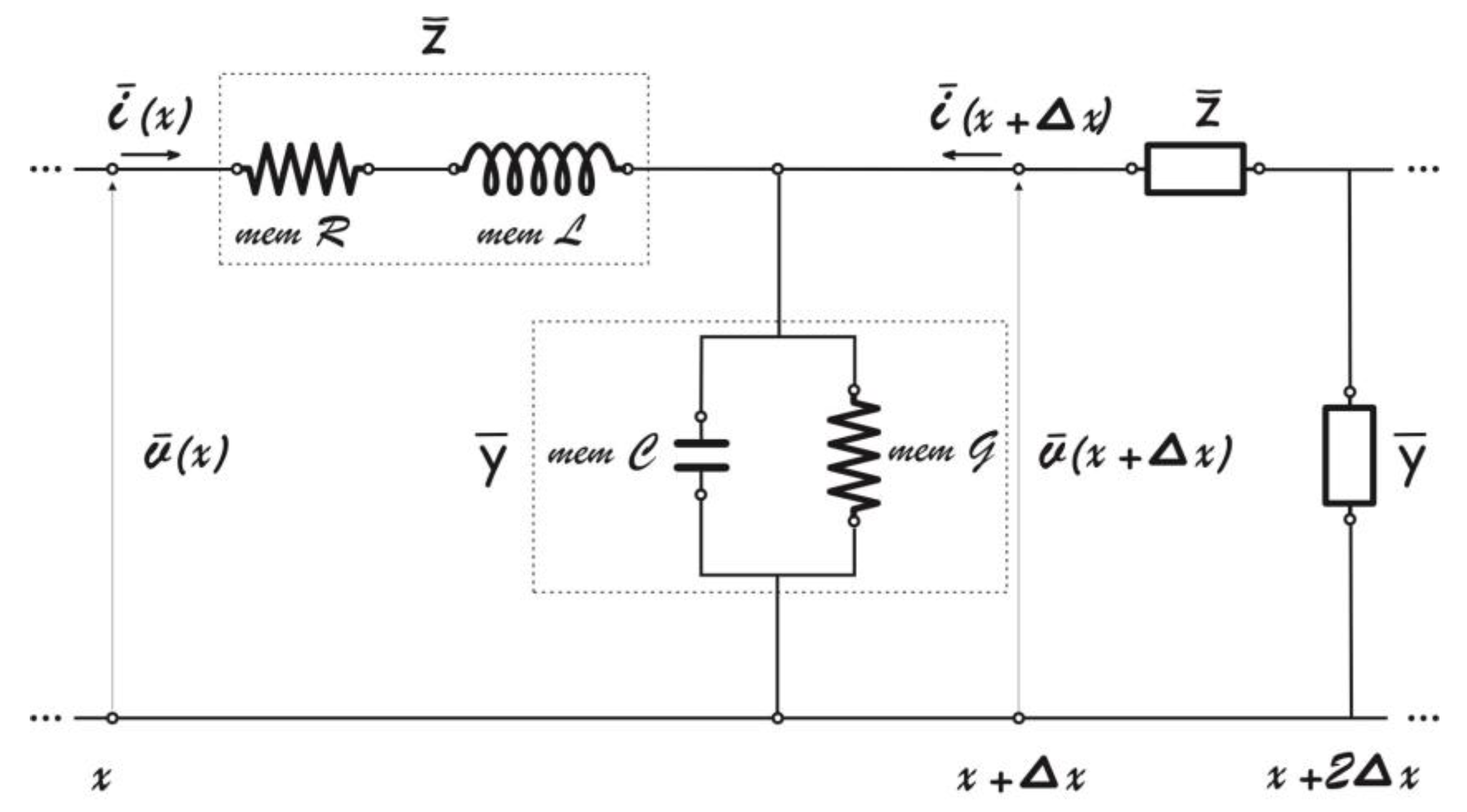
Figure 2.
Equivalent quadripoles used for calculating surface variations of temperature or heat flux. (a) Equivalent (symmetric two-port) network for temperature (T-network); (b) Equivalent (symmetric two-port) network for heat flux (П network). Symbol denotes the equivalent thermal impedance of the sample backing.
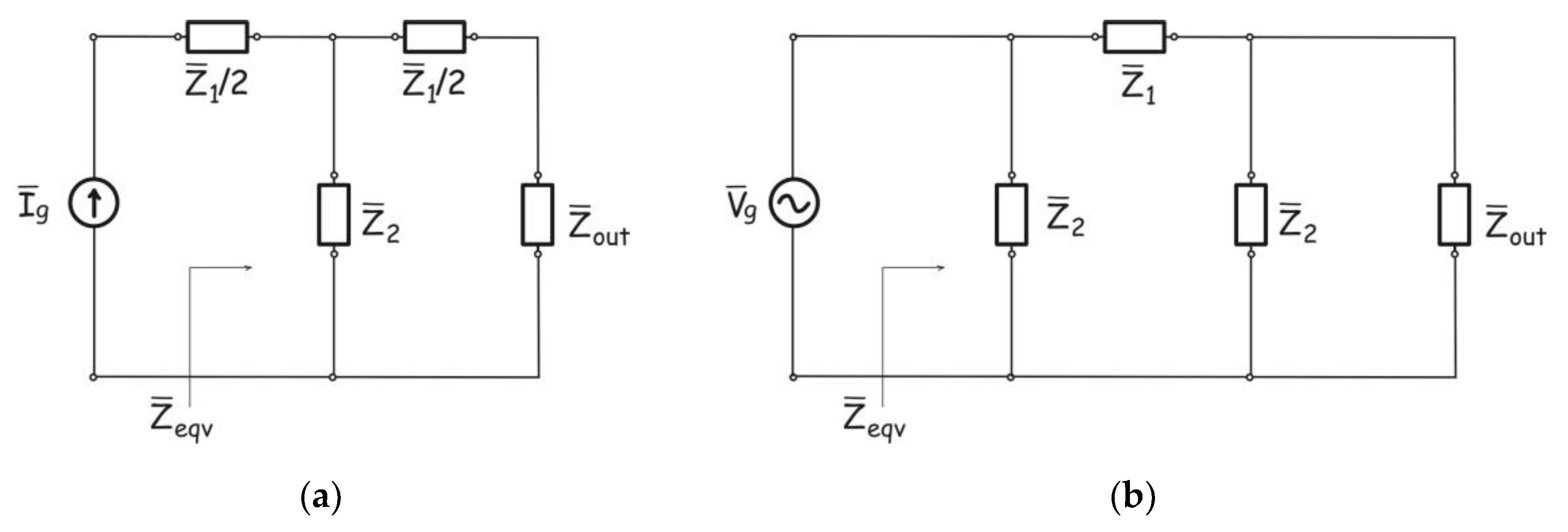
Figure 3.
Equivalent electrical scheme for calculating surface temperature variations in a semi-infinite sample.
Figure 3.
Equivalent electrical scheme for calculating surface temperature variations in a semi-infinite sample.
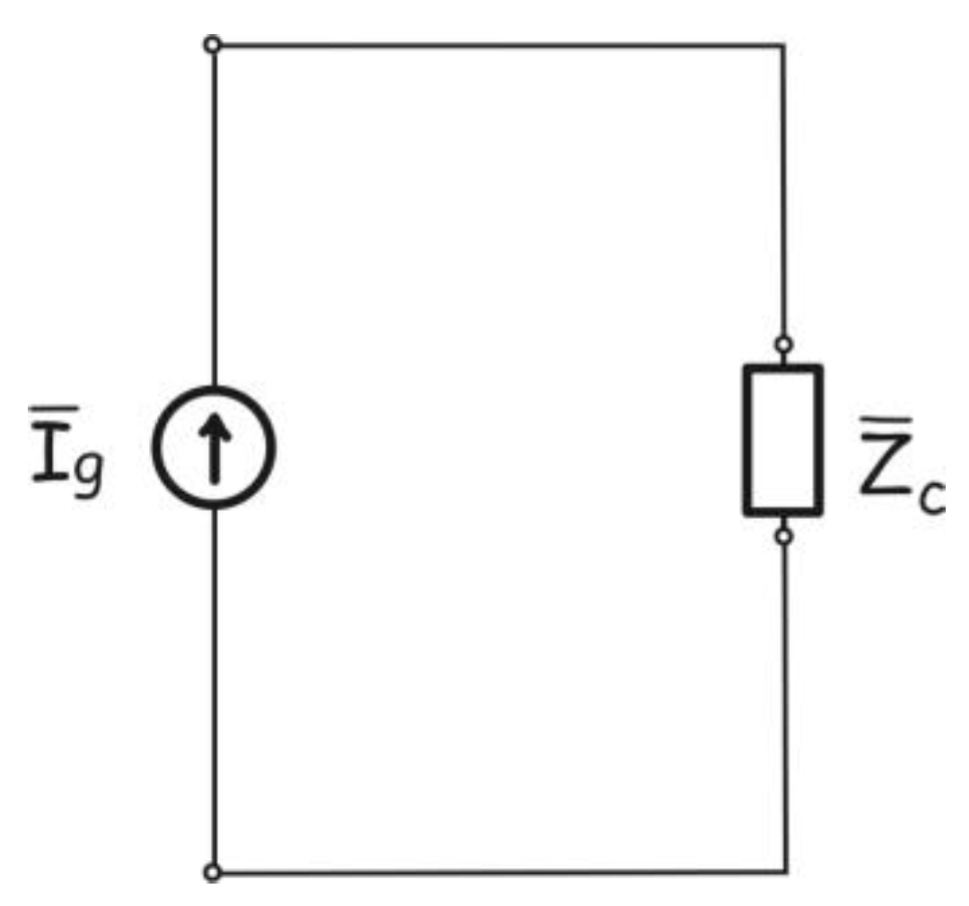

Table 1.
Systematic overview of properties of Caputo and ABC types of operators.
| Feature | Caputo operator | Atangana–Baleanu (ABC) operator | |
|---|---|---|---|
| Kernel type | Singular kernel with power-law decay (t−τ)−α | Non-singular kernel based on one parameter Mittag–Leffler function | |
| Memory structure | Long-tailed (slowly decaying) memory: strong influence of the distant past | Exponentially tempered memory: smooth fading of past influence | |
| Physical meaning | Suitable for systems with slow relaxation | Suitable for systems with multiple relaxation scales | |
| Initial conditions | Require classical initial conditions (integer-order derivatives), physically intuitive and practically applicable | Same treatment of initial conditions as Caputo, but extended to nonsingular memory kernels | |
| Spectral response | Pure power-law frequency response | Modified spectral response with exponential damping | |
| Examples of applications | Tansport of mass, energy or charge in glassy and polymeric systems, biological tissues, amorphous porous materials; | Transport in heterogeneous media with hierarchical structure; neural and cardiac tissue modeling | |
Table 2.
Systematic overview of kinetic and inertial memory effects, based on the electrical-analogy approach.
Table 2.
Systematic overview of kinetic and inertial memory effects, based on the electrical-analogy approach.
| Heat conduction theory | Thermal conductivity | Heat capacity | Microscopic picture | Energy (thermodynamical) effect |
| Classical parabolic (without memory) | Real, frequency- independent | Real, frequency- independent | Fast localized modes (molecular rotations, bond vibrations). Energy transported by short-lived collective modes (phonons, collective vibrations). | Energy stored in fast local modes; dissipation along the flux due to scattering of collective modes. |
| Debye relaxation (exponentially decaying kinetic memory) | Real, frequency independent | Real + imaginary, frequency-dependent, imaginary part vanishes at low frequencies. | Slow localized modes may be trapped in metastable states; energy transported by short-lived collective modes | Local accumulation in fast modes; additional dissipation within the local volume (imaginary part of complex heat capacity) feeding the entropic reservoir; dissipation along the flux due to scattering. |
| Fractional subdiffusive theory (kinetic memory via fractional operator kernel) | Real, frequency- independent | Real + imaginary, frequency dependent | Describes the full spectrum of localized modes, from those that relax at infinite speed to those with long-lived relaxation; Energy still transported by short-lived collective modes (phonons, collective vibrations). | Frequency-dependent accumulation and dissipation in the local volume; frequency independent dissipation along the flux due to scattering of collective modes |
| Hyperbolic/damped-wave theory (second sound, SPL; inertial memory via fading kernel) | Real + imaginary, frequency-dependent, imaginary part vanishes at low frequencies. | Real, frequency independent | Energy oscillates between fast localized modes and long-lived delocalized modes (phonons, collective vibrations); wave-like effects arise; no metastable trapping (all local modes infinitely fast). | Accumulation in local modes + additional accumulation in the flux; dissipation, if present, occurs only along the flux. |
| Fractional wave-like theory (inertial memory via fractional operator kernel) | Real + imaginary, frequency dependent | Real, frequency independent | Oscillations between fast localized and multiscale living delocalized modes; hierarchical energy oscillations. No metastable trapping. | Frequency-dependent accumulation in the flux, frequency independent accumulation in local volume; frequency dependent dissipation along the energy flux (short-lived and long lived collective modes) |
| Classical dual-phase-lag (DPL) theory | Real + imaginary, frequency-dependent, imaginary part vanishes at low frequencies. | Real + imaginary, frequency-dependent, imaginary part vanishes at low frequencies. | Combined influence of slow localized and long-lived collective modes. Wave-like effects may be damped or lost depending on collective mode lifetime and local mode relaxation time. | Accumulation in local modes and in the flux; dissipation both in the local volume and along the flux |
| Fractional DPL models | Real+ imaginary, frequency-dependent. | Real + imaginary, frequency-dependent | Influence of fast/slow localized modes and short-/long-lived collective modes. Wave-like effects at high frequency and subdiffusive effects at low frequencies. | Frequency dependent accumulation in local modes and in the flux; frequency dependent dissipation in the local volume and along the flux |
Disclaimer/Publisher’s Note: The statements, opinions and data contained in all publications are solely those of the individual author(s) and contributor(s) and not of MDPI and/or the editor(s). MDPI and/or the editor(s) disclaim responsibility for any injury to people or property resulting from any ideas, methods, instructions or products referred to in the content. |
© 2025 by the authors. Licensee MDPI, Basel, Switzerland. This article is an open access article distributed under the terms and conditions of the Creative Commons Attribution (CC BY) license (http://creativecommons.org/licenses/by/4.0/).
Copyright: This open access article is published under a Creative Commons CC BY 4.0 license, which permit the free download, distribution, and reuse, provided that the author and preprint are cited in any reuse.


