
Submitted:
21 September 2025
Posted:
22 September 2025
You are already at the latest version
Abstract
Debris flow erosion is key to the escalation of potential hazards, which may jeopardize the sustainable development of nearby human habitats. However, studies pertaining to this issue are impeded by the intricate interactions of flow and sediment. Thus, this study introduces an unresolved CFD-DEM coupled simulation primarily relying on a classical numerical simulation and a physical experiment to study critical erosion process of debris flows on a dry basal sediment under laboratory-scale.
Results indicate that three layers of substrate bed can be verified during the erosion process, and there is a positive correlation between the erosion depth and the particle size with the Froude number of debris flow, as well as between the erosion length and the critical entrainment transport with the total mass of debris flow. In addition, thresholds for the collisional point load and the impact energy of debris flow head, which are essential for predicting the attenuating rates of erosive depth and the critical entrainment transport, have been proposed based on data regressions derived from power functions.
The coupled numerical approach is capable of accurately simulating the erosion behavior of debris flows similarly to physical model experiments, thereby providing both theoretical and practical insights into the dynamics of erosion.
Keywords:
debris flow
; numerical simulation
; CFD-DEM
; critical erosion
1. Introduction
Debris flows are typically classified as multi-phase mass movements characterized by distinctive shear dynamics, diverse particle composition, as well as variations in runout distance and volume [1,2,3]. The erosion of debris flow refers to complex flow-sediment interaction mechanisms that induces varied eroding magnitude, mobilization, and deposition [4,5,6,7]. The erosion dimension from the initiation of the flow should be taken into consideration to study how this phenomenon emerges or ends, which is vital to early-warning system and counter-measures [8,9]. Various methods, including quasi-theoretical analysis, physical model experiment, field testing, and numerical simulation, have been employed to study erosion, with the erosion or entrainment rate serving as a key indicator for sediment transport models e.g. [5,6,10,11,12]. Egashira et al. [13] conducted experiments in a flume and discovered that the erosion rate of debris flows is closely related to the grain size of the eroding bed particles, and it has no significant correlation with the solid volume fraction of the debris flow. Berger et al. [10] indicated the commencing of the erosion resulting from the collision between the debris flow head and the substrate by field measurements. This point was likewise emphasized by Choi and Song [14] and Jiang et al. [9], who both further asserted that the collisional stress associated with particle movements of the flow head is responsible for the erosion process of unsaturated or dry bed sediment. Besides, shearing stress is also proven to be one of the important parameters for entrainment models [12,15]. And Ning et al. [16] added the shearing stress and the peak discharge of debris flow are crucial to the erosion process of not only the substrate but also the bank if any. There seems insufficient evidence to determine which of the two types of stress is more potent in the erosion process. Furthermore, the critical erosion process that governs the run out of debris flow is still unclear.
Indeed, the erosion is supposed to be derived from the collision between flow head and bed sediment or bank, which can be defined by the collisional stress [9], while factors that affect the commencing of collision-induced erosion needed further understanding. Additionally, when the debris flow reaches maturity, the erosion rate is directly proportional to the net basal shear stress produced by the ensuing flow, which contains a great proportion of liquid [6]. Consequently, the erosion model of a debris flow is expected to demonstrate an initiation through particle collisions, followed by sediment transportation that is influenced by friction shearing on basal sediment[14]. In this matter, point loads denoting the initial collisional effects may be key to the model for anticipating the erosion. Such a hypothesis was verified by previous studies e.g. [17] but requires continuous data to backup its effectiveness. Numerical simulation from the perspective of fine observation is an emerging important means. The two-way coupling of CFD (Computation Fluid Dynamics) and DEM (Discrete Element Method) is expected to be a powerful and efficient tool for the numerical investigation of multi-phase flows [18,19]. The basic logic of the CFD-DEM coupling model, including the interactions among particles, between particles and CFD cells, and between particles and walls, is introduced through continuous and discrete algorithms. Various configuration is established based on the logic to meet different requirements, in aspects such as the dynamic viscosity associated with the nonlinear rheology of debris flow [7], the adopted smooth grid approach to refine the transfer of coupling information [20], and the coarse coupling without resolution in consideration of computation efficiency [21,22].
In comparison to physical model experiments, the documentation of erosion quantities without deposition effects, particle collisions and shearing frictions in a two-way coupling simulation is more feasible, as physical models primarily rely on indirect measurements and continuum-flow and/or depth-integrated estimations [11,23].
To address these issues, this paper introduces a CFD-DEM coupling method validated by a simple simulation and a physical model test. Then the methodology is adopted to simulate the erosion caused by debris flows on a dry bed sediment and to examine its correlation with various related factors. Factors for evaluating the collisional and shearing effects on erosion depth and longitudinal eroding range are mainly introduced and physically discussed.
2. Materials and Methods
2.1. Coupling Logics
The coupled simulation is mainly focusing on interaction forces between spherical particles and fluid constrained in an impermeable and rigid facet geometries. And a dam breach approach herein is employed for the initiation of a debris flow and the flow propagation upon based on some criteria [7,22].
Above all, the CFD-DEM coupling in this study is unresolved, meaning the fluid cell size is larger than the maximal diameter of solid particles, for accurate resolution of the particle volume fraction and hydrodynamic forces on the fluid grid. This situation is also a trade-off made to achieve better computation efficiency. To comprehensively understand the CFD-DEM coupling model, it is necessary to go through the details about the continuous feature of fluid (including air and liquid), the discrete contacts among particles, and most importantly the interaction of fluid-particle media.
The CFD method is started with the continuity equation, considering both air and water fluids [18]:
where is the porosity of a CFD cell; is the equivalent density of the fluid defined by air and liquid; is the mean velocity of the fluid through the cell. According to the above discrete-cell approach the averaged Navier-Stokes equation is introduced to solve the dynamics of fluid:
where denotes fluid pressure; is the interaction force on the fluid per unit cell volume.
As for the DEM side, the motion of a particular particle i (involving translation and rotation) is mainly based on the Newton’s Second Law while the resultant force is derived from gravitational, particle-particle contact and particle-fluid interaction forces:
where and are the mass and the rotational moment of inertia of particle i, respectively. is the torque generated by other particles imposing rotation. Herein the Hertzian-Mindlin contact law is dominantly introduced to govern the inter-particle contact criteria in DEM and the force-deformation law, which won’t be repeated in this study due to its reliability [7,18]. denotes the contact force exerted by other particles. is the interaction force exerted from the fluid cell integrated with the drag force , buoyancy force , and lifting force . These forces are briefly introduced as follows:
where is the particle diameter, the particle velocity, and the correcting coefficient of porosity, representing the influence from other solid particles within the cell. And the is computed by:
where denotes the Reynolds number defined at the particle diameter scale, yielding:
where is the dynamic coefficient of viscosity. And is the drag coefficient which can be computed according to [24]:
The buoyancy force is defined by the affecting volume Vs and the gradient of the fluid pressure p:
Herein the lifting forces are introduced in the model in case the low solid fraction of debris flow.
where and are the relative linear and angular velocities between particles and fluid, respectively. denotes lifting coefficient and has the following expression :
During the development of the two-phase movement, the negative term of the sum of and is distributed back to the fluid cell, becoming .
At last, the MPI criteria (Message Passing Interface) is utilized to implement fluid and particle media kinematic information exchange including interaction force and particle movements. The frequency of the exchange is set to 10 time step in the CFD domain while it is one time step in the DEM.
The calibration of the model parameters is expected to be ensured following meticulous benchmarking procedures [18,25,26,27]. To do so, the CFD-DEM coupling herein is firstly benchmarked using a concise simulation plan involving a spherical particle (with a diameter of 1 mm) sinking in an initially static liquid under drag force, buoyancy force and gravity interpreted by the CFD domain. This approach was proven to be efficient in terms of quick benchmarking [28] and the coupling interaction governed by multiple parameters is then verified. The particle is descending in a 0.2*0.2*0.6 m CFD domain. The descending velocity of the particle in this design scenario served as the dominant factor for comparison with the one solved by the empirical analytical model [7,20]. The analytical varied with time computed according to [29], is added to compare with the numerical solution. As shown in Figure 1 the plotted data set of fits the analytical model rather well, justifying the interaction forces set in the coupling framework.
2.2. Experiments for Validation
Indeed, this simulation failed to fully capture the dynamic scenarios especially for the angular contacts and the porosity evolution among particles. Since the pore water pressure evolution is one of the essential indices that affect the debris-flow dynamics and transportation [12,30,31,32,33], we have added a series of physical flume model tests as prerequisite to further validate the numerical model of debris flow. The pore pressure dissipation within the flow propagation of both physical and numerical approaches was compared.
The flume which has the length and the width of 5.6 m and 0.3 m respectively is inclined by 20 degrees initially and the base-plate is paved without sediments serving as a rigid bed (Figure 2a). A mixture of sand gravel, clay and water with a solid fraction is mixed together to mimic real debris flows (76 % of grain, 24 % of water and clay), which has been already introduced by [34]. The mixture is firstly put and kept stirring in a hopper located at the top of the flume and then is released through the gate at the bottom of the hopper forming a moving slide on the rigid flume bottom. A pore pressure sensor is placed at the bottom plate 3 m downstream from the top trying to detect the pore pressure during the mature flow propagation and the sampling rate is 100 HZ. The right side of the flume is transparent, and a camera is employed to trace the flow process. On the other hand, the numerical model is established based on the physical flume model, except the distribution of the particle size was reduced to enhance computational efficiency, as specified in the Table 1. Based on the physical flume model, the whole motion during this numerical simulation is bounded by a box geometry (forming a chute inclined by 20 degrees) with 5.0 m length, 0.3 m width and 1.0 m height (Figure 2b). The debris flow mixture, referred to as a pack of DEM particles with a uniform diameter of 20 mm, is initially confined within a box filled with the CFD fluid at the upper section of the chute (0.3*0.5*0.5 m), and is subsequently initiated in accordance with a dam-breach pattern. In this context, we emphasize the significance of pore pressure dissipation in comparison to the one in the physical model test, thus the pore pressure evolution data set is directly computed by the detected water level within the debris flow head, which gives:
where h is the height from liquid surface to the bottom boundary. Note that the pore pressure here is considered as only the liquid flow propagation within debris flow and no excess pore pressure was taken into consideration due to the coarse grains-feature of the frontal head [35,36].
The numerical simulation trial here demonstrates close agreement with the physical model in terms of the maximum magnitude and the growth trend of the pore pressure, with both exhibiting a gradual dissipation process (Figure 2d). However, distinct temporal discrepancies are also observed: the numerical model sustains elevated pore water pressure for a longer duration (4.0 sec) compared to the physical model’s 0.4 sec (as recorded by the pore pressure transducer), which still showed a continuing downward trend. The discrepancies could be resulted from different particle diameter distribution and porosity between the numerical and physical models. General findings indicate that the uniform spherical particle-pack setting in the coupled approach effectively captures the pore pressure dissipation patterns and provides a reliable representation of debris flow transport mechanisms. Besides the ratio of pore pressure to normal pressure of debris flow indicating the liquefaction was also compared. The values of are 0.5 for the numerical simulation and 0.7 for the physical test, respectively (Table 2), which are both within the appropriate range according to [37].
Moreover, as shown in Table 2, the comparison of the fluid kinematics of the numerical simulation with the physical experimental data set reveals that both the averaged velocity U and the thickness of the debris flow head in the physical model are smaller, while the Froude number as computed by Eqn. 12 and the final deposit depth are both quite close. This substantiates that the numerical simulation is able to effectively solve the flow kinematics driven by inertial forces.
In conclusion, following the aforementioned verification, the adopted parameter values were determined and listed in the right-hand column of Table 1.
2.3. Procedure for Formal Simulation Experiments
The formal simulation experiments adhere to the key perspectives from the validation experimental procedure, as detailed in the Section 2.2, including for instance the inclined (fixed 20 degrees) chute defined by wall geometries, the dam breach-like initiation of debris flow, and the CFD resolution etc. A notable distinction from the validation experiment is that in formal experiments an additional pack of DEM spherical particles with uniform diameter of 10 mm served as a layer of dry bed sediment, 0.06 m thick, is paved across the bottom-bound geometry (Figure 3).
Mixtures comprising three types of masses, grain size distributions, and solid fractions, respectively, are generated to produce debris flows with diverse flow regime or dynamics along the x-axis in Figure 3b and interacting with a dry basal sediment. The detailed configuration of experimental variables is presented in Table 3, and the experimental serial nomenclature is established based on the conditions. It is noteworthy that uniform grain diameter distribution of the debris mixture as well as the basal sediment is setup in each case as a representative of the mean grain diameter of in-situ debris flow, and the given diameter of debris particles is always larger than that of the bed sediment with a diameter of 10 mm (see Table 1).
3. Results
In this section, the erosion process is analysed progressively in relation to bed sediment surface morphology and its mesoscopic interactions with the flows. Along the flow direction (x-axis in Figure 3), by measuring the volume variation of the erodible bed along the z-axis within each 0.01 m interval ( = 0.01 m) and dividing it by the base area, an averaged erosion depth is obtained. Accordingly, the dimension of the eroded material are quantified.
3.1. Erosion Phases
The initiation of the dam-break of the mixture signifies the time of 0 seconds. Even with differing experimental conditions, the erosion process can be generally divided into three phases: i) incipient intrusion into the substrate, namely the initial phase; ii) the net erosion phase; and iii) flowing attenuation leading to deposition, namely the post erosion phase. Sediment transport varied slightly depending on experimental conditions. In the following content, case D4M185V55 is selected as the representative example for illustrating the phases of erosion resulting from the most pronounced findings under high-dose of conditions, and the remaining cases are presented in the Appendix A.
In the initiation phase, the time duration varies slightly under different conditions, but is generally constrained within the range from 0 to 0.3 s. Debris mixture descends and flows forward, with a nearly uniform distribution of particle velocity (Figure 4a). It is believed that the descending is more pronounced, and the extent in erosion depth is negligible (less than 0.1 mm). The debris flow head develops at around x=0.6 m and ultimately reaches maximum x=1.8 m downstream. The generation is dependent on the dam-breach pattern while there are multiple different kinds of initiations in practice. Analysis relying on the particular initiating model does not hold significant practical guidance. Therefore, the phase serves solely as a temporal basis for distinguishing between the subsequent erosion and deposition phases.
During the net erosion phase, the primary concern is focusing on the spatial range where x > 0.6 m. The liquid profile in Figure 4b, similar to a surge wave, indicates the formation of the debris flow head, and the flow head moved along the x-axis from 1.2 to 3.1 m, with the associated time interval ranging from 0.3 to 3.2 s. The velocity of debris flow is stratified, typically increasing from the lower rear layer to the upper front (Figure 4b), indicating the highest erosion potential of the flow head. The effect of erosion on the bed sediment can be described as a plough induced by particle collisions. The particles located on the surface of the basal bed are characterized as being eroded at a velocity that approximates that of the flow head (Figure 4c). This shallow layer of particles is called the stimulated bouncing layer, and further down they are defined as shear-creeping layer and stationary layer, respectively, according to the velocity distribution (Figure 4c). The erosion rate herein (m/s) is determined according to the erosion depth measured along the y-axis at one certain position of x= m:
where and are the erosion depths at the time and , respectively. The erosion rate at x= m, as a function of time, exhibits a sharp increasing trend at the beginning, followed by a gentle decreasing trend toward the end of this phase (Figure 4d). As a result of the substantial collision between the debris flow and the surface particles, the particles from the eroded bed were incorporated into the initial erosion rate calculation (before time of 0.5 s). This led to a significantly large negative value for the erosion rate prior to reaching the peak value (Figure 4d). However, the subsequent curve can effectively represent the variation of the erosion rate over time. It can be deduced that the transient collision of particles contributes to the sharp increase in the erosion rate (at time of 0.6±0.1 s), allowing partial particles of the bed move at a velocity nearly identical to that of the debris flow and form like a surge front (Figure 4c). And the gentle decreasing erosion from 0.6±0.1 to 3.2±0.1 s, indicating the shear-creeping layer of the bed, results from the shearing friction afterwards. The two layers of the erodible bed will be further discussed later on.
On the other hand, the erosion rate fluctuates a little and tends to zero after 2.2 s (Figure 4d), indicating the onset of the attenuation phase. In a longitudinal perspective, there is a prevailing trend of thicker deposition observed in the rear segment, contrasted with thinner deposition in the front segment, while the flow body with the eroded materials extends to the farthest point of x = 4.63 m (Figure 5a). The erodible bed exhibits an arrow-like shape, with greater depth in the middle central region and shallower profiles at both lateral sides. This reveals that during the erosion process, the rheology of the debris flow still prevails, with a larger momentum in the centre and smaller momentum on the sides (Figure 5b). The particles of the bed upstream are evidently eroded, thereby leaving a shallow trench upstream while elevating the bed surface downstream (Figure 5c), and the demarcation line separating these two areas fluctuates between x=1.2 and x=1.8 m, depending on varying conditions (x=1.8 m in the case D4M185V55). It is noteworthy that the eroded interface of the bed material is presented as averaged values under unit width of the flume. Once again, we direct our attention to locations where the flow head has reached the net erosion state (x > 0.6 m) to eliminate any potential bias that may arise from the initiation of the dam breach. As shown in the red dotted oval in Figure 5c, the erosion quantities in that area is neglected.
3.2. Factors Contributing to Eroding Dynamics
In this context, the experimental variables, including the total mass, particle size, solid fraction of debris flows, and the derived kinematic parameters, were selected as factors to evaluate erosion. The analysis is mainly performed on the erosion depth at x = 1.2 - 1.4 m, where all the authorized debris flows transit into the net erosion phase and the flow heads shape up. According to Section 2.2 and Section 3.1, the Froude number is primarily employed to assess the flow dynamics. The longitudinal erosion range as well as the entrainment is further evaluated. All data results in relation to experimental variables can be checked in Table A1.
Figure 6 illustrates that the particle size D of the debris flow exhibits a strong positive correlation with the final erosion depth H (correlation coefficient r = 0.796), whereas the total mass M and the solid fraction V demonstrate weaker and the weakest correlations with H (r = 0.556 and 0.189), respectively. This trend is likewise observable in the relationship between the erosion length L and the aforementioned factors, whereas the correlation coefficient r between M and L is greater than that between M and H (0.895 compared with 0.556), and r between D and L is much smaller than that between D and H (0.219 compared with 0.796). Moreover, of the bed sediment, as indicated by the farthest approaching position of the post accumulation illustrated in Figure 5c, exhibits a stronger positive correlation with M, with r of 0.925. And the strongest positive correlation (r =0.938) between L and indicates that the large erosion magnitude could significantly enhance the run out of debris flow. Meanwhile, D and V show very limited correlation with L and .
It is also inferred from Figure 6 that a greater grain size D and mass M of debris flow, accompanied by a lower solid fraction V, may result in a larger , and the positive correlations between and H, L, and remain valid (showing r = 0.706, 0.549, and 0.526, respectively). Therefore, the grain size D and the mass M of debris flow are both explicitly key variables in the erosion process, with the exception of the V. And D has more evident impact on H while M has more evident impact on L and . In addition, the flow regime also has a considerable impact on the extent of the erosion. However, it is not reliable to directly compare the impacts of M and D on erosion with that of , as M and D here have only three variations while has 27 runs.
3.3. Mechanical Factors
To further study the critical mechanisms underlying erosion and propagation, contact forces with respect to the collisional effect between the flow head and the basal particles were detected. The detection is focused on the debris particles within the range x= m where the flow head approaches at the commencing of the net erosion phase (when the time is s). And the collisional force is computed as the scalar quantities of the contact forces exerted from the particles of the flow head per unit:
where , , and are the components in the x, y, and z directions of the contact force, respectively, and is the number of the particles of the flow head reaching the given region. The contact force here is documented using the numerical coupling method, which encompasses normal and tangential components, and is also referred to as point loads. In this matter, as increases, it also increases H in proportion, meanwhile a curve indicated by power-law was able to match the data points with the coefficient of determination being equal to 0.92 and p-value much less than 0.05 (Figure 7a), revealing a significant statistical relationship between the two variables. The power-law was predominantly applied because of the trend suggesting that H should equal zero when in the absence of force. The slope of the fitting curve exhibits a trend of transitioning from steep to gentle around a certain range ( = 2.5 to 4 N), suggesting that this is a threshold of change in the erosion rate.
On the other hand, an impact energy approximation of debris flow head is introduced as an integrated factor affecting the length of the erosion, which leads to:
Similarly, a power-law regression model effectively interprets the relationship between and the impact energy E, and the increasing rate of along E is slow after E reaches from 130 to 150 J (Figure 7b). Further validation may be needed through addition of data set within a smaller range of E (e.g. E < 200 J). Accordingly, the collisional force is key to the erosion depth extent H while the impact energy E governs the critical erosion length . There are specific thresholds in and E that distinguish between rapid and slow rates of increase for H and .
4. Discussion
4.1. Mechanisms of the Critical Erosion
This study particularly emphasizes on the net erosion process, specifically examining how the erosion develops under varied conditions. The erodible sediment presented was distinctively noted as comprising the layers of bouncing and creeping shear, which has the same feature of granular flow [39,40]. Note is made that the two-layer sediment is mobilized at an averaged velocity (denoted as erosion velocity ) that is up to 9.1% of the one U of the flow head. When considered aside with the creeping shear layer, the bouncing layer can be classified as an instance of entrainment, as indicated by its mean velocity [41] (refer to Table A1), which is approximately 90% of U. That is why the downward displacement of the entrained material is close to the run-out distance of the debris flow. Therefore, the entrainment in this context can be understood as being initiated by transit interplay between the granular head of the flow and the basal particles, which includes both collisions and rapid increase in basal friction [42]. Subsequently the mobility of the flow body is maintained by the shearing friction [10,12,17].
The increase in grain size D and Froude number enhances the erosion depth H linearly where the flow head interacts with the bed, justifying the granular-enrichment feature of the flow head [42] as well as the dependency of the two parameters on the collisional stress [14]. Besides, since the contact force which denotes the point load follows a power-law with H (Figure 7a) and was recorded concurrently with the onset of the net erosion (time of s), the potential of the collision is supposed to prompt the normal-oriented excavation of the substrate [10]. A preliminary threshold of that lies within the range of 2.5 to 4 N is proposed to define the erosion increasing from fast to slow with the increase in , which is different from the frictional and/or collisional stresses proposed by [6,9,35]. The point load offers a viable alternative for assessing the erosion caused by debris flow, and our subsequent study will concentrate on the practical computation of .
The total mass M of the mixture being known as the magnitude or volume of debris flow has a positive effect on both the eroded length L and the critical entrainment migration . This can be elucidated by stating that an increase in mass leads to a reduction in internal friction [42], thereby enhancing mobility. Accordingly, the energy-oriented factor E that integrates M and (Eqn. 15) should be likely related to the critical eroding effects, and its regressive power-law relationship with confirms the idea. Since the computation of E indicates averaged flow depth h along the whole flow body, the trend highlights the significance of friction in the eroding dynamics [12,17]. Again, there is a preliminary threshold of E (within the range from 130 to 150 J) in controlling the rate of increase of L from fast to slow according to Figure 7b, and E is more feasible to obtain in fields than . In total, the critical erosion mechanism can be interpreted through a synthesis of both force-based and energy-based perspectives.
4.2. Limitations of this Study
This paper is focusing on the erosion of debris flow head on a dry bed sediment under laboratory-scale, thus the effect should be discussed if transferring to large-scale events. Now that several dimensionless numbers such as Froude number , Savage number , Bagnld number , and Friction number et al. have been demonstrated valid in debris-flow dynamics [36,43], our study chooses to preliminarily meet the similitude, meaning the Froude number of the model equals that of the prototype , expressed as follows: In the case where the geometric dimension ratio is set at 1 (model) to N (prototype), and where the density and the gravity acceleration g are both equal, the scale ratios for both force and energy here are established as 1 to .
For further exploration, angular particles and boundary conditions [44] on how the flow dynamics evolving more accurately are warranted. Indeed, intervals of the given variables need to be more refined [43] and flow attenuation affecting the energy estimation due to collisions or frictions should be added [45], in order to broaden the scope of the research.
5. Conclusions
Our study generally ascertains that the CFD-DEM coupled numerical simulations can effectively serve as an auxiliary or supplementary tool to physical model experiments, providing comprehensive feedback on the phenomenon of debris flow erosion, thus offering technical support for practical engineering or theoretical studies. The main results are listed as follows:
The process of erosion can be categorized into three distinct phases: the initial erosion phase, the net erosion phase, and the post-erosion phase, wherein the net erosion phase is responsible for the most significant erosive effects.Increasing both the grain size D and the Froude number of debris flow can enhance the erosion depth normal to the bed, and the eroded length L and the critical transport of the basal sediment are both positively correlated with the total mass M of the debris flow.
The erosion depth H is described by a power function that correlates with the collisional point load computed by the normal impact force per unit of the debris-flow head. Furthermore, the critical entrainment transport is also represented as a power function of the impact energy E estimated by the averaged thickness of the debris flow head.
Furthermore, thresholds for both the collisional point load and the impact energy that predict the attenuated rates of the erosive depth and the critical transport of entrainment, respectively, are obtained through regression analyses.
The idea for the mechanisms of the erosion proposed by previous studies is verified by the presented coupled simulation that the collisional point load is key to initiating the net erosion process, while frictional shearing is the factor that sustains the flow mobility.
Author Contributions
Conceptualization, H.M. and X.S.; methodology, H.M.; software, J.C. and R.D.; validation, H.M., L.J. and X.S.; formal analysis, H.M. and R.D.; data curation, Y.P.; writing—original draft preparation, H.M.; writing—review and editing, H.M. and L.J.; visualization, H.M. and X.S.; supervision, H.M. and X.S.; project administration, H.M., Z.L. and X.S.; funding acquisition, H.M. and Z.L.. All authors have read and agreed to the published version of the manuscript.
Funding
This research was funded by Natural Science Foundation of Sichuan Province grant number 2022NSFSC1123 and Sichuan Provincial Social Science Fund grant number SCJJ25RKX007
Data Availability Statement
The datasets generated and analysed during the current study are not publicly available due [RESEARCH UNIT POLICY] but are available from the corresponding author on reasonable request.
Acknowledgments
The numerical study is conducted using an open source parallel coupled CFD-DEM framework combining the strengths of LIGGGHTS® DEM code and the Open Source CFD package OpenFOAM®(*).
Conflicts of Interest
The authors declare no conflicts of interest.
Abbreviations
The following abbreviations are used in this manuscript:
| D | Uniform grain size of debris flow |
| M | Total mass of debris flow |
| V | Solid fraction of debris flow |
| H | Erosion depth |
| L | Erosion length |
| Critical entrainment transport | |
| Froude number | |
| U | Velocity of the debris flow head |
| Velocity of the eroded material | |
| Velocity of the entrainment | |
| h | Thickness of debris flow |
| g | Gravity acceleration |
| Collisional point load | |
| E | Impact energy of debris flow |
Appendix A Appendix for main results

Table A1.
Main results from the numerical simulation.
| Serial ID. | H (m) | L (m) | (m) | U (m/s) | (m/s) | h (m) | |
|---|---|---|---|---|---|---|---|
| ]1*D4M115V45 | 2.85 | 0.035 | 1.62 | 3.32 | 2.46 | 0.09 | 0.040 |
| ]1*D4M115V50 | 2.52 | 0.037 | 1.66 | 3.5 | 2.54 | 0.12 | 0.060 |
| ]1*D4M115V55 | 2.16 | 0.037 | 1.61 | 3.62 | 2.30 | 0.13 | 0.076 |
| ]1*D4M150V45 | 4.04 | 0.037 | 1.75 | 4.05 | 2.37 | 0.15 | 0.034 |
| ]1*D4M150V50 | 2.86 | 0.038 | 1.85 | 4.13 | 2.54 | 0.18 | 0.060 |
| ]1*D4M150V55 | 2.82 | 0.039 | 1.92 | 4.40 | 2.46 | 0.20 | 0.071 |
| ]1*D4M185V45 | 3.86 | 0.039 | 1.94 | 4.45 | 2.46 | 0.20 | 0.044 |
| ]1*D4M185V50 | 3.14 | 0.040 | 1.94 | 4.56 | 2.51 | 0.23 | 0.070 |
| ]1*D4M185V55 | 2.74 | 0.040 | 2.10 | 4.63 | 2.59 | 0.24 | 0.095 |
| ]1*D3M115V45 | 1.65 | 0.031 | 1.47 | 3.32 | 2.15 | 0.08 | 0.113 |
| ]1*D3M115V50 | 2.03 | 0.033 | 1.57 | 3.35 | 2.08 | 0.10 | 0.077 |
| ]1*D3M115V55 | 1.97 | 0.033 | 1.63 | 3.63 | 2.24 | 0.11 | 0.083 |
| ]1*D3M150V45 | 2.25 | 0.035 | 1.83 | 3.92 | 2.13 | 0.13 | 0.097 |
| ]1*D3M150V50 | 2.47 | 0.034 | 1.67 | 4.00 | 2.18 | 0.13 | 0.085 |
| ]1*D3M150V55 | 2.33 | 0.037 | 1.80 | 4.28 | 2.21 | 0.17 | 0.098 |
| ]1*D3M185V45 | 2.92 | 0.036 | 1.89 | 4.34 | 2.26 | 0.17 | 0.071 |
| ]1*D3M185V50 | 2.75 | 0.037 | 2.02 | 4.36 | 2.13 | 0.18 | 0.092 |
| ]1*D3M185V55 | 2.36 | 0.038 | 1.94 | 4.58 | 2.28 | 0.18 | 0.118 |
| ]1*D2M115V45 | 1.65 | 0.028 | 1.46 | 3.13 | 1.65 | 0.07 | 0.109 |
| ]1*D2M115V50 | 1.87 | 0.028 | 1.56 | 3.30 | 1.71 | 0.08 | 0.091 |
| ]1*D2M115V55 | 1.73 | 0.030 | 1.62 | 3.64 | 1.72 | 0.10 | 0.108 |
| ]1*D2M150V45 | 2.19 | 0.031 | 1.65 | 3.79 | 1.68 | 0.11 | 0.105 |
| ]1*D2M150V50 | 2.12 | 0.031 | 1.76 | 3.94 | 1.70 | 0.13 | 0.105 |
| ]1*D2M150V55 | 2.17 | 0.033 | 1.85 | 4.10 | 1.72 | 0.14 | 0.116 |
| ]1*D2M185V45 | 2.45 | 0.033 | 1.95 | 4.27 | 1.73 | 0.14 | 0.109 |
| ]1*D2M185V50 | 2.89 | 0.034 | 1.86 | 4.30 | 1.87 | 0.15 | 0.084 |
| ]1*D2M185V55 | 1.93 | 0.034 | 1.87 | 4.53 | 1.81 | 0.16 | 0.154 |
References
- Berti, M.; Genevois, R.; LaHusen, R.; Simoni, A.; Tecca, P.R. Debris flow monitoring in the acquabona watershed on the Dolomites (Italian alps). Physics and Chemistry of the Earth, Part B: Hydrology, Oceans and Atmosphere 2000, 25, 707–715. [Google Scholar] [CrossRef]
- Yang, Z.Q.; Zhao, X.G.; Chen, M.; Zhang, J.; Yang, Y.; Chen, W.T.; Bai, X.F.; Wang, M.M.; Wu, Q. Characteristics, dynamic analyses and hazard assessment of Debris flows in Niumiangou valley of Wenchuan County. Appl Sci 2023, 13, 1161. [Google Scholar] [CrossRef]
- Li, C.J.; Hu, Y.X.; Li, H.B.; Zhou, J.W. Deciphering the dynamics of debris flows through basal stress responses in model experiments. Acta Geotechnica 2025, 20, 1777–1794. [Google Scholar] [CrossRef]
- Hungr, O.; McDougall, S.; Bovis, M. Entrainment of material by debris flows. In Debris-flow Hazards and Related Phenomena; Springer: Berlin, Heidelberg, 2005. [Google Scholar]
- Li, J.; Cao, Z.X.; Hu, K.H.; Pender, G.; Liu, Q.Q. A depth-averaged two-phase model for debris flows over fixed beds. International Journal of Sediment Research 2018, 4, 462–477. [Google Scholar] [CrossRef]
- Shen, P.; Zhang, L.M.; Wong, H.F.; Peng, D.L.; Zhou, S.Y.; Zhang, S.; Chen, C. Debris flow enlargement from entrainment: A case study for comparison of three entrainment models. Engineering Geology 2020, 270, 105581. [Google Scholar] [CrossRef]
- Wang, Y.H.; Mao, W.W.; Yang, P.; Huang, Y.; Zheng, H. CFD-DEM study on the entrainment induced by debris flows with the HBP rheological model. IOP Conf. Series: Earth and Environmental Science 2021, 861, 072012. [Google Scholar] [CrossRef]
- Stoffel, M.; Mendlik, T.; Schneuwly-Bollschweiler, M.; Gobiet, A. Possible impacts of climate change on debris-flow activity in the Swiss Alps. Climatic Change 2014, 122, 141–155. [Google Scholar] [CrossRef]
- Jiang, Y.; Song, P.; Choi, C.E.; Choo, J. Erosion and transport of dry soil bed by collisional granular flow: Insights from a combined experimental– numerical investigation. Journal of Geophysical Research: Earth Surface 2023, 128, e2023JF007073. [Google Scholar] [CrossRef]
- Berger, C.; Mcardell, B.W.; Schlunegger, F. Direct measurement of channel erosion by debris flows, Illgraben, Switzerland. Journal of Geophysical Research-Earth Surface 2011, 116. [Google Scholar] [CrossRef]
- Iverson, R.M.; Reid, M.E.; Logan, M.; LaHusen, R.G.; Godt, J.W.; Griswold, J.P. Positive feedback and momentum growth during debris-flow entrainment of wet bed sediment. Nat. Geosci. 2011, 4, 116–121. [Google Scholar] [CrossRef]
- Iverson, R.M. Elementary theory of bed-sediment entrainment by debris flows and avalanches. Journal of Geophysical Research: Earth Surface 2012, 117, F03006. [Google Scholar] [CrossRef]
- Egashira, S.; Honda, N.; Itoh, T. Experimental study on the entrainment of bed material into debris flow. Physics and Chemistry of the Earth, Part C: Solar, Terrestrial and Planetary Science 2001, 26, 645–650. [Google Scholar] [CrossRef]
- Choi, C.E.; Song, P. New unsaturated erosion model for landslide: Effects of flow particle size and debunking the importance of frictional stress. Engineering Geology 2023, 315, 107024. [Google Scholar] [CrossRef]
- Zheng, H.; Hu, X.; Shi, Z.; McArdell, B.; de Haas, T. Volumetric growth of debris flow on erodible bed by basal shear and collision: Theory and observations. Earth and Planetary Science Letters 2025, 662, 119404. [Google Scholar] [CrossRef]
- Ning, L.; Hu, K.; Li, P.; Cheng, H.; Liu, S.; Zhang, Q. Peak discharge amplication of debris flows in colluvial channels with varying cross-sections. Environmental Earth Sciences 2025, 84, 217. [Google Scholar] [CrossRef]
- Mcdougall, S.; Hungr, O. Dynamic modelling of entrainment in rapid landslides. Canadian Geotechnical Journal 2005, 5, 1437–1448. [Google Scholar] [CrossRef]
- Zhao, J.; Shan, T. Coupled CFD-DEM simulation of fluid-particle interaction in geomechanics. Powder Technol. 2013, 239, 248–258. [Google Scholar] [CrossRef]
- Kong, Y.; Zhao, J.D.; Li, X.Y. Coupled CFD-DEM simulation of fluid-particle interaction in geomechanics. Proceedings of the Second JTC1 Workshop, Hongkong, China, October 2018.
- Razavi, F.; Komrakova, A.; Lange, C.F. CFD–DEM Simulation of Sand-Retention Mechanisms in Slurry Flow. Energies 2021, 14, 3797. [Google Scholar] [CrossRef]
- Kong, Y.; Li, X.; Zhao, J. Quantifying the transition of impact mechanisms of geophysical flows against flexible barrier. Engineering Geology 2021, 289, 106188. [Google Scholar] [CrossRef]
- Kong, Y.; Li, X.; Zhao, J.; Guan, M. Load–deflection of flexible ring-net barrier in resisting debris flows. Géotechnique 2022, 74, 486–498. [Google Scholar] [CrossRef]
- Han, Z.; Chen, G.; Li, Y.; Tang, C.; Xu, L.; He, Y.; Huang, X.; Wang, W. Numerical simulation of debris-flow behavior incorporating a dynamic method for estimating the entrainment. Engineering Geology 2015, 190, 52–64. [Google Scholar] [CrossRef]
- Schiller, L.A.; Nauman, A. A drag coefficient correlation. Z. Vereines Ingenieure 1935, 77, 318–320. [Google Scholar]
- Li, X.; Zhao, J. Dam-break of mixtures consisting of non-Newtonian liquids and granular particles. Powder Technol. 2018, 338, 493–505. [Google Scholar] [CrossRef]
- Li, X.; Zhao, J.; Kwan, J.S.H. Assessing debris flow impact on flexible ring net barrier: A coupled CFD-DEM study. Computers and Geotechnics 2020, 128, 103850. [Google Scholar] [CrossRef]
- Li, X.; Zhao, J.; Soga, K. A new physically based impact model for debris flow. Géotechnique 2021, 71, 674–685. [Google Scholar] [CrossRef]
- Zhao, T.X.; Li, X. Numerical Investigation on Sediment Bed Erosion Based on CFD-DEM. In: In: Zhang, JM., Zhang, L., Wang, R. (eds) Dam Breach Modelling and Risk Disposal. ICED 2020. Springer Series in Geomechanics and Geoengineering, Springer: Cham., 2020.
- Levenspiel, O.; Haider, A. Drag Coefficient and Terminal Velocity of Spherical and Nonspherical Particles. Powder Technol. 1989, 58, 63–70. [Google Scholar] [CrossRef]
- George, D.; Iverson, R.M. A two-phase debris-flow model that includes coupled evolution of volume fractions, granular dilatancy, and pore-fluid pressure. Italian Journal of Engineering Geology and Environment 2011, 415–424. [Google Scholar]
- Liu, W.; He, S.; Li, X. A finite volume method for two-phase debris flow simulation that accounts for the pore-fluid pressure evolution. Environmental Earth Sciences 2016, 75, 206. [Google Scholar] [CrossRef]
- Iverson, R.M.; Denlinger, R.P. Flow of variably fluidized granular masses across three-dimensional terrain: 1 Coulomb mixture theory. Journal of Geophysical Research 1989, 58, 537–552. [Google Scholar] [CrossRef]
- Tayyebi, S.M.; Pisano, M.; Stickle, M.M. Two-phase SPH numerical study of pore-water pressure effect on debris flows mobility: Yu Tung debris flow. Computers and Geotechnics 2021, 132, 103973. [Google Scholar] [CrossRef]
- Huo, M.; Lambert, S.; Fontaine, F.; Piton, G. Capture of near-critical debris flows by flexible barriers: an experimental investigation. Natural Hazards and Earth System Sciences submitted. 2025. [Google Scholar]
- Song, P.J.; Choi, E.C. Revealing the importance of capillary and collisional stresses on soil bed erosion induced by debris flows. Journal of Geophysical Research: Earth Surface 2021, 126, 1–16. [Google Scholar] [CrossRef]
- Iverson, R.M. The physics of debris flows. Reviews of Geophysics 1997, 3, 245–296. [Google Scholar] [CrossRef]
- Ouyang, C.; He, S.; Tang, C. Numerical analysis of dynamics of debris flow over erodible beds in Wenchuan earthquake-induced area. Engineering Geology 2015, 194, 62–72. [Google Scholar] [CrossRef]
- Bagnold, R.A. Experiments on a gravity-free dispersion of large solid spheres in a Newtonian fluid under shear. Proceedings of the Royal Society of London. Series A. Mathematical and Physical Sciences 1954, 225(1160), 49–63. [Google Scholar] [CrossRef]
- Sarno, L.; Carleo, L.; Papa, M.N.; Villani, P. Experimental investigation on the effects of the fixed boundaries in channelized dry granular flows. Rock Mechanics and Rock Engineering 2018, 51, 203–225. [Google Scholar] [CrossRef]
- Komatsu, T.; Inagaki, S.; Nakagawa, N.; Nasuno, S. Creep motion in a granular pile exhibiting steady surface flow. Physical Review Letters 2001, 9, 1757–1760. [Google Scholar] [CrossRef]
- Pudasaini, S.P.; Krautblatter, M. The mechanics of landslide mobility with erosion. Nature communications 2021, 12, 6793. [Google Scholar] [CrossRef]
- Liu, H.W.; Zhao, X.Y.; Frattini, P.; Crosta, G.B.; De Blasio, F.V.; Wan, Y.H.; Zhu, X.Z. Mobility and erosion of granular flows travelling on an erodible substrate: Insights from the small-scale flume experiments. Engineering Geology 2023, 326, 107316. [Google Scholar] [CrossRef]
- Pandey, N.K.; Satyam, N. Entrainment-driven morphological changes in debris flow deposits by varying water content at laboratory scale. Bulletin of Engineering Geology and the Environment 2025, 84, 215. [Google Scholar] [CrossRef]
- Iverson, R.M. Scaling and design of landslide and debris-flow experiments. Geomorphology 2015, 244, 9–20. [Google Scholar] [CrossRef]
- Federico, F.; Cesali, C. An energy-based approach to predict debris flow mobility and analyze empirical relationships. Canadian Geotechnical Journal 2015, 12, 2113–2133. [Google Scholar] [CrossRef]
Figure 1.
(left) the data set of the velocity of the sinking particle varied with time from analytical model and numerical calculation and (right) the simulation scene.
Figure 1.
(left) the data set of the velocity of the sinking particle varied with time from analytical model and numerical calculation and (right) the simulation scene.
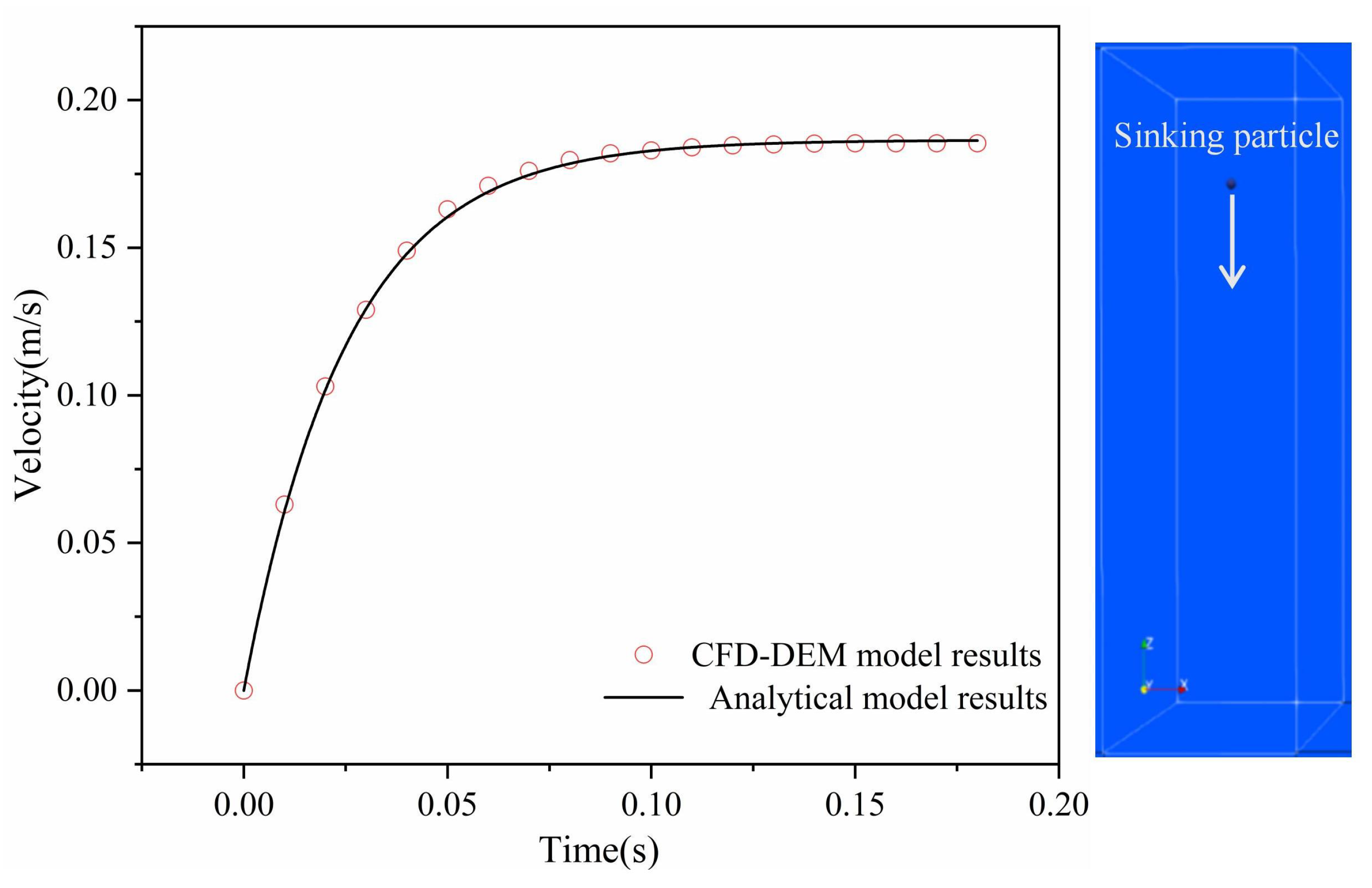
Figure 2.
comparative analysis of pore pressure evolution presented between (a) the physical flume model and (b) the numerical model (60*60 mm per grid), as well as (c) the flow profile in the real model (50*50 mm per grid) and (d) the data set obtained from the numerical computation and the actual sensor.
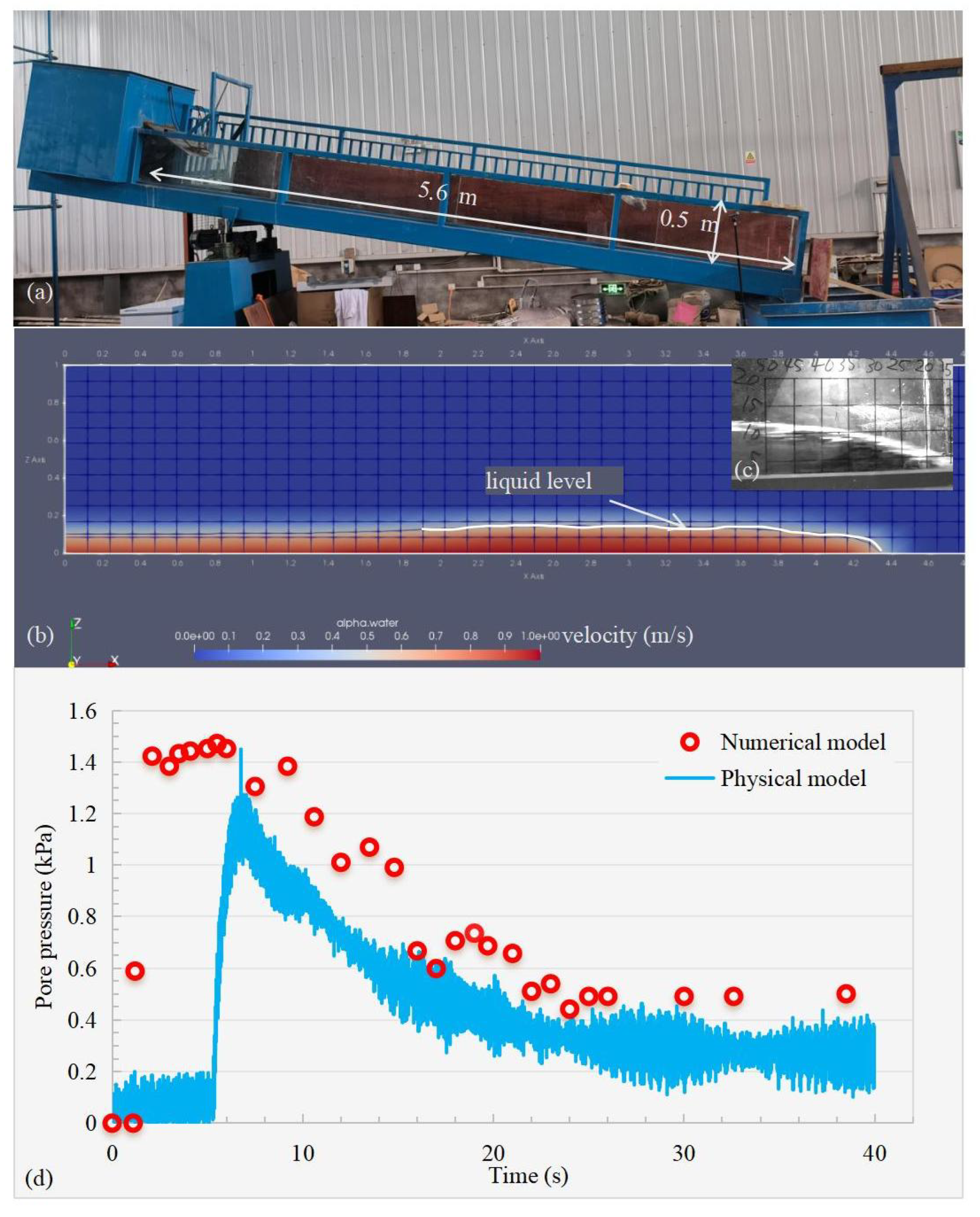
Figure 3.
Numerical simulation setup of (a) the axonometric view, (b) the longitudinal view ( inside means inclined angle of 20 degrees), and (c) the frontal view of the model.
Figure 3.
Numerical simulation setup of (a) the axonometric view, (b) the longitudinal view ( inside means inclined angle of 20 degrees), and (c) the frontal view of the model.
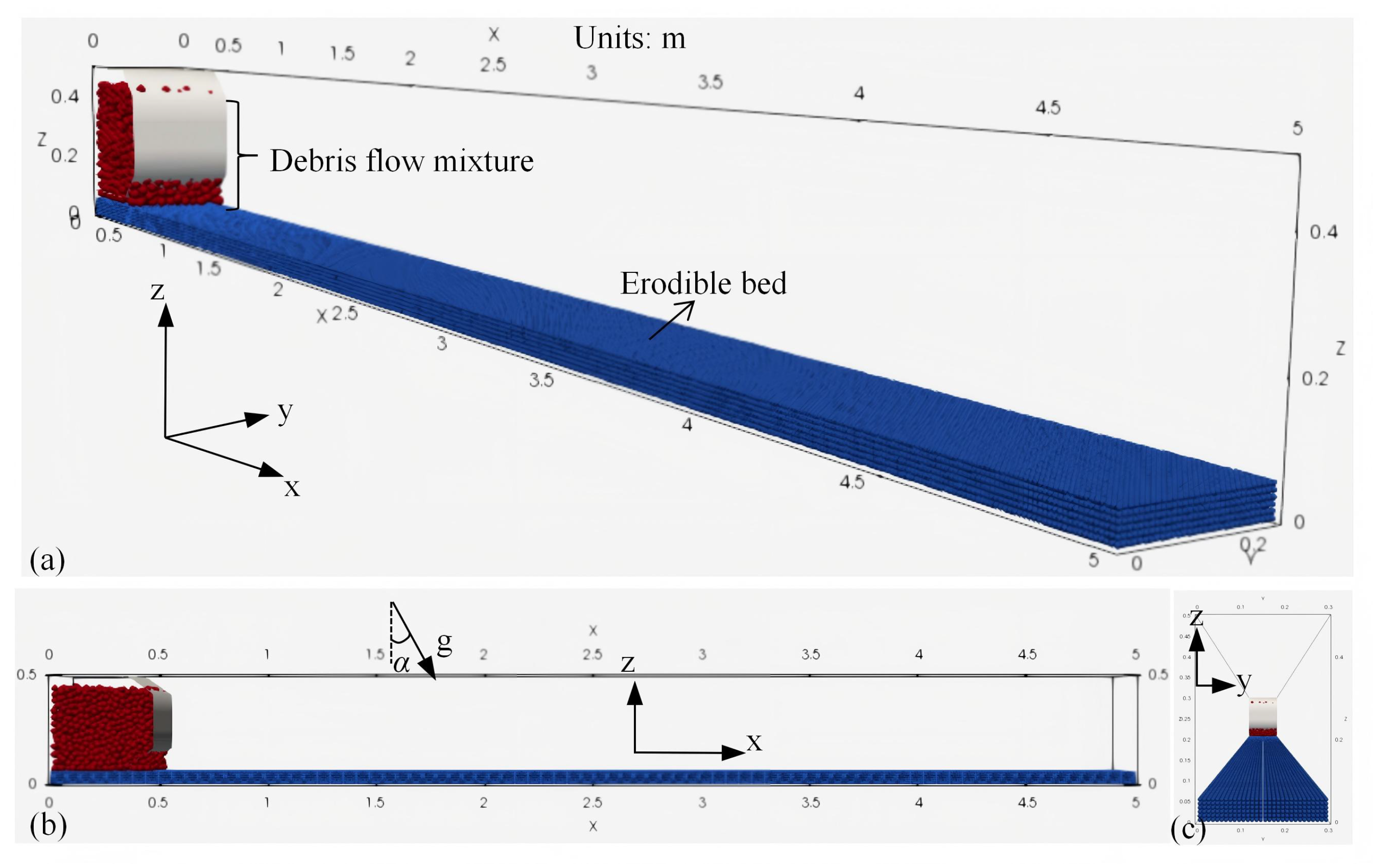
Figure 4.
The erosion processes (taking D4M185V55 as an example): (a) initial phase, (b) the debris flow propagation and (c) the separated erodible bed at the net erosion phase, and (d) the erosion rate varying with time.
Figure 4.
The erosion processes (taking D4M185V55 as an example): (a) initial phase, (b) the debris flow propagation and (c) the separated erodible bed at the net erosion phase, and (d) the erosion rate varying with time.
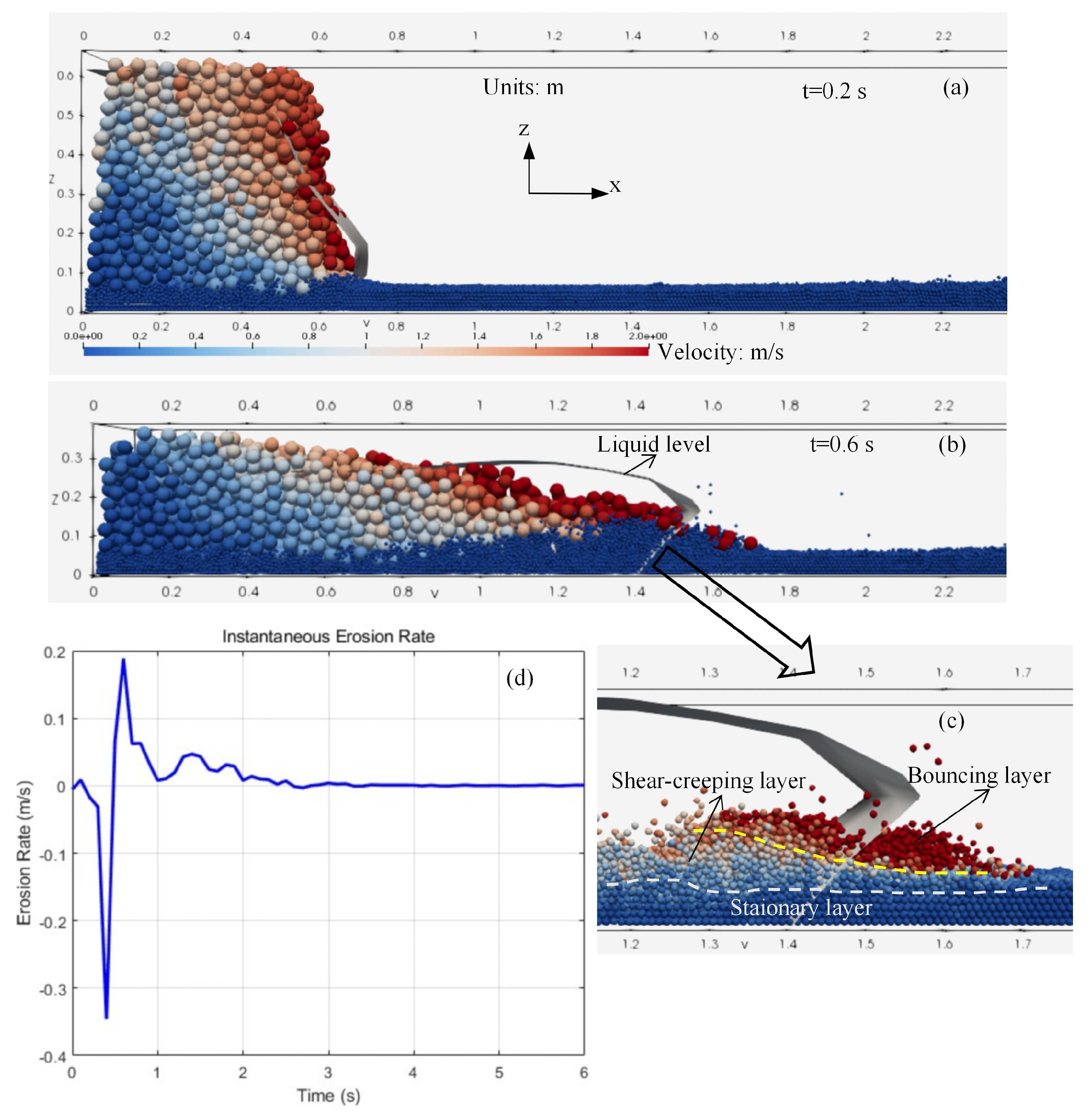
Figure 5.
The post erosion phase (taking D4M185V55 as an example): (a) the longitudinal view, (b) the plan view, and (c) the profile of the bed after erosion (note that H, L, and denote the erosion depth, the erosion length, and the critical bed sediment transport displacement, respectively).
Figure 5.
The post erosion phase (taking D4M185V55 as an example): (a) the longitudinal view, (b) the plan view, and (c) the profile of the bed after erosion (note that H, L, and denote the erosion depth, the erosion length, and the critical bed sediment transport displacement, respectively).
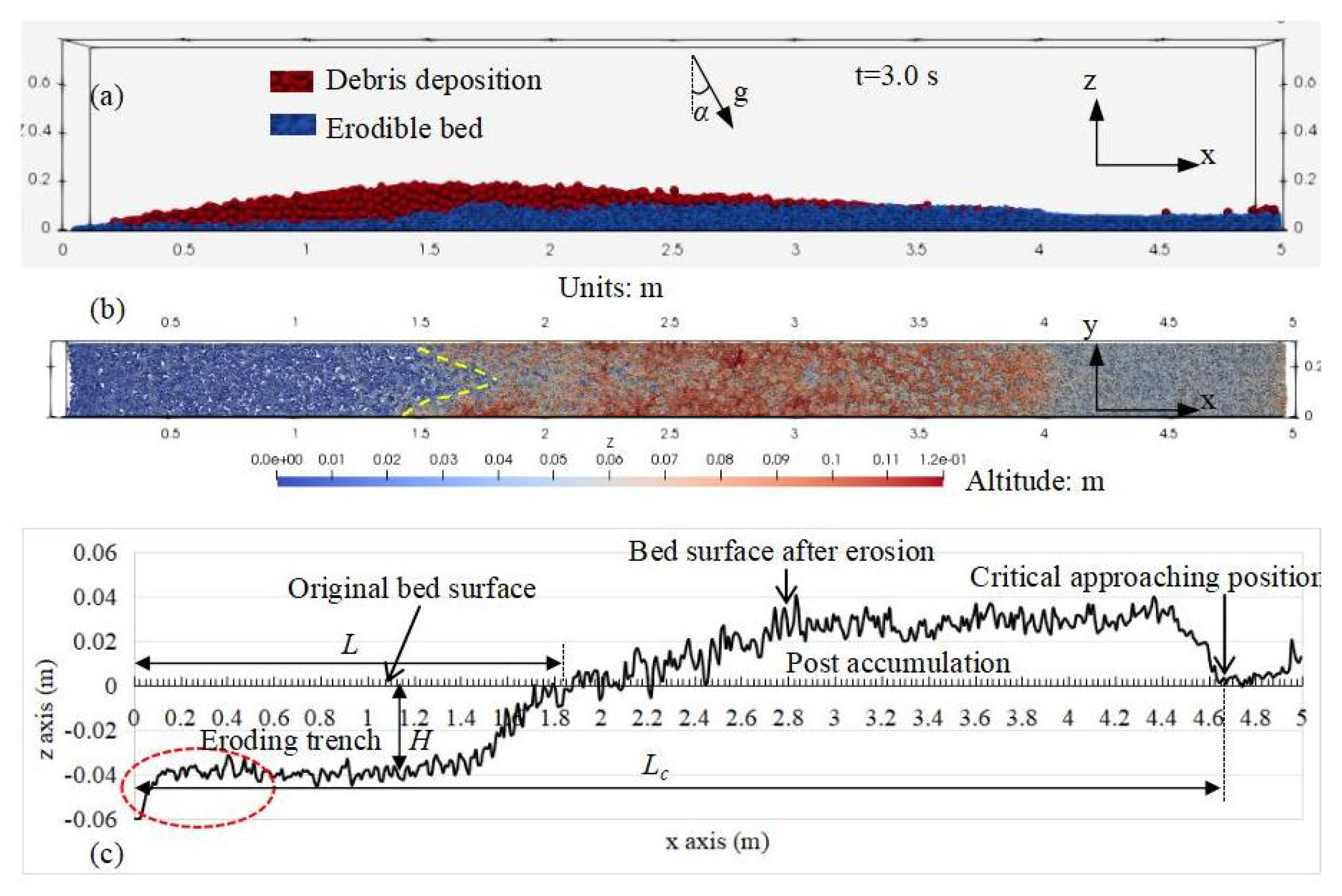
Figure 6.
The correlation pairs between the variables including , diameter D, total mass M, solid fraction V, the erosion depth H, the erosion length L, and the critical bed sediment transport displacement .
Figure 6.
The correlation pairs between the variables including , diameter D, total mass M, solid fraction V, the erosion depth H, the erosion length L, and the critical bed sediment transport displacement .
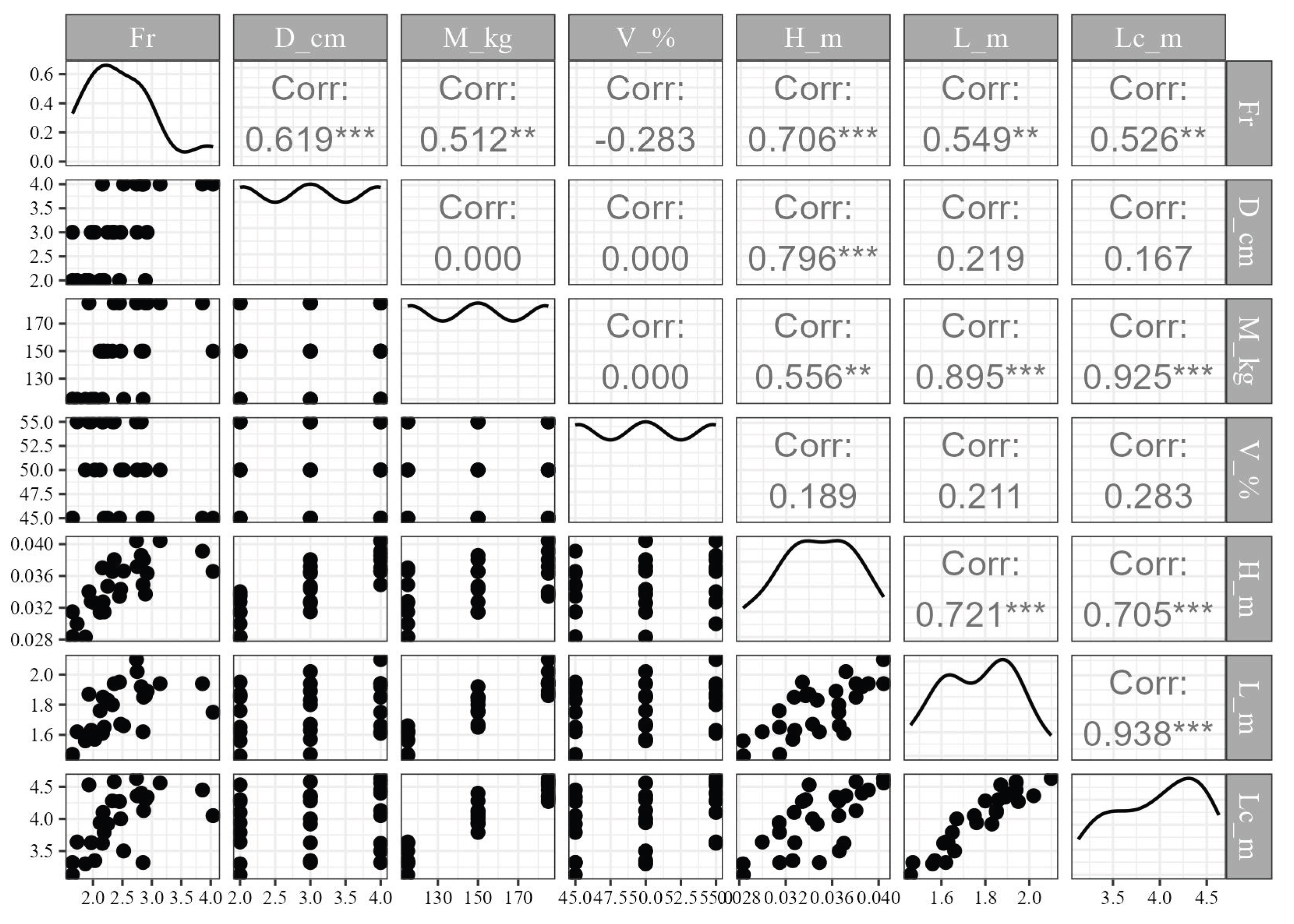
Figure 7.
The erosion depth H (a) and the erosion length L (b) as functions of the point load and the impact energy E of the flow head,respectively.
Figure 7.
The erosion depth H (a) and the erosion length L (b) as functions of the point load and the impact energy E of the flow head,respectively.
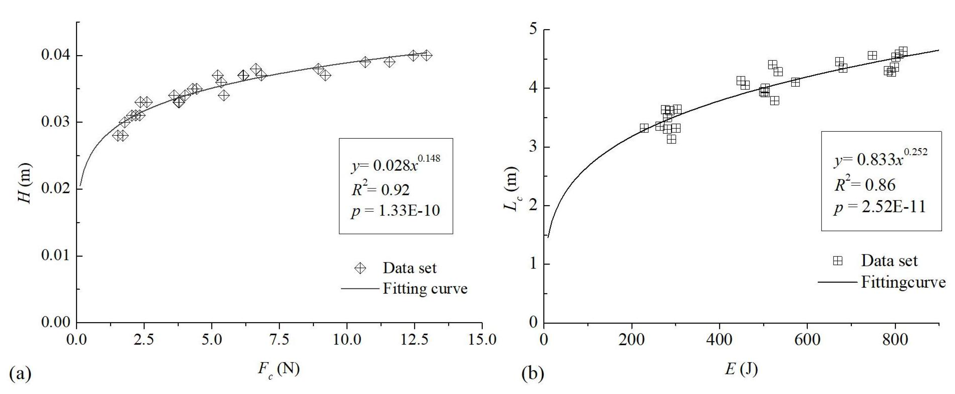
Table 1.
The configuration of parameters for numerical simulations.
| Parameters | Sinking sphere | Erodible bed | Debris flow |
|---|---|---|---|
| Cell size for CFD domain (mm) | 20*20*20 | 60*100*60 | 60*100*60 |
| Mean particle diameter (mm) | 1 | 10 | 20/30/401 |
| Gravity acceleration () | 9.81 | 9.81 | 9.81 |
| Dynamic viscosity of liquid () | 9.81 | 9.81 | 9.81 |
| Message exchange resolution (time steps) | 10 | 10 | 10 |
| Friction coefficient | 0.7 | 0.7 | 0.7 |
| Rebound coefficient | 0.4 | 0.4 | 0.4 |
| Poisson’s ratio | - | 0.3 | 0.3 |
| Time step (sec) | 0.01 | 0.001 | 0.001 |
| Solid fraction | - | 1 | 0.45/0.50/0.55 2 |
1 and 2 denote three different mean diameters and solid fractions, respectively.
Table 2.
representative results from physical and numerical models.
| Results | Physical model | Numerical model |
|---|---|---|
| Pore pressure dissipation time (s) | 38 | 26 |
| Mean flow velocity U (m/s) | 1.32 | 2.30 |
| Mean flow thickness (m) | 0.10 | 0.15 |
| 1.68 | 1.93 | |
| Deposit depth (m) | 0.15 | 0.16 |
| 0.7 | 0.5 |
Table 3.
Experimental variables.
| Solid fraction (%) | Uniform diameter of debris flow (cm) | Total mass (kg) | Serial ID. |
|---|---|---|---|
| 55 | 4 | 115 | D4M115V55 |
| 150 | D4M150V55 | ||
| 185 | D4M185V55 | ||
| 55 | 3 | 115 | D3M115V55 |
| 150 | D3M150V55 | ||
| 185 | D3M185V55 | ||
| 55 | 2 | 115 | D2M115V55 |
| 150 | D2M150V55 | ||
| 185 | D2M185V55 | ||
| 50 | 4 | 115 | D4M115V50 |
| 150 | D4M150V50 | ||
| 185 | D4M185V50 | ||
| 50 | 3 | 115 | D3M115V50 |
| 150 | D3M150V50 | ||
| 185 | D3M185V50 | ||
| 50 | 2 | 115 | D2M115V50 |
| 150 | D2M150V50 | ||
| 185 | D2M185V50 | ||
| 45 | 4 | 115 | D4M115V45 |
| 150 | D4M150V45 | ||
| 185 | D4M185V45 | ||
| 45 | 3 | 115 | D3M115V45 |
| 150 | D3M150V45 | ||
| 185 | D3M185V45 | ||
| 45 | 2 | 115 | D2M115V45 |
| 150 | D2M150V45 | ||
| 185 | D2M185V45 |
e.g. D2M150V45 D2, M150, and V45 denote grain size of 2 cm, total mass of 150 kg, and solid fraction of 45 %, respectively.
Disclaimer/Publisher’s Note: The statements, opinions and data contained in all publications are solely those of the individual author(s) and contributor(s) and not of MDPI and/or the editor(s). MDPI and/or the editor(s) disclaim responsibility for any injury to people or property resulting from any ideas, methods, instructions or products referred to in the content. |
© 2025 by the authors. Licensee MDPI, Basel, Switzerland. This article is an open access article distributed under the terms and conditions of the Creative Commons Attribution (CC BY) license (http://creativecommons.org/licenses/by/4.0/).
Copyright: This open access article is published under a Creative Commons CC BY 4.0 license, which permit the free download, distribution, and reuse, provided that the author and preprint are cited in any reuse.


