
Submitted:
13 September 2025
Posted:
16 September 2025
You are already at the latest version
Abstract
Background/Objectives: This study evaluates photon-counting CT (PCCT) for high-resolution imaging of mouse femurs and investigates how APOE genotype, sex, and humanized nitric oxide synthase (HN) expression influence bone morphology during aging. Methods: A custom-built micro-CT system with a photon-counting detector (PCD) was used to acquire dual-energy scans of mouse femur samples. PCCT projections were corrected for tile gain differences, iteratively reconstructed with 20 µm isotropic resolution, and decomposed into calcium and water maps. PCD performance was benchmarked against an energy-integrating detector (EID) using modulation transfer functions and line profiles. Contrast-to-noise ratio quantified effects of iterative reconstruction and material decomposition. Femur features such as mean cortical thickness, mean trabecular spacing (TbSp_mean), and trabecular bone volume fraction (BV/TV) were extracted from calcium maps using BoneJ. Statistical analysis used 57 aged mice representing APOE22, APOE33, and APOE44 genotypes, including 27 expressing HN. We used generalized linear models (GLMs) to evaluate main and interaction effects of age, sex, genotype, and HN status on femur features and Mann-Whitney U tests for stratified analyses. Results: PCCT outperformed EID-CT in spatial resolution and enabled effective separation of calcium and water. GLMs revealed significant interactions between sex and HN status affecting trabecular features. Female HN mice exhibited reduced BV/TV and increased TbSp_mean compared to both male HN and female non-HN mice. While genotype effects were modest, genotype by sex stratified analysis found significant effects of HN status only in female APOE22 and APOE44 mice. Conclusions: These results demonstrate PCCT’s utility for femur analysis in mice, supporting its application in skeletal disease research.
Keywords:
photon-counting CT
; mice
; bone
1. Introduction
High-resolution bone imaging is critical to understanding the interplay between skeletal integrity and systemic factors such as aging, metabolism, inflammation, and genetic predisposition. X-ray CT is typically used for these studies due to its inherent high contrast for bone imaging. While many previous studies have used conventional micro-CT systems with energy-integrating detectors (EID) to quantify bone architecture, this type of detector has limitations in spatial resolution, beam hardening, and compositional differentiation. Photon-counting computed tomography (PCCT), by contrast, represents a transformative advance. Unlike EID systems that use scintillators to convert x-ray photons into light and then into electrical signals, photon-counting detectors (PCDs) convert each x-ray photon directly into an electrical pulse and count them based on user-defined energy thresholds [1,2]. This results in improved spatial resolution, reduced electronic noise, and multi-energy imaging in a single acquisition [2].
PCCT’s potential for bone imaging has been demonstrated in both clinical and preclinical studies. In cadaveric human bones, PCCT has been shown to improve tissue contrast and reduce metal artifacts compared to dual-energy EID CT [3,4]. Preclinical work using PCCT in rodent models has also shown accurate material decomposition and significant detection of disease-related changes, such as those induced by ovariectomy [5]. However, the application of PCCT to high-resolution bone morphometry in genetically diverse murine models has not yet been fully explored.
Bone health is interconnected with cardiovascular and neurological systems through shared pathways involving apolipoprotein E (APOE) and nitric oxide (NO) [6-9]. APOE, a lipid-transport protein with three isoforms (ε2, ε3, ε4), influences bone formation via lipid metabolism [6]. Genetic variation or deficiency in APOE has been linked to altered bone remodeling [9,10]. While some studies report associations between ε4 and reduced bone mineral density [6,11,12], others find no clear link [13,14], suggesting context-dependent effects.
Mouse models are useful for studying how interactions between risk factors influence bone health because both their genetic background and lifestyle factors such as diet and exercise can be tightly controlled. While prior studies of bone health have used mice with variation in APOE genotype [15,16], incorporating additional variation in immune response via presence or absence of a humanized NOS2 (HN) gene [17] is much less common. NOS2 regulates nitric oxide (NO) production during inflammation, affecting bone remodeling via osteoblast/osteoclast activity and oxidative stress [18].
In this study, we leverage a custom high-resolution PCCT system to image femurs from 57 aged mice with defined homozygous APOE genotypes (APOE22, APOE33, APOE44), including a subset expressing humanized NOS2. We demonstrate the technical performance of PCCT in terms of spatial resolution, contrast to noise ratio, and spectral decomposition. Using calcium maps derived from multi-energy acquisitions, we quantify trabecular and cortical bone features and examine group-level trends linked to sex, immune status, APOE genotype, and age. This work highlights PCCT’s advantages for musculoskeletal research and applies PCCT imaging of mouse femurs to study the complex interactions between risk factors for impaired bone health.
2. Materials and Methods
2.1. Mouse Cohort and Sample Preparation
This study analyzed femurs from 57 aged C57BL/6J mice genetically engineered to express one of three human APOE alleles (ε2, ε3, or ε4) in homozygous form, resulting in 3 distinct APOE genotypes (APOE22, APOE33, APOE44). Of these, 27 mice (47%) also expressed a humanized version of the NOS2 gene (HN), providing an immune background more representative of human physiology [17,19,20]. The cohort included both sexes and spanned an age range of 13.2 to 28.0 months (mean ± SD: 17.8 ± 3.3 months). All animals were maintained on a standard chow diet (LabDiet 5001), with an average body mass of 31.1 ± 4.1 g at the time of imaging. Each APOE genotype group included both male and female mice, though minor sex imbalances occurred in the APOE22HN and APOE44HN subgroups due to breeding constraints. Table 1 summarizes the distribution by genotype, sex, and HN status; Table 2 provides the corresponding age distributions.
All animal procedures were approved by the Duke University Institutional Animal Care and Use Committee (IACUC, Protocol Registry Number: A173-20-08). Mice were euthanized by transcardiac perfusion under deep anesthesia induced by intraperitoneal injection of ketamine/xylazine (100 mg/kg and 10 mg/kg, respectively), as previously described [21]. We ensured that this euthanasia was done humanely with concern for the welfare of the mouse. The left femur was excised, and soft tissues were carefully removed. Femurs from three different mice were embedded in 1% agarose (w/v in PBS) inside 15 mL conical tubes, with rubber bands serving as fiducial markers to help us differentiate between the femurs. Once the gel solidified, the tubes were filled with phosphate-buffered saline (PBS) to preserve hydration and reduce beam hardening during our CT acquisition. The preparation followed recommendations for ex vivo murine femur imaging [22]. Following completion of sample preparation, each vial containing femurs was scanned using PCCT.
2.2. Photon-Counting CT Scanning
All ex vivo imaging was performed using a custom-built micro-CT scanner equipped with two x-ray detectors: a photon-counting detector (PCD) and a conventional energy-integrating detector (EID) [23]. The PCD (XC-Thor, XCounter AB) consists of 8 tiled CdTe-based detector chips with dimensions of 128×256 pixels per tile (1024×256 for whole detector), a pixel size of 100 μm, and two programmable energy thresholds per acquisition. The EID module (Dexela 1512, PerkinElmer) features a 75 μm pixel size and uses a CsI scintillator coupled to a CMOS sensor. The PCD was the primary detector used for high-resolution femur imaging and material decomposition. The EID was included in this study solely for comparison of spatial resolution, as detailed in our previous studies [20,23]. Both detectors are mounted orthogonally to the x-ray source and can be interchanged without altering the scanning geometry [23]. For all PCD scans, the x-ray source was operated at 60 kVp and 134 μA. Data were acquired using a helical trajectory, covering 1400 angular views over 1070° of total rotation with 21 mm of vertical translation. At each projection angle, 100 low-noise exposures of 40 ms were averaged. The PCD energy thresholds were set to 15 keV and 34 keV to optimize sensitivity for calcium and water separation in subsequent material decomposition. With these settings, each vial scan required approximately 2 hours and 6 minutes to complete.
2.3. Artifact Correction
The 8 detector tiles of the XC-Thor PCD have varying spectral response. As a result, the projections have noticeable intensity differences between tiles even after log-normalization, and low frequency concentric bands are present in the reconstructed image [24]. As we have discussed in our prior study on ex-vivo brain imaging [20], we correct this using the multiplicative projection domain water gain correction proposed by Kim and Baek [25], with a PBS vial used in place of a water vial. This procedure involves: (1) acquiring a PCCT scan of a vial filled with only PBS solution using the same trajectory as the femur scanning, (2) constructing artificial PCCT projections on the computer to resemble an ideal PCCT scan of a PBS vial without artifacts, (3) creating PBS gain projections by dividing the ideal PBS projections by the PCCT projections from the real scan of the PBS vial, and (4) Multiplying the PCCT projections from a real scan of a femur sample vial by the PBS gain projections. After this correction of background nonuniformities, the PCD projections from a femur sample vial are ready for reconstruction.
2.4. Image Reconstruction
Since analytical reconstruction of the corrected PCCT projections of a femur sample vial with the weighted filtered backprojection (wFBP) algorithm [26] results in a noisy image, iterative reconstruction is necessary. Accordingly, we performed iterative reconstruction of our PCD projections with two energy thresholds using the Multi-Channel Reconstruction (MCR) Toolkit [27]. Our reconstructed volumes have an isotropic voxel size of 20 μm and about 1000 axial slices with dimensions of 960×960 voxels, although there was some variation in the values of these dimensions to account for changes in position of the vial and the femurs inside it. For iterative reconstruction, we used the split Bregman method with the add-residual-back strategy [28] and rank-sparse kernel regression regularization (RSKR) [27,29], solving the following optimization problem:
Thus, we solve iteratively for the vectorized, reconstructed data, the columns of X, for each energy simultaneously (indexed by e). The reconstruction for each energy minimizes the reprojection error (R, system projection matrix) relative to the log-transformed PCD projection data acquired at each energy (the columns of Y). To reduce noise in the reconstruction, the data fidelity term is minimized subject to the bilateral total variation (BTV) measured within and between energies via RSKR. Each set of 2 energy channel, tile artifact corrected PCD projection data from a femur sample scan was reconstructed using this approach with 4 iterations.
2.5. Material Decomposition
We performed image-based material decomposition of the PCD iterative reconstruction using the method of Alvarez and Macovski [30]. Thus, we performed a post-reconstruction spectral decomposition with H2O and calcium (Ca) as basis functions:
In this formulation, M is a matrix of material sensitivities (attenuation per unit concentration for each material) at each energy. We computed the values in M by scanning and reconstructing a phantom containing a water vial and a vial of 40 mg/mL Ca in water and fitting the slope of attenuation measurements taken in the vials. CH2O represents density in g/mL for H2O, while CCa is the Ca concentration in mg/mL. Finally, X is the attenuation coefficient of the voxel under consideration at energy e. Material decomposition was performed by matrix inversion, solving the following linear system at each voxel:
Orthogonal subspace projection was used to prevent negative concentrations [29]. Post decomposition, the material maps were assigned to colors and visualized in ImageJ.
2.6. Image Quality Assessment
Using one of our femur sample vials, we performed a quantitative assessment of the effects of PBS gain correction and iterative reconstruction. For this sample, we selected a line profile through the center of the vial in the first energy threshold (15 keV) and measured the intensity along this line in the wFBP reconstruction of the uncorrected projections, wFBP reconstruction of the PBS-corrected projections, and iterative reconstruction of the PBS-corrected projections. Then, we computed percent image uniformity (PIU) along each line profile using the following formula.
To compare spatial resolution between photon-counting and energy-integrating detectors, we acquired additional scans of the QRM Micro-CT Bar Pattern Phantom (https://www.qrm.de/) and a representative mouse femur. Both samples were scanned using both the PCD and EID of our micro-CT system described in Section 2.2 with the same helical trajectory and matched acquisition settings: 60 kVp tube voltage, 134 μA current, and an exposure time of 1.2 seconds per projection angle (the maximum allowable for the EID without saturation). The PCD scan used energy thresholds of 15 and 34 keV. All images were reconstructed at 20 μm isotropic voxel size using our iterative reconstruction pipeline to enable direct comparison of PCD and EID data. For the QRM phantom reconstructions, we computed image contrast for the bar patterns with 3.3, 5, 10, and 16.6 line pairs per mm (lp/mm) and fit a Gaussian curve to these measurements to produce modulation transfer functions (MTFs) for the PCD and EID scans. For the femur, we measured the intensity along the same line profile through trabecular bone in both the PCD and EID reconstructions. We then normalized both line profiles by their maximum value and plotted them together to provide a visual assessment of spatial blurring of the trabecular bone.
Finally, using one of our femur samples, we compared image contrast between the PCD wFBP reconstruction, PCD iterative reconstruction, and material decomposition of the PCD iterative reconstruction. We computed contrast to noise ratio (CNR) for each displayed image (PCD 15 keV and PCD 34 keV from both wFBP and iterative reconstructions, Water, Calcium) using the following formula:
where μ1 and σ1 are the mean and standard deviation from a foreground region of interest (ROI) in trabecular bone and μ2 and σ2 are the mean and standard deviation from a background, non-bone ROI inside the femur.
2.7. Femur Feature Extraction
Following iterative reconstruction and material decomposition of each scan, we extracted quantitative features from the calcium material map for each femur using ImageJ and its BoneJ plugin [31]. First, we created separate image volumes that isolate each individual femur in the sample vial by creating a substack of axial slices from a cropped rectangular region of interest in the calcium map. Using this smaller, femur-specific volume, we followed the instructions from use case 2 in the BoneJ manuscript [31] to align the femur to its principal axes and compute mean cortical thickness in two dimensions (MeanThick2D) and in three dimensions (MeanThick3D) from the central axial slice of the femur.
Next, we analyzed the trabecular bone in the metaphyseal region located slightly above the growth plate of the distal femur, as suggested in previous studies of mouse femurs [22,32]. Specifically, we selected a region that is 80 axial slices (1.6 mm) in height, with the bottom slice located 40 slices (0.8 mm) above the center of the growth plate. An example of trabecular region selection is illustrated in the bounding box in Figure 1a. After extracting a metaphyseal substack from the femur specific volume, we used the freehand selection tool in ImageJ to draw manual contours of the region inside the cortical bone on every 10th axial slice, and then we interpolated the ROIs. This results in an 80-slice volume of interest (VOI) with a shape that matches the region inside the cortical bone. Figure 1b shows an example of freehand contour selections on 3 axial slices from the distal metaphyseal substack. By using the “clear” and “clear outside” functions in ImageJ, we defined separate volumes for the trabecular bone inside the contoured VOI and the cortical bone outside the VOI. We performed Otsu’s thresholding on each of these volumes to generate a trabecular mask and a cortical mask, then added them together to create a combined trabecular & cortical mask. The trabecular mask was passed into BoneJ to compute the trabecular bone volume and surface area. Bone volume was divided by the total volume of the 80-slice contoured VOI to compute bone volume fraction (BV/TV). Trabecular spacing (TbSp) and trabecular thickness (TbTh) maps were defined by passing the combined trabecular & cortical mask into the BoneJ thickness function and then clearing the region outside the contoured VOI in the resulting maps. For each of these maps, we then computed the mean across all voxels that do not have value 0 or NaN to obtain TbSp_mean and TbTh_mean. Finally, mean calcium concentration (MeanCaConc) was computed by multiplying the calcium map of the distal metaphyseal VOI by the trabecular mask and taking the mean across all voxels that have a nonzero value.
2.8. Statistical Analysis of Femur Features
After extracting the features described above from each femur, we used statistical methods to understand how these features are influenced by age, sex, APOE genotype, and immune status (HN). Our statistical analysis code, which is included in the online repository for this manuscript (https://gitlab.oit.duke.edu/rohan.nadkarni/pcct-femur-analysis/), used the scipy and statsmodel packages in the Python programming language.
2.8.1. Tests for Normality and Homogeneity of Variance
First, we checked whether each feature followed a normal (bell-shaped) distribution using the Shapiro-Wilk test [33]. In the Shapiro-Wilk test, the null hypothesis is a normal distribution, the alternative hypothesis is a skewed distribution, and the significance level we chose for rejection of the null hypothesis was 5%. Next, we used Levene’s test to check if each femur feature meets the null hypothesis of homogeneity of variances across experimental subgroups [34], with a 5% significance level for rejection of this hypothesis. Table A1 in the Appendix shows the p-values from the Shapiro-Wilk and Levene’s tests. MeanThick2D, MeanThick3D, and MeanCaConc all had a p-value greater than 0.05 in both tests, so we accept the null hypotheses that the feature is normally distributed and has equal variances across subgroups. BV/TV, TbTh_mean, and surface area did not meet the assumption of normal distribution but did meet the assumption of equal variances, while TbSp_mean failed both assumptions.
2.8.2. Multi-factor Generalized Linear Models
Each feature was analyzed using a generalized linear model (GLM), which can easily be adapted for normally distributed or skewed response data by adjusting its two main parameters: (1) the expected probability distribution family of the response variable and (2) the link function used to transform the response variable. Our consistent use of GLMs for both normally distributed and skewed data ensured that the predictors and types of model parameters (coefficient and p-value for each predictor) were identical for all femur features.
Features that were normally distributed and had equal variances across subgroups were analyzed using a GLM with the Gaussian distribution family. The formula for the GLM was:
Feature ~ Age + Sex + Genotype + HN + Age:Sex + Age:Genotype + Age:HN + Sex:Genotype + Sex:HN + Genotype:HN.
In this formula, Feature refers to a femur feature such as MeanThick2D, Genotype refers to classification of mice by APOE with HN status ignored (APOE22, APOE33, or APOE44), and HN refers to classification of mice by HN status with APOE genotype ignored (HN or non-HN). In our model, Age (in months) is a continuous variable, while the remaining 3 independent variables are categorical. For our categorical variables, the reference (level 0) values in our model were Male, APOE33, and non-HN. We included all two-way interactions but excluded higher-order interactions from the GLM formula to simplify interpretation.
For features that failed the Shapiro-Wilk test or both tests, we applied a GLM with the Gamma distribution and a log link function, which is suitable for positively skewed data [35]. These GLMs used the same formula as above.
For all GLMs, p-values were corrected for multiple comparisons using the Benjamini-Hochberg (BH) false discovery rate (FDR) procedure at a 5% threshold [36]. P-values corresponding to a single predictor across all femur features were grouped together during FDR correction. We report coefficients and corrected p-values for significant predictors only.
2.8.3. Stratified Subgroup Analyses
In addition to running GLMs on the entire cohort of 57 mice, we ran several stratified subgroup analyses. First, we separated the data into male-only and female-only and assessed the effect of genotype on each femur feature within these subgroups (Figure A1). Then, we separated the data into HN and non-HN and assessed the effect of genotype on each femur feature within each of those groups (Figure A2). In these stratified analyses, we used the Kruskal-Wallis test [37] to check for differences by genotype, with FDR correction of p-values using the BH method at a 5% significance threshold as described earlier. This test evaluates a null hypothesis of equal medians between three or more groups, making it suitable for femur features that are not necessarily normally distributed after stratification.
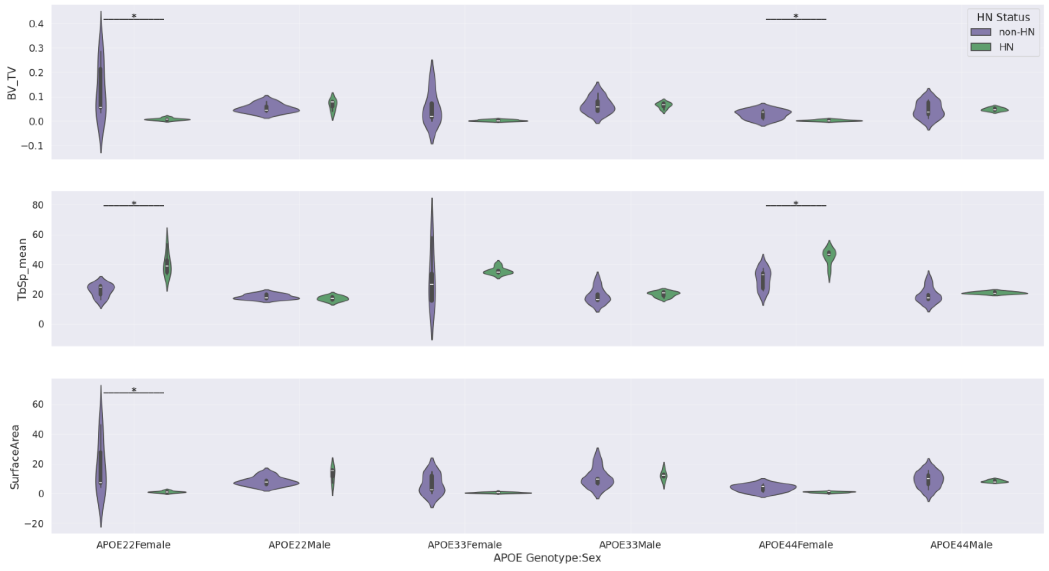
Our other stratified analyses investigated the effects of sex and HN on femur features. We sorted mice into HN and non-HN subgroups and determined if sex has an effect in each group. Conversely, we also sorted mice into male and female subgroups and determined if HN status has an effect in each group. For the femur features with significant difference by HN status in at least one sex specific subgroup, we then sorted mice into genotype by sex subgroups (e.g., APOE22 Female) and assessed the effect of HN status in all six of these groups (Figure A3). Since HN and sex both have just 2 categories, we used the Mann-Whitney U test (Kruskal-Wallis test comparing only two groups) with BH FDR correction of p-values for each of these stratified tests.
Finally, we assessed the effect of age within stratified subgroups. Since age is a continuous variable in our analysis, this was done using linear regression. For each combination of femur feature and categorical variable (sex, APOE genotype, HN), we generated a scatter plot with age on the x-axis and the femur feature (or its natural logarithm if it has a skewed distribution) on the y-axis, with separate color-coding and best fit lines for each level (e.g., Male and Female) of the categorical variable. Unlike the multivariate GLMs discussed earlier, this stratified analysis fitted lines with the simple formula: G(Feature) = m×Age + b. Where G() refers to the log() operation for femur features with a skewed distribution and the identity operation for femur features with a normal distribution. P-values from these regressions were BH FDR-corrected across all features within each categorical level.
2.9. Qualitative Assessment of Trabecular Structure
To validate the accuracy of our trabecular metrics and provide a visualization of differences between femur samples, we used ImageJ’s 3D Viewer plugin to generate 3D renderings of the combined trabecular and cortical bone mask from the distal metaphyseal region of several femur samples. Specifically, we compiled a figure to display two metaphyseal 3D renderings for each combination of sex, APOE genotype, and HN status. For each combination, we arranged the renderings so that the younger mouse is on the left and the older mouse is on the right. For each femur sample selected for rendering, we also display the corresponding bone volume fraction and age.
3. Results
3.1. Image Quality Assessment
Figure 2 demonstrates that both PBS gain correction and iterative reconstruction substantially improved image quality. An axial slice from the 15 keV threshold shows progression from the uncorrected wFBP (Figure 2a) to PBS-corrected wFBP (Figure 2b), and finally to PBS-corrected iterative reconstruction (Figure 2c). Line profiles across the vial reveal increasing PIU across methods: 29.5 (uncorrected), 57.5 (PBS-corrected), and 76.2 (PBS-corrected and iterative). Notably, the iterative reconstruction also eliminated ring and streak artifacts near the femurs through joint regularization across energy thresholds.
Figure 3 compares PCD and EID performance using the QRM Micro-CT Bar Pattern Phantom and a mouse femur. The PCD bar pattern image (Figure 3a) showed improved contrast at higher line pair frequencies (10 and 16.6 lp/mm) compared to the EID image (Figure 3b), consistent with MTF curves showing 10% MTF at 19.44 lp/mm for PCD and 14.54 lp/mm for EID (Figure 3c). In femur images (Figure 3d–e), the PCD clearly delineates bone boundaries with reduced spatial blurring. Line profile analysis (Figure 3f) further confirms a sharper transition and narrower peak for the PCD image. To minimize noise in bone imaging, all PCCT femur scans in our aging study used longer exposure (4 seconds per angle) than the data shown in Figure 3. This longer exposure remained within PCD dynamic range and did not introduce saturation.
Figure 4 shows axial slices of a femur scan across three image types: PBS-corrected wFBP, iterative reconstruction, and material maps from decomposition. While the wFBP 34 keV image exhibits low CNR due to high noise, iterative reconstruction reduces the noise level and preserves bone structure at both energies. Material decomposition further enhances bone separation, with the calcium map achieving the highest CNR among all image types. Minor bone residuals in the water map are visible, likely due to partial volume effects or basis material limitations.
3.2. Statistical Analysis of Femur Features
3.2.1. Multi-factor Generalized Linear Models
Table 3 shows all significant predictors from our GLMs applied to the entire cohort of mice (n=57).
Significant predictors were found only for trabecular bone volume fraction (BV/TV) and surface area. Notably, a change from the reference genotype (APOE33) to APOE44 was associated with increased BV/TV (p = 0.00976). The most pronounced effect was observed for the interaction between sex and HN status: female HN mice exhibited significantly lower BV/TV and surface area compared to both HN males and non-HN females (p < 1e-5 for both features). Age also interacted with genotype, such that APOE44 mice showed a steeper decline in BV/TV with increasing age than APOE33 mice (p = 0.00518). While age was a predictor only in this interaction term, we note that APOE44 and APOE44HN groups had slightly higher mean ages than APOE33 and APOE33HN, which may have contributed to this result.
Violin plots in Figure 5a show the full BV/TV distribution across APOE genotypes. While visual differences between genotypes were modest, the GLM for BV/TV revealed significant effects. To control for confounding variables, Figure 5b shows BV/TV residuals from a GLM that excluded genotype effects; these plots further illustrate reduced BV/TV in APOE33 and APOE22 compared to APOE44.
These findings underscore the importance of sex, APOE genotype, and immune background in determining trabecular bone structure in aged mice.
3.2.2. Stratified Subgroup Analyses
In our Kruskal-Wallis tests, we did not find a significant difference in femur features by APOE genotype within the male only, female only, non-HN only, or HN only subgroups. The violin plots associated with these results are shown in the Appendix section in Figure A1 and Figure A2.
Our Mann-Whitney U tests comparing femurs features by sex within HN and non-HN subgroups and by HN status within female and male subgroups returned several statistically significant differences. These significant results are reported in Table 4, and the corresponding violin plots are shown in Figure 6 and Figure 7.
The two figures indicate that: 1) female mice that express the HN gene have significantly less trabecular bone mass (i.e., smaller BV/TV and surface area and larger TbSp_mean) than male mice that express the HN gene and 2) female mice that express the HN gene have significantly less trabecular bone mass than female mice that do not express the HN gene. However, our plots and Mann-Whitney U tests do not show significant differences in femur features between female non-HN and male non-HN or between male HN and male non-HN.
Table 5 highlights the statistically significant findings from our Mann-Whitney U tests for differences in femur features by HN status within genotype-by-sex subgroups. Only three femur features were considered in this analysis—BV/TV, TbSp_mean, and surface area—since these were the only features that showed significant HN effects in our sex stratified analysis (Figure 7).
Significant differences by HN status were found for all 3 femur features in APOE22 females and for BV/TV and TbSp_mean in APOE44 females. In contrast, no significant differences by HN status were observed in APOE33 females or in any of the male subgroups.
These results indicate that the HN-associated bone loss in females is modulated by genotype, with APOE22 and APOE44 backgrounds showing the strongest effect. This three-way interaction (genotype:sex:HN) supports the notion that inflammatory signaling (modeled by HN expression) interacts with genetic susceptibility and sex to influence trabecular bone health in aging. The violin plots corresponding to the comparisons in Table 5 are shown in the Appendix section in Figure A3, providing a visual summary of how HN effects differ by genotype and sex.
In our linear regression with age on the x-axis and femur feature on the y-axis within subgroups defined by sex, HN status, or APOE genotype, only the male subgroup showed statistically significant regression lines after BH FDR correction. Specifically, male mice showed a significant decrease in cortical thickness (both 2D and 3D measures) and a significant increase in trabecular spacing (log-transformed TbSp_mean) with increasing age. Scatter plots illustrating these relationships, including regression lines, r² values, confidence intervals, and corrected p-values, are shown in Figure 8.
No other subgroups —females, HN mice, non-HN mice, or any APOE genotype groups—exhibited significant age-dependent changes in the examined femur features after multiple testing correction. Furthermore, the interaction term Age:Sex was not significant in the full-cohort GLMs, suggesting that the age-related differences observed in males did not extend to females in this cohort.
These findings support a sex-specific aging trajectory, where male mice exhibit more pronounced bone deterioration with age, while female mice may be more affected by inflammatory and genetic interactions (e.g., HN and APOE effects).
3.3. Qualitative Assessment of Trabecular Structure
In Figure 9a, we show 3D renderings of the distal femoral metaphyseal region from 24 representative mice spanning all combinations of APOE genotype, sex, and HN status. These visualizations provide a qualitative perspective on trabecular bone morphology and help contextualize the quantitative metrics. Accompanying heatmaps display the corresponding bone volume fraction (BV/TV, Figure 9b) and age (Figure 9c) for each sample.
The 3D renderings confirm key trends observed in the statistical analysis. Female HN mice consistently exhibit sparser and more fragmented trabecular structures than either male HN mice or female non-HN mice. In contrast, male mice—both with and without HN expression—display more robust and interconnected trabecular networks. These observations are visually striking and align closely with the results from GLMs and subgroup analyses. Some differences between males and females in the non-HN group were also apparent in the renderings. However, these did not reach statistical significance, possibly due to the thicker trabeculae observed in female non-HN mice, which may partially offset the reduced number of trabecular elements.
Overall, the qualitative visualizations in Figure 9 reinforce the conclusion that sex and HN status jointly influence trabecular architecture, particularly in female mice.
4. Discussion
Our image quality assessments demonstrated the efficacy of the photon-counting CT based femur image acquisition and processing procedure. As illustrated in Figure 2, our application of PBS gain correction followed by iterative reconstruction results in femur sample images with minimal background nonuniformity and streak artifacts as well as low noise level. Figure 3 displays equivalent dose PCD and EID reconstructions from scans on our ex vivo micro-CT system that proved that the PCD has superior spatial resolution in a bar pattern phantom and less spatial blurring of bone in a femur sample. We demonstrated in Figure 4 that material decomposition of the multi-energy PCD iterative reconstruction produces a calcium map that has better contrast between trabeculae and background compared to the PCD CT images. These results show that our combination of multi-energy photon-counting CT imaging and iterative reconstruction with joint regularization of energy channels works well. Material decomposition further enhanced image interpretability by isolating calcium content, which is directly correlated with bone density. The calcium maps generated in this study demonstrated the highest CNR (Figure 4), ensuring precise delineation of trabecular structures.
Using this pipeline, we quantified femur features (e.g., BV/TV, TbSp_mean, MeanThick2D/3D) across 57 mice with variation in APOE genotype, sex, HN status, and age. Our GLMs identified significant Sex:HN interaction effects on BV/TV and Surface Area and found APOE44 to be associated with increased BV/TV relative to APOE33 (Figure 5). The result for APOE44 mice is contrary to initial expectations that the ε4 allele—linked to neurodegeneration—would have negative effects on bone. While this finding diverges from younger cohorts in prior literature [15], it underscores the importance of studying aging-specific effects and considering immune context (HN status).
Stratified subgroup analyses revealed pronounced sex-specific HN effects on trabecular bone mass. Specifically, female HN mice had significantly reduced BV/TV, increased trabecular spacing, and smaller trabecular surface area compared to both male HN mice and female non-HN mice (Figure 6 and Figure 7, Table 4). This suggests that the humanized immune background in HN mice modulates sex differences in bone remodeling—likely via inflammatory or hormonal pathways [38]. Notably, these effects were not statistically significant in APOE33 females (Table 5), indicating genotype-specific modulation of HN influence.
Aging was associated with cortical thinning and increased trabecular spacing in males (Figure 8), but not females. This may reflect the earlier onset of bone loss in female mice, potentially masking progressive changes over time. Age–sex interaction terms were not significant in whole-cohort GLMs, possibly due to strong interactions with HN in female mice.
3D renderings of trabecular architecture (Figure 9) visually reinforced quantitative findings, particularly the stark contrast between female HN and male HN bones. These renderings also suggest that statistical non-significance in some subgroups (e.g., female non-HN vs male non-HN) may arise from variation in trabecular thickness rather than number of trabeculae.
C From a biological perspective, our results emphasize that APOE genotype alone has limited predictive power for bone health, aligning with some human studies [14]. Instead, the interaction between genotype, sex, and immune status (HN) was critical in our study. These findings support the use of HN mice in preclinical studies of bone disease, especially for capturing sex-specific vulnerabilities.
Our study complements prior work using PCCT to evaluate cardiac function in APOE/HN mice [39]. Together, the cardiac and bone findings point toward systemic effects of APOE and immune background across multiple organ systems. Both studies implicate shared mechanisms, e.g., inflammation, oxidative stress, lipid metabolism, driving organ remodeling with age. This supports the broader utility of PCCT as a multi-organ phenotyping platform in aging research.
One shortcoming that we acknowledge is that reconstructions from our micro-CT system have a larger voxel size (20 μm) than reconstructions from high quality commercial EID-based micro-CT scanners (~5 μm). This is because of the limited field-of-view of our PCD combined with our desire to perform high-throughput imaging by scanning multiple femurs (i.e., 3) in each vial. Nevertheless, this study demonstrates that properties of the PCD, such as reduced spatial blurring due to direct x-ray photon detection and simultaneous multi-energy imaging, are useful for bone imaging. Future work that incorporates the PCD into commercial micro-CT scanners that can achieve voxel sizes less than 10 μm will be critical to ensure that the benefits of photon-counting CT for small animal bone imaging are fully realized.
Another shortcoming is the size of our study cohort (n=57). Although this sample size is sufficiently large for our whole-cohort GLMs and stratified tests involving sex/HN interaction (Figure 6 and Figure 7), our investigation of HN effects in genotype-by-sex subgroups (Table 5 and Figure A3) may require validation in a larger mouse cohort.
5. Conclusions
We present a validated, high-resolution PCCT pipeline for ex vivo bone imaging in aged mice. Our image quality assessments confirmed that the PCD provides higher spatial resolution than matched dose EID images and that material decomposition of PCD images improves contrast to noise ratio. We used our PCCT pipeline to show that trabecular bone metrics are significantly impacted by interactions between sex and immune (HN) background, with modulation of this effect by APOE genotype. These findings extend the utility of PCCT beyond single-organ applications and highlight the complex, multi-factorial influences on bone health in aging. The methodological and biological insights gained here lay the groundwork for future multi-organ studies using PCCT in preclinical models of aging and disease.
Author Contributions
Conceptualization, R.N., A.B., and C.T.B.; methodology, R.N., Z.Y.H., A.B., and C.T.B.; software, R.N., A.J.A., and D.P.C.; validation, R.N.; formal analysis, R.N.; investigation, R.N. and Z.Y.H.; resources, A.J.A., D.P.C., A.B. and C.T.B.; data curation, R.N. and Z.Y.H.; writing—original draft preparation, R.N.; writing—review and editing, R.N., Z.Y.H., A.J.A., D.P.C., A.B., and C.T.B.; visualization, R.N.; supervision, A.B and C.T.B.; project administration, A.B. and C.T.B.; funding acquisition, A.B. and C.T.B. All authors have read and agreed to the published version of the manuscript.
Funding
This research was performed at the Duke University Quantitative Imaging and Analysis Lab funded by NIH grants number RF1 AG057895, R01 AG066184, and R01 AG070149.
Institutional Review Board Statement
The animal work was conducted under a protocol approved by the Duke University Institutional Animal Care and Use Committee (IACUC). Duke IACUC Protocol Registry Number: A173-20-08. Mice were euthanized by transcardiac perfusion under deep anesthesia induced by intraperitoneal injection of ketamine/xylazine (100 mg/kg and 10 mg/kg, respectively). We ensured that this euthanasia was done humanely with concern for the welfare of the mouse.
Informed Consent Statement
Not applicable.
Data Availability Statement
Data from this study is available on the following public Gitlab repository: https://gitlab.oit.duke.edu/rohan.nadkarni/pcct-femur-analysis.
Acknowledgments
We acknowledge Dr. Yi Qi (Duke Radiology) for supporting our animal research.
Conflicts of Interest
The authors declare no conflicts of interest.
Appendix A

Table A1.
Results of Shapiro-Wilk and Levene’s tests on each femur feature.
| Femur Feature | Shapiro-Wilk p-value | Levene p-value |
|---|---|---|
| MeanThick 2D | 0.5626 | 0.8362 |
| MeanThick 3D | 0.5977 | 0.7124 |
| BV/TV | < 10-4 | 0.0556 |
| TbTh_mean | 0.0025 | 0.6208 |
| TbSp_mean | 0.0020 | 0.0360 |
| Surface Area | < 10-4 | 0.0908 |
| Mean Ca Conc | 0.1799 | 0.9911 |
Figure A1.
Violin plots corresponding to Kruskal-Wallis comparisons by APOE genotype within male and female subgroups. None of the plots include a bar with asterisk because our Kruskal-Wallis tests did not find any femur features with significant difference by genotype within the male subgroup or the female subgroup.
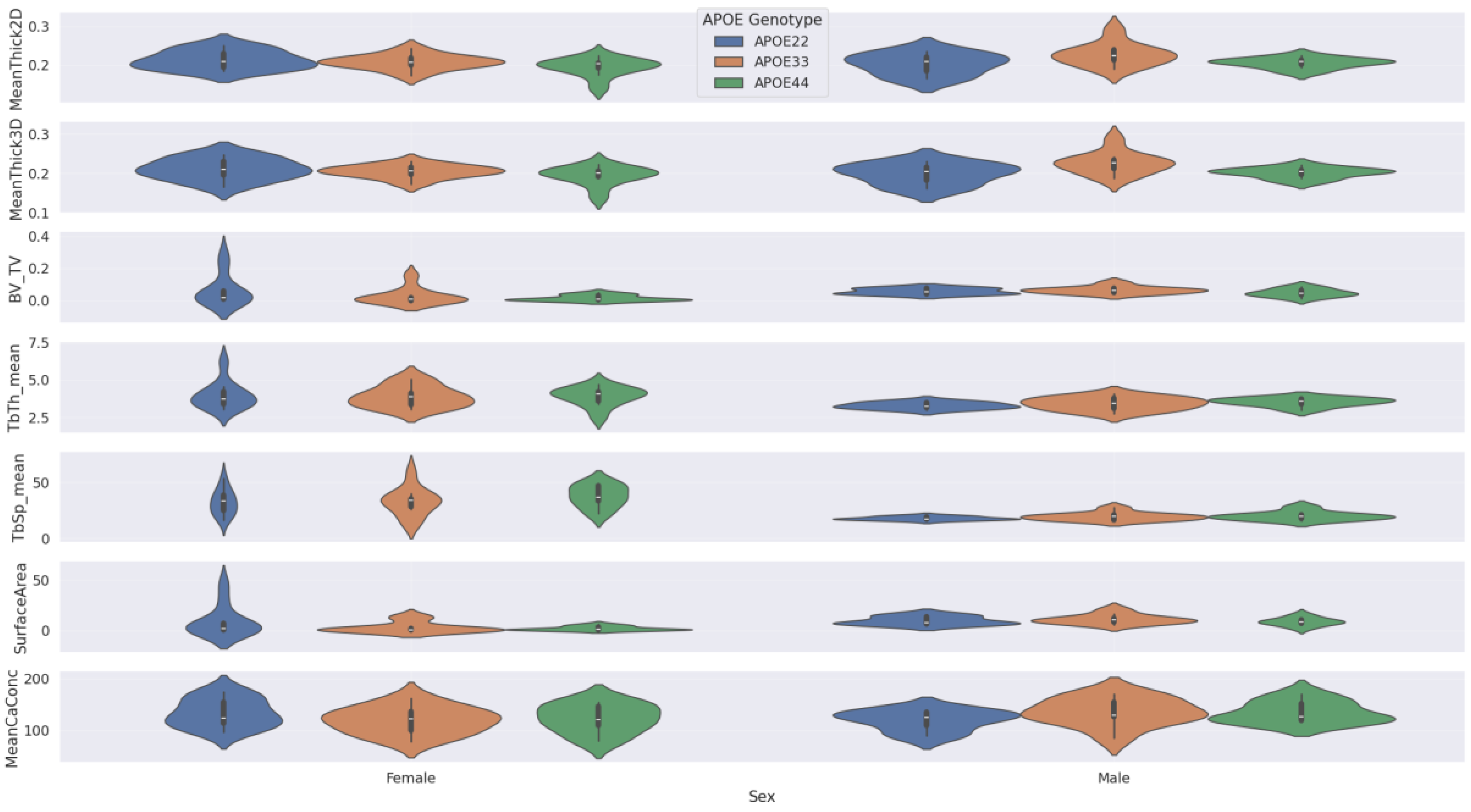
Figure A2.
Violin plots corresponding to Kruskal-Wallis comparisons by APOE genotype within HN and non-HN subgroups. None of the plots include a bar with asterisk because our Kruskal-Wallis tests did not find any femur features with significant difference by genotype within the HN subgroup or the non-HN subgroup.
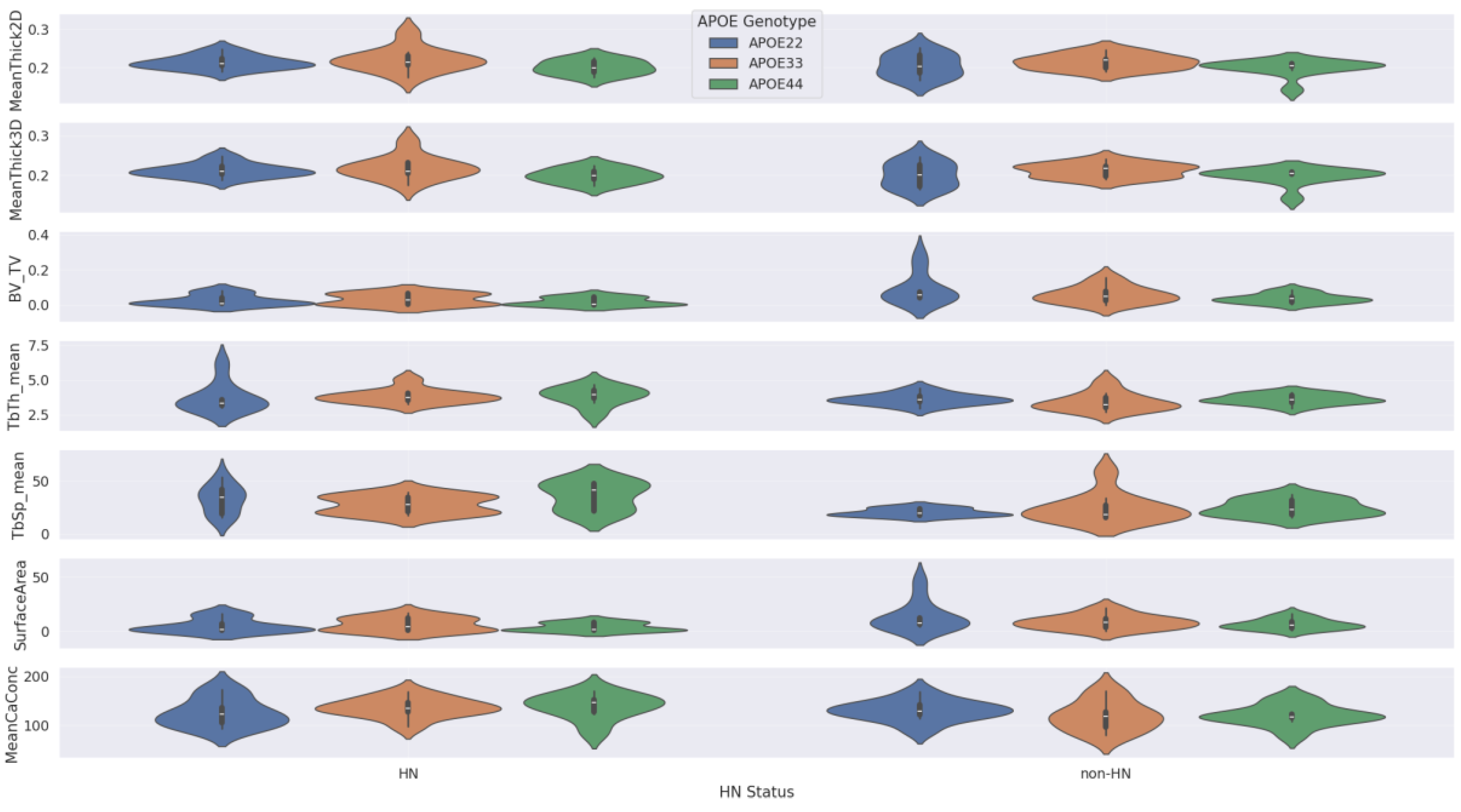
Figure A3.
Violin plots corresponding to Mann-Whitney U comparisons by HN status within genotype by sex subgroups. Bars with an asterisk indicate statistically significant difference (p<0.05) by HN status after BH FDR correction. Only femur features that gave significant difference by HN status in at least one sex specific subgroup in Figure 7 were included in this figure.
References
- Taguchi, K.; Iwanczyk, J.S. Vision 20/20: Single photon counting x-ray detectors in medical imaging. Med Phys. 2013, 40, 100901. [Google Scholar] [CrossRef] [PubMed]
- Leng, S.; Bruesewitz, M.; Tao, S.; Rajendran, K.; Halaweish, A.F.; Campeau, N.G.; Fletcher, J.G.; McCollough, C.H. Photon-counting Detector CT: System Design and Clinical Applications of an Emerging Technology. RadioGraphics 2019, 39, 729–743. [Google Scholar] [CrossRef]
- Fukuda, T.; Yonenaga, T.; Akao, R.; Hashimoto, T.; Maeda, K.; Shoji, T.; Shioda, S.; Ishizaka, Y.; Ojiri, H. Comparison of Bone Evaluation and Metal Artifact between Photon-Counting CT and Five Energy-Integrating-Detector CT under Standardized Conditions Using Cadaveric Forearms. Diagnostics 2024, 14, 350. [Google Scholar] [CrossRef]
- Azari, F.; Uniyal, P.; Soete, J.; Coudyzer, W.; Wyers, C.E.; Quintiens, J.; Bergh, J.P.v.D.; van Lenthe, G.H. Accuracy of photon-counting computed tomography for the measurement of bone quality in the knee. Bone 2024, 181, 117027. [Google Scholar] [CrossRef] [PubMed]
- Bhattarai, A.; Tanaka, R.; Yeung, A.W.K.; Vardhanabhuti, V. Photon-Counting CT Material Decomposition in Bone Imaging. J. Imaging 2023, 9, 209. [Google Scholar] [CrossRef]
- Niemeier, A.; Schinke, T.; Heeren, J.; Amling, M. The role of Apolipoprotein E in bone metabolism. Bone 2011, 50, 518–524. [Google Scholar] [CrossRef]
- Hof, R.J.V.; Ralston, S.H. Nitric oxide and bone. Immunology 2001, 103, 255–261. [Google Scholar] [CrossRef]
- Bartelt, A.; Beil, F.T.; Schinke, T.; Roeser, K.; Ruether, W.; Heeren, J.; Niemeier, A. Apolipoprotein E-dependent inverse regulation of vertebral bone and adipose tissue mass in C57Bl/6 mice: Modulation by diet-induced obesity. Bone 2010, 47, 736–745. [Google Scholar] [CrossRef]
- Hirasawa, H.; Tanaka, S.; Sakai, A.; Tsutsui, M.; Shimokawa, H.; Miyata, H.; Moriwaki, S.; Niida, S.; Ito, M.; Nakamura, T. ApoE Gene Deficiency Enhances the Reduction of Bone Formation Induced by a High-Fat Diet Through the Stimulation of p53-Mediated Apoptosis in Osteoblastic Cells. J. Bone Miner. Res. 2007, 22, 1020–1030. [Google Scholar] [CrossRef]
- Peter, I.; Crosier, M.D.; Yoshida, M.; Booth, S.L.; Cupples, L.A.; Dawson-Hughes, B.; Karasik, D.; Kiel, D.P.; Ordovas, J.M.; Trikalinos, T.A. Associations of APOE gene polymorphisms with bone mineral density and fracture risk: a meta-analysis. Osteoporos. Int. 2010, 22, 1199–1209. [Google Scholar] [CrossRef] [PubMed]
- Shiraki, M.; Shiraki, Y.; Aoki, C.; Hosoi, T.; Inoue, S.; Kaneki, M.; Ouchi, Y. Association of Bone Mineral Density with Apolipoprotein E Phenotype. J. Bone Miner. Res. 1997, 12, 1438–1445. [Google Scholar] [CrossRef] [PubMed]
- Sanada, M.; Nakagawa, H.; Kodama, I.; Sakasita, T.; Ohama, K. Apolipoprotein E phenotype associations with plasma lipoproteins and bone mass in postmenopausal women. Climacteric 1998, 1, 188–195. [Google Scholar] [CrossRef] [PubMed]
- Lui, L.; Stone, K.; Cauley, J.A.; Hillier, T.; Yaffe, K. Bone Loss Predicts Subsequent Cognitive Decline in Older Women: The Study of Osteoporotic Fractures. J. Am. Geriatr. Soc. 2003, 51, 38–43. [Google Scholar] [CrossRef]
- Schoofs, M.W.; van der Klift, M.; Hofman, A.; van Duijn, C.M.; Stricker, B.H.; AP Pols, H.; Uitterlinden, A.G. ApoE Gene Polymorphisms, BMD, and Fracture Risk in Elderly Men and Women: The Rotterdam Study. J. Bone Miner. Res. 2004, 19, 1490–1496. [Google Scholar] [CrossRef]
- Dieckmann, M.; Beil, F.T.; Mueller, B.; Bartelt, A.; Marshall, R.P.; Koehne, T.; Amling, M.; Ruether, W.; A Cooper, J.; E Humphries, S.; et al. Human apolipoprotein E isoforms differentially affect bone mass and turnover in vivo. J. Bone Miner. Res. 2012, 28, 236–245. [Google Scholar] [CrossRef] [PubMed]
- Schilling, A.F.; Schinke, T.; Münch, C.; Gebauer, M.; Niemeier, A.; Priemel, M.; Streichert, T.; Rueger, J.M.; Amling, M. Increased Bone Formation in Mice Lacking Apolipoprotein E. J. Bone Miner. Res. 2005, 20, 274–282. [Google Scholar] [CrossRef]
- Hoos, M.D.; Vitek, M.P.; A Ridnour, L.; Wilson, J.; Jansen, M.; Everhart, A.; A Wink, D.; A Colton, C. The impact of human and mouse differences in NOS2 gene expression on the brain’s redox and immune environment. Mol. Neurodegener. 2014, 9, 50–50. [Google Scholar] [CrossRef]
- Wink, D.A.; Mitchell, J.B. Chemical biology of nitric oxide: insights into regulatory, cytotoxic, and cytoprotective mechanisms of nitric oxide. Free. Radic. Biol. Med. 1998, 25, 434–456. [Google Scholar] [CrossRef]
- Badea, A.; Wu, W.; Shuff, J.; Wang, M.; Anderson, R.J.; Qi, Y.; Johnson, G.A.; Wilson, J.G.; Koudoro, S.; Garyfallidis, E.; et al. Identifying Vulnerable Brain Networks in Mouse Models of Genetic Risk Factors for Late Onset Alzheimer’s Disease. Front. Neurosci. 2019, 13, 72. [Google Scholar] [CrossRef]
- Nadkarni, R.; Han, Z.Y.; Anderson, R.J.; Allphin, A.J.; Clark, D.P.; Badea, A.; Badea, C.T.; Bamorovat, M. High-resolution hybrid micro-CT imaging pipeline for mouse brain region segmentation and volumetric morphometry. PLOS ONE 2024, 19, e0303288. [Google Scholar] [CrossRef]
- Winter, S.; Mahzarnia, A.; Anderson, R.J.; Han, Z.Y.; Tremblay, J.; Stout, J.A.; Moon, H.S.; Marcellino, D.; Dunson, D.B.; Badea, A. Brain network fingerprints of Alzheimer's disease risk factors in mouse models with humanized APOE alleles. Magn. Reson. Imaging 2024, 114, 110251. [Google Scholar] [CrossRef]
- Kim, Y.; Brodt, M.D.; Tang, S.Y.; Silva, M.J. MicroCT for scanning and analysis of mouse bones. Methods Mol. Biol. 2021, 2230, 169–198. [Google Scholar] [CrossRef]
- Allphin, A.J.; Nadkarni, R.; Clark, D.P.; Badea, C.T.; Gimi, B.S.; Krol, A. Ex vivo high-resolution hybrid micro-CT imaging using photon counting and energy integrating detectors. Biomedical Applications in Molecular, Structural, and Functional Imaging. LOCATION OF CONFERENCE, United StatesDATE OF CONFERENCE; pp. 194–199.
- Feng, M.; Ji, X.; Zhang, R.; Treb, K.; Dingle, A.M.; Li, K. An experimental method to correct low-frequency concentric artifacts in photon counting CT. Phys. Med. Biol. 2021, 66, 175011. [Google Scholar] [CrossRef] [PubMed]
- Kim, D.; Baek, J. Comparison of Flat Field Correction Methods for Photon-Counting Spectral CT Images. 2018 IEEE Nuclear Science Symposium and Medical Imaging Conference (NSS/MIC). LOCATION OF CONFERENCE, AustraliaDATE OF CONFERENCE; pp. 1–3.
- Stierstorfer, K.; Rauscher, A.; Boese, J.; Bruder, H.; Schaller, S.; Flohr, T. Weighted FBP—a simple approximate 3D FBP algorithm for multislice spiral CT with good dose usage for arbitrary pitch. Phys. Med. Biol. 2004, 49, 2209–2218. [Google Scholar] [CrossRef] [PubMed]
- Stierstorfer, K.; Rauscher, A.; Boese, J.; Bruder, H.; Schaller, S.; Flohr, T. Weighted FBP—a simple approximate 3D FBP algorithm for multislice spiral CT with good dose usage for arbitrary pitch. Phys. Med. Biol. 2004, 49, 2209–2218. [Google Scholar] [CrossRef]
- Clark, D.P.; Badea, C.T. MCR toolkit: A GPU-based toolkit for multi-channel reconstruction of preclinical and clinical x-ray CT data. Med Phys 2023, 10.1002/mp. 1653. [Google Scholar] [CrossRef]
- Gao, H.; Yu, H.; Osher, S.; Wang, G. Multi-energy CT based on a prior rank, intensity and sparsity model (PRISM). Inverse Probl. 2011, 27. [Google Scholar] [CrossRef]
- Clark, D.P.; Badea, C.T. Hybrid spectral CT reconstruction. PLOS ONE 2017, 12, e0180324–e0180324. [Google Scholar] [CrossRef] [PubMed]
- E Alvarez, R.; Macovski, A. Energy-selective reconstructions in X-ray computerised tomography. Phys. Med. Biol. 1976, 21, 733–744. [Google Scholar] [CrossRef]
- Doube, M.; Kłosowski, M.M.; Arganda-Carreras, I.; Cordelières, F.P.; Dougherty, R.P.; Jackson, J.S.; Schmid, B.; Hutchinson, J.R.; Shefelbine, S.J. BoneJ: Free and extensible bone image analysis in ImageJ. Bone 2010, 47, 1076–1079. [Google Scholar] [CrossRef]
- Shim, J.; Iwaya, C.; Ambrose, C.G.; Suzuki, A.; Iwata, J. Micro-computed tomography assessment of bone structure in aging mice. Sci. Rep. 2022, 12, 1–16. [Google Scholar] [CrossRef]
- Shapiro, S.S.; Wilk, M.B. An Analysis of Variance Test for Normality (Complete Samples). Biometrika 1965, 52, 591. [Google Scholar] [CrossRef]
- Zimmerman, D.W. A note on preliminary tests of equality of variances. Br. J. Math. Stat. Psychol. 2004, 57, 173–181. [Google Scholar] [CrossRef]
- Ng, V.K.; Cribbie, R.A. Using the Gamma Generalized Linear Model for Modeling Continuous, Skewed and Heteroscedastic Outcomes in Psychology. Curr. Psychol. 2016, 36, 225–235. [Google Scholar] [CrossRef]
- Benjamini, Y.; Hochberg, Y. Controlling the False Discovery Rate: A Practical and Powerful Approach to Multiple Testing. J. R. Stat. Soc. Ser. B Methodol. 1995, 57, 289–300. [Google Scholar] [CrossRef]
- Kruskal, W.H.; Wallis, W.A. Use of Ranks in One-Criterion Variance Analysis. J. Am. Stat. Assoc. 1952, 47, 583–621. [Google Scholar] [CrossRef]
- Mills, E.G.; Yang, L.; Nielsen, M.F.; Kassem, M.; Dhillo, W.S.; Comninos, A.N. The Relationship Between Bone and Reproductive Hormones Beyond Estrogens and Androgens. Endocr. Rev. 2021, 42, 691–719. [Google Scholar] [CrossRef]
- Allphin, A.J.; Mahzarnia, A.; Clark, D.P.; Qi, Y.; Han, Z.Y.; Bhandari, P.; Ghaghada, K.B.; Badea, A.; Badea, C.T.; Faggioni, L. Advanced photon counting CT imaging pipeline for cardiac phenotyping of apolipoprotein E mouse models. PLOS ONE 2023, 18, e0291733. [Google Scholar] [CrossRef]
Figure 1.
Region selections for femur processing. (a) Coronal view of a cropped femur specific volume of interest from the calcium map. The yellow line at the center of the femur shows the location at which mean cortical thickness was computed, while the yellow bounding box near the bottom of the femur shows the location of the metaphyseal volume of interest from which trabecular metrics were computed. (b) First (top), 40th (center) and 80th (bottom) axial slice of metaphyseal region, with contours of the boundary of the trabecular region shown in yellow. Both the coronal femur image in (a) and the 1st axial slice of the metaphyseal region in (b) include scale bars to show a length of 1 mm on the image.
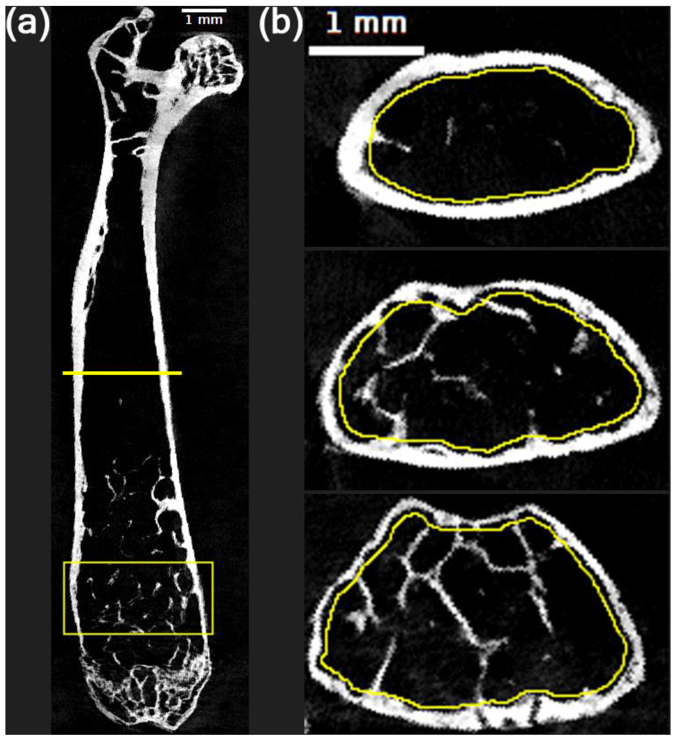
Figure 2.
Effects of PBS gain correction and iterative reconstruction in an axial slice from the 15 keV energy threshold of a vial with 3 femurs. (a) wFBP reconstruction of PCD projection before PBS gain correction (b) wFBP reconstruction of PBS gain corrected PCD projection (c) Iterative reconstruction of PBS gain corrected PCD projection. The plot to the right of each image shows the attenuation values along the yellow line profile overlayed on the image. The calibration bar in (a) shows the display setting for all images in units of cm-1.
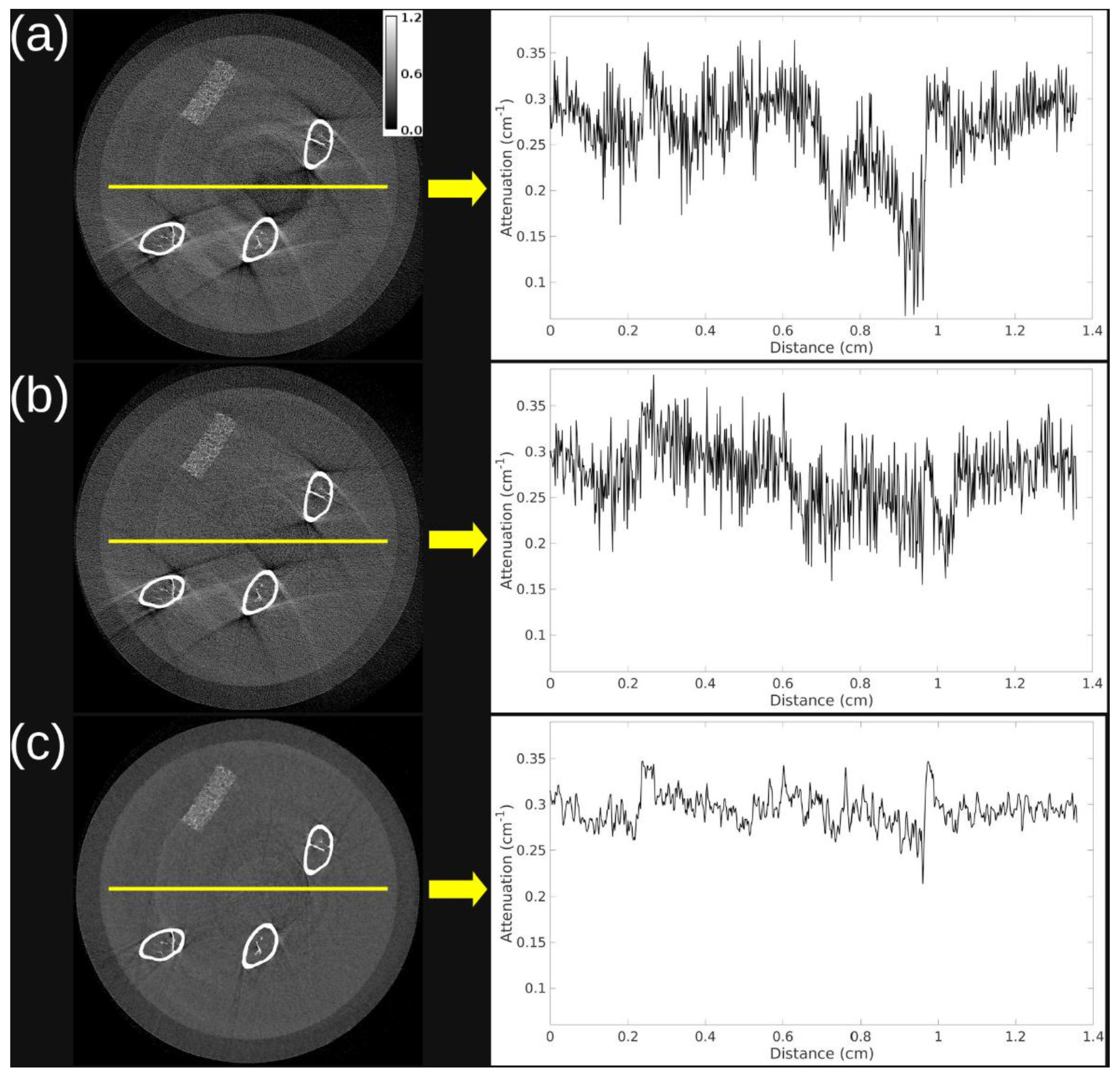
Figure 3.
Spatial resolution assessment of PCD and EID scans on our ex vivo micro-CT system using the QRM Micro-CT Bar Pattern Phantom and a femur sample. (a) PCD iterative reconstruction of QRM phantom at first energy threshold (b) EID iterative reconstruction of QRM phantom (c) modulation transfer function (MTF) curves from PCD and EID QRM phantom reconstructions (d) PCD iterative reconstruction of femur sample at first energy threshold (e) EID iterative reconstruction of same femur sample (f) Plot of attenuation normalized by maximum value along dashed red line profile in (d) in PCD and EID reconstructions. The calibration bars in (a), (b), (d), and (e) show the display settings for these images in units of cm-1.
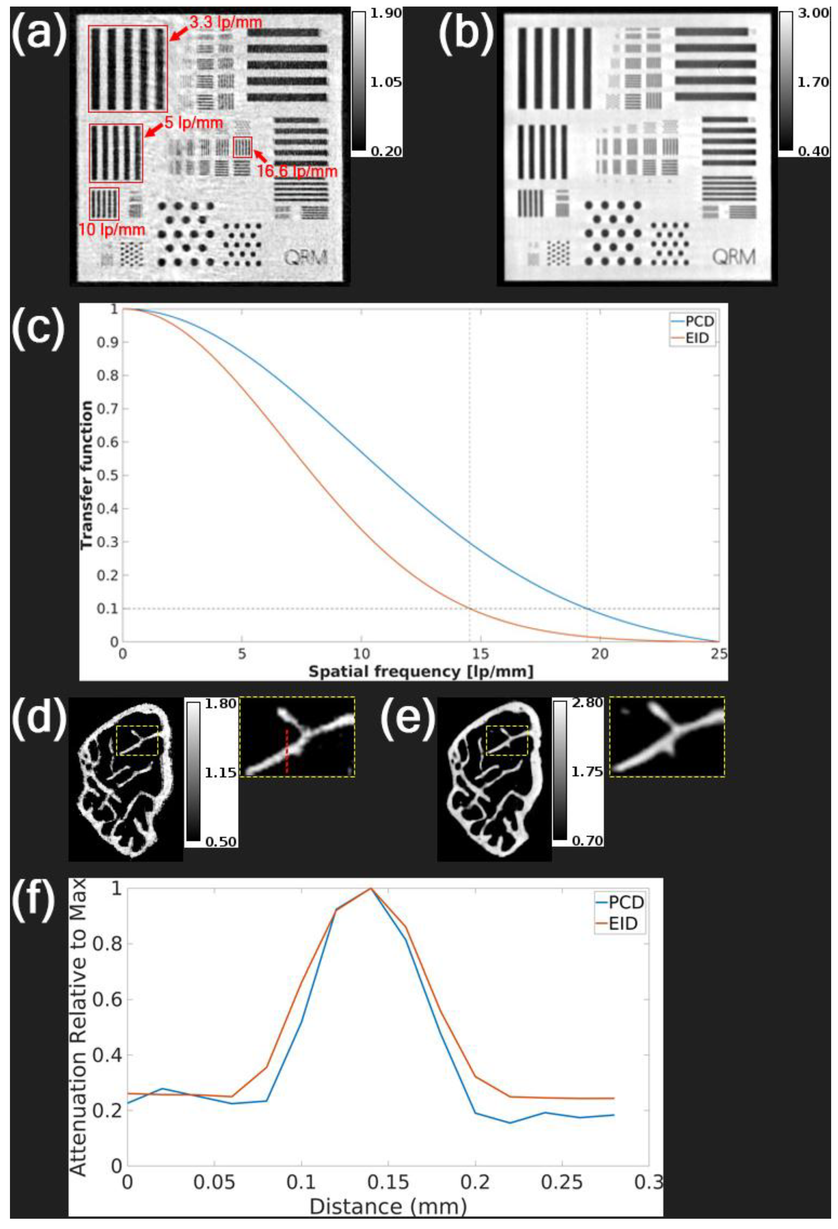
Figure 4.
Axial slice from reconstruction and material decomposition of vial with mouse femurs. (a) wFBP reconstruction at both energy thresholds. (b) Iterative reconstruction at both energy thresholds. (c) Water and calcium maps from material decomposition of iterative reconstruction. (d) Contrast to noise ratio for each image. The calibration bar in (a) shows the display setting for wFBP and iterative reconstructions in units of cm-1, while the calibration bars in (c) show the display settings of water in g/mL and calcium in mg/mL. The 15 keV threshold image in (a) includes a scale bar to indicate a length of 1 mm on the image. The area highlighted by a dashed yellow rectangle in (a) shows the foreground region in the trabecular bone (green circle) and the background region (red circle) used to calculate CNR in all images. Note that although the decomposition is very effective in separating the bone, some cross-contamination exists, and bone traces are apparent in the water image.
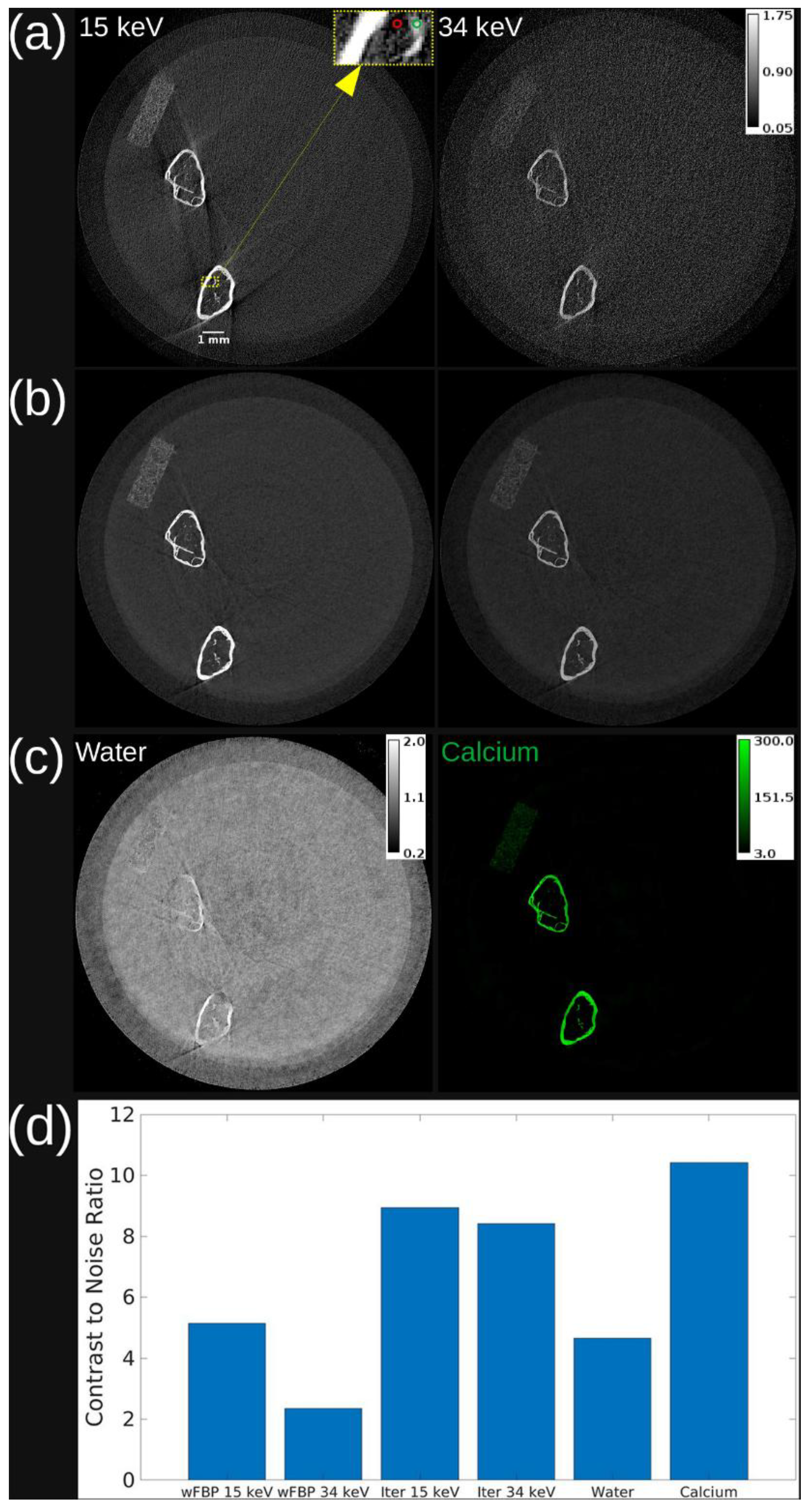
Figure 5.
Violin plots showing differences in BV/TV by genotype. (a) Plot of observed BV/TV values versus APOE genotype. (b) Residuals of confounding variables GLM with formula BV/TV ~ Age + Sex + HN + Age:Sex + Age:HN + Sex:HN versus APOE genotype. The bar with asterisk indicates a significant difference (p<0.05) between APOE44 and the reference genotype level APOE33.
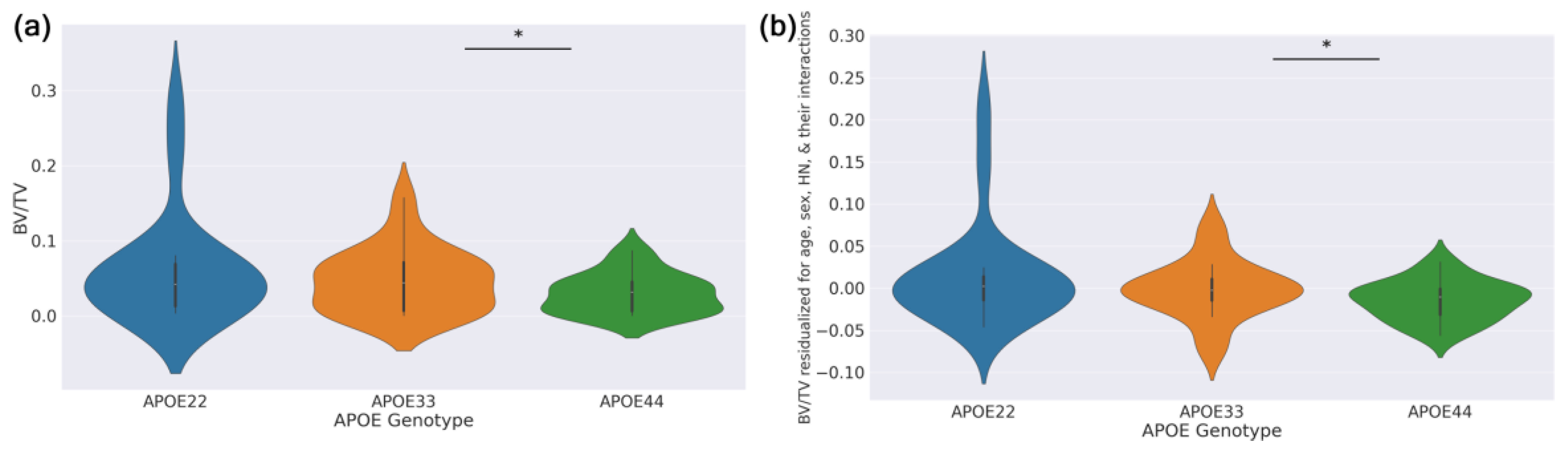
Figure 6.
Violin plots corresponding to Mann-Whitney U comparisons by sex within HN and non-HN subgroups. Bars with an asterisk indicate statistically significant difference (p<0.05) by sex after BH FDR correction. Only femur features with significant sex difference in at least one subgroup have been plotted.
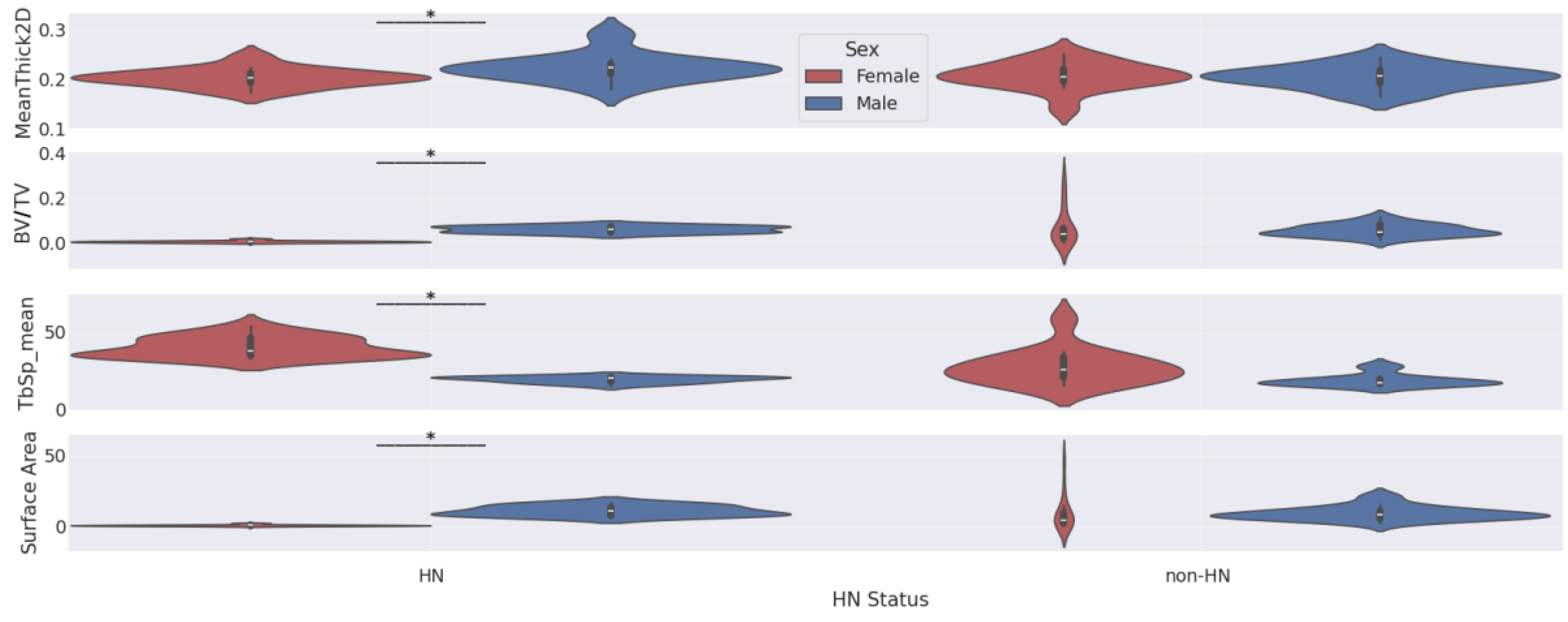
Figure 7.
Violin plots corresponding to Mann-Whitney U comparisons by HN status within female and male subgroups. Bars with an asterisk indicate statistically significant difference (p<0.05) by HN status after BH FDR correction. Only femur features with significant difference by HN status in at least one subgroup have been plotted.
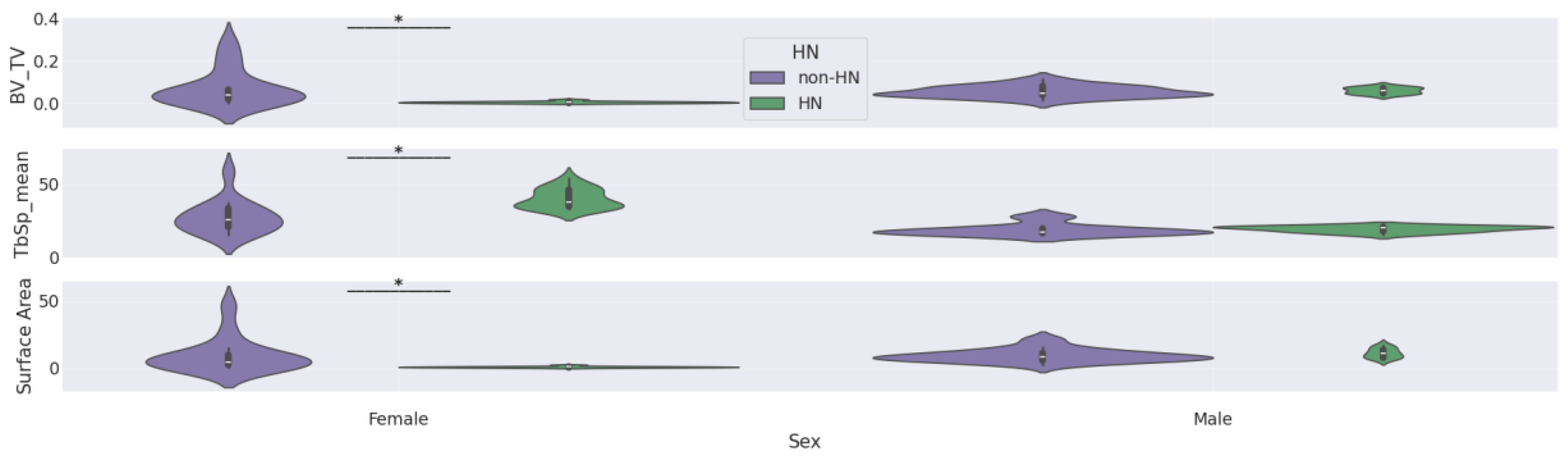
Figure 8.
Scatter plots of femur feature vs. age. Linear regression plots with age as the independent variable, separate linear fits by sex, and (a) MeanThick2D, (b) MeanThick3D, and (c) log(TbSp_mean) as the dependent variable. Each plot includes best fit lines as well as their r2 values, 95% confidence intervals, and p-values (in legend). For brevity, only plots with a statistically significant regression line (p<0.05) in at least one subgroup are shown.
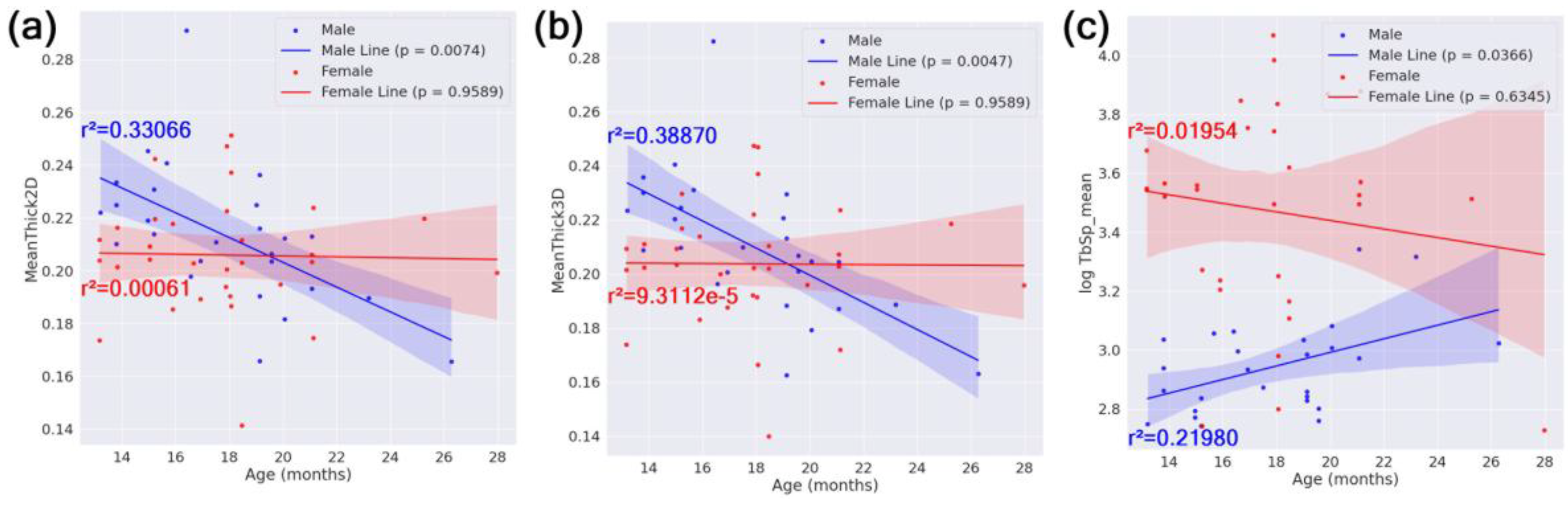
Figure 9.
Qualitative assessment of trabecular bone in metaphyseal region. (a) 3D renderings of combined trabecular and cortical masks from metaphyseal volumes of interest, with example bones from two mice shown for each combination of genotype, HN status, and sex. Heatmaps indicating (b) bone volume fraction and (c) age (in months) for each individual mouse whose bone is displayed in the 3D rendering plot in (a).
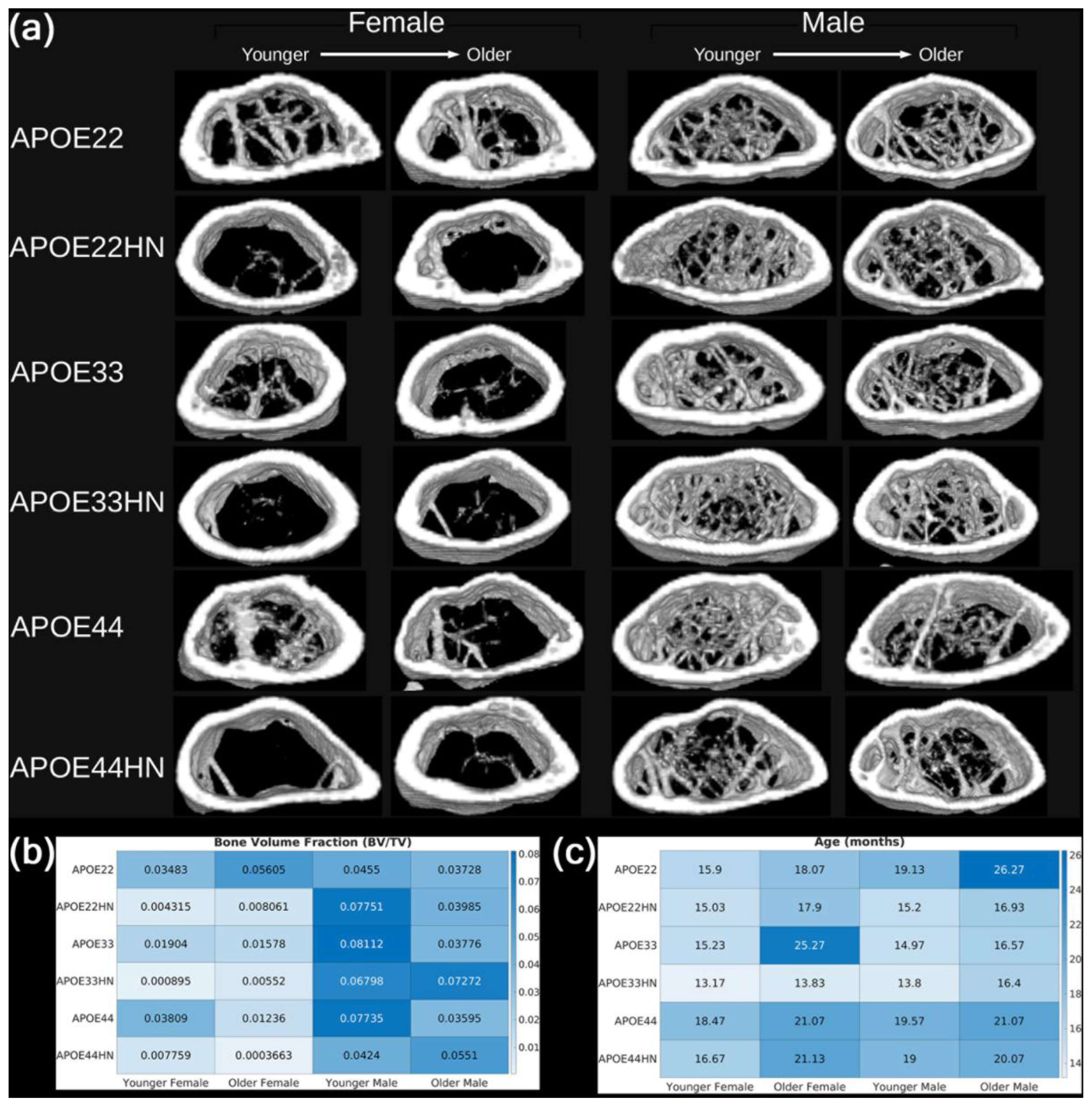
Table 1.
Distribution of mice in femur study by genotype/HN status and sex.
| Genotype | Female | Male | Total |
|---|---|---|---|
| APOE22 | 5 | 5 | 10 |
| APOE33 | 5 | 5 | 10 |
| APOE44 | 5 | 5 | 10 |
| APOE22HN | 6 | 3 | 9 |
| APOE33HN | 5 | 5 | 10 |
| APOE44HN | 5 | 3 | 8 |
| Total | 31 | 26 | 57 |
Table 2.
Age distribution for entire mouse population and for subgroups by genotype/HN status and sex.
Table 2.
Age distribution for entire mouse population and for subgroups by genotype/HN status and sex.
| Group (# of mice) | Age in Months (Mean + Std Dev) |
|---|---|
| APOE22 (10) | 18.88 + 2.88 |
| APOE33 (10) | 18.45 + 5.12 |
| APOE44 (10) | 19.63 + 1.37 |
| APOE22HN (9) | 16.45 + 1.32 |
| APOE33HN (10) | 14.06 + 1.09 |
| APOE44HN (8) | 19.5 + 1.54 |
| Female (31) | 17.74 + 3.38 |
| Male (26) | 17.86 + 3.19 |
| All Mice (57) | 17.79 + 3.27 |
Table 3.
Summary of significant predictors from GLMs.
| Femur Feature | Predictor | Coefficient | BH FDR Corrected p-value | Interpretation |
|---|---|---|---|---|
| BV/TV | Genotype[T.APOE44] | 9.08937 | 0.00976 | APOE44 has a significant positive effect on log(BV/TV) relative to APOE33. |
| BV/TV | Sex[T.Female]:HN[T.HN] | -2.85595 | <1e-5 | The combination of female sex and HN expression has a significant negative effect on log(BV/TV). |
| BV/TV | Age:Genotype[T.APOE44] | -0.484397 | 0.00518 | The change in log(BV/TV) per 1 month increase in age is significantly more negative (i.e., more age-dependent decline) in the APOE44 group than in the APOE33 group. |
| Surface Area | Sex[T.Female]:HN[T.HN] | -2.19199 | <1e-5 | The combination of female sex and HN expression has a significant negative effect on log(Surface Area). |
Table 4.
Summary of significant predictors from stratified subgroup analyses investigating sex and HN interactions. All p-values were computed using Mann-Whitney U tests followed by BH FDR correction.
Table 4.
Summary of significant predictors from stratified subgroup analyses investigating sex and HN interactions. All p-values were computed using Mann-Whitney U tests followed by BH FDR correction.
| Femur Feature | Predictor | Subgroup | BH FDR Corrected p-value | Interpretation |
|---|---|---|---|---|
| MeanThick2D | Sex | HN | 0.03339 | Significant difference in MeanThick2D between female HN mice and male HN mice. |
| BV/TV | Sex | HN | 3.6770e-05 | Significant difference in BV/TV between female HN mice and male HN mice. |
| TbSp_mean | Sex | HN | 3.6770e-05 | Significant difference in TbSp_mean between female HN mice and male HN mice. |
| Surface Area | Sex | HN | 3.6770e-05 | Significant difference in surface area between female HN mice and male HN mice. |
| BV/TV | HN | Female | 0.00050 | Significant difference in BV/TV between female HN mice and female non-HN mice. |
| TbSp_mean | HN | Female | 0.00060 | Significant difference in TbSp_mean between female HN mice and female non-HN mice. |
| Surface Area | HN | Female | 0.00060 | Significant difference in surface area between female HN mice and female non-HN mice. |
Table 5.
P-values after BH FDR correction from Mann-Whitney U comparisons by HN status within genotype by sex subgroups. P-values below the 5% significance level are indicated in bold text.
Table 5.
P-values after BH FDR correction from Mann-Whitney U comparisons by HN status within genotype by sex subgroups. P-values below the 5% significance level are indicated in bold text.
| APOE22 Female | APOE22 Male | APOE33 Female | APOE33 Male | APOE44 Female | APOE44 Male | |
| BV/TV | 0.00433 | 0.78571 | 0.09524 | 0.84127 | 0.02381 | 0.78571 |
| TbSp_mean | 0.00433 | 0.58929 | 0.15079 | 0.46429 | 0.02381 | 0.75000 |
| Surface Area | 0.00433 | 0.58929 | 0.15079 | 0.46429 | 0.05556 | 0.78571 |
Disclaimer/Publisher’s Note: The statements, opinions and data contained in all publications are solely those of the individual author(s) and contributor(s) and not of MDPI and/or the editor(s). MDPI and/or the editor(s) disclaim responsibility for any injury to people or property resulting from any ideas, methods, instructions or products referred to in the content. |
© 2025 by the authors. Licensee MDPI, Basel, Switzerland. This article is an open access article distributed under the terms and conditions of the Creative Commons Attribution (CC BY) license (http://creativecommons.org/licenses/by/4.0/).
Copyright: This open access article is published under a Creative Commons CC BY 4.0 license, which permit the free download, distribution, and reuse, provided that the author and preprint are cited in any reuse.


