
Submitted:
10 September 2025
Posted:
11 September 2025
You are already at the latest version
Abstract
The object of this study is a low-temperature refrigerating machine operating on the auto-cascade cycle and capable of producing cold at two temperature levels simultaneously in a wide range of temperatures down to -195oC. A multi-component zeotropic mixture of refrigerants is used as the working fluid. A hermetic lubricated compressor, one phase separator, a triple-section internal recuperative heat exchanger and two evaporators make the main components of the refrigerator. Sophisticated correlations between the operating parameters of the refrigerator were revealed when analyzing the basic principles of the machine operation. A comprehensive procedure of the auto-cascade cycle thermodynamic calculations considering peculiarities of the working fluid flow transformations through the loop was developed and reported. Building upon this procedure, an algorithm and computer program of full-scale numerical calculations to determine optimal values of such parameters as the working mixture component concentrations, operating temperatures and pressures considering the machine thermodynamic efficiency as a criterion function was implemented. To demonstrate the program operability and potentials the design calculations of the refrigerator operating at the temperature level of -150 oC were conducted and reported. The analysis of the results of calculations confirmed validity and particular relevance of the proposed approach implying the full-scale optimization of the system operating parameters.
Keywords:
Cryogenics
; Thermodynamic efficiency
; Multi-parameter optimization
; Auto-cascade Kleemenko refrigeration cycle
; Zeotropic refrigerant mixtures
; Recuperative heat exchanger
; Phase separator
1. Introduction
At present time, the auto-cascade low-temperature refrigeration cycle (also frequently referred to as the Kleemenko cycle) is rather well known, although it may be an over-statement to tell that it has been expanded broadly in its application. A number of research publications available provide some information on separate and often fragmented results of experimental investigations of such machines [1], theoretical analysis of the system overall designs and some individual components [2,3,4], description of thermodynamic methods to calculate individual components of the cycle (sections of the internal recuperative heat exchanger, a mixing position of forward and return flows of refrigerants) [5,6], etc. However, a comprehensive integrative methodology useful in the design and optimization of such refrigerating machines operating parameters can hardly been observed in those papers. The lack of such a methodology could be one of the reasons for a relatively modest share of the auto-cascade systems on the market of low-temperature medium-sized (cooling capacity) refrigerators (unfortunately, the converse is also the case).
The challenges of developing such a methodology (to design a refrigerator operating by the auto-cascade cycle) could arise with respect to comparatively sophisticated arrangement of the cycle/machine units on the one hand and to peculiarities of thermodynamic description of the working agent (a multicomponent zeotropic mixture of refrigerants) behavior in those units on the other hand. To confirm the words about the design complexity of refrigerators operating by the auto-cascade cycle (ACC) a classical schematic by W. Podbielniak [7] with a cascade of phase separators is presented in Figure 1 and a more contemporary schematic where a rectifying column is applied as an alternative to the phase separator – in Figure 2. Clearly, the use of a rectifying column or a cascade of phase separators would unduly complicate thermodynamic calculations of an individual auto-cascade cycle, let alone calculations of the cycle optimal parameters: the working mixture component concentrations; operating pressure and temperatures implying multiple recalculations of the cycle.
Such a sophisticated arranging of the ACC in which a number of phase separators or a rectifying column are used seems as a consistent and appropriate one in the case where the ACC is applied to the problem of gas separation as A.P. Kleemenko initially suggested [8]. However, such a “cascade” constellation of the cycle is frequently extended to designs of low-temperature refrigerating machines operating on the ACC. The additional complexity of the refrigerating machine introduced by the cascade of phase separators or even a modified rectifying column with a special oil stripping line is justified by a strong necessity to prevent the compressor oil from entering into the low-temperature sections of the refrigerator where temperature of the working mixture flow drops well below the temperature of oil crystallization [3,4].
There is another current view on a feasible arrangement of the units in the auto-cascade cycle and the purpose of a phase separator in a low-temperature auto-cascade refrigerating machine (ACRM). As emphasized in [1], the main task of the phase separator in the refrigerating ACC is to control the component concentrations in the working mixture flow making for a low-temperature side of the refrigerator. The separation of the refrigerant flow into two flows where one is enriched with the lower- and another with higher boiling mixture components enables the temperature, heat and power performances of a ACRM to be considerably improved as compared to the relatively less sophisticated Linde-Hampson mixed-refrigerant cycle.
A flow chart of a low-temperature refrigerating machine (LTRM) operating on the ACC with the only one phase separator, two evaporators and a triple-section internal recuperative heat exchanger (RHEX) is depicted in Figure 3. That schematic is similar to the schematic successfully applied for cooling at the temperature levels down to (-190 ... -195)°С [1]. The usage of the only one phase separator and a lack of any specific oil traps do not result in the compressor’s oil freezing in the low-temperature units of the machine. The authors [1] explained that effect with an appropriate selection of the working mixture (WM) components.
The employment of the only one phase separator in the ACC makes it possible to develop a calculation procedure of a particular ACC. By this is meant the comprehensive thermodynamic calculations of the cycle operating parameters for the given set of input data: the working mixture comprised of Nmix components; concentrations of the components (Ci , i ∈ [1 .. Nmix]); designed temperatures (Tamb, ToH, ToL see Figure 3) and operating pressures (Ps, Pd). As an integral part of the calculations, the optimal temperature of the WM flow separation (T4 see Figure 3); the optimal temperature T13 of the return flow at the RHEX section X outlet port where it is merged with another return flow 8 and the thermal and power parameters of the cycle to be determine. Feasibility of the calculated temperatures at the REHX’s sections inlet and outlet ports should be verified through a procedure of T-Q diagram analysis (also referred to as temperature profiles along the RHEX analysis) as well.
The availability of such a program of the particular ACC thermodynamic calculations enables developing of a more advanced algorithm of full-scale optimization computations of the ACC. The composition (should not be confused with the concentrations) of the WM of Nmix components, the heat loads (QoH, QoL Figure 3) and the temperature levels (ToH, ToL) are the input parameters. Optimal values of the concentrations Ci , i ∈ [1 .. Nmix] of the WM components, operating pressures (Ps, Pd), temperatures of the phase separation T4 and mixing/merging T13 to be determine in the course of those full-scale calculations. A minimal value of the compressor input power could be accepted as an optimality criterion.
The above-mentioned problem of calculating thermodynamic and transport properties of multicomponent zeotropic mixtures of refrigerants can be solved by implicating the numerical procedures provided by NIST Standard Reference Database 23, v.9 [9] and Database 4, v.3.2 (hydrocarbon mixtures database - SUPERTRAPP) [10] into the program of the ACC optimization calculations.
To gain an insight into the difficulties emerging in the course of developing the computational design procedure of a LTRM operating on the ACC and to distinguish clearly between the given (input) parameters of the ACC and parameters to be optimized through the calculations, let us remind briefly the main principles of the auto-cascade cycle operation.
2. Operating Principles of the LTRM Running on the ACC
As mentioned above the schematic of the LTRM operating on the ACC (Figure 3) was successfully applied in developing and full-scale testing of 6 micro coolers [1] and seems to work as well in theoretical analysis of the cycle and some design guidelines.
The hermetic lubricated compressor I (Figure 3) inhausts the WM flow at state 1 as super-heated vapors at the temperature Т1 and pressure Ps; the mass rate of the flow 1 is m; the mixture component concentrations are consistent with the charging (design) concentrations of the WM of Nmix components: Ci , i ∈ [1 .. Nmix], where Nmix ∈ [3 … 5]. The compressor boosts the WM pressure up to the value of Pd while the mixture temperature goes from Т1 up to Т2 (state 2). In the after-cooler III the mixture is cooling down to the temperature T3 = Tamb + ∆Т3 in the process of heat exchange with ambient air. A partial condensation of the WM flow at the after-cooler outlet (state 3) is possible but not required. The filter-dryer IV is designed for eliminating potential residual water vapors in the refrigerant flow.
In the high temperature section XII of the RHEX the working zeotropic mixture forward flow 3→4 is being gradually cooled and partially condensed at the variable temperature (T3 … T4) while in heat exchange with the cooler return flow 15→1 of the mixture. A fraction of the liquid phase in the forward flow goes up and the flow’s quality goes down from x3 to x4, respectively. The two-phase flow of the refrigerant at the temperature T4 and pressure Pd enters the phase separator V.
In the phase separator V the two-phase flow 4 is split into two flows: of saturated vapor 5 and liquid 6 phases of the WM. The saturated vapor flow 5 at the temperature T5 = T4 and pressure Pd is enriched with the lower boiling (with lower value of TNB) components of the mixture and their concentrations CiV , i ∈ [1 .. Nmix] are significantly different from the mixture charging concentrations. The mass rate of the vapor flow 5: mV = m⋅x4. The saturated liquid flow 6 at the temperature T6 = T4 and pressure Pd is enriched with the less volatile (with higher values of TNB) mixture components of concentrations: CiF , i ∈ [1 .. Nmix]. The mass rate of the liquid flow 6: mF = m⋅(1 - x4).
The p-h diagram of the ACC is depicted in Figure 4. The ACC p-h diagram is comprised of three interdependent diagrams (Figure 4 A, B and C) as it follows from the mixture component concentrations variations while the mixture is circulating through the loop. The saturation lines, all the thermodynamic curves and processes in the p-h diagram in Figure 4 are corresponding with the results of the actual thermodynamic calculations of the LTRM on the ACC using the RefProp 9.0 (NIST standard reference database 23) computational procedures.
The flow 6 of the saturated liquid goes through the throttle capillary VI to lower the value of the flow pressure down to Ps and then enters the optional high temperature evaporator VII where the liquid phase is evaporated partially due to the actual heat load QoH. Upon leaving the evaporator VII, the refrigerant flow 8 with the following parameters: T8 = ToH - ∆Т8 (or T8 =T7 in the case that the evaporator VII is not presented in the LTRM); Ps; mF = m⋅(1 - x4) and CiF , i ∈ [1 .. Nmix] is mixed with the return flow 13 of the refrigerant and then directed into the middle section XI of the RHEX (state 14).
Upon leaving the phase separator V the flow 5 of saturated vapor goes through the RHEX sections XI and X sequentially while cooling with the refrigerant return flow 12→15. In the process the working mixture components in the forward flow 5→10 turns completely (or partially) into the liquid state. After the throttle capillary VIII the working mixture flow 11 with the following parameters: temperature T11 < T12; Ps; concentrations CiV , i ∈ [1 .. Nmix] and mass rate m⋅(1 - x4) enters the low temperature evaporator IX where it starts to boil and being partially evaporated due to the actual heat load QoL. Meanwhile the temperature of the flow 11→12 is not invariable but goes up from T11 to T12 = ToL - ∆Т12. Then the flow is directed into the low temperature section X of the RHEX.
At the outlet of the low temperature section X of the RHEX the return flow of the refrigerant with parameters corresponding to the state 13 is mixed with the return flow 8 leaving the high temperature evaporator VII. As a consequence of the process of the flows 13 and 8 merging the flow 14 is developed with the following parameters: T14; Ps; the component concentrations once again are corresponding with the charging ones Ci , i ∈ [1 .. Nmix] and the mass rate is back to its value before the flow separating: m = m⋅ x4+m⋅(1 - x4).
3. The Procedure of the ACC Thermodynamic Calculation
The presented brief description of the processes taking place in the loop of a low-temperature auto-cascade refrigerating machine offers a clearer view of peculiarities of thermodynamic computations of the cycle. Unlike to the classical vapor-compression refrigeration cycle operating on a pure substance or to the Linde-Hampson mixed refrigerant cycle the thermodynamic computations of the ACC cannot be reduced to ”one-shot” calculations of the thermodynamic properties of the working mixture at the given cycle states for a number of reasons reported below.
Under the given charging concentrations of all Nmix components of the WM: Ci , i ∈ [1 .. Nmix]; operating pressures: (Ps, Pd); the temperatures of cooling and actual heat loads (the cooling capacities): (T12, QoL), (T8, QoH), a specific value of the temperature of separation T4 is still unknown a priori, even if we are aware that it lies somewhere within the interval of [Tamb … T12[. Determination of the optimal value of T4 requires a particular optimization procedure involving multiple computations of the ACC. As this takes place, a minimal value of the compressor input power could be accepted as an optimality criterion.
A specific value of the temperature Т13 of the refrigerant return flow 12→13 at the RHEX low-temperature section X outlet is unknown in advance as well and requires its own independent procedure of calculations. The target value of Т13 lies within the limits of ]T12 … T5[ and it should ensure the irreversibility of the process of flows merging to be at a minimum. In other words, a value of the entropy generated in the process of merging ΔSgen should tend to its minimum:
In case of the ACC the working mixture of refrigerants goes through the phase transitions both in the forward 3→10 and in return 12→1 flows in all three sections of the RHEX. The WM temperature changings in each of the flows throughout the RHEX may run over 100 … 150 degrees. Under such circumstances, it could lead to a serious mistake to appoint in advance a value of the minimal temperature difference ∆ТoutRHEX to one of the RHEX sides (either to the cold side: ∆Т10_12 = T10 - T12 = ∆ТoutRHEX or to the hot side: ∆Т1_3 = T3 - T1 = ∆ТoutRHEX) as it is ordinarily being done in a classic case of the vapor-compression refrigeration cycle operating with a pure refrigerant or was done with the ACC thermodynamic calculations [6]. In case of a mixed refrigerant LTRM (operating on either the ACC or the Linde-Hampson) an additional procedure to analyze heat capacity rates of both forward and return refrigerant flows is demanded. As a result of that analysis the RHEX side with the minimal temperature difference ∆ТoutRHEX between the flows will be determined.
The preceding reasoning also means that implementation of the first law of thermodynamics for the RHEX (the condition of the general heat balance of the flows) is necessary but not sufficient for the ACC case. The well-known procedure of a heat exchanger T-Q diagram analysis (also referred to as temperature profiles along the heat exchanger with transferred heat) is required for every cycle calculation. The results of the ACC thermodynamic calculations may be considered as valid only when the T-Q diagram of the RHEX has demonstrated its feasibility.
Let us outline the procedure of thermodynamic calculations of the ACC for the case when a value of the temperature of the WM separation Т4 is already specified.
3.1. Thermodynamic Calculations of the ACC Under Given Value of the Temperature of Separation
- Given/Input data:
Working mixture: components of the mixture in a number of Nmix; the charging concentrations of the components Ci , i ∈ [1 .. Nmix].
Operating pressures: either Ps and Pd or Ps and a value of the pressure ratio ψ = Pd / Ps ;
Temperature parameters: the temperatures of the objects of cooling: ToL and ToH; the ambient temperature Тamb; the temperature of the working mixture separation Т4; the temperature differences at the ACC heat exchangers outlets: ∆Т3 = T3 - Tamb; ∆Т8 = ToH - T8; ∆Т12 = ToL - T12 and ∆ТoutRHEX (the minimum acceptable temperature difference between the forward and return flows at the RHEX outlet to be appointed after the analysis of heat capacity rates of the flows).
Heat parameters: values of the actual heat loads on the evaporators: QoL and QoH.
- Results of calculations:
the thermodynamic parameters of the WM in all the states of the ACC (see Figure 3 and 4), the compressor power parameters, the heat exchangers heat loads.
- Procedure of calculations
3.1.1. The Calculation of Thermodynamic Parameters of the WM Flows at the RHEX’s Section XII Outlet 4 and the Phase Separator V Outlets 5 and 6 (see Figure 3)
A thermodynamic equation of state f (actually, a set of numerical subroutines written in the FORTRAN programming language) developed by NIST: Standard Reference Database 23, v.9 [9] and Database 4, v.3.2 (hydrocarbon mixtures database - SUPERTRAPP) [10] is utilized for calculations of zeotropic mixtures of refrigerants thermodynamic and transport properties.
The values of enthalpy, quality, and concentrations of the WM flow 4 at the phase separator inlet are calculated by the mentioned equation of state f taking a temperature, pressure and the WM component concentrations as input data:
The enthalpy of the saturated vapor flow 5 at the phase separator outlet:
The enthalpy of the saturated liquid flow 6 at the phase separator outlet:
The mass rate m of the WM flow at the separator inlet 4 is linked to the mass rates of the liquid mF (flow 6) and vapor mV (flow 5) phases by the following equation:
3.1.2. Temperature and Quality of the Two-Phase WM Flow 7 After the High-Temperature Capillary Tube VI Is as Follows:
Assuming the high-temperature evaporator VII is presented in the cycle, then the fulfillment of the following condition to be verified:
where. In the event that the condition Eq. (7) is false, then the ACC ongoing calculation should be terminated and the current set of input data considered as unsuitable for the required temperatures of cooling.
Assuming the high temperature evaporator VII is not presented in the cycle, then the condition Eq. (7) to be ignored.
The given actual heat load QoH on the high-temperature evaporator determines the calculated value of the refrigerant mass rate mH in the ACC to be in line with a value of QoH:
3.1.3. The Refrigerant Flow 8 at the High-Temperature Evaporator VII Outlet
The enthalpy and entropy of the two-phase flow 8:
while for the ACC schematic including the high-temperature evaporator and when that evaporator is skipped.
3.1.4. The Calculation of Thermodynamic Parameters of the Forward 10 and Return 1 Flows at the RHEX’s Outlets
The thermodynamic parameters of the WM flow at the RHEX’s outlets 3 and 12 are calculated plainly since the temperatures, pressures and the mixture component concentrations are known in advance:
Since the temperatures of the refrigerants flows at the RHE’s outlets 10 and 1 are indeterminate, then the following two-step procedure should be applied.
The calculations of the temperatures and enthalpies of the flows at the RHEX’s outlets 10 and 1 at first approach.
The temperatures of the refrigerant flows at the outlets 10 and 1 will be calculated to a first approximation using the given values of the RHEX outlet minimum acceptable temperature difference between the forward and return flows ∆ТoutRHEX:
In that case the values of enthalpies at the RHEX’s outlets 10 and 1:
The specific heat contents of the forward 3→10 and return 12→1 flows of refrigerant:
To calculate the ultimate values of Т1 and Т10, then the analysis of the flows’ specific heat content ratio to be performed by using the NTU (or effectiveness) method [11].
In the event that ∆h3_10 ≥ ∆h12_1, the temperature Т1 should keep its value from the first approach calculation Eq.(13). At that time the refrigerant flow enthalpy at the RHEX’s outlet 10 to be calculated from the RHEX general heat balance equation:
The ultimate value of the refrigerant flow 10 temperature at the RHEX outlet:
In the event that ∆h3_10 < ∆h12_1, the same procedure will be applied to the opposite side of the RHEX. This time the temperature Т10 should keep its value from the first approach calculation Eq.(12) and the refrigerant flow enthalpy at the RHEX’s outlet 1 to be calculated from the general heat balance:
The ultimate value of the refrigerant flow 1 temperature at the RHEX outlet:
Redundant testing of the refrigerant flow 1 phase state.
Once the low pressure refrigerant flow at the RHEX’s outlet 1 is still in a two-phase state (and such an outcome can have a small, but non-zero probability):
and its temperature is close to the ambient temperature:
then a threat of the liquid phase penetration into the compressor arises. This operating mode of the LTRM is considered as inadmissible one and further calculations of the cycle with the given input parameters should be terminated.
In case that the refrigerant flow 1 at the RHEX outlet is still in a two-phase state (x1 < 1) but its temperature T1 < (Tamb +∆Т3), then the calculations to be proceed. As this takes place, a supplementary heat exchanger should be provided between the RHEX and compressor (not shown in Figure 3) and considered in the algorithm of the LTRM calculations. The two-phase refrigerant flow 1 of low-pressure Ps has to be heated up in that heat exchanger in a process of heat exchange with ambient air to the temperature T1 = Tamb - ∆Т3 where it turns into a state of saturated (or overheated) vapors.
3.1.5. Calculations of the Refrigerant Flow Thermodynamic Properties at State 11 (Figure 3)
After the RHEX’s section X the WM flow 10 of high pressure Pd enters the capillary tube VIII, where it is throttled down to the pressure Ps. The flow temperature at the capillary tube outlet – the low-temperature evaporator IX inlet is as follows:
The low-temperature evaporator (and the current calculating mode of the LTRM as a whole) can be considered as an admissible one only providing the condition:
where . In case of the condition Eq.(23) failure, the ACC calculations should be terminated and the current set of input data considered as an unsuitable one for the required temperatures of cooling.
The value of the refrigerant mass rate mL that balances the actual heat load QoL on the low temperature evaporator:
In the ACC schematics with two evaporators (both high- and low-temperature) operating concurrently the larger of mL and mH values should be considered for the value of mass rate of the refrigerant running through the compressor:
An excessive cooling capacity in any of two evaporators (where the value of calculated mass rate is lower than the accepted one Eq.(25)) is inevitable. This is an immanent shortcoming of the ACC with two evaporators (the case when both evaporators have the same calculated mass rate is extremely unlikely).
For the LTRM operating on ACC with the only one (low-temperature) evaporator, the mass rate of the refrigerant is as follows:
3.1.6. Calculations of an Optimal Value of the Return Flow 13 Temperature at the Outlet of the RHEX Low-Temperature Section X
Direct calculations of the temperature of the return flow at state 13 (Figure 3) cannot be made by using only equations of heat exchange in the RHEX for an intricate interdependency of the temperatures Т9, Т13 and Т14. The value of temperature Т14 is not governed just by the processes of heat exchange in the RHEX’s section X (that means Т14 ≠ Т13) but by the process of merging of the return flows 13 and 8 as well. Since the concentrations of the WM components in flows 13 and 8 are substantially different therefore a simple decision of Т13 = Т8 is unacceptable as it does not take into consideration the heat of the substances mixing.
The process of merging of the refrigerant flows 13 and 8 may be assumed as an efficient one when irreversible losses of the process tend to the minimum. The minimal value of the entropy ΔSgen generated in that mixing-merging process (see Eq.(1)) can be accepted as a criterion of irreversibility. The expression for specific entropy changing in the process of the refrigerant flows 13 and 8 merging is as follows:
The specific value of entropy at the state 14 can be calculated with the value of enthalpy h14 which in turn is defined from the following equation:
In a calculation procedure a value of Т13 from the range of Т13 ∈ [Т12 ... Т1] (see Figure 5) that corresponds to the minimum value of entropy generation ∆sgen Eq. (27) should be determined. As it can be seen from the Figure 5, the minimal value of the temperature difference (Т14 – Т13) between the flows 14 and 13 corresponds with the minimal value of the generated entropy ∆sgen that was to be quite expected.
Considering that the criterion function ∆sgen (Т13) is not a smooth function in the general case, therefore it is reasonable to calculate the minimal value of ∆sgen using the methods of golden section or interval bisection. The outcome of the procedure is the specific values of the temperatures Т13 (Eq. (27), (28)) and Т14 :
3.1.7. Procedure of the T-Q Diagram (the Temperature Profiles of the Refrigerant Forward and Return Flows in the RHEX) Calculations
The temperatures Т1 and Т10 of the WM flows at the corresponding RHEX’s outlets (see p. 3.1.4.2) are calculated based on the already mentioned following assumption. The given value of the minimal temperature difference ∆ТoutRHEX, which has to be set at one of the RHEX’s sides, is invariable for all calculating modes. In other words, the effectiveness ε [13] of the counterflow RHEX’s sections X-XII is assumed to be invariable regardless of the input data for the ACC calculations (the component concentrations, pressure, temperature of separation, etc.). Such an approach is well known and widely applied in cryogenics. A significant imperfection of that method lays in the fact that fulfillment of the first law of thermodynamic for the RHEX (the heat balances of the flows Eq. (18), (20)) does not guarantee the heat exchanger’s operability [1,12]. Some extra calculations and subsequent T-Q diagram (the temperature profiles of the forward and return refrigerant flows, see Figure 6) analysis are strongly demanded. In the event that the temperature difference between the forward (hot) Тhot and return (cold) Тcold flows of the refrigerant in every cross section of the RHEX is not lower than a preset value of ∆ТminRHEX : (Тhot - Тcold) ≥ ∆ТminRHEX, the heat exchanger should be considered as an operable one for the set of given input parameters. An operative T-Q diagram embracing all three sections of the RHEX of a LTRM operating on the ACC is presented in Figure 6. Having the heat balances of the refrigerant flow in the RHEX written in terms of specific enthalpies (see Eq. (16), (17)), then the specific heat transferred from the forward to return flow of the refrigerant is used as an abscissa in the T-Q diagrams in Figure 6 and Figure 7.
Once in any cross section of the RHEX the temperature difference between the flows occurs lower than the preset minimal value: (Тhot - Тcold) < ∆ТminRHEX (see Figure 7), then it would mean that the given value of the minimal temperature difference ∆ТoutRHEX set at one of the RHEX’s sides is unattainable for the considering input parameters and the current calculating mode is unrealizable. Within the framework of the reported procedure of the ACC thermodynamic calculations an on-line (”on-the-fly”) tailoring of the value of ∆ТoutRHEX or another procedure to calculate directly the values of the outlet temperatures Т1 and Т10 as the cycle calculations advance are not provided.
The procedure of T-Q diagrams calculations is well known and has been reported many times [6,12]. As a peculiarity of the RHEX T-Q diagram calculation for the ACC it should be noticed a discontinuous change of the WM component concentrations and mass rate both in the forward flow 4 → 5 (Figure 3): Ci → CiV; m → m⋅x4 and in the return flow of the refrigerant 13 → 14: CiV → Ci; m⋅x4 → m.
A calculation grid for the T-Q diagram is built up in such a way that the specific states 4, 5, 13 and 14 of the refrigerant flow were located right in the grid nodes. To simplify the task, the calculation of T-Q diagram can be performed in parts: for the RHEX’s sections X and XI combined together and separately for the section XII.
Both the RHEX operability checking and the calculated values of the intermediate temperatures Т9 and Т15 (see Figure 6) of the forward and return flows of refrigerant are the results of the T-Q diagram calculations, which are strongly required for some subsequent design calculations of the heat exchanger sections.
3.1.8. The Calculation of the Working Mixture Compression in a Reciprocating Hermetic Lubricated Compressor
The input power Winp of the compressor can be calculated as follows:
where, Wis is the isentropic work of the compressor; Wfr is friction losses; ηm is the efficiency of the compressor’s electric motor (a specified parameter) and ηc is the efficiency of the compressor.
The isentropic work of the compressor:
where T1’ = T1 + ΔTc, sup is the temperature of the refrigerant vapor flow sucked into the compressor (state 1, Figure 3) and super-heated by the compressor’s electric motor (state 1′); ΔTc, sup is the suction line superheat; s2,is = s1’ (T1’, Ps, Ci) is the value of a specific entropy of isentropic compression.
A semiempirical formula is used to calculate the friction losses:
where n – a coefficient for the compressor dead space volume; k – a polytropic exponent; α and β are empirical coefficients reflecting influence of the temperature of condensation (in case of the ACC the temperature Т3 is accepted) and superheating of the vapor in the compressor cylinder as a function of a specific compressor type (in our case hermetic, open-type, vertical, compressor sizing, etc.) and a refrigerant; Pfr is the pressure of friction.
The efficiency of the compressor ηc Eq.(30) is evaluated from the following empirical equation [14]:
where b is the empirical coefficient reflecting influence of a refrigerant temperature of evaporation (in case of the ACC the WM flow temperature at the evaporator’s outlet port Т12 is accepted).
Internal superheating ΔTc, sup (see Eq. (31)) caused by the compressor’s electric motor:
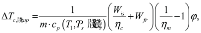 where cp (T1, Ps, Ci) is the specific heat of the vapor flow; ϕ is an empirical coefficient. Having Wis as a function of ΔTc, sup Eq. (31), which in turn is dependent upon Wis Eq. (34), then an iteration procedure is demanded to calculate all the compressor parameters.
The coefficient of performance of the ACC (in case of only one evaporator):
As with QoL, the СОР should be related with the temperature Т12 of the refrigerant flow at the evaporator outlet (the highest value of the flow temperature in the evaporator). In a case of the ACC with two evaporators (two temperature levels and cooling capacities), a concept of the COP is not applicable to the system at all.
3.2. The Procedure of Calculations of the Optimal Temperature of Separation
Given: the input data for calculating the optimal value of the temperature of separation are essentially the same as in the case of thermodynamic calculations of a particular ACC (see p. 3.1), except that a value of the temperature of separation T4 is not specified.
Instead of the exact value of T4 a range of changing of feasible values of the temperature of separation is specified. In case of the ACC’s schematic with a single low-temperature evaporator that range is as follows:
or for the ACC’s schematic with two evaporators:
The thermodynamic calculations of the ACC are performed through the reported procedure (see p. 3.1) for the values of T4 taken sequentially at the upper, lower range limits Eq. (36) or (37) and at an intermediate value, having a gradual downranging as the procedure objective. The value of the optimal temperature of the WM phase separation is appropriate to a computed mode of the LTRM operating on the ACC with a minimal value of the compressor’s input power Winp (see T4 = 15oС, Figure 8).
As it can be seen from Figure 8, the function Winp (T4) is not a smooth and continuous one. In the process of the ACC thermodynamic calculations difficulties emerge when some T-Q diagrams are found to be inoperable (see T4 = 18 oС, 19oС and <14oС Figure 8), the temperature Т11 ≥ Т12 or the NIST RefProp’s numerical procedures calculating thermodynamic properties of zeotropic mixtures generate some critical errors. Each of these cases mean a discontinuity of the function Winp (T4) and the corresponding operating modes to be excluded as it takes place for T4 = 18 oС and 19oС in Figure 8. The algorithm of the optimal temperature of separation calculations provides those inoperative modes handling.
3.3. The Procedure of Calculations of the Optimal Concentrations of the Working Mixture Components
- Given data.
The WM composition: the names of the mixture components in the given number of Nmix (the charging concentrations Ci of the components are unknown and to be specified in the course of calculations).
The operating pressures, temperature parameters (excluding the temperatures of the WM phase separation) and heat parameters are the same as in the case of thermodynamic calculations of a particular ACC (see p. 3.1)
In the course of the calculations the optimal charging Ci concentrations of the mixture components and the optimal value of the temperature T4 of the WM phase separation providing a minimal value of the compressor’s input power Winp are to be specified.
The procedure of calculations implies two stages. At the first stage (the so-called rapid calculations) a permanent sparse computational grid for concentration of every component of the working mixture is developed. The concentration СiJ of each i ∈ [1 … (Nmix – 1)] independent component is varied along the sparse grid form some preset initial value of Сo in increments of ΔCSP = 0.10, kg/kg under the limiting condition СiJ < 1.00 in any j-node of the grid:
The ACC thermodynamic calculations are conducted by the procedure reported in p. 3.2 for every node on the (Nmix – 1)-multidimensional (the ensemble of Сi, i ∈ [1 … (Nmix – 1)]) sparse computational grid of the component concentrations (see Figure 9А). The calculated modes with inoperable T-Q diagrams are excluded from the subsequent analysis. From all the solutions available on the sparse grid the solution with the minimal value of the compressor’s input power is selected for the following calculations. The concentrations of the WM components corresponding to the best mode detected on the sparse grid is to be used as a starting-point for the further development of a denser computational grid for the subsequent refinement calculations. In the event that there were no solutions found on the sparse computational grid, then the given pair of the operating pressures (Ps, Pd) is considered as an inapplicable one for the given WM composition (mixture components), temperature or thermal parameters of the ACC.
In the second stage of the calculations a search for the global minimum of the function Winp(Сi, T4) on a dense computational grid of concentrations is continuing. A structure of the dense grid is similar to the sparse grid Eq. (38), but with two considerable differences. The first and nonprincipal one is that the dense grid is being built with a smaller value of the increment ΔCdn = 0.01, kg/kg. The second one is that the dense grid is not a fixed but rather a flexible structure to be rebuilt and adjusted from calculation to calculation. A variable and limited range of the WM component concentrations (below the full range of ]0 .. .1[,kg/kg) allows such an adaptation. A temporary local dense grid is being built around a set of some specified concentrations Сi, i ∈ [1..Nmix] taken from the previous calculations (more details below). The very first local dense grid is built around the working mixture concentrations Ci_o obtained from the best solution on the sparse grid.
A widely applied algorithm of the gradient descent is exploited for searching of the global minimum of the target function - Winp(Сi, T4). For a current set of the mixture component concentrations Ci_o the following (Nmix – 1)-dimensional dense computational grid with the increment of ΔCdn to be built:
where (2⋅Nk + 1) is an overall number of the dense grid nodes for the every of (Nmix – 1) component concentrations. The specific value of Nk is picked up from the range of Nk ∈ [2 .. 5] depending on a CPU computing power available. The ACC thermodynamic calculations are conducted in the nodes of a current dense grid by the procedure of calculation of the optimal temperature of separation reported above in p. 3.2.
The results of the ACC calculations in the dense grid nodes are to be analyzed. The calculated mode with the lowest value of Winp(Сi, T4) is selected as the next point on the gradient descent curve (see Figure 9В). This point (actually the set of the mixture component concentrations) is the central node for the next local dense grid Eq. (39) to be built around. Potentially shared nodes of the current and previous local dense grids are under control and repeated calculations of the same modes are excluded. The procedure is reiterated over and over again until the function Winp(Сi, T4) gets into a point of its global minimum.
Occasional calculations of the ACC for an arbitrary set of the mixture component concentrations that lies beyond the current dense calculation grid is provided for reducing a probability of the target function global minimum missing (to a certain extent it is an analogy of mutations in the genetic algorithms of optimization).
Calculations of an optimal value of the temperature of separation Т4 have to be conducted in every node of the dense computational grid (see Figure 9 C). Since the optimal value of Т4 lies within a rather wide range of potential temperatures [-60 … +30] oC its calculation with accuracy of let’s say 1 deg substantially slowing down the rate of the whole optimization procedure.
Calculations of T-Q diagrams for every mode is a CPU-time consuming lasting process as well. However, the procedure of T-Q diagrams operability checking could be postponed for the CPU-time saving as distinct from the calculations of the optimal value of Т4. The ACC thermodynamic calculations both on the sparse and dense computational grids are conducted at first without T-Q diagram calculations and analysis. At this stage of calculations, the calculated modes are considered to be operating and acceptable if they merely meet the given temperature parameters of the cycle. It is precisely these results that are presented in Figure 9B. Once the global minimum of the function Winp(Сi, T4) has been located, the calculations and analysis of T-Q diagram are implemented but in the reverse sequence: from the modes with the lower to higher values of Winp(Сi, T4). The T-Q diagram calculations and analysis are carried out up to the first mode with an operable T-Q diagram. As this takes place, a sizeable number of the calculated modes can be considered as inadmissible (see Figure 9 A, D).
Adopting the input power consuming by a hermetic compressor in the ACC as a criterion function for the cycle optimization calculations the following must be emphasize. In course of the thermodynamic calculations of the ACC operating on different zeotropic mixtures of refrigerants it has been repeatedly noticed that Eq. (30) to calculate the compressor’s input power produces comparatively invalid results. This latter point could be caused through the use of some semiempirical coefficients in Eqs. (32)-(34), which were developed for pure refrigerants rather than multicomponent zeotropic mixtures. Therefore we would recommend applying the compressor’s isentropic work Wis(Сi, T4) as a criterion function in the ACC optimizing thermodynamic calculations where a repeated comparison of the compressor’s work in the ACC different operating modes is taking place. The calculated values of Winp Eq. (30) should rather serve for reference purposes.
3.4. The Procedure of Calculations of the ACC Optimal Operating Pressures
The distinctive feature of zeotropic mixtures of refrigerants used in the ACC as the working fluid is a lack of the unique interdependence between the temperature and pressure in the two-phase envelope (notice the intersections of isobars and isotherms in the two-phase envelopes in Figure 4) as it takes place for pure refrigerants. For this reason the given-input temperature parameters of the ACC (temperatures of the object of cooling ToL and ambience Tamb) do not determine the values of operating discharge Pd and suction Ps pressures in the ACC anymore. The latter means that in case of a LTRM operating on the ACC a special optimization procedure to calculate values of the operating pressures is demanded.
Feasible values of the ACC operating pressures should vary within some ranges that are determined by specifications of the compressors employed in the ACC. Since any leakages in the LTRMs of low and average refrigerating capacities operating on mixed refrigerants are extremely undesirable (not to say inadmissible), then hermetic, lubricated compressors have to be used in these machines [1]. Actual hermetic compressors are capable to keep the following operating and peak/maximum pressures. The maximal admissible discharge pressure for scroll-type compressors is 29.5 bar (abs.) under the maximum operating (steady) pressure of 20 bar (Copeland compressors). For reciprocating hermetic compressors those figures rise up to 28.9 bar and 25.9 bar, respectively [15]. The operating pressures ranges for reciprocating hermetic compressors are as follows: the suction pressure - [1.1 … 13.3], bar; the discharge pressure - [3.1 … 25.9], bar; the maximal value of the compression ratio - (12-13), bar/bar. On the basis of these data, the following computational grid of the operating pressures [Ps × Pd] of an auto-cascade refrigerating machine is developed:
In the reporting thermodynamic calculations of the ACC the following limiting values of the pressures and compression ratio were used:
The searching procedure of the operating pressures optimal values essentially comes down to running over the all available pairs of operating pressures (Ps i, Pd j) on the computational grid [Ps × Pd] Eq. (40) conducting calculations for the every pair to determine the optimal concentrations of the WM components (by the procedure p. 3.3) with subsequent comparative analysis of the compressor’s input powers in different calculations. For the given WM composition, thermal and temperature parameters of the ACC, a pair of pressures (Ps i, Pd j) corresponding with the minimal power consumption of the compressor will be considered as the optimal. The results of the ACC calculations on the computational grid of pressures Eq. (41) are presented in Table 1.
The computational grid of pressures Eq. (40) with parameters Eq. (41) is rather sparse for having just (5 × 11) nods. For this reason, a special procedure of optimization for calculations on the pressure grid was not applied (the method of direct search was used).
4. The Results of the ACC Calculations
The procedure of the ACC full-scale optimization calculations reported in pp. 3.1 - 3.4 was applied for thermodynamic calculations of the mixed refrigerant LTRM with the only one phase separator; one low-temperature evaporator and an internal three-section recuperative heat exchanger (see Figure 3). The three-component mixture (Nmix = 3) of hydrocarbons: butane-ethane-methane was used as a refrigerant. The temperature of ambient air: Tamb = 25oС. The temperature of the object of cooling: ToL = -150oС. The actual heat load on the low-temperature evaporator (the system’s cooling capacity): QoL = 100 W.
The parameters of the computational grid built for the WM component concentrations corresponded to the parameters in Eq. (38)-(39). The increments (steps) of the sparse and dense grids of the concentrations were of: ΔCsp = 0.1, kg/kg and ΔCdn = 0.01, kg/kg, respectively. The extension of the current (temporary) dense grid: Nk = 3 (see Eq. (39)).
The parameters of the computational grid built for the ACC operating pressures corresponded to the parameters in Eq. (40)-(41).
While a computer was running the program of the ACC full-scale thermodynamic calculations, the most telling parameters of the already calculated modes could be monitored: a pair of the current operating pressures (Pd, Ps) with the corresponding values of the component charging concentrations Ci and temperature of separation T4 already optimized for those pressures; the compressor input power Winp; the refrigerant mass rate m and temperature differences at the RHEX’s sides (ΔT3-1, ΔT10-12). In the event that the program failed to find solution for the current pair of operating pressures (it means that either the required condition Т11 < Т12 = (ToL - ∆Т12) failed, or the T-Q diagram was found to be inoperable, or the RefProp’s subroutines generated a critical error, etc.) then an appropriate message was displayed instead of the data.
After completion of the optimization calculations on the computational grid for the pressure, the results of successful modes were sorted according to the values of the compressor input power Winp (see Table 1) from the lower to higher values. The inoperable modes were excluded and not presented in Table 1.
The computing program offers to choose any of the modes presented in the table (on the PC’s screen) and then displays the detailed information on the thermodynamic parameters of the ACC; the compressor’s power characteristics; the system heat exchangers actual heat loads; the T-Q diagram graphical plotting, etc. A detailed data set on the operating parameters of the simulated ACRM is available after the calculations but only of most relevance are displayed. The complete data set including thermodynamic and transport properties of the WM at every state of the ACC (states 1-15, Figure 4), the temperature profiles of the forward and return flows in the RHEX, etc. are output at the same time into a file. Those data are sufficient for subsequent design calculations and selection of the refrigerating machine units.
As it can be seen from the results, the value of power Winp consuming by the compressor varies from mode to mode in a quite wide range (Table 1, Figure 10). The minimal value of the calculated input power of 0.54 kW (the mode N1, Table 1) is 2.5 times lower than the value of input power averaged through all the modes (of 1.36 kW) and 5.5 times lower than the value of input power in the mode N20 (2.95 kW). The calculated values of the compressor’s input power are distributed through the modes in the following way: 35% of all the solutions are within the range of 0.63 ± 0.1, kW; 50% - 1.45 ± 0.4, kW and 15% - 2.79 ± 0.15, kW.
The value of Winp is monotonically decreasing through the computational modes (from N20 to N1). That tendency is poorly corresponding with the trend of changes of the system operating pressures or pressure ratio (see Table 1, Figure 11). The value of the refrigerant pressure ratio ψ has a stable tendency for growth through the modes from N20 to N12. In the following modes (N11 ... N1) the value of the pressure ratio oscillates within the limits of 10 ± 3, bar/bar (notice that the maximal value of the pressure ratio accepted in the calculations was ψmax = 13 bar/bar). The values of the suction pressure Ps through the calculated modes is essentially invariable and equal to about 1 bar (Table 1, Figure 11). For the values of Ps > 1.5 bar (notice that the calculations were conducted for values of the suction pressure within the range of Ps ∈ [1 … 3] bar in increment of 0.5 bar) there were no solutions found that could be related to a failure to comply with the condition of Т11 < (ToL - ∆Т12) = -155oС for those values of pressure.
The variations of the WM component concentrations through the calculated modes do not show so distinct pattern as it is observed for Winp (Figure 11). The concentrations of butane and methane demonstrate no trend for either monotonically decreasing or increasing through the calculated modes but rather oscillating about the averaged values within the limits of ±15% for butane and ±30% for methane. In this context an impression arises that the system can be potentially unstable regarding some fluctuations of the WM component concentrations that sometimes being observed during operating of some mixed refrigerant LTRMs [16,17]. It may appear that some changings in the component concentrations of the WM circulating through the loop could result in substantial increase of the compressor’s power consumption. Nonetheless, the fact of stable functioning of the mixed refrigerant ACRMs in a wide range of operating conditions is ensured by results of a number of experimental investigations [1,2].
Unlike butane and methane, the calculated concentration of ethane demonstrates a distinct trend towards rising and increases almost 3 times through the calculated modes from N20 to N1.
There is one more calculated parameter of the ACC, the mass rate m of the refrigerant, that demonstrates the same clear tendency but rather for lowering than increasing (see Table 1). When the value of the actual heat load QoL on the evaporator was fixed for all the calculated modes (QoL = 100 W), the refrigerant mass rate decreasing is related unambiguously to the growth of the evaporator’s specific cooling capacity: Δh11-12 = QoL / m, (Figure 11). At the same time the value of the compressor’s specific isentropic work Δhis shows no trend towards growing or lowering through the calculated modes (Figure 11) but rather oscillating about its averaged value of 194 kJ/kg within the limits of ±(10 ... 30) %.
In this situation it could be supposed that the monotonic increasing of ethane concentration caused the specific cooling capacity growth and consequently the refrigerant mass rate decreasing. On the condition that the compressor’s specific isentropic work Δhis is relatively invariable, that lowering of the refrigerant mass rate should result in reduction of the compressor’s power consumption Winp (Figure 10).
The pattern of the calculated WM component concentrations makes it possible (to a certain extent) to estimate their effect on the simulating ACC operating parameters. It is customary to think that a higher boiling component (in our case it is butane, TNBP = -0.8oC) is responsible for the WM partial condensation in the after-cooler III (Figure 3) in the process of heat exchange with ambient air. A lower boiling component (methane, TNBP = -161.6oC) provides a designed temperature of the WM boiling in the evaporator. An intermediate component (ethane, TNBP = -88.8oC) enables operability of the RHEX T-Q diagram. The results of calculations presented in Table 1 allow supposing that the intermediate component of the WM could affect essentially not just T-Q diagram operability but the value of the system specific cooling capacity Δh11-12 as well.
It is apparent that for the case of ToL = -150oС and Tamb = 25oC a list of candidates for the higher boiling and especially for lower boiling component is rather short. A number of potential candidate substances for the intermediate component (or even for several in case of Nmix > 3) is much higher: ethylene, propylene, propane, acetylene, R23, R13, R116, etc. The intermediate components could be chosen in a wide range of temperatures (TNBP) to provide both the RHEX’s T-Q diagram operability and higher values of the specific cooling capacity. Unfortunately, this deduction does not imply any solid recommendation on how to proceed with a WM components selection but merely emphasize the importance of choosing the proper intermediate components to comprise the optimal composition of the mixture of refrigerants. In this situation the reported full-scale optimization thermodynamic calculations for a number of the WM compositions are by no means the simplest but a feasible solution.
For thermodynamic calculations of low-temperature ACRMs operating on mixed refrigerant it is commonly accepted that the best operating modes correspond with the maximal admissible compression ratio of a working fluid since at that the isothermal throttling effect: Δh = h(Pd, Tamb) - h(Ps, Tamb) is of its maximal value as well. However strange it is, this absolutely undisputable notion is not substantiated by the results of calculations presented in Table 1. The values of the WM compression ratios of the best solutions (calculated modes N1 … 5) are quite high but mainly lower than the limiting value of ψmax = 13 bar/bar.
There is one more, in our opinion quite obvious and undisputable as well, statement being proved for some reason in [18], that a thermally well-balanced heat exchanger (having close or even equal values of temperature differences on both sides of the heat exchanger: ΔT3_1 ≈ ΔT10_12 ≈ ΔTmin) is more efficient than unbalanced one. There are several modes (N4, 5, 6, ...) in Table 1, where the best solution available for the given pair of pressures (Ps i, Pd j) has the thermally un-balanced RHEX while the compressor’s power consumption in those modes is still close to its minimal value in the N1 mode. At the same time some modes with the perfectly balanced RHEX (N 11, 17, ...) demonstrate rather mean power consumption. We are very far from declaring that the thermal balancing of heat exchangers is something insignificant. Such a statement is apparently false. We would like to emphasize just once more a complexity and interdependency of thermodynamic processes in the ACC that determines the necessity of the reported procedure of global optimization over the all parameters (the WM composition, component concentrations, operating pressures and temperature of separation) involved in thermodynamic calculations of the ACC operating on zeotropic mixtures of refrigerants. Even though one succeeded by chance in getting into the rather narrow range of solutions (see Table 1) with the ACC input parameters chosen arbitrary, then 65% of such solutions possess the compressor power consumption of excessive values (Figure 10) and cannot be considered as admissible ones.
5. Conclusion
The reported procedure of full-featured thermodynamic calculations has been developed considering the mixed refrigerant LTRM operating on the ACC of a particular design. The machine’s configuration comprised of one phase separator, a triple-section recuperative internal heat exchanger, two evaporators and a hermetic lubricated compressor enables developing of a computer program to calculate the optimal operating parameters of the system. The LTRM of the given configuration and operating on a multi component zeotropic mixture of refrigerants under the optimized parameters is capable to produce cold at two temperature levels simultaneously within the range of [-195 … Tamb[oC.
Since there is no a unique relation between the WM component concentrations, temperature and hydraulic parameters of the ACRM (as it takes place in vapor-compression refrigeration cycles using pure substances as refrigerants) than a full-scale optimization procedure is required in case of the ACRM operating on zeotropic mixtures of refrigerants. An arbitrary selection of values of the considered parameters could at long last result in some operable mode of the machine but as it has been shown a probability of the mode with excessive values of the compressor power consumption is rather high. An estimation of the ACC operating parameters on the basis of the commonly accepted thermodynamic principles (like a maximal value of the isothermal throttling effect, thermal balancing of the internal heat exchangers, etc.) seems to be ineffective as well.
There are a number of the ACRM operating parameters or thermodynamic characteristics that could be considered as a potential criterion function during the optimizing calculations of the ACC. Power consumption of a hermetic compressor applied in the ACRM has been chosen as the criterion function in the reported calculations.
The proposed algorithm of the ACC operating parameters full-scale optimization calculations is an operational one but rather far from to be considered as the most optimal and ultimate since it requires significant amount of a CPU-time and is impractical in case of the ACC with a number of phase separators for an unacceptable computational burden. There is a chance that a genetic algorithm for optimization of the ACC operating parameters would be more suited to such a problem.
The commonly-used procedure of thermodynamic calculations of internal heat exchangers based on a T-Q diagram analysis should be reconsidered in developing of more efficient algorithms to simulate the ACC exploiting an array of the phase separators rather than one separator. The assumption that efficiency of a heat exchanger is of an invariably high value in its all-conceivable operating modes (that means setting a minimal value of the temperature difference at one of a heat exchanger’s sides) requires a CPU-time consuming T-Q diagram numerical analysis. A procedure of direct thermodynamic calculations of temperatures of the working fluid flows at the heat exchanger’s outlets based on the flows’ parameters at the inlets only, may not lead to a considerable CPU-time reduction but apparently will contribute to emergence of new additional solutions.
In conclusion, we would like to emphasize once again that all the calculations of the ACC in the present work make use of the NIST’s numerical procedures of thermodynamic calculations of zeotropic mixtures of refrigerants that have some limitations on the use [9,10]. Therefore, the results of such calculations should be taken as some estimates rather than the final and indisputable ones.
Nomenclature
| fr | fricition | ||
| b | empirical coefficient [--] | i | subscript for the mixture component |
| C | concentration [kg/kg] | inp | input |
| cp | specific heat [J/kg.K] | is | isentropic |
| k | polytropic exponent [--] | m | motor |
| m | mass rate [kg/s] | min | minimum |
| N | number of mixture components [--] | mix | mixture |
| n | coefficient [--] | s | suction |
| P | pressure [bar] | sp | sparse |
| S | entropy [J/kg.K] | sup | superheated |
| s | specific entropy [J/kg.K] | o | object of cooling |
| T | temperature [°С] | out | outlet port |
| Q | heat load [W] | ||
| x | quality [kg/kg] | Superscripts | |
| H | high (temperature) | ||
| Greek symbols | F | fluid | |
| α | empirical coefficient [--] | L | low (temperature) |
| β | empirical coefficient [--] | V | vapor |
| ∆ | difference [--] | ||
| ε | effectiveness of heat exchanger [%] | Abbreviations | |
| η | efficiency [--] | ACC | auto-cascade cycle |
| ρ | density [kg/m3] | ACRM | auto-cascade refrigerating machine |
| ψ | compression ratio [bar/bar] | COP | coef. of performance |
| RHEX | recuperative heat exchanger | ||
| Subscripts | LTRM | low temperature refrigerating machine | |
| 1 - 15 | cycle states | WM | working mixture |
| amb | ambient | ||
| c | compressor | ||
| d | discharge | ||
| dn | dense | ||
| gen | generation | ||
References
- Naer V.A., Rozhentsev A.V. Application of Hydrocarbon Mixtures in Small Refrigerating and Cryogenic Machines, Int. J. of Refrigeration, Sep. 2002, v./i. 25/6, pp. 836-847.
- Lavrenchenko G.K. Creation of microcryogenic systems on multicomponent working bodies realizes a modify Kleemenko’s cycle, J. Technical gases, v.5, 2009, pp. 21-25.
- Little WA. Self-cleaning low temperature refrigeration system. US Patent 5,617,739; 1997.
- Chen G. Crycooler. China Patent 99,203,770.0; 2000.
- Wang Q, Cui K, Sun T, Chen F, Chen G. Performance of a single-stage auto-cascade refrigerator operating with a rectifying column at the temperature level of -60°C. J Zhejiang Univ-Sci A (Appl Phys Eng) 2011;12(2): pp. 139–145. [CrossRef]
- Wang Q, Liu R, Wang J, Chen F, Han X, Chen G. An investigation of the mixing position in the recuperators on the performance of an auto-cascade refrigerator operating with a rectifying column, Cryogenics, 52 (2012), pp. 581-589. [CrossRef]
- Podbielniak W J. Art of refrigeration. US Patent 2,041,725; 1936.
- Kleemenko AP. One-flow cascade cycle. In: Proceedings of Xth international congress of refrigeration, Copenhagen, vol. 1; 1959. pp. 34–39.
- Eric W. Lemmon, Marcia L. Huber, Mark O. McLinden NIST Reference Fluid Thermodynamic and Transport Properties — REFPROP, v. 9.1 User's Guide, 2013, 62p.
- Marcia L. Huber NIST Thermodynamic Properties of Hydrocarbon Mixtures Database (SUPERTRAPP), v.3.2 User's Guide, 2007, 40p.
- F. P. Incropera, D. P. DeWitt, T. L. Bergman & A. S. Lavine 2006 Fundamentals of Heat and Mass Transfer, 6th edition, pp 686–688. John Wiley & Sons US.
- G. Venkatarathnam Cryogenic mixed refrigerant processes Springer, 2008, 262 p.
- Ramesh K. Shah, Dusan P. Sekulic Fundamentals of heat exchanger design, Wiley, 2003, 976p.
- Plastinin P.I. Theory and Calculation of Reciprocating Compressors, Moscow, Agropromizdat, 1987, p.271.
- Embraco Europe Compressors Handbook – Hermetic compressors, Code MP01EH - Date February 2010 - Version 07.
- Andrey Rozhentsev. Refrigerating machine operating characteristics under various mixed refrigerant mass charges. International Journal of Refrigeration, Volume 31, number 7 (2008), pp. 1145-1155. [CrossRef]
- Andrey Rozhentsev, Vjacheslav Naer. Investigation of the starting modes of the low-temperature refrigerating machines working on the mixtures of refrigerants. International Journal of Refrigeration, Volume 32, number 5 (2009), pp. 901-910. [CrossRef]
- Wang et al. Performance of a single-stage Linde-Hampson refrigerator operating with binary refrigerants at the temperature level of −60 °C / J Zhejiang Univ-Sci A (Appl Phys & Eng) 2010 11(2): pp. 115-127.
Figure 1.
Schematic/Drawing of the original ACC patented by Walter J. Podbielniak in 1934 [7].
Figure 1.
Schematic/Drawing of the original ACC patented by Walter J. Podbielniak in 1934 [7].
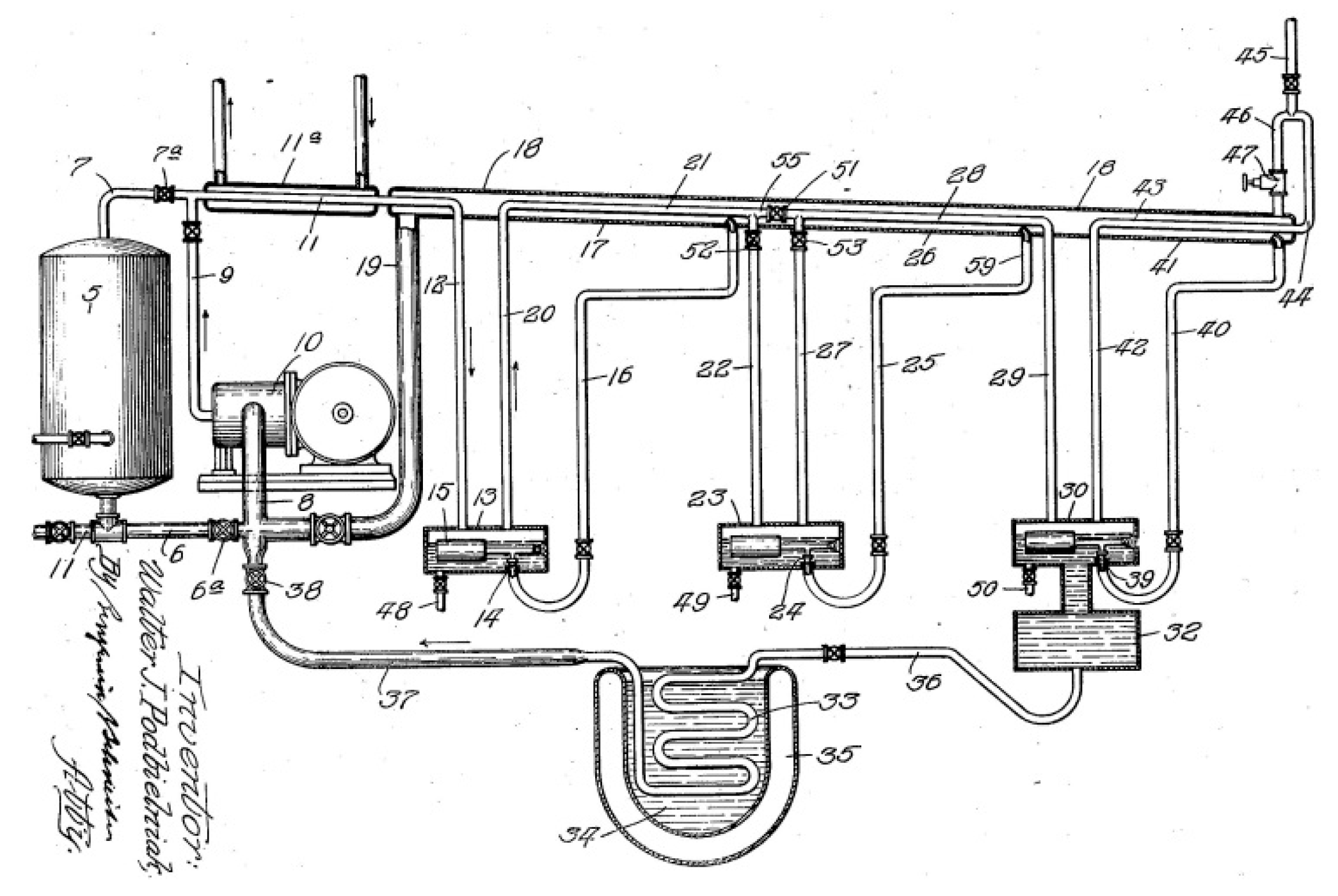
Figure 2.
Flow chart of the auto-cascade refrigerator operating with a rectifying column [6]: 1 – compressor; 2 – aftercooler; 3 – rectifying column; 4, 5 – recuperator sections; 6, 7 – expansion valves; 8 – evaporator.
Figure 2.
Flow chart of the auto-cascade refrigerator operating with a rectifying column [6]: 1 – compressor; 2 – aftercooler; 3 – rectifying column; 4, 5 – recuperator sections; 6, 7 – expansion valves; 8 – evaporator.
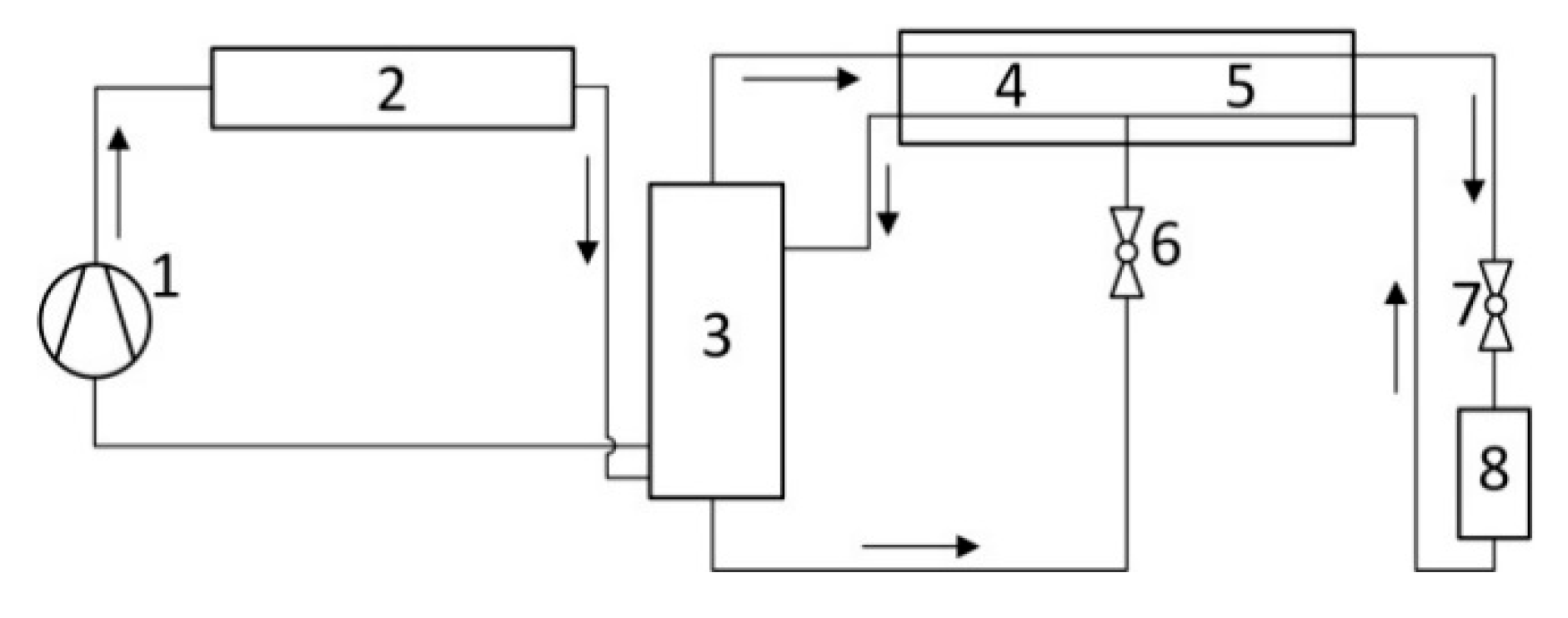
Figure 3.
Flow chart of the ACC with the only one phase separator, two evaporators and a triple-section internal RHEX. I - compressor; II – fan; III – after-cooler; IV - filter-drier; V - liquid phase separator; VI, VIII – throttle capillaries; VII – high-temperature evaporator (optional); IX - low-temperature evaporator; X, XI, XII – sections of the recuperative heat exchanger; XIII - filling valve.
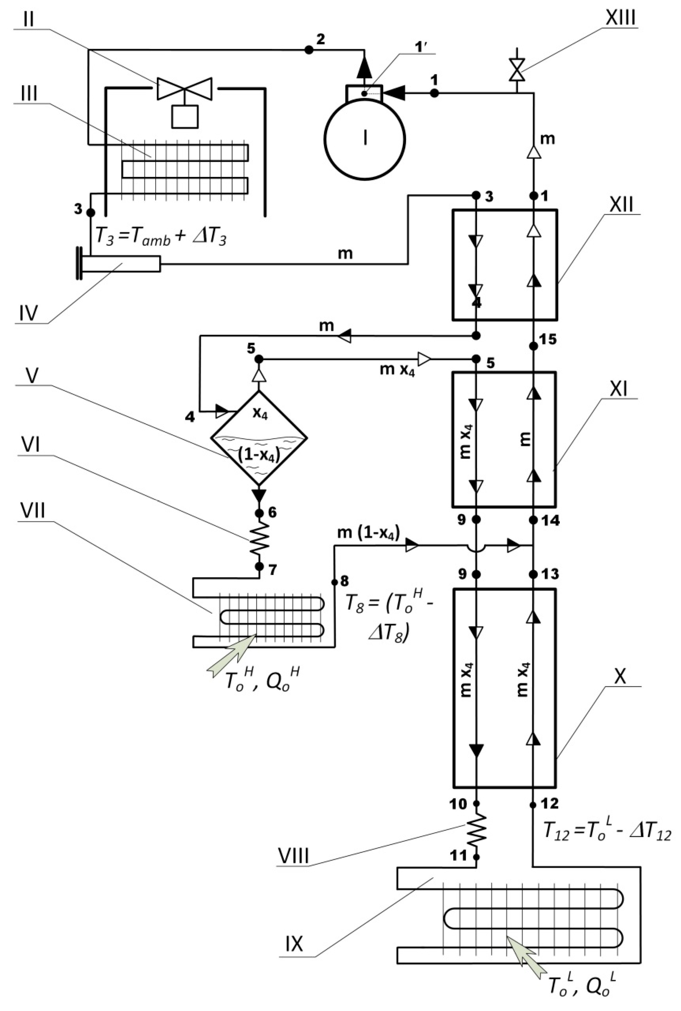
Figure 4.
Thermodynamic cycle of the LTRM operating on the ACC made up from 3 interlinked p-h diagrams differing in the working mixture component concentrations: the working mixture of butane-ethane-methane; ToL = -150°С; ToH = -15°С; Pd = 12 bar; Ps = 1 bar; T4 = -10°С; numerical indexes correspond with the ACC flow chart in Figure 3; saturation lines, thermodynamic curves and processes were computed with RefProp 9.0 (NIST standard reference database 23) [9].
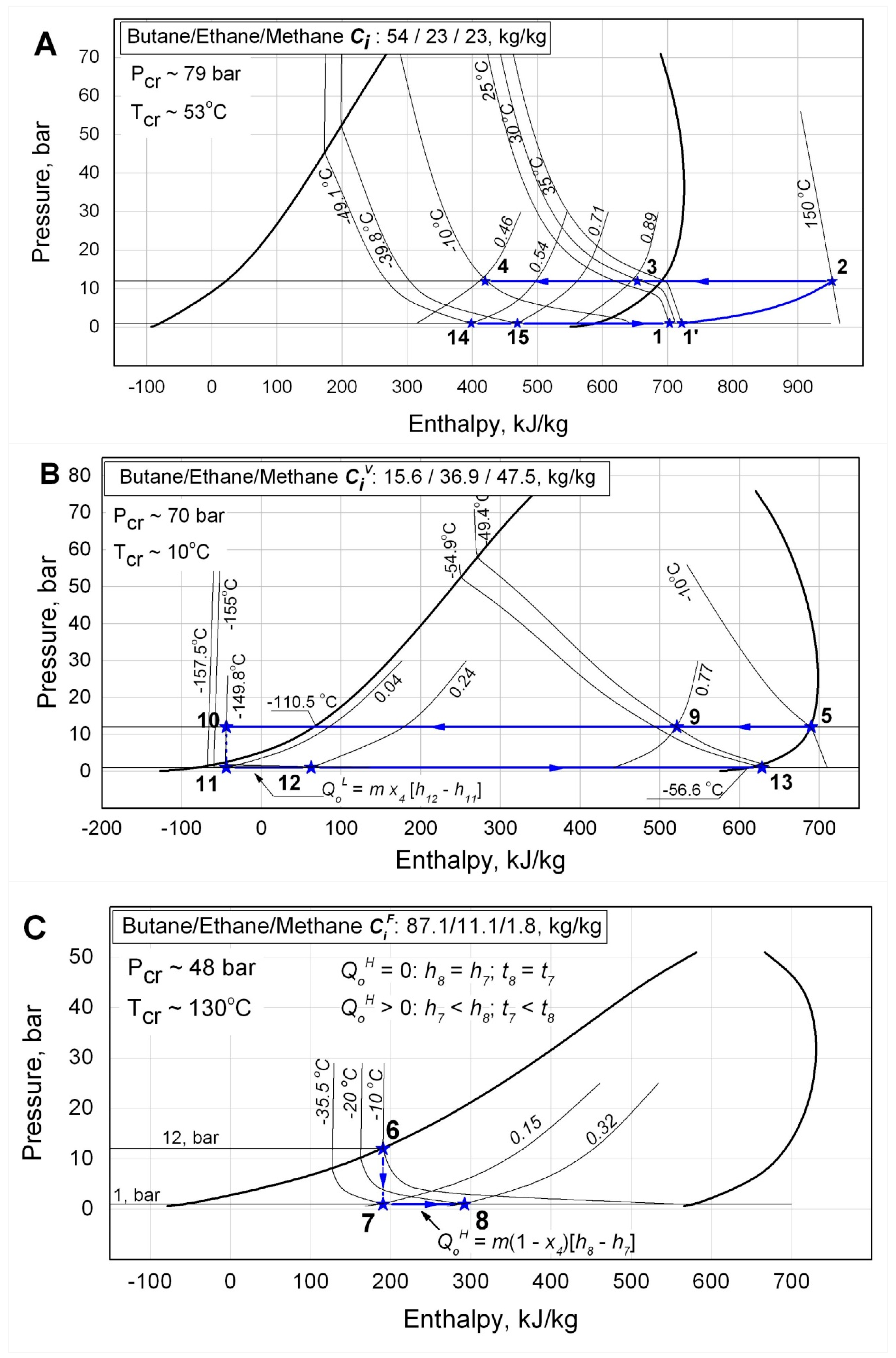
Figure 5.
The working mixture temperature changing and entropy generation at the flows 13 and 8 merging point with temperature Т13 (by the results of the ACC thermodynamic calculations: the refrigerant - zeotropic mixture of butane-ethane-methane; Ci – 0.54-0.23-0.23, kg/kg; ToL = -150°С; Pd = 12 bar; Ps = 1 bar; T4 = -10°С).
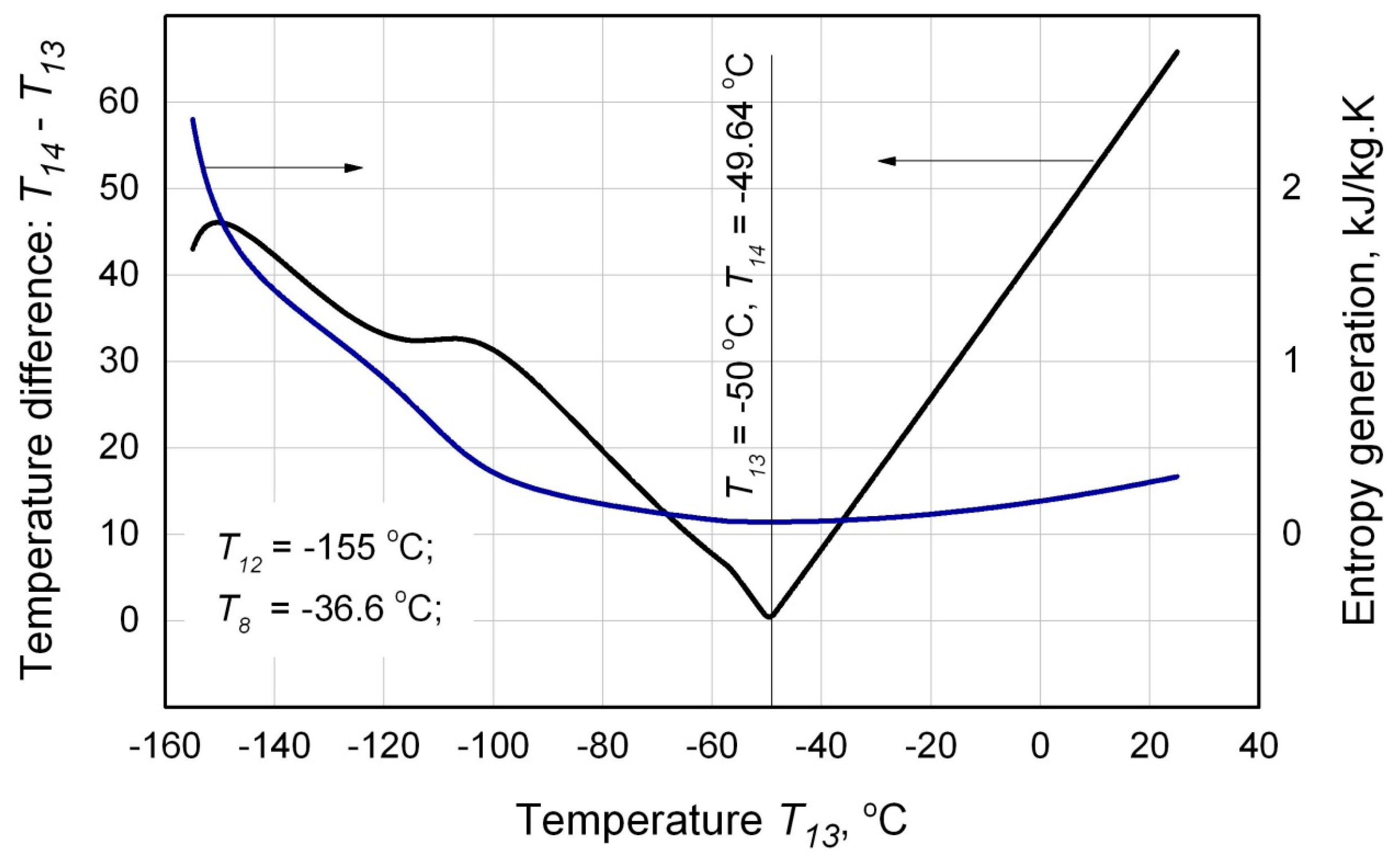
Figure 6.
Operative T-Q diagram - temperature profiles of the flows in the internal recuperative heat exchanger of the ACC refrigerator (by the results of the ACC thermodynamic calculations: the refrigerant - zeotropic mixture of butane-ethane-methane; Ci – 0.54-0.23-0.23, kg/kg; ToL = -150°С; Pd = 12 bar; Ps = 1 bar; T4 = -10°С).
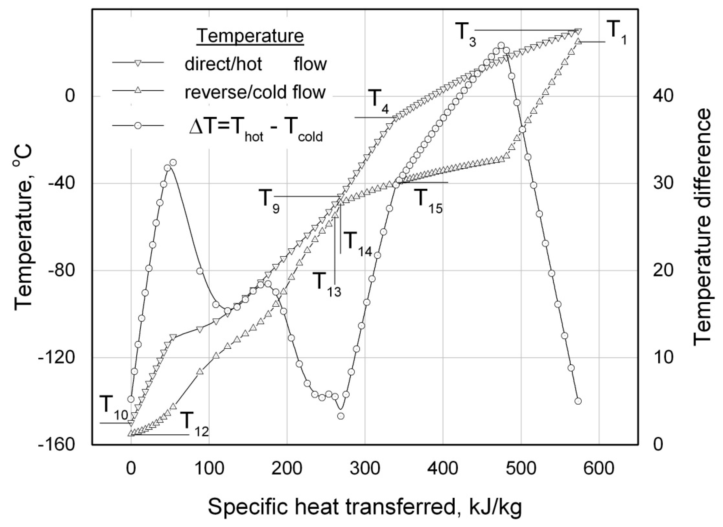
Figure 7.
Inoperative T-Q diagram - temperature profiles of the flows in the internal recuperative heat exchanger of the ACC refrigerator (by the results of the ACC thermodynamic calculations: the refrigerant - zeotropic mixture of butane-ethane-methane; Ci – 0.7-0.1-0.2, kg/kg; ToL = -150°С; Pd = 7 bar; Ps = 1.5 bar; T4 = -60°С).
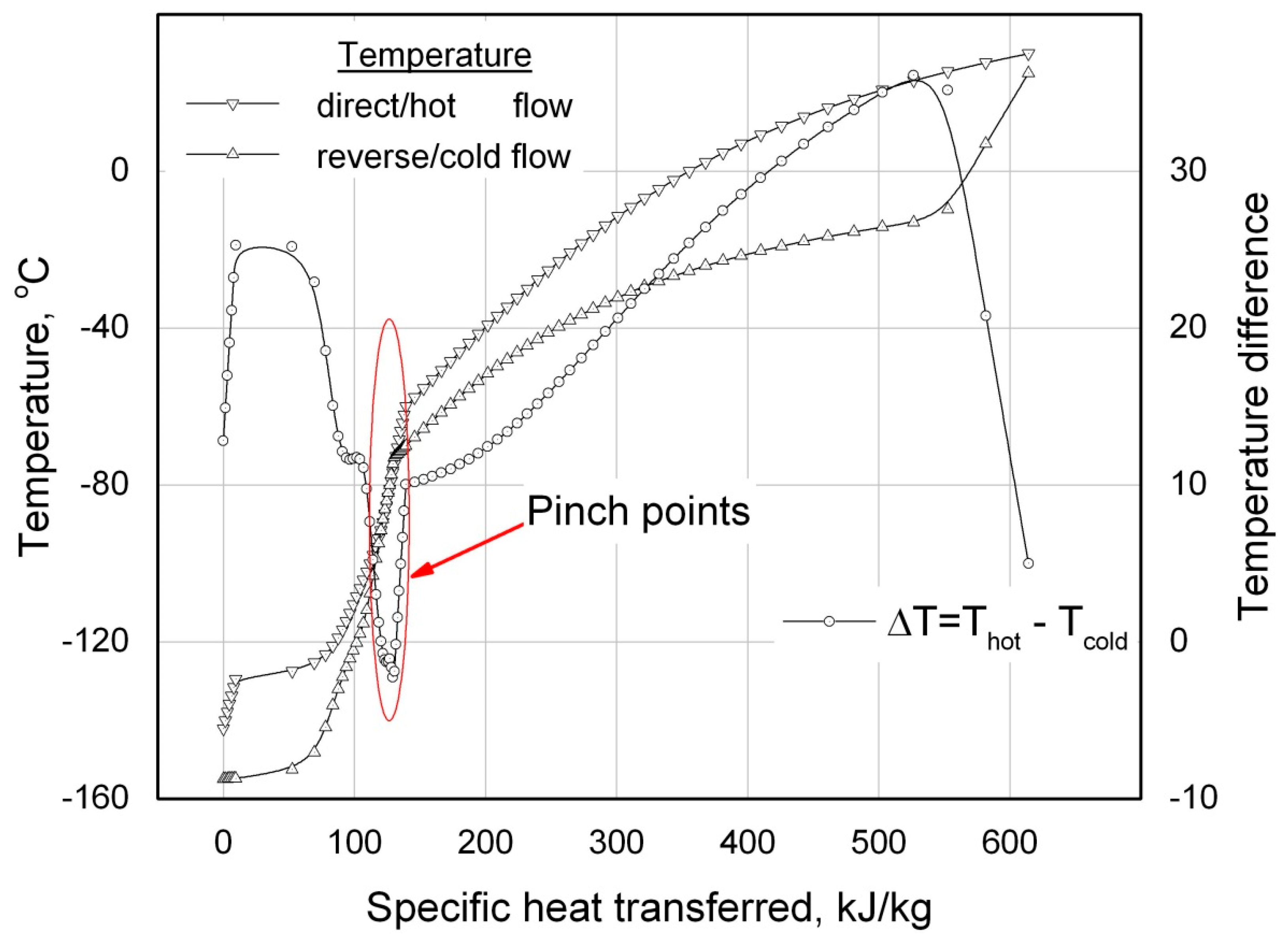
Figure 8.
The compressor input power and the temperature differences at the RHEX’s sides with the temperature of separation Т4 (by the results of the ACC thermodynamic calculations: the refrigerant - zeotropic mixture of butane-ethane-methane; Ci – 0.56-0.18-0.26, kg/kg; ToL = -150°С; Pd = 12 bar; Ps = 1 bar).
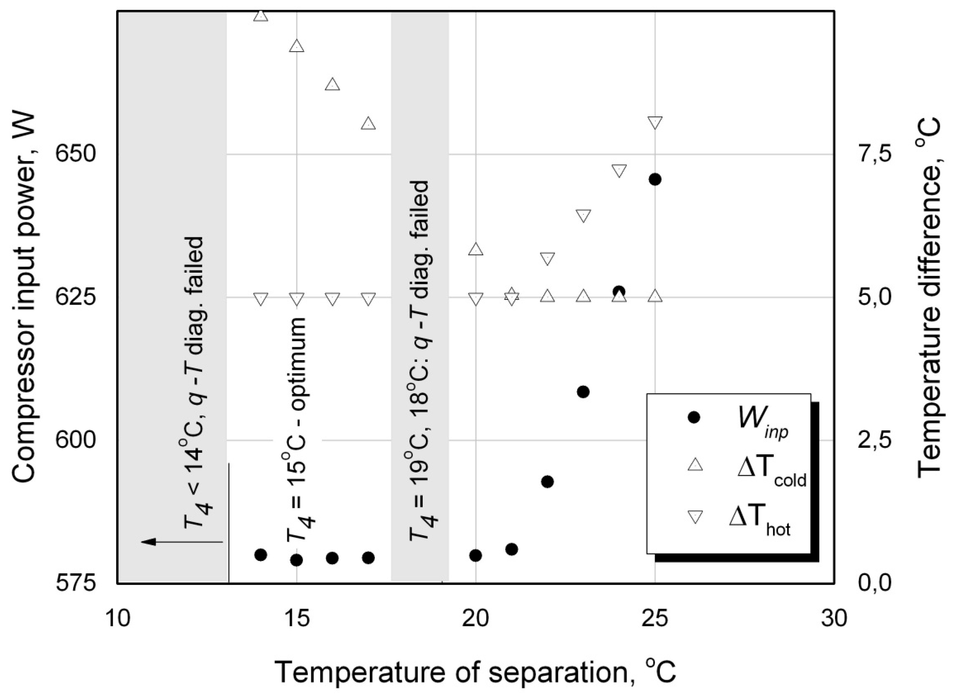
Figure 9.
The results of the ACC optimization calculations of the working mixture component concentrations: butane-ethane-methane; ToL = -150°С; Pd = 10 bar; Ps = 1 bar. А – the rapid calculations on the sparse computational grid in increments of ΔCSP = 0.10, kg/kg (the minimal/best value of Winp =1895 W under the component concentrations of: Ci: 60-10-30, kg/kg; ToL = -150°С; Pd = 10 bar; Ps = 1 bar; T4 = 19°С); B – the ACC optimization calculations on the dense computational grid in increments of ΔCSP = 0.01, kg/kg by the gradient descent procedure; C – for every set of the component concentrations calculated on the dense grid (depicted in Figure 9 B) the calculations of the optimal value of temperature of separation Т4 of the working mixture to be conducted; D – the results of the ACC optimization calculations on the dense grid should be verified for the T-Q diagrams operability (the modes with inoperable diagrams to be expelled); the minimal/best value of Winp with an operable T-Q diagram is Winp =540 W under the component concentrations of: Ci: 61-16-23, кг/кг; ToL = -150°С; Pd = 10 bar; Ps = 1 bar; T4 = 15°С;.
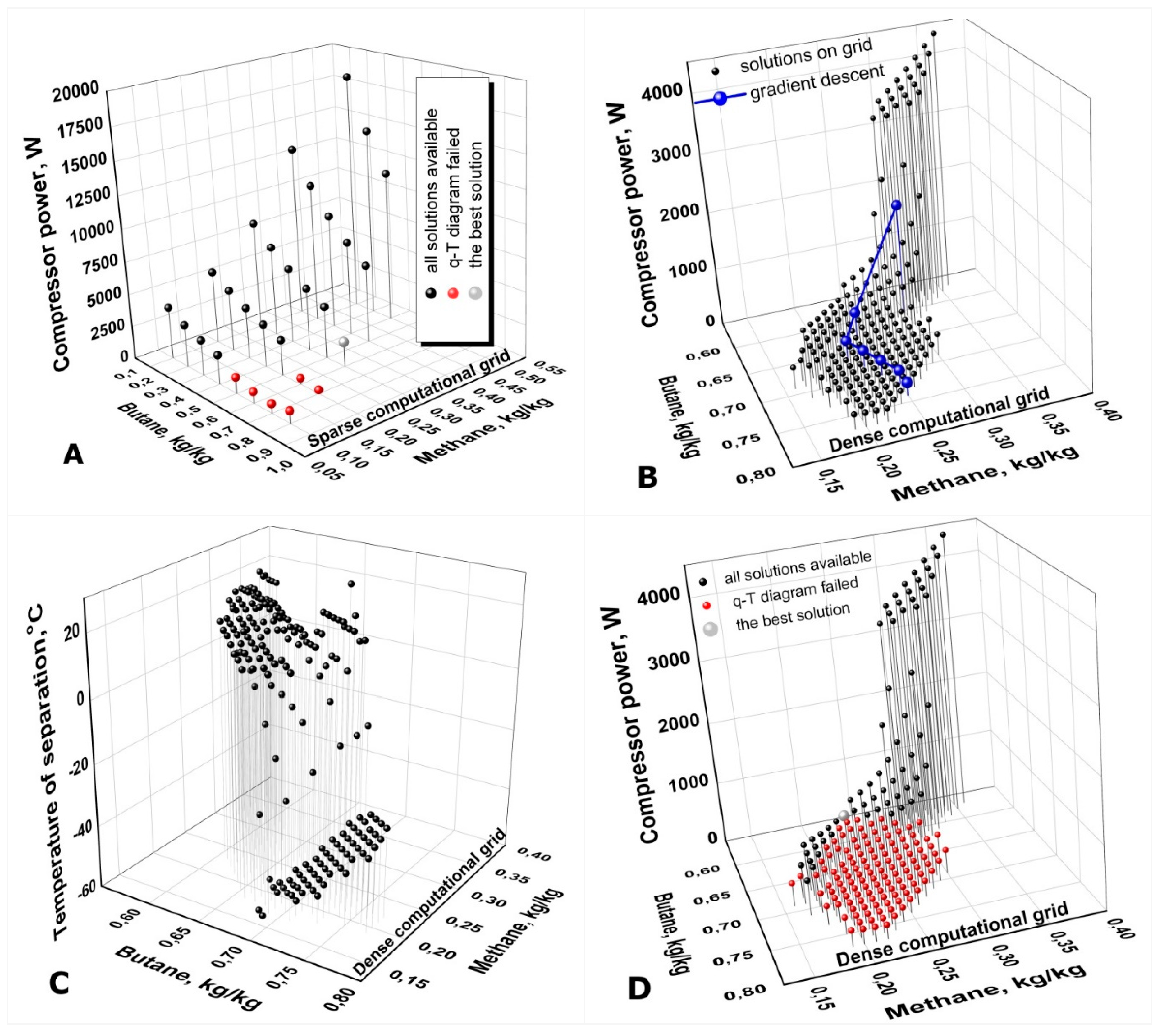
Figure 10.
The compressor’s input power with the rated mode running number from Table 1 (by the results of the ACC full-scale thermodynamic calculations: the refrigerant - zeotropic mixture of butane-ethane-methane; Ci – 0.61-0.16-0.23, kg/kg; ToL = -150°С; Pd = 10 bar; Ps = 1 bar; T4 = 15°С ).
Figure 10.
The compressor’s input power with the rated mode running number from Table 1 (by the results of the ACC full-scale thermodynamic calculations: the refrigerant - zeotropic mixture of butane-ethane-methane; Ci – 0.61-0.16-0.23, kg/kg; ToL = -150°С; Pd = 10 bar; Ps = 1 bar; T4 = 15°С ).
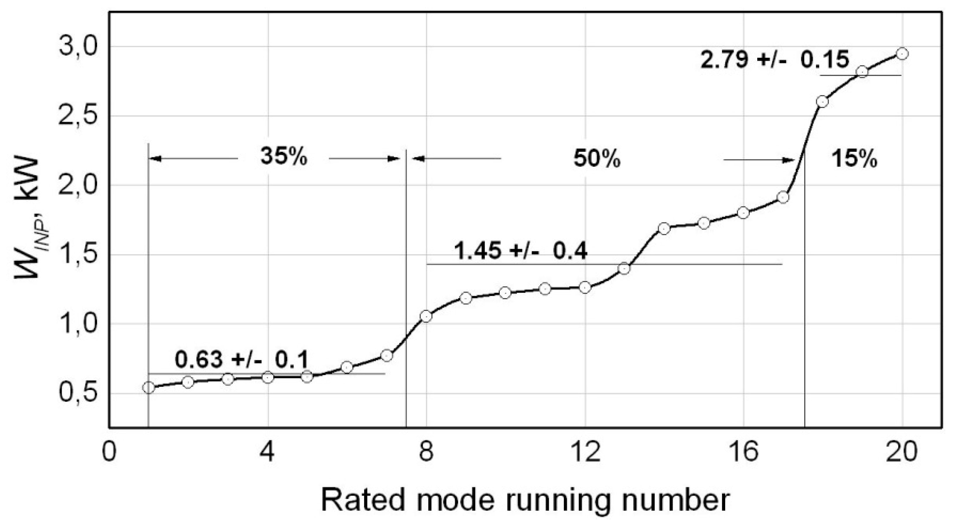
Figure 11.
The results of the ACC full-scale optimization thermodynamic calculations (butane-ethane-methane; Ci: 0.61-0.16-0.23, kg/kg;ToL = -150°С; Pd = 10 bar; Ps = 1 bar; T4 = 15°С ).
Figure 11.
The results of the ACC full-scale optimization thermodynamic calculations (butane-ethane-methane; Ci: 0.61-0.16-0.23, kg/kg;ToL = -150°С; Pd = 10 bar; Ps = 1 bar; T4 = 15°С ).
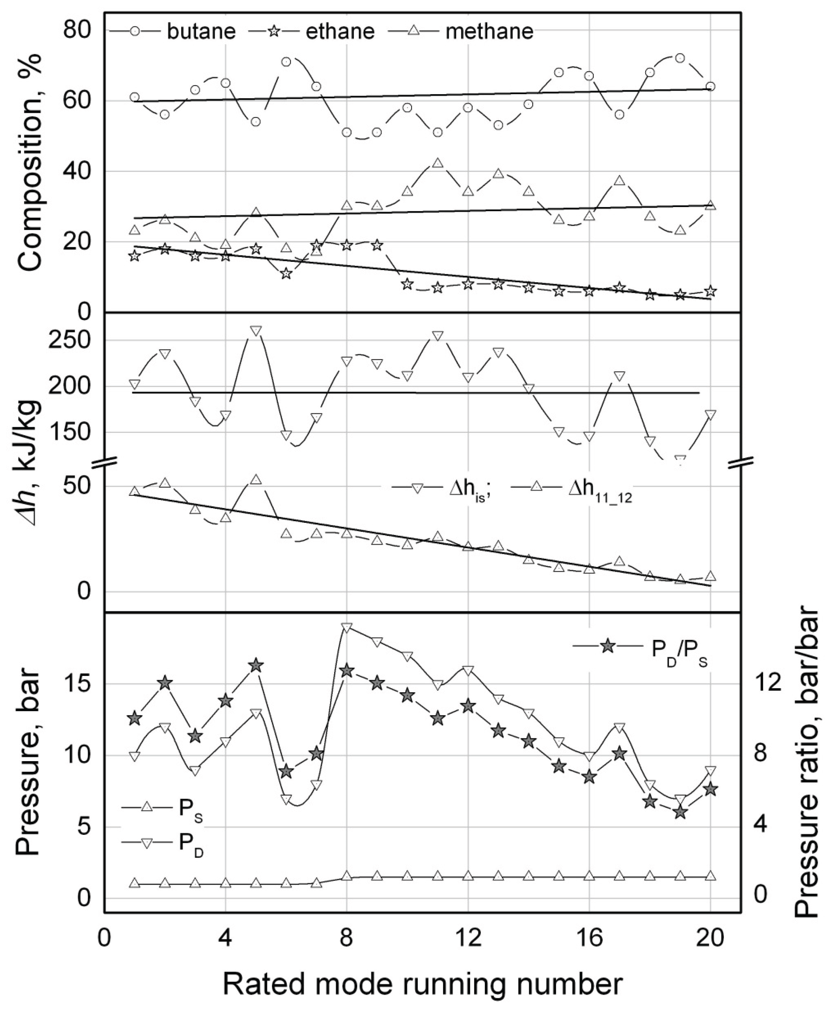

Table 1.
The results of the ACC full-scale optimization thermodynamic calculations.
| N/N | Pressure, bar | ψ, bar/bar | Concentrations, % |
Winp, kW |
Δhis |
m, g/s |
T4, oC |
ΔT3-1 | ΔT10-12 | |||
|---|---|---|---|---|---|---|---|---|---|---|---|---|
| Ps | Pd | butane | ethane | methane | kJ/kg | |||||||
| 1 | 1 | 10 | 10 | 61 | 16 | 23 | 0.54 | 203.3 | 2.1 | 15 | 5.1 | 5.0 |
| 2 | 1 | 12 | 12 | 56 | 18 | 26 | 0.58 | 236.3 | 1.9 | 15 | 5.0 | 9.4 |
| 3 | 1 | 9 | 9 | 63 | 16 | 21 | 0.60 | 184.3 | 2.6 | 11 | 5.0 | 6.5 |
| 4 | 1 | 11 | 11 | 65 | 16 | 19 | 0.61 | 169.5 | 2.9 | 15 | 47.6 | 5.0 |
| 5 | 1 | 13 | 13 | 54 | 18 | 28 | 0.62 | 261.5 | 1.9 | 15 | 5.0 | 15.1 |
| 6 | 1 | 7 | 7 | 71 | 11 | 18 | 0.68 | 148.0 | 3.7 | 11 | 5.0 | 13.1 |
| 7 | 1 | 8 | 8 | 64 | 19 | 17 | 0.77 | 167.0 | 3.7 | -4 | 5.0 | 5.0 |
| 8 | 1.5 | 19 | 12.7 | 51 | 19 | 30 | 1.06 | 228.1 | 3.7 | -60 | 42.5 | 5.0 |
| 9 | 1.5 | 18 | 12 | 51 | 19 | 30 | 1.18 | 225.3 | 4.2 | -60 | 39.8 | 5.0 |
| 10 | 1.5 | 17 | 11.3 | 58 | 8 | 34 | 1.22 | 212.4 | 4.6 | -24 | 48.2 | 5.0 |
| 11 | 1.5 | 15 | 10 | 51 | 7 | 42 | 1.25 | 256.0 | 3.9 | -15 | 5.0 | 5.0 |
| 12 | 1.5 | 16 | 10. 7 | 58 | 8 | 34 | 1.26 | 210.7 | 4.8 | -25 | 43.6 | 5.0 |
| 13 | 1.5 | 14 | 9.3 | 53 | 8 | 39 | 1.40 | 237.8 | 4.7 | -24 | 9.3 | 5.0 |
| 14 | 1.5 | 13 | 8. 7 | 59 | 7 | 34 | 1.69 | 198.5 | 6.8 | -21 | 28.9 | 5.0 |
| 15 | 1.5 | 11 | 7.3 | 68 | 6 | 26 | 1.73 | 151.7 | 9.1 | -24 | 45.4 | 5.0 |
| 16 | 1.5 | 10 | 6. 7 | 67 | 6 | 27 | 1.80 | 146.9 | 9.8 | -25 | 37.0 | 5.0 |
| 17 | 1.5 | 12 | 8 | 56 | 7 | 37 | 1.91 | 212.3 | 7.2 | -20 | 6.0 | 5.0 |
| 18 | 1.5 | 8 | 5.3 | 68 | 5 | 27 | 2.60 | 141.4 | 14.7 | -23 | 5.0 | 7.9 |
| 19 | 1.5 | 7 | 4. 7 | 72 | 5 | 23 | 2.81 | 121.0 | 18.6 | -29 | 5.0 | 7.3 |
| 20 | 1.5 | 9 | 6 | 64 | 6 | 30 | 2.95 | 161.4 | 14.6 | -24 | 5.0 | 6.4 |
Disclaimer/Publisher’s Note: The statements, opinions and data contained in all publications are solely those of the individual author(s) and contributor(s) and not of MDPI and/or the editor(s). MDPI and/or the editor(s) disclaim responsibility for any injury to people or property resulting from any ideas, methods, instructions or products referred to in the content. |
© 2025 by the author. Licensee MDPI, Basel, Switzerland. This article is an open access article distributed under the terms and conditions of the Creative Commons Attribution (CC BY) license (https://creativecommons.org/licenses/by/4.0/).
Copyright: This open access article is published under a Creative Commons CC BY 4.0 license, which permit the free download, distribution, and reuse, provided that the author and preprint are cited in any reuse.


