Submitted:
05 September 2025
Posted:
05 September 2025
You are already at the latest version
Abstract
The primary goal of this paper was to look into the existence of a debt Laffer curve in the Bangladesh economy. Then, using this goal, find a debt level that maximises economic growth. This study used the debt-to-GDP ratio variable as the X-axis variable in the debt Laffer curve analysis. Real GDP is used as an economic growth indicator variable. Another goal of this study was to use the quantile regression technique to examine the relationship between external debt and economic growth. Quantile regression helped us investigate associations outside the dependent variable's mean, which often remain unseen. Aside from the external debt, various other economic growth indicators were evaluated. We used yearly time series data from 1977 to 2020 from the World Bank's World Development Indicators. Based on our findings, the debt Laffer Curve does not exist, so a debt threshold level cannot be established for the Bangladesh economy. The examination of quantile regression estimates allowed us to investigate previously unknown relationships, such as the negative marginal effect of the debt overhang variable on real GDP increases, as the real GDP increases. This pattern was not seen when we applied OLS.
Keywords:
Debt Laffer curve
; Debt-to-GDP ratio
; External Debt
; OLS
; Quantile Regression
; Real GDP
1. Introduction
Bangladesh gained independence in 1971. It has made significant progress in various sectors since gaining independence. Bangladesh, once one of the world’s poorest countries, has experienced remarkable economic growth over the last two decades. It was once referred to as a ‘bottomless basket’ (Dhaka Tribune, 2018), but it is now one of the world’s five fastest-growing economies. Its status will now be changed from Least Developed Country (LDC) to developing country. The government’s goal of becoming a developed country by 2041 has become a reality. According to the IMF, Bangladesh’s economy will grow from 180 billion US dollars to 322 billion US dollars by 2021 (World Bank, 2019). The government of Bangladesh has been considering a variety of mega-projects to propel its economy into the next gear. This is good news, but Sri Lanka’s recent financial mess should give us something to think about. These mega-projects are funded mainly by Russia, Japan and China. Bangladesh has to repay the most debt to Russia, Japan and China, with 36.6% of the total debt repayment owed to Russia, 35% to Japan and 21% to China (Bhattacharya, 2022).
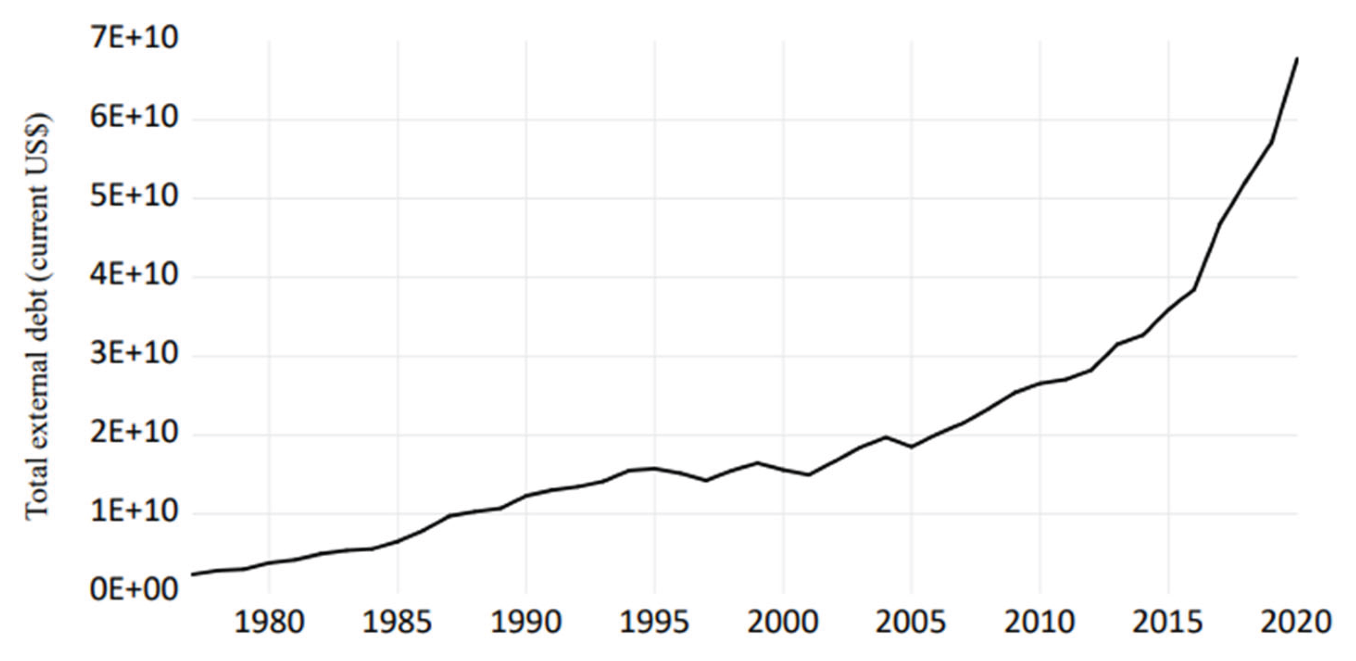
A country’s foreign debt may be a tremendous weapon for investment and growth, provided it is managed well. External debt is the portion of a country’s overall debt owed to lenders outside of the country’s boundaries. People, businesses, and governments can be liable for debts (Farhana and Chowdhury, 2014). Often, due to a lack of financial and economic resources, emerging countries are forced to borrow. As a result, governments in developing nations rely on external borrowing as a source of revenue (Okungbowa et al., 2018). If the debt service costs are low compared to the returns of the investment, it can boost investment levels and boost the economy’s growth rate, but if the costs are excessive, it can limit growth (Farhana and Chowdhury, 2014). The fiscal policy relies heavily on taxation as a source of revenue, but it is not always adequate to satisfy the demands. To finance its deficit balance of payments and save investments gap, Bangladesh relied on external loans (Yeasmin et al., 2015). Bangladesh’s external debt grew by 125 per cent over the decade, from 25.3 billion US dollars in 2009 to 57 billion US dollars in 2019, according to the data of World Bank. A high amount of debt can impair government operations since debt is a long-term expense that cannot be reduced during fiscal difficulty. If external debt has a detrimental impact on economic growth, either directly or indirectly, policymakers must be mindful of these links while developing and implementing macroeconomic policy.
Figure 1.
Data visualization of total external debt of Bangladesh over the years.
According to Okonjo-Iweala et al. (2003), countries borrow for two fundamental reasons: macroeconomic reasons to support additional investment or higher consumption, to finance the transitory balance of payments deficits while benefiting from cheaper nominal interest rates overseas, and to evade severe budget limitations. This implies that countries can borrow to encourage economic growth and decrease poverty. He maintained that when debt exceeds a certain threshold, it begins to have a negative influence since debt servicing becomes an enormous burden and governments find themselves on the wrong side of the debt Laffer curve, with debt restricting investment and growth. It is widely accepted that excessive levels of foreign debt are detrimental to an economy. Thus the analysis to investigate the existence of a Debt Laffer curve could be helpful for a country to understand when debt reduction is necessary. It also defines contractual conditions and responsibilities for loans regarding the net value.
For developing countries, there are several types of research on the GDP and debt to dig out the relationship between these time series variables, identify the long-run or short-run relationship and predict using the best-fitted model. Chaudhary et al. (2001) described the debt Laffer curve approach for South Asian nations to determine if debt reduction was advantageous for these nations. In this work, OLS estimations and price elasticity were applied through time series analysis. From 1970-71 to 1994-95, data for analysis were collected for all South Asian countries. Pakistan, Bangladesh, Nepal, Sri Lanka, and India were found to be on the right side of the debt Laffer curve. Islam and Biswas (2005) undertook a study to examine Bangladesh’s debt composition, debt financing, and its implications, as well as its debt sustainability. For the sample period of FY 1981 to FY 2005, debt dynamics have been evaluated using equations of sustainability. During the study sample period, their research revealed that the interest rate component had a more significant impact on the total debt stock than the growth component. The variables of debt dynamics revealed that Bangladesh’s debt-to-GDP ratio is sustainable. Chowdhury and Mavrotas (2006) investigated the cause-and-effect link between foreign debt and economic slowdown. Granger causality tests were undertaken using data from indebted developing nations of Asia and the Pacific. These tests suggested that the external indebtedness of developing nations is a symptom rather than a cause of the economic slowdown is false. Estimation results reveal that the full effects of public and private foreign debts on GNP are negligible and opposite. However, an increase in GNP significantly increases public and private external debts. Hyman (2007) examined the effect of a high debt burden on the economic growth of six Caribbean nations. He discovered that the high levels of debt in these small Caribbean nations result in a negative economic growth rate. Ramesh Chand Paudel and Nelson Perera (2009) examined the cointegrated relationship between real GDP growth, trade openness, labour force, and foreign debt in Sri Lanka from 1955 to 2006. The study finds that all variables positively affect real GDP growth, with the labour force being the most influential variable. Tahir et al. (2015) have examined the external factors of GDP growth using the data from the Pakistan Bureau of Statistics. The study ensures that remittance has a long-run relationship with GDP growth, which is significant. The remittance affects the investment and other factors which control the improvement of the GDP growth. This result can be generalised to other developing countries. Mohsin et al. (2021) studied the impact of South Asia’s external debt on GDP growth. World Bank data were analysed using panel ordinary least square (OLS) and Quantile regression from 2000-2018. The research showed that while high levels of external debt are detrimental to economic expansion, holding a large amount of debt in the form of a stock helps growth. From this discussion, it can be said that there is a lack of literature that conducts any econometric study considering the debt Laffer curve and quantile regression for Bangladesh jointly.
This study’s primary objective is to determine whether or not the Bangladeshi economy has a debt Laffer curve. And, based on the outcomes of this objective, to determine the optimal debt level for maximum economic growth. Then, we will examine the relationship between economic growth and external debt using quantile regression. Quantile regression reveals how factors interact outside of the data’s mean. Keeping this information in mind, the study objectives are as follows:
- To examine how Bangladesh’s economic growth is affected by the country’s mounting external debt.
- To investigate if the Bangladesh economy has a Debt Laffer Curve.
- To determine the extent to which Bangladesh’s external debt burdens the economy.
- To observe the change in the marginal effects of debt on real GDP for different levels of real GDP using quantile regression.
2. Material and Methods
This study aimed to explain Bangladesh’s debt dynamics using a Quantile regression model and to determine whether the Bangladesh economy has a debt Laffer curve. This study utilised annual time series data spanning 44 years, from 1977 to 2020. All of this study’s data comes from the World Bank Database. This analysis employs the following explanatory variables: External debt to GDP ratio, External debt stocks, Total reserves to External debt ratio, Official exchange rate, Trade openness, and Exports. The only dependent variable accepted as an economic indicator variable is Real GDP.
2.1. Time Series Testing Methodology
In the light of econometrics from many preliminary steps of using time series data in the analysis, the test of stationary or non-stationary is the most usable and valid. From the different levels of being stationary, the macroeconomic analysis varies. The Augmented Dickey-Fuller (ADF) test has been used in this paper to check for stationarity in the time series variables. The hypothesis to be tested is:
For this test, if the null is accepted, the unit root is present in the data, which refers to the data being non-stationary. The alternative represents the stationarity of the data (Dickey & Fuller, 1979).
2.2. Multiple Linear Regression
When a dependent response variable should be approximated from several independent variables, multiple linear regression is used. The model is set in the following way:
Where represents the response variable, and the represents the regressor variables. The normally distributed error term is denoted by The term is the intercept, and , , ..., represent the regressor coefficients for each of the regressor variables, and these regressor coefficients will be estimated. There is number of observations and number of regressor variables (Montgomery et al., 2021). To estimate the regression coefficients, Ordinary Least Squares (OLS) and Quantile Regression techniques are used in this study.
2.3. Ordinary Least Squares
The method of ordinary least squares, OLS, can be used to estimate the regression coefficients . It is assumed that the error term in the model has , and that the errors are uncorrelated. These estimates are found by minimising the distance from the observations to the fitted values also called residuals. The least-squares function can be expressed as:
And should be minimised with respect to , , ..., . When using matrix notations, the least squares function is given by Montgomery et al. (2021).
2.4. Quantile Regression
In 1757, Roger Joseph Boscovich proposed a method to fit a regression line to some data by minimising the Least Absolute Deviation (LAD) (Koenker and Bassett, 1978). The Quantile Regression (QR) (Koenker and Bassett, 1978) is an extension of this concept. It comes from the realisation that if the absolute value function is tilted around the origin, instead of obtaining the conditional median, we obtain a conditional model of the cumulative density function of the response. Thus, quantile regression minimises a weighted sum of the positive and negative error terms:
Where is the quantile level. For each quantile level , the solution to the minimisation problem yields a distinct set of regression coefficients. It can be noted that corresponds to the median regression.
The average impact of independent variables on the ‘average dependent variable’ may be evaluated using the ordinary least squares regression approach with point estimates While the ‘average’ is a good place to start for analysis, it can obscure other significant aspects of the connection. “The regression curve summarises the averages of the distributions corresponding to the set of x’s,” says Mosteller and Tukey (1977). We can additionally construct many regression curves that correspond to the different percentage points in the distributions to offer a full picture of the set. Most of the time, this does not occur, and as a result, least square regression estimates rarely provide us with the complete picture. Similarly to how the mean only provides a partial image of a single distribution, the regression curve only provides a partial view of numerous distributions. As a result, quantile regression tools can help us better understand the link between real GDP and its drivers in this study. Also, the requirement that the error components are normally distributed across the conditional distribution is relaxed by employing a quantile regression method. By removing this restriction, we could investigate whether or not the conditional distribution of all determinants of real GDP exhibits variation in the slope parameters predicted for different quantiles.
2.5. Diagnosis of OLS and QR
The Breusch-Godfrey-Bertolo LM test is used in this paper to detect autocorrelation in our fitted OLS model. The Breusch-Godfrey serial correlation uses the lagrange multiplier testing procedure (Gujarati, D.N., 2003). For this test, the test hypothesis can be written as,
The variance inflation factor (VIF) has been used here to assess the degree of multicollinearity among independent variables. The larger the value of VIF presents of more severe multicollinearity. If the value of VIF exceeds 10, it is considered that the variable is highly collinear (Gujarati,D.N., 2003).
The Glejser test and the Brueush-Pagan test has been used here for detecting heteroscedasticity. For heteroscedasticity the hypothesis to be tested is,
By testing this hypothesis the decision can be made that if the model is preferable or not.
The Jarque Bera normality test is used to see if the residual follows the normality assumptions. The normality test can be done for following hypothesis:
Thus the test defines whether the use of the OLS is preferable or not.
Testing for stability is also necessary for determining model viability (Ramsey, 1969). In this research, we examine the stability of the data using the Ramsey Reset procedure. The Ramsey reset test’s null hypothesis states that the model is stable, while the alternative states that it is not.
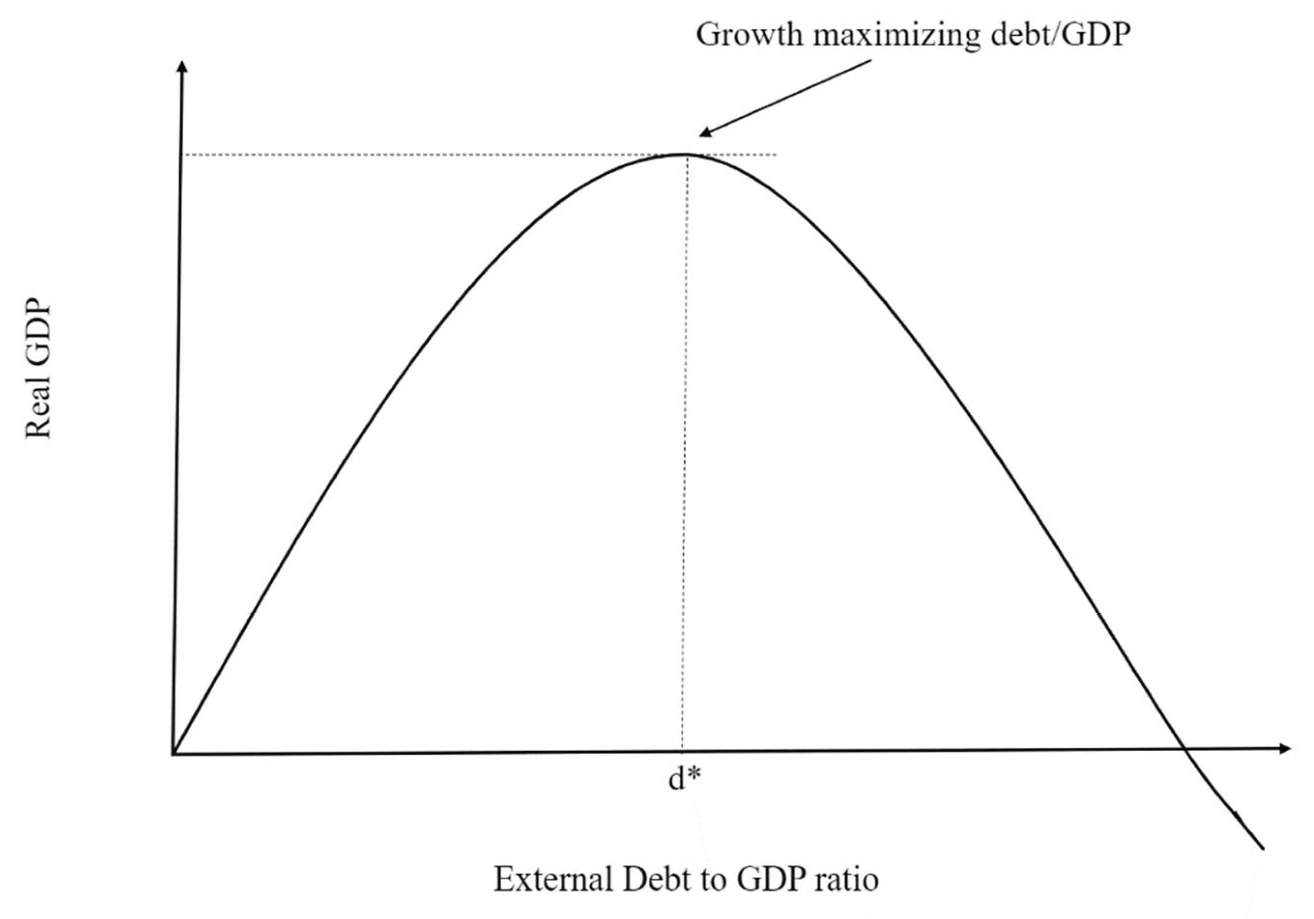
2.6. Debt Laffer Curve
The Laffer curve was utilised to maximise tax collection in an effort to eliminate or minimise the fiscal deficit. The overall architecture of the Laffer debt curve is proposed by Krugman (1988) and Sachs (1990) in support of the concept that an accumulation of public debts over a particular level is overloaded by GDP. This setting can be tested with a quadratic setting. This specification is a better alternative to the Reinhart and Rogoff (2010) method as threshold levels are set by a process of optimisation (instead of being chosen in a discretionary way).
The Laffer curve consists of two parts: an “advantageous” segment in which low public debt boost GDP and a “disadvantageous” section in which high levels of public debt damage GDP. Therefore, the two portions are split by a perfect threshold. This ‘optimality’ is only seen from the point of view of leverage and should not be taken as optimisation of economic welfare (Bhimjee and Leão, 2020).
There are numerous reasons why the debt Laffer curve study is beneficial. First, it demonstrates when debt reduction might be advantageous for a nation (when a country is on the wrong side of the curve). Second, the debt Laffer curve can be applied to debt reduction strategies. In addition, the debt Laffer curve can be used to set contractual conditions and loan obligations in terms of net present value.
Figure 2.
A debt Laffer Curve.
Different model specifications are applied for analyzing non-linearity in the debt and growth relationship. For the objective of finding a debt Laffer curve, the quadratic specification of the debt stock variable, popular in the empirical literature, is employed by Hansen(1999). The quadratic specification is in the following form:
Where is real GDP, is a constant or an individual specific effect (intercepts), is external debt as a ratio of real GDP, is squared of external debt-to-GDP ratio, and is the vector of other control variables, is the unobserved error term, and is the representation of time. To find the turning point simple maximisation problem is solved by taking the first derivative of the significant coefficient of and holding all other variables constant.
and solving for zero gives:
If the value for coefficient is negative, we solve for the maximum point and do the opposite if the value is positive. Therefore, if regression gives a coefficient for other than negative the hypothesis of inverted U-relationship is rejected, but not the non-linear relationship of debt and growth (Hansen, B.E., 1999).
2.7. Cointegration Test
Cointegration test is necessary to establish a long run relationship among our discussed variables. This study has utilised the Engle-Granger two step procedure to check for cointegration among the variables. The two-step Engle-Granger technique begins with the creation of residuals based on the classical regression, which are then examined for the presence of unit roots (Engle & Granger, 1987). The ADF test can be used to determine the stationarity of residuals. The hypothesis for the ADF test can be written as,
If the P-value of the test statistic is larger than the specified significance level, the null hypothesis may be rejected. Rejecting the null hypothesis results in the stationarity of the residual series, indicating that the variables are cointegrated.
3. Results and Discussion
3.1. Univariate Analysis

Table 1.
Univariate analysis of the variables.
| Variable | Mean | Standard deviation |
|---|---|---|
| Real GDP | 1.02e+11 | 6.73e+10 |
| External debt to GDP ratio | 18.25787 | 4.408501 |
| External debt stocks | 1.96e+10 | 1.49e+10 |
| Debt service on external debt | 6.72e+08 | 4.83e+08 |
| Total reserves to debt ratio | 24.50982 | 22.9162 |
| Official exchange rate | 50.25002 | 22.6975 |
| Trade openness | 29.00904 | 9.612027 |
| Exports | 1.19e+10 | 1.37e+10 |
3.2. Analysis Using the Debt Laffer Curve
For a long time, academics and policymakers have debated the relationship between debt and economic growth (Osinubi & Olaleru, 2006). Even now, no one can agree on a single viewpoint on how debt affects growth. Mankiw et al. (1992) proposed a classic theory that includes both effects and concludes that, in the short run, public debt has a positive influence on growth by putting greater focus on aggregate demand, but in the long run, it has a negative effect due to the crowding-out effect. The crowding out effect is an economic theory that states that when government spending increases, private spending decreases or even ceases. Most empirical time series studies reported in the literature that looked at the relationship between external debt and growth in the short and long run showed either negative or insignificant findings. Using solely the stock variable of external debt as an explanatory variable is assumed to be the reason for the non-significant results.
This study took a different approach by using the debt-to-GDP ratio as the debt variable and attempted to discover the effect of debt overhang (Krugman, 1988) and debt service in the long run, as well as test one of the research objectives, namely the existence of an inverted U-shaped relationship between external debt and growth for the Bangladesh economy. The threshold level when the sign of impact changes has been explored is based on the existence of the debt Laffer curve. We specified the following quadratic function for estimation:
Where is the Real GDP (data are in constant 2015 prices). is the External Debt to GDP ratio, which can also be called the debt overhang Variable (the standard debt indicator used in this study to estimate the debt overhang effect is the debt/GDP ratio) (Krugman, 1988). is the square of the External Debt to GDP ratio. is the amount of service payment of external debt. is the Official exchange rate. is the total reserve to external debt ratio. denotes trade openness, which is the total of goods and services exports and imports expressed as a percentage of GDP.
3.2.1. Autocorrelation Test
Table 2.
Autocorrelation test result.
| Method | p-value | decision |
|---|---|---|
| Breusch-Godfrey lagrange multiplier | 0.6427 | Accepted |
From the above table it has been shown that the p-value for Breusch-Godfrey lagrange multiplier test is 0.6427 which is greater than 5 percent level of significance. So we may not rejected null at 5 percent level of significance and conclude that there exists no serial corellation in data.
3.2.2. Heteroscedasticity Test
Table 3.
Heteroscedasticity test result.
| Method | p-value | Decision |
|---|---|---|
| Brueush-Pagan | 0.0000 | Rejected |
| Glejser | 0.0001 | Rejected |
From the above two test results, it can be said that both the results are less than a 5 percent level of significance. So null hypothesis may be rejected that is, no heteroscedasticity exists in the data set. Despite heteroscedasticity, OLS estimators are linearly unbiased. So, we proceeded with our analysis of the existence of a Debt Laffer curve, even though the data contain heteroscedasticity (Gujarati, D.N.,2003).
3.2.3. Multicollinearity Test
Table 4.
Multicollinearity test result.
| Method | VIF | Tolerance |
| Variance Inflation Factor | 33.23 | 0.03 |
The tolerance level for the VIF test is 10. If the mean VIF were less than 10, we would conclude that there is no multicollinearity in the data (Gujarati, D.N.,2003). The obtained result is 33.23. Thus, it can be said that multicollinearity in the data is present. So, we may reject the null at a 5 percent level of significance, that is, there exists no multicollinearity. However, multicollinearity does not present a substantial challenge when is large and the regression coefficients are individually significant, as seen by higher values. This is the case when there is a positive correlation between the variables (Gujarati, D.N.,2003).
3.2.4. Jarque Bera Test for Normality
Table 5.
Jarque Bera test result.
| Method | p-value | decision |
|---|---|---|
| Jarque-bera | 0.1318 | accepted |
Considering the level of significance at 5 percent it has been found that the null hypothesis may not be rejected. So, it can be considered that the residuals are normally distributed.
3.2.5. Results of OLS
Result for the model (6) is given below:
Table 5.
OLS regression result for model (6).
| Variable | Coefficient | t-statistic | p-value |
|---|---|---|---|
| C | 6.15E+10*** | 3.183062 | 0.003 |
| DEBT | -6.30E+09** | -2.51698 | 0.0163 |
| DEBTSQ | 1.36E+08* | 1.928697 | 0.0615 |
| DEBTSERVICE | 19.27701*** | 9.218538 | 0.000 |
| EXCHANGE | 2.04E+09*** | 8.712174 | 0.000 |
| RESERVE | 9.04E+08*** | 8.692363 | 0.000 |
| TRADE | -1.27E+09*** | -3.49074 | 0.0013 |
Here, cell entries are coefficients, with p-value in parentheses and *** represent the significance at the 1% levels, ** represent the significance at the 5% levels, * represent the significance at the 10% levels.
Strong evidence exists that a smooth inverted U-shaped debt Laffer curve does not exist, as the coefficients of the debt overhang variable (detb-to-GDP ratio) and its squared value did not satisfy the requirements for an inverted-U type quadratic relationship, namely a positive and significant coefficient for the debt overhang variable and a negative and significant coefficient for the square of the debt overhang variable (Hansen, B.E., 1999).
With an R-squared value of 98% and an F-statistic of 530.8335, the overall fit is good. This F-statistic is extremely significant, passing the significance test with a confidence level of 1 percent. Thus, the hypothesis of a smooth inverted U-shaped debt Laffer curve for Bangladesh may be rejected. That means a debt Laffer curve does not exist in Bangladesh economy.
It can be noted that the trade variable has a negative coefficient and it is highly significant, effortlessly passing the significance test at the 1 percent confidence level. This might be attributed to the country’s inadequate conflict management mechanisms and lack of high-quality institutions and the imbalance between exports and imports (Ali and Abdullah, 2015). It could also happen because our sample behaves like this way.
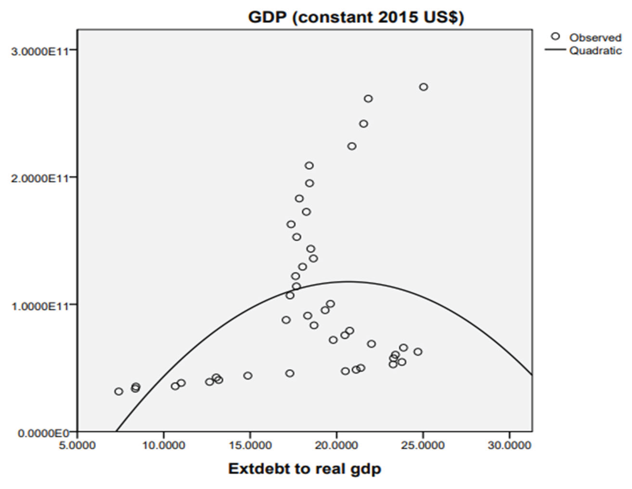
We can confirm our conclusion by fitting a quadratic curve to the scatter of the GDP against debt overhang variable. This is accomplished using the SPSS software package. The graph is displayed in Figure 3. From the graph, it is evident that the observed data points do not fit properly with an inverted U shaped quadratic curve. Thus our study finding is graphically verified.
Figure 3.
Quadratic curve fitting between real GDP and External debt-to-GDP ratio.
3.2.6. Co-Integration Test
From the ADF test results, we have found the following results, shown in Table 6.
Table 6.
ADF test results.
| Variable | Stationary at |
|---|---|
| Real GDP | 2nd difference |
| External debt-to-GDP ratio | 1st difference |
| Debt-to-GDP ratio square | 1st difference |
| Debt servicing | 2nd difference |
| Official exchange rate | 1st difference |
| Total reserves to debt ratio | 1st difference |
| Trade openness | 1st difference |
| Exports | 1st difference |
The tests show that the variables real Real GDP and Debt servicing are stationary at 2nd difference. Rest of the variables are stationary at 1st difference. The following step was to see if the non-stationary variables were cointegrated. Variable differentiation to attain stationarity results in the loss of long-run qualities. Cointegration indicates that if two or more nonstationary variables have a long-run relationship, deviations from this long-run path are stationary (Engle & Granger, 1987). The Engel-Granger two-step approach was employed to establish this. This was accomplished by creating residuals from the non-stationary variables’ long-run equation, which were then checked for stationarity using the ADF test. It revealed that the residuals were stationary at the 5% level of significance. If they are co-integrated despite their non-stationarity, the regression may not be spurious. This indicates that the relationship between GDP and the explanatory factors is one of long-term equilibrium. This result suggests that our OLS regression is not misleading and that our findings are accurate. Thus the statement of the non existence of a debt Laffer curve in Bangladesh economy can be applicable for the long run.
If our study finding was otherwise, that means if we found the existence of a debt Laffer curve in Bangladesh economy, we would calculate the optimal ratio of debt to GDP for which real GDP is maximized. But the results we got from our OLS estimates suggested the non-existence of the curve. The coefficient of external debt to GDP ratio is negative and highly significantly different from zero at the 5 percent confidence level. But the coefficient of square of debt to GDP is positive and insignificant. Thus, the hypothesis of a smooth inverted U-shaped debt Laffer curve for Bangladesh is rejected. And we could not proceed further in our aim of finding a threshold level of debt to GDP ratio, for which GDP is maximized.
3.3. Analysis Using the Quantile Regression
In the previous section, we estimated the parameters of the regression model (6) using an OLS approach. Model (6) lacked multicollinearity and heteroscedasticity, two traits that must be included in a multiple regression model, according to the study of our methodology section. In the previous section, as our sole objective was to search for indications, these restrictions posed no obstacle. We cannot continue using OLS for future study if we want to explore the relationship further. Therefore, we have investigated the relationship using a quantile regression method that does not necessitate assumptions, like OLS does (Angrist and Pischke, 2009). The primary advantage of quantile regression approach is that it permits comprehension of correlations between factors outside of the mean of the data, making it beneficial for comprehending non-normally distributed outcomes with nonlinear links to predictor variables. The specification for our model can be given as,
Where is the Real GDP (data are in constant 2015 prices). is the External Debt to GDP ratio, which can also be called the debt overhang Variable (the standard debt indicator used in this study to estimate the debt overhang effect is the debt/GDP ratio) (Krugman, 1988). is the total External debt is debt owed to nonresidents repayable in currency, goods, or services. is the amount of service payment of external debt. is the Official exchange rate. is the total reserve to external debt ratio. denotes trade openness, which is the total of goods and services exports and imports expressed as a percentage of GDP. The value of all goods and other market services provided to the rest of the world is represented by . Exports is considered a control variable in place of Trade openness (From model 6).
3.3.1. Results for the Extended Quantiles
Here, cell entries are coefficients, with p-value in parentheses and *** represent the significance at the 1% levels, ** represent the significance at the 5% levels, * represent the significance at the 10% levels.
Researchers typically provide quantile regression findings in a tabular manner, frequently alongside OLS results to demonstrate how conclusions might change when considering effects throughout the whole distribution. Table 7 displays the OLS coefficients in the first column and the results for specified quantiles in the remaining columns. It should be noted that with quantile regression, a new regression model is constructed for each quantile, so to produce the results in Table 7, we estimated five different quantile regression models using the Eviews 12.0.
Table 7.
QR results for model (7).
| Variable | OLS | Q 0.10 | Q 0.25 | Q 0.50 | Q 0.75 | Q 0.90 |
|---|---|---|---|---|---|---|
|
c |
2.60E+10*** (0.0000) |
2.31E+10*** (0.0000) |
2.68E+10*** (0.0000) |
2.58E+10*** (0.0000) |
2.66E+10*** (0.0000) |
2.79E+10*** (0.0000) |
|
DEBT |
-1.20E+09*** (0.0000) |
-1.01E+09*** (0.0000) |
-1.20E+09*** (0.0000) |
-1.13E+09*** (0.0000) |
-1.17E+09*** (0.0000) |
-1.24E+09*** (0.0000) |
|
EXTDEBT |
2.482297*** (0.0000) |
2.550450*** (0.0000) |
2.421827*** (0.0000) |
2.393202*** (0.0000) |
2.420522*** (0.0000) |
2.436525*** (0.0000) |
|
DEBTSERVICE |
-8.401706*** (0.0008) |
-12.96805 (0.1377) |
-6.467745** (0.0268) |
-7.333114** (0.0254) |
-10.56924*** (0.0001) |
-10.95465*** (0.0000) |
|
EXCHANGE |
6.73E+08*** (0.0000) |
6.51E+08*** (0.0000) |
6.19E+08*** (0.0000) |
6.65E+08*** (0.0000) |
7.07E+08*** (0.0000) |
7.24E+08*** (0.0000) |
|
RESERVE |
76066700** (0.0222) |
-25881730 (0.8183) |
51898826 (0.2282) |
50625855 (0.2849) |
62144706 (0.1388) |
52591671 (0.1751) |
|
EXPORT |
1.577773*** (0.0000) |
1.823156*** (0.0000) |
1.705536*** (0.0000) |
1.683695*** (0.0000) |
1.680836*** (0.0000) |
1.662512*** (0.0000) |
Both the OLS and quantile regression results are consistent with the literature, indicating a negative relationship between real GDP and debt overhang (debt-to-GDP ratio). According to the OLS results, a percentage increase in the debt overhang variable reduces real GDP by more than 1.20E+09 US dollars. This estimate represents the disparity at the mean of the real GDP distribution using OLS. However, the quantile regression results reflect a different scenario. The debt overhang coefficient is around -1.01E+09 at the low end of the distribution, dropping to almost -1.13E+09 at the median and then to -1.24E+09 at the 90th percentile. In other words, the findings imply that while real GDP is low, the negative marginal effect of debt overhang on real GDP is minor, but substantially bigger when real GDP is high. When the regression coefficients were estimated using OLS, this trend was not observable.
The coefficients on total external debt are significantly positive for all five quantiles. These coefficients tend to decrease slightly as the real GDP increases. The coeffiecients range from 2.436525 (0.9th quantile) to 2.550450 (0.10 quantile). The magnitudes of the total external debt coefficients are smaller for higher levels of real GDP.
From the Table 7, it can be seen that there exists considerable heterogeneity in the lower quantiles (Q0.10 and Q0.25) relationship between the real GDP and debt service total. For the 0.1th quantile of the real GDP the coefficient of the debt service variable has been found be statistically insignificant. The coefficients for the other four quantiles are all significant at 5% level of significance. These coefficients tend to increase considerably as the real GDP increases. Thus higher levels of real GDP are more influenced by the debt service variable than the lower levels.
The coefficients on the exchange rates are significantly positive for all five quantiles. These coefficients tend to increase slightly as the real GDP increases. The coeffiecients range from 6.51E+08 (0.1th quantile) to 7.24E+08 (0.9th quantile). The magnitudes of the official exchange rate coefficients are larger for higher levels of real GDP. The coefficients for the total reserve to total external debt ratio has been found to be insignificant for all the extended quantiles of real GDP. Although it was found having significant relationship with real GDP, according to the OLS estimates. The Table 6 shows that the coefficient on exports is significantly positive for each of the five quantiles and decreases almost monotonically from 1.823156(10 percent quantile) to 1.662512 (90 percent quantile).
3.3.2. Stability Checking for the Model 7
Testing for stability is necessary for determining model viability. In this research, we examine the stability of the data using the Ramsey Reset procedure.
Table 8.
Ramsey RESET test results for model (7).
| Name of the statistic | value | p-value |
|---|---|---|
| QLR L-statistic | 0.061251 | 0.8045 |
| QLR Lambda-statistic | 0.061207 | 0.8046 |
The Ramsey RESET test was used to determine how resilient the model (7) was. We investigated how stable the dependent variable is in the model and discovered that the test statistic for both tests falls in the acceptance range, implying that we may not reject the null hypothesis. As a result, we may state that the model parameters are stable.
4. Conclusions
The main aim of this study was to investigate the existence of a debt Laffer curve. Then further conclusions have been drawn based on the results of the Laffer curve analysis on the relation of debt and economic growth. Another major aim of this paper was to explore the complete relation between debt and real GDP using a quantile regression. Instead of using the overly constrictive assumption that the error terms are uniformly distributed across the conditional distribution, quantile regression was used. We relaxed this assumption so that we could examine the possibility that estimated slope parameters differ at different quantiles of the conditional distribution of all determinants of real GDP.
In this paper, for investigating the existence of a debt Laffer curve, we described a quadradic model (model 6) with real GDP as the dependent variable. The external debt to GDP ratio, also known as the debt overhang variable in our study, was our indicator variable of interest. Other indicators were also investigated, and they were all shown to be statistically significant in the OLS estimations. The estimated results of the quadratic model shown in Table 5 provided strong evidence for the absence of a smooth inverted U-shaped debt Laffer curve because the coefficients of the debt overhang variable and its squared value did not meet the requirements of an inverted U type quadratic relationship, namely a positive and significant coefficient for the debt overhang variable and a negative and significant coefficient for the square of the debt overhang variable. Our empirical findings were supported by a graph (Figure 3). The graph clearly showed that the data did not fit an inverted U-shaped curve, confirming our empirical findings.
From the Engle Granger cointegration test it has been found that the cointegration exists among the time series variables. It represents the presence of long run relationship among the time series variables. It means change in the indicator variables can improve the real GDP after a long time period. Thus the statement of the non-existence of a debt Laffer curve in Bangladesh economy can be applicable for the long run. Therefore, one of the major findings of this study is, the debt Laffer curve, consist of Debt to GDP ratio as indicator variable and real GDP as dependent variable, does not exist in Bangladesh economy in the long-run.
If our study finding was otherwise, that means if we found the existence of a debt Laffer curve in Bangladesh economy, we would calculate the optimal ratio of debt-to-GDP for which real GDP is maximized. But the results we got from our OLS estimates suggested the non-existence of the curve. The coefficient of external debt-to-GDP ratio is negative and highly significantly different from zero at the 5 percent confidence level. But the coefficient of square of debt to GDP is positive and insignificant. Thus, the hypothesis of a smooth inverted U-shaped debt Laffer curve for Bangladesh is rejected. And we could not proceed further in our aim of finding a threshold level of debt to GDP ratio, for which GDP is maximised.
The results of the quantile regression gave us some very interesting outputs. The main advantage of quantile regression methodology is that it allows for understanding relationships between variables outside of the mean of the data, making it useful in understanding non-normally distributed outcomes that have nonlinear relationships with predictor variables (Koenker and Bassett, 1978). The quantile regression for the extended quantiles were considered to explore the possibility that estimated slope parameters vary at different quantiles of the conditional distribution of all determinants of real GDP. And we have found the following results.
- The results suggested that the negative marginal effect of debt-to-GDP ratio on real GDP is small when real GDP is low, but much larger when real GDP is high. This trend was unobservable if OLS is used to estimate the regression coefficients.
- The magnitudes of the total external debt coefficients are smaller for higher levels of real GDP.
- The higher levels of real GDP are more influenced by the debt service variable than the lower levels.
- The magnitudes of the official exchange rate coefficients are larger for higher levels of real GDP.
- The coefficient on exports is significantly positive for each of the five quantiles and decreases almost monotonically from 1.823156 (10 percent quantile) to 1.662512 (90 percent quantile).
From the present study, some of the suggestions can be made that can be helpful for the further economic growth of Bangladesh. They are:
- We discovered a negative relationship between the debt-to-GDP ratio and economic growth. As a result, in order to achieve long-term economic growth, we must gradually reduce the debt-to-GDP ratio. However, we discovered a positive relationship between the total external debt and economic development. It implies that debt is also required for a country’s success. As a result, the government should focus on expanding GDP through other means such as exports and remittances. Also it has been found from the quantile regression analysis that the marginal effect of debt-to-GDP ratio increases as the level of GDP increases. Thus it is imperative to maintain a specific debt-to-GDP ratio. If GDP grows while maintaining a specific debt-to-GDP ratio, there will be more room for debt.
- In our research, we discovered a positive relationship between exports and economic growth. Also it has been found from the quantile regression that higher level of GDP is affected more by the exports. As a result, the government should place a greater emphasis on exports in order to boost GDP.
- The total reserve to external debt ratio is another key metric for assessing a country’s debt and economic position. Our research discovered a positive relationship between total reserve to external debt ratio and economic growth. As a result, it is crucial to keep the ratio as high as feasible in order to improve our GDP.
We have found significant negative relation between debt service and economic growth. Every year, a large portion of the budget is allocated to debt service, although Bangladesh requires greater funding in the education and health sectors. As a result, Bangladesh need debt relief and write-offs. Because the rising trend of external debt is a reflection of the rising burden. Growth suffers as a result. Debt servicing has a negative impact on Bangladesh’s economic growth and thus it takes a long time to implement the main goal of debt.
Author Contributions
The study conceptualization and the draft preparation were performed by Towhida Nasrin. Methodology and analysis were performed by Md. Lutful Kader.
Acknowledgments
The authors would like to acknowledge World Bank Open Data Initiative for the source of the data used in this study. The authors received financial support for the research from the Ministry of Science and Technology, People Republic of Bangladesh through National Science and Technology Fellowship, 2020.
Conflicts of Interest
The authors declare no potential conflict of interest regarding the publication of this work. In addition, the ethical issues including plagiarism, informed consent, misconduct, data fabrication and, or falsification, double publication and, or submission, and redundancy have been completely witnessed by the authors.
References
- Angrist, J. D., & Pischke, J. S. (2009). Mostly harmless econometrics: An empiricist’s companion. Princeton university press.
- Ali, W., & Abdullah, A. (2015). The impact of trade openness on the economic growth of Pakistan: 1980-2010. Global Business and Management Research, 7(2), 120.
- Bhattacharya, D. (2022, May 31). Be careful with ‘over-optimism’ for megaprojects — The Daily Star. Retrieved from https://www.thedailystar.net/opinion/ the-overton-window/news/be-careful-over-optimism-megaprojects-3036381.
- Bhimjee, D., & Le˜ao, E. (2020). Public debt, GDP and the Sovereign Debt Laffer curve: A country-specific analysis for the Euro Area. Public debt, GDP and the Sovereign Debt Laffer curve: a country-specific analysis for the Euro Area, (3), 280-295.
- Chaudhary, Muhammad & Anwar, Sabahat. (2001). Debt Laffer Curve for South Asian Countries. The Pakistan Development Review. 40. 705-720. [CrossRef]
- Chowdhury, A., & Mavrotas, G. (2006). FDI and growth: What causes what?. World economy, 29(1), 9-19.
- Dhaka Tribune. (2018). From bottomless basket to developing nation. Re- trived from https://archive.dhakatribune.com/business/2018/07/23/from- bottomless-basket-to-developing-nation.
- Dickey, D. A., & Fuller, W. A. (1979). Distribution of the estimators of autoregressive time series with a unit root. Journal of the American Statistical Association, 74(366), 427–431. [CrossRef]
- Engle, R. F., & Granger, C. W. (1987). Co-integration and error correc- tion: representation, estimation, and testing. Econometrica: journal of the Econometric Society, 251-276.
- Farhana, P., & Chowdhury, M. N. M. (2014). Impact of foreign debt on growth in Bangladesh: an econometrics analysis. International Journal of Developing and Emerging Economics, 2(4), 1-24.
- Gujarati, D. N. (2003). Basic Econometrics. McGraw-hill.
- Hansen, B. E. (1999). Threshold effects in non-dynamic panels: Estimation, testing, and inference. Journal of econometrics, 93(2), 345-368. [CrossRef]
- Hyman, R. (2007). The impact of high debt burdens on small Caribbean states. International Research Journal of Finance and Economics.
- Islam, M. E., & Biswas, B. P. (2005). Public debt management and debt sustainability in Bangladesh. The Bangladesh development studies, 31(1/2), 79-102.
- Krugman, P. (1988). Financing vs. forgiving a debt overhang. Journal of development Economics, 29(3), 253-268. [CrossRef]
- Koenker, R., & Bassett Jr, G. (1978). Regression quantiles. Econometrica: journal of the Econometric Society, 33-50.
- Mankiw, N., Romer, D., & Weil, D. (1992). A Contribution to the Empirics of Economic Growth. The Quarterly Journal of Economics, Volume 107, Issue 2, May 1992, Pages 407–437.
- Mohsin, M., Ullah, H., Iqbal, N., Iqbal, W., & Taghizadeh-Hesary, F. (2021). How external debt led to economic growth in South Asia: A policy perspec- tive analysis from quantile regression. Economic Analysis and Policy, 72, 423-437. [CrossRef]
- Montgomery, D. C., Peck, E. A., & Vining, G. G. (2021). Introduction to linear regression analysis. John Wiley & Sons.
- Mosteller, F., & Tukey, J. W. (1977). Data analysis and regression. A second course in statistics. Addison-Wesley series in behavioral science: quantitative methods.
- Okonjo-Iweala, N., Soludo, C. C., & Muhtar, M. (Eds.). (2003). The debt trap in Nigeria: Towards a sustainable debt strategy. Africa World Press.
- Okungbowa, E. F., Monye-Emina, A. I., & Oyefusi, A. S. (2022). Cash Flow and Capital Account Liberalization on some Nigerian Firms’ Investment Growth: The Sequel (Disaggregated Approach). Economics and Business Quarterly Reviews, 5(2). [CrossRef]
- Osinubi, T. S., & Olaleru, O. E. (2006). Budget deficits, external debt and economic growth in Nigeria. Applied Econometrics and International Development, 6(3). [CrossRef]
- Perera, N., & Paudel, R. C. (2009). Financial development and economic growth in Sri Lanka.
- Ramsey, J. B. (1969). Tests for specification errors in classical linear least- squares regression analysis. Journal of the Royal Statistical Society: Series B (Methodological), 31(2), 350-371. [CrossRef]
- Reinhart, C. M., & Rogoff, K. S. (2010). Growth in a Time of Debt. American economic review, 100(2), 573-78.
- Sachs, J. D. (1990). A strategy for efficient debt reduction. Journal of Economic perspectives, 4(1), 19-29. [CrossRef]
- Tahir, M., Khan, I., & Shah, A. M. (2015). Foreign remittances, foreign direct investment, foreign imports and economic growth in Pakistan: A time series analysis. Arab Economic and Business Journal, 10(2), 82-89. [CrossRef]
- Yeasmin, F., Chowdhury, M. N. M., & Hossain, M. A. (2015). External public debt and economic growth in Bangladesh: a co-integration analysis. civilization, 6(23).
- World Bank. (2019). Global financial development report 2019/2020: Bank regulation and supervision a decade after the global financial crisis. The World Bank.
- World Bank. (2022). World development indicators 2022. Washington, DC: The World Bank. Retrieved from https://databank.worldbank.org/source/world-development-indicators.
Disclaimer/Publisher’s Note: The statements, opinions and data contained in all publications are solely those of the individual author(s) and contributor(s) and not of MDPI and/or the editor(s). MDPI and/or the editor(s) disclaim responsibility for any injury to people or property resulting from any ideas, methods, instructions or products referred to in the content. |
© 2025 by the authors. Licensee MDPI, Basel, Switzerland. This article is an open access article distributed under the terms and conditions of the Creative Commons Attribution (CC BY) license (http://creativecommons.org/licenses/by/4.0/).
Copyright: This open access article is published under a Creative Commons CC BY 4.0 license, which permit the free download, distribution, and reuse, provided that the author and preprint are cited in any reuse.


