
Submitted:
02 September 2025
Posted:
03 September 2025
You are already at the latest version
Abstract
This paper proposes a comprehensive framework for strategic power system decarbonization planning that integrates the William Newman method (diagnosis–options–forecast–decision) with a multi-objective Mixed-Integer Linear Programming (MILP) model. The approach simultaneously minimizes (i) generation cost, (ii) expected cost of energy not supplied (Value of Lost Load, VoLL), (iii) demand response cost, and (iv) CO₂ emissions, subject to power balance, technical limits, and binary unit commitment decisions. The methodology is validated on the IEEE RTS 24-bus system with increasing demand profiles and representative cost and emission parameters by technology. Three transition pathways are analyzed: baseline scenario (no environmental restrictions), gradual transition (−50% target in 20 years), and accelerated transition (−75% target in 10 years). In the baseline case, the oil- and coal-dominated mix concentrates emissions (≈14 ktCO₂ and ≈12 ktCO₂, respectively). Under gradual transition, progressive substitution with wind and hydro reduces emissions by 15.38%, falling short of the target, showing that renewable expansion alone is insufficient without storage and demand-side management. In the accelerated transition, the model achieves −75% by year 10 while maintaining supply, with a cost–emissions trade-off highly sensitive to the carbon price. Results demonstrate that decarbonization is technically feasible and economically manageable when three enablers are combined: higher renewable penetration, storage capacity, and policy instruments that both accelerate fossil phase-out and valorize demand-side flexibility. The proposed framework is replicable and valuable for outlining realistic, verifiable transition pathways in power system planning.

Keywords:
Decarbonization
; Mixed-integer linear programming
; Fossil generation
; Wind energy
; Operational costs
1. Introduction
The global energy landscape faces significant challenges due to heavy reliance on fossil fuels, which account for 73% of greenhouse gas emissions. In this context, decarbonizing the power sector is essential to meeting the targets set by the Paris Agreement. This agreement seeks to limit global temperature rise to 1.5 °C and reduce emissions by 45% by 2030 [1,2].
Achieving these goals requires an energy transition centered on renewable sources, which supplied 29% of global electricity in 2020. With proper implementation, renewables could reach 50% by 2035, driven by advances in solar, wind, and energy storage technologies [3,4].
Currently, power systems generate 40% of global CO2 emissions, underscoring the urgency of sustainable strategies. At the same time, climate change impacts result in annual economic losses estimated at USD 250 billion, according to the World Bank [5,6].
In response, Mixed-Integer Linear Programming (MILP) enables the integration of renewable energy and storage into power systems, reducing investment costs by 23% and energy losses by 44% [7,8]. Furthermore, decentralized systems such as microgrids can lower local emissions by up to 80%, as reported by the International Energy Agency [9,10].
Clean energy investment reached USD 1.1 trillion in 2022, surpassing fossil fuels for the first time, according to BloombergNEF [11,12]. In this sense, policies and technologies based on MILP are projected to reduce operating costs by 10–15% by 2030 and enhance grid reliability against extreme climate events. These strategies position power systems as key drivers of global sustainable development [13].
The primary objective of strategic decarbonization planning is to eliminate carbon emissions from electricity generation. To this end, the process aims to maximize renewable integration and reduce emissions associated with the energy system. Advanced models such as MILP support this process by incorporating renewable resources, energy storage, and control technologies, enabling efficient and sustainable system design and operation. These models also address the inherent variability of renewables, ensuring reliable and cost-effective supply [14,15].
Hybrid systems that combine renewable generation with hydrogen production and storage are also essential for decarbonization. These technologies enhance efficiency, reduce operational costs, and improve grid stability [16,17]. Advanced bi-level collaborative models optimize capacity planning and load distribution in wind–solar–hydrogen systems (Liu et al., 2023). Likewise, hydrogen systems and batteries maximize the use of intermittent renewable resources. As a result, such strategies can reduce CO2 emissions by 50% while increasing renewable penetration [18,19].
Integrated planning must consider both generation and transmission, accounting for physical system constraints and variations in supply and demand. This approach reduces computation time by 82% and keeps costs within 1.5% of the optimal solution [20,21].
Robust optimization based on MILP mitigates uncertainties in generation and demand, ensuring reliable and economically viable operations. Similarly, advanced methods enhance system flexibility and reduce risks associated with outages or fluctuations [22,23].
These strategies are thus fundamental to achieving global emission reduction targets. Transitioning to resilient and sustainable energy systems ensures the capacity to meet future demand for clean and efficient electricity.
The current energy transition is gaining momentum due to rising environmental concerns, with the power sector and other industries as major contributors to pollution. Reducing CO2 emissions from the power sector has become a top priority for many countries, with favorable results driven by the feasibility of renewable energy systems that enable large-scale decarbonization of electricity [24,25]. The central aim is to reduce dependence on fossil-based fuels in system operations.
In parallel with renewable deployment, the power sector has undergone major transformations linked to technology and digitalization [26]. The development and implementation of renewable generation systems foster more flexible and efficient energy management across nations, either as business ventures or production initiatives [27].
A long-term vision is needed to enable a broader portfolio of renewable technologies, including solar, wind, and hydro. Clean energy generation through photovoltaic systems is increasingly common, driven by rapid PV development that offers innovative and cost-competitive alternatives. For the power sector, the growing use of solar PV and utility-scale generation systems is proving highly productive [28,29].
In Ecuador, energy sector reports published by regulatory entities describe gross annual generation of 32,206.9 GWh, a demand of 4.21 GW, and an installed capacity of 8,794.4 MW [30]. Historically, part of the sector has relied on thermal plants, burning fossil fuels such as coal and natural gas to produce electricity. These operations have persisted for decades, making them a significant source of greenhouse gas emissions, and highlighting the need for long-term projects aimed at their progressive replacement with clean energy sources [30].
Strategic planning thus becomes a fundamental process for both power utilities and enterprises. Based on past, present, and future conditions, it supports effective responses to unforeseen events and anticipates emerging challenges, ensuring proactive and efficient management [31,32]. The shift toward renewable technologies calls for a new strategic planning model in the power sector [33].
For calculations, the strategic model is combined with Mixed-Integer Linear Programming, supported by mathematical optimizers to achieve final outcomes such as minimizing CO2 emissions in connected systems. Additionally, optimization seeks to maximize factors such as power consumption growth, generation adequacy, and energy efficiency within a long-term planning horizon [34,35,36].
Finally, building on William Newman’s framework, this work explores how strategic planning and optimization models can provide a consistent technical foundation for decision-making in power system decarbonization. The analysis emphasizes identifying opportunities and developing a strategic plan. Through this holistic perspective, the study aims to contribute innovative approaches to one of today’s most pressing challenges: reducing CO2 emissions and advancing toward a cleaner, more sustainable energy future [37].
This article is organized as follows: Section 2 analyzes the criteria for integrated expansion planning, along with the model and solution methods used for strategic decarbonization planning. Section 3 formulates the objective function and constraints of the proposed strategic decarbonization planning methodology. Section 4 discusses the results, and finally, Section 5 presents the conclusions of this research.
2. Theoretical Framework
2.1. Analysis of the Current Power System
The first step requires collecting, compiling, and analyzing information on the present state of the power system.
Ecuador’s power sector is highly diverse. By 2021, its nominal installed capacity reached 8,734.40 MW, while the effective capacity was 8,100.70 MW. The generation mix is classified into renewable and non-renewable sources, with hydropower dominating nominal capacity, followed by biomass, photovoltaic, and other plants. Hydropower accounts for nearly 70% of total national electricity production, with notable facilities such as the Coca Codo Sinclair project.
Nevertheless, Ecuador also relies on non-renewable sources. Thermal power plants, which operate using fossil fuels, hold the second largest share of the mix. These facilities play a critical role in electricity supply, particularly in the insular region and parts of the Amazon. In addition, new trends have emerged, such as hybrid plants, including an expansion project currently operating in the Galápagos. Overall, the generation system has been designed to meet the needs of both large and small consumers. Despite challenges, Ecuador’s power sector has experienced significant growth in the past decade, achieving a high electrification rate that extends to rural areas [38].
2.1.1. Types of Power Plants
A power plant is defined as a facility specialized in electricity generation, serving either national or regional demand, and typically connected to the grid. Plants can be categorized as conventional or non-conventional depending on their primary energy sources. This includes thermal, hydropower, solar, and wind facilities [39,40].
Power plants must meet energy requirements across industrial, residential, and other sectors. They are also expected to ensure high reliability, efficiency, and sustainability of supply through diversified and well-maintained generation assets [41].
Table 1 shows both nominal and effective capacities. Hydropower plants, as renewable sources, present the highest values, including both reservoir-based and run-of-river facilities. Non-renewable thermal plants include internal combustion units, which are the most widely used, followed by steam and gas turbine plants.
2.2. Description of Thermal Power Plants
Ecuador’s energy sector includes a variety of operational plants. Hydropower produces approximately 6,877 GWh annually, while thermal plants contribute around 346,355 GWh. Thermal plants operate using gas, internal combustion engines, gas turbines, and steam technologies [42].
2.3. Technical Characteristics of Thermal Plants
Each thermal plant has distinct operating characteristics, depending on the type of fuel injected during production. These features are evaluated annually to assess global energy performance. Some are described as follows [43].
2.3.1. Internal Combustion Engine (ICE) Plants
2.3.2. Gas Turbine Plants
These thermal power plants are characterized by their efficiency, as they use steam produced in the boiler to drive the gas turbine. The type of fuel is variable and may include biomass, liquid fuels, or natural gas. Compared to ICE plants, gas turbines produce lower CO2 emissions due to the predominant use of natural gas as fuel [46,47].
2.3.3. Steam Turbine Plants
Steam turbine plants convert thermal energy into mechanical energy, which is then transformed into electricity. Their boilers burn fuels such as coal, natural gas, or other available fuels to generate high-pressure steam. These plants are valued for their efficient performance and ability to produce large amounts of energy. However, compared to other thermal plants, they may require longer startup times and specific operational conditions [48].
2.4. Identification of Opportunities and Challenges
Based on the analysis of the current state, opportunities for decarbonization within thermal power plants can be identified strategically. Their feasibility can thus be evaluated:
Advantages:
- According to CELEC EP, thermal plants require relatively less maintenance.
- Thermal plants play a crucial role by replacing hydropower during climate events such as droughts.
- Their relatively simple deployment makes thermal plants widely used worldwide, offering lower costs compared to other generation technologies.
- Thermal generation is not weather-dependent, allowing adaptation to any environment.
- Thermal efficiency is key, as it enables higher energy conversion with minimal losses.
Disadvantages:
- The use of fossil fuels causes significant environmental damage, and fuel prices may fluctuate, directly affecting electricity production.
- Thermal plants have a considerable environmental impact, producing high levels of CO2 emissions regardless of plant type.
- High emissions not only harm the environment but also contribute to respiratory illnesses, affecting both operators and local populations.
- Maintenance—whether corrective or scheduled—can require long periods, sometimes months, to replace major components.
2.5. Principles and Foundations of the William Newman Model for Power System Decarbonization
Strategic planning models, such as those developed by William Newman in other contexts, can be adapted to support the decarbonization of power systems, particularly in relation to thermal generation plants.
These models provide an initial step toward identifying strategies for decarbonization. At the same time, optimization tools such as Mixed-Integer Linear Programming (MILP) constitute the main decision-support mechanism in power systems.
Accordingly, the principles and foundations of power system decarbonization, based on general concepts of strategic planning and optimization, can be summarized as follows [49].
Figure 1 illustrates the William Newman model, consisting of four main stages in sequence. The first step, problem diagnosis, establishes the initial conditions of the decarbonization process. The second step, identification of alternative solutions, is applied to the power system through the collection of relevant information. The third step refers to forecasting the outcomes of each action to ensure a smooth transition process. Finally, the fourth step involves the final decision or selection of the path forward to achieve successful outcomes, both in system optimization and in environmental contributions [50].
2.5.1. Development of a Strategic Plan for Decarbonization
Decarbonization refers to the process of reducing CO2 emissions across different sectors of the global economy, especially energy-intensive industries. In general, the term denotes a gradual, long-term reduction of CO2 emissions with the ultimate goal of achieving a sustainable, net-zero economy [51,52].
This can be achieved through energy efficiency, the transition to renewable and non-polluting energy sources, and the adoption of carbon capture and storage technologies. The objective is to optimize generation processes by implementing more effective renewable technologies, while promoting responsible energy consumption [53,54].
Figure 2 shows the decarbonization process for power systems, focusing on thermal generation plants, which remain among the main contributors to environmental emissions. The process outlines the transition steps when integrating clean energy into thermal systems. This includes analyzing installed capacities, fuel types, operating costs, and other factors, while renewable energy systems emerge as a more sustainable alternative. Gradually, the reliance on fossil fuels can be reduced, ultimately eliminating CO2 emissions from the power system.
2.5.2. Strategic Plan Development with Photovoltaic Systems
A photovoltaic system generates electricity from solar energy through the photovoltaic effect. Solar panels, composed of multiple photovoltaic cells, act as the main components of the system.
2.5.3. Monitoring and Adjustment
Once the system has been analyzed and the plan implemented, it is essential to monitor progress and make necessary adjustments. This involves collecting relevant information and analyzing data on power generation, CO2 emissions, and thermal plant demand.
2.6. Implementation of Mixed-Integer Linear Programming for Power System Decarbonization: Considerations and Constraints
Mixed-Integer Linear Programming (MILP) is an effective tool for optimizing complex systems such as power networks, especially in the context of decarbonization. However, applying MILP in these cases requires several considerations and constraints to be addressed [33].
2.6.1. Considerations
Data and Information Considerations:
The quality of MILP results depends heavily on the accuracy of the input data. Comprehensive and precise datasets are required on existing generation capacity, production costs, and the emission factors of different technologies.
Technical Factors Considerations:
Several technical factors must be taken into account when implementing MILP, including generation capacity limitations of different technologies, the availability of resources (for example, solar and wind depend on weather conditions), and constraints in the transmission network.
Regulatory and Policy Considerations:
Government policies and regulations, along with decarbonization targets and electricity tariffs, must also be incorporated into the model. These considerations depend on the geographical region in which the power system is deployed.
2.7. Distributed Resources
The integration of non-conventional renewable generators into the Power System (PS) poses significant technical challenges, since their operation depends directly on variable meteorological conditions. This inherent uncertainty prevents the guarantee of a continuous supply, potentially leading to operational imbalances or even partial grid collapses. Nevertheless, despite these limitations, this type of generation represents a sustainable alternative to conventional methods, which, based on fossil fuels, perpetuate pollutant emissions and the depletion of non-renewable resources [55,56].
2.7.1. Photovoltaic Generation
Photovoltaic (PV) technology directly converts solar radiation into electricity using silicon-based panels. This process occurs when photons release electrons through the photoelectric effect, enhanced by series–parallel connections of multiple cells. In recent decades, PV technology has improved significantly due to technical advances and economies of scale, which have lowered production costs and increased global accessibility.
However, system efficiency depends on three key variables: incident solar radiation, ambient operating temperature, and intrinsic technical parameters (thermal coefficient, spectral absorption). As shown in equations (1) and (2) [57], these factors determine both immediate performance and feasibility of implementation in remote areas with limited grid access [58].
Here, PV performance modeling requires three key parameters: solar irradiance (G), ambient temperature (), and nominal operating cell temperature (NOCT). In addition, the power–temperature coefficient () and actual cell temperature () determine the effective power output (), which scales relative to the theoretical power under standard test conditions (). Total generated energy is determined using equation (3).
The variable quantifies total energy generation by integrating both technical and environmental parameters. Here, represents the aggregate PV system capacity, defined as the product of the rated power of each cell and the total number of installed panels. Meanwhile, denotes ambient temperature during operation, and corresponds to solar irradiance levels, a critical parameter that defines the availability of the primary energy resource.
The economic dimension of the system is formalized through equations (4) and (5) [59], which establish a cost function linking investment, operation, and efficiency of the PV plant.
In this framework, denotes solar power generation in MW, while a represents the annuity factor that distributes investment over time. is the unit investment cost ($/MW), and represents recurring operation and maintenance expenses. These parameters are related to N, the expected operational lifespan in years, and r, the discount rate applied to future economic flows.
2.7.2. Wind Power Generation
This technology is based on the conversion of wind kinetic energy into electricity using adaptive wind turbines. These systems dynamically adjust their operation to compensate for forecast discrepancies and maximize efficiency.
The performance of wind turbines depends on key climatic parameters such as average wind speed, diurnal fluctuations, seasonal variations, and the geographical characteristics of the site. These factors determine the optimal technical sizing of the turbine.
Energy conversion is quantified through equation (6) [60], which models generated power as a function of atmospheric variables and turbine physical properties.
In this expression, represents air density, P denotes the generated power, u is wind speed, and A is the swept area of the turbine rotor.
Here, is the wind power output expressed in MW, a is the annuity factor, represents the investment cost per MW, and covers operation and maintenance expenses. N is the estimated operational lifespan in years, and r is the interest rate used in the project’s financial assessment.
2.7.3. Diesel-Based Power Supply
Diesel generators, widely used in large-scale systems, provide electricity in isolated locations and support critical loads. Their high reliability and rapid load response make them a common choice in these contexts [61,62].
However, their dependence on fossil fuels limits efficiency and causes a significant environmental impact. Additionally, operating costs are high and subject to fluctuations in fuel prices [63].
In this expression, is the startup cost of each generator, represents the fuel cost per unit of generated power, is the output power of each diesel unit, and is the total number of generators in the system.
2.7.4. Battery-Based Backup Systems
Batteries store energy in direct current and are used to maintain supply during faults or interruptions in the main grid.
Despite their advantages, they also present challenges such as high cost, periodic maintenance requirements, and limited lifespan. Cell temperature must be controlled and kept below 25 °C to preserve performance, as this directly affects both efficiency and durability.
Battery performance depends on several factors, including materials, construction quality, operating temperature, and charge/discharge conditions [64]. The economic valuation considers technical parameters such as expected lifetime, operating temperature range, and current profiles. For lead–acid battery banks, the cost is calculated using equation (10) [59].
Here, a is the annuity factor, is the initial installation cost, and accounts for operation and maintenance expenses. Similarly, corresponds to replacement costs during the battery lifetime, represents charging-related costs, and denotes the efficiency of the battery bank.
2.7.5. Charge and Discharge Index
Battery storage systems are commonly represented using two technical formulations. The first is based on tracking the State of Charge (SOC) to estimate available energy. The second employs an Electromotive Force (EMF) equation that dynamically characterizes charging and discharging processes as a function of internal system voltage.
In Hybrid Renewable Energy Systems (HRES), surplus energy produced by primary sources is transferred to storage. When renewable generation is insufficient, the stored energy provides backup. Battery efficiency improves under these conditions, optimizing overall energy management.
The sizing of the battery bank is determined by technical parameters such as maximum Depth of Discharge (DOD), thermal dissipation during operation, and system lifetime. In HRES, the storage bank plays a critical role in stabilizing the energy balance between available generation and instantaneous demand.
Because charging and discharging alternate, input power may take positive or negative values. The state of charge is determined by productivity and consumption time according to equation (11).
In this equation, is the energy generated by photovoltaic installations, is the energy from wind turbines, and is the power supplied by biomass plants. is the total system demand.
To maintain stable battery capacity and avoid storage fluctuations, condition (12) applies.
When hybrid generation exceeds demand, the battery charges. The stored energy at time T is determined by equation (13).
Here, is the stored energy at time T, and is the available charge from the previous period. is the demand at a specific hour, while , , and are contributions from photovoltaic, wind, and biomass systems. represents charging efficiency, is inverter efficiency, and is the self-discharge rate per hour.
Conversely, when renewable generation is insufficient to cover demand, condition (14) applies.
In this case, the battery discharges, limited by its nominal capacity. The discharge model is expressed in equation (15).
Here, denotes battery discharge efficiency.
2.7.6. DOD
The charge extracted from a battery during the period is expressed as a percentage of the total available charge. This relationship is defined by equation (16).
In this formulation, is the discharged energy during the analysis period, and C is the total usable capacity of the storage system, according to the limit defined in [65].
2.7.7. DR
Demand Response (DR) is based on voluntary adjustments made by end-users to their electricity consumption patterns in response to market signals. The mechanism aims to reduce peak loads, minimize energy-related costs, and increase system reliability, while enabling consumers to actively participate in the dynamic balance of energy demand, as outlined in [66,67].
In residential and commercial contexts, different devices can be integrated into DR schemes, such as HVAC systems for climate control, programmable appliances such as dryers, dishwashers, and freezers, and energy storage systems such as electric vehicle batteries. Heat pumps, refrigeration units, and certain industrial processes, such as roller presses, can also be incorporated into load-control strategies [68].
DR Programs
DR programs can be understood as structured mechanisms operating under incentive-based schemes, divided into two main modalities. The first corresponds to traditional DR, which includes direct load control and interruptible tariffs. The second relies on market-based dynamics, including programs designed for energy contingencies, reserve and capacity markets, consumption-dependent auctions, and ancillary service platforms [68].
Implicit DR, or price-based DR programs, involve voluntary schemes in which consumers face variable electricity tariffs depending on time. An example is time-differentiated pricing, such as day–night rates [69]. These programs are structured according to the costs of electricity generation during different time periods and adapt to usage conditions and regional limitations. In northern Europe, for example, consumers actively participate in flexible pricing models such as Time of Use (TOU) tariffs, critical peak pricing, and real-time price adjustments [68].
The operational environment of DR involves multiple stakeholders across the power sector. These include generators, infrastructure operators, commercial networks, specialized intermediaries, and policy-making agencies. Transmission System Operators (TSO) and Distribution System Operators (DSO) manage the transmission and distribution networks, respectively. Balance Responsible Parties (BRP) are responsible for energy balancing, while end-users participate as residents or property owners. New actors, such as aggregators, provide advanced services including the aggregation and management of retail customer consumption. This diversifies and strengthens the structure of the energy market. The relationships among these actors are presented in Table 5.
Controlled power under DR strategies must remain within the permitted values, as shown in equation (17).
In this equation, represents the power managed through demand-side mechanisms, and indicates the maximum permissible value. This upper limit is determined as a fraction of the system’s total capacity, considering both conventional and non-conventional generation technologies [70].
3. Problem Formulation
The increasing energy demand and the urgency to reduce environmental impacts have driven decarbonization strategies in power systems. Globally, thermal power plants remain essential for ensuring grid stability. However, their high carbon emissions demand an accelerated transition toward renewable energy sources.
One of the main challenges of this transition is maintaining system reliability when incorporating intermittent sources such as wind and solar power. The inherent variability of these technologies can compromise electricity supply and increase operating costs if appropriate management strategies are not implemented. Therefore, it is essential to develop tools that balance renewable integration with system stability.
To address this issue, the present study proposes an optimization model based on Mixed-Integer Linear Programming (MILP) and the William Newman approach. This methodology enables strategic planning of decarbonization by minimizing both costs and emissions without compromising grid stability. The following section presents the development of the William Newman method.
3.1. Decarbonization Process Using the William Newman Approach
The transition to a sustainable power system requires clear and well-structured strategies that reduce carbon emissions without compromising supply reliability. To achieve this, the approach adopted is based on the William Newman method, which provides an organized framework for strategic planning. This method integrates decarbonization strategies into specific phases, ensuring coherent and well-grounded decision-making.
The process is divided into four main phases: problem diagnosis, strategy definition, implementation and execution, and evaluation and control. Each phase addresses critical aspects of the energy transition, from identifying challenges to measuring results. The strategies proposed in each phase focus on resource optimization and environmental impact mitigation.
In the diagnostic phase, the main issues of the current power system are analyzed. Subsequently, in the strategy definition stage, specific actions are established to overcome these challenges. Implementation and execution ensure effective application of the measures, while evaluation and control allow for strategy adjustments based on observed results.
3.2. Demand Variability
For each scenario, a specific demand profile is used, considering that both demand and generation grow over time.
Figure 3 presents hourly electricity demand over a 24-hour horizon. Between 6:00 and 9:00, demand rises sharply from 1000 MW to more than 5000 MW. From 10:00 to 17:00, demand remains high, ranging between 5000 and 6000 MW. From 18:00 onward, demand progressively decreases until reaching approximately 2000 MW by midnight. The shaded area between the 10th and 90th percentiles highlights significant hourly variability, especially during peak hours.
Figure 4 shows the demand evolution over a 10-year horizon. The average curve reveals steady growth from approximately 4400 MW to nearly 5400 MW by the end of the period. The shaded area between the P10 and P90 percentiles remains relatively stable, reflecting consistent variability over time. By year 10, the P90 percentile reaches about 6100 MW, while the P10 percentile remains above 5200 MW.
Figure 5 extends the time horizon to 20 years, showing an increase in average demand from approximately 4000 MW in the first year to almost 6000 MW by year 20. During this period, the range between the P10 and P90 percentiles slightly expands, reflecting growth both in average demand and in its dispersion. By the end of the analysis, the P90 percentile reaches nearly 6500 MW, while the P10 percentile stands close to 5500 MW.
3.2.1. Phase 1: Problem Diagnosis
The first stage of the William Newman method focuses on diagnosing the power system. This detailed analysis precedes the application of decarbonization strategies. At this stage, a baseline scenario is defined without additional restrictions on the energy mix, which allows for the assessment of conventional generation performance in its current state.
The main objective is to quantify operating costs, evaluate supply reliability, and analyze the environmental impact in terms of carbon emissions. To achieve this, mathematical models are formulated, including objective functions and constraints, as presented below.
Generation Cost
Operation in the baseline scenario must ensure efficient dispatch, minimizing generation costs without compromising system stability. Both fixed and variable costs associated with each generation technology must be evaluated, as shown in equation (18).
Here, represents the installed capacity of technology i at node (MW). corresponds to the fraction of conventional generation substituted by renewables (for phase 1, this value is 0). defines the fixed operation and maintenance cost of technology i ($/MW). indicates the energy generated by technology i at node (MWh). reflects the variable cost per unit of energy generated by technology i ($/MWh).
Cost of Unserved Energy
In the baseline scenario, the absence of investment in emerging technologies and demand management strategies can affect supply security. To address this issue, an objective function is formulated to minimize the costs associated with unserved energy, as expressed in equation (19).
In this expression, represents the expected cost associated with unserved energy at load node ($). is the unserved energy at node (MWh). defines the value of lost load, representing the economic cost of unsupplied electricity ($/MWh).
Constraints in the Baseline Scenario
In a power system, it is essential to ensure that available energy meets demand without interruptions. Therefore, constraints are established to guarantee stability and reliability, verifying both sufficiency of generation and production capacity limits.
Power Balance
Power balance is essential for proper system operation, as it ensures that generated energy matches demand at every instant. If this balance is not maintained, outages or overloads may occur, compromising system stability. This principle is expressed in equation (20).
Here, is the power generated by unit g at time t (MW), G is the set of all generating units, is the demand at load node at time t (MW), L is the set of all load nodes, and t represents the time interval of system analysis.
Generation Limits
Each power plant operates within a specific generation range, determined by technical characteristics and economic constraints. To ensure safe and efficient operation, the minimum and maximum generation limits are defined as shown in equation (21).
Here, represents the power generated by unit g at time t (MW), is the minimum power unit g can generate (MW), and is the maximum power unit g can generate (MW). G is the set of all generating units in the system, and t represents the analysis time interval.
Load Shedding
When a power system lacks new generation plants or advanced demand-side management mechanisms, periods of insufficient energy may occur. This situation causes load shedding, leading to temporary supply interruptions in certain areas. To avoid these issues, it is essential to maintain a balance between supply and demand.
To control this phenomenon, equation (22) is applied, ensuring that unserved energy does not exceed total demand.
In this expression, represents the unserved energy at load node in period t (MWh). is the total demand at load node in period t (MWh). L is the set of load nodes in the system, and t represents the system analysis period (years or time intervals).
3.2.2. Phase 2: Strategy Definition
In the second phase of the model, strategies are designed to modify energy use and reduce dependence on traditional sources. The objective is to decrease carbon emissions while ensuring that electricity remains reliable and affordable. To this end, rules are established to regulate generation technologies and manage associated costs.
Two main transition plans toward cleaner energy are proposed, as follows:
Gradual Transition: This approach seeks to progressively reduce emissions over a 20-year period. It allows for the incremental integration of renewable energy sources, ensuring a balance between sustainability and system stability.
Accelerated Transition: In this case, emissions are reduced over a shorter period of 10 years. To achieve this, renewable energy deployment is intensified, and energy storage systems are implemented.
Carbon Emission Minimization
The proposed model aims to minimize carbon emissions in the power system through a mathematical function that evaluates the environmental impact of each generation technology. Equation (23) establishes the relationship between carbon emissions and energy generated from fossil fuels.
Here, represents the energy generated by oil-fired units at node during period t (MWh). and are the CO2 emission factors for combustion and steam turbines operating with oil (tons/MWh). denotes the energy generated by coal-fired units at node during period t (MWh). is the CO2 emission factor for coal units (tons/MWh). reflects the cost associated with carbon emissions ($/ton).
Minimization of Total Generation Cost
Ensuring the efficiency and sustainability of the power system requires optimizing generation costs. This process involves reducing both fixed and variable costs, depending on the technology used to produce energy, as expressed in equation (24).
In this expression, represents the installed capacity of technology i at node , measured in MW. corresponds to the fraction of conventional generation replaced by renewable sources. defines the fixed operation and maintenance cost of technology i, expressed in $/MW. denotes the energy generated by technology i at node , measured in MWh. reflects the variable cost per unit of energy generated by technology i, expressed in $/MWh.
Minimization of Demand Response Cost
Guaranteeing system stability requires strategies that reduce dependence on conventional generation. Efficient demand-side management becomes a key mechanism to lower operating costs and optimize energy use, as expressed in equation (25).
In this equation, is the energy shifted at node by sector i (MWh). indicates the demand response elasticity factor for sector i at node . represents the interruption cost of sector i ($/MWh).
Constraints of the Second Phase
The proposed model integrates a set of constraints designed to ensure an efficient and controlled energy transition. These conditions regulate the gradual reduction of emissions, establish a minimum renewable generation threshold, and optimize both energy storage and demand management, as presented below.
Emission Reduction Constraint
To meet energy transition objectives, a limit is set on total system emissions for each period, as defined in equation (26). This mechanism enables progressive and controlled reduction of greenhouse gases, ensuring a balance between energy generation and environmental sustainability.
Here, x is the emission reduction factor, which takes values between 0.25 and 0.5 in phase 2. represents the total emissions in the baseline scenario (tons of CO2).
Renewable Energy Integration Constraint
To promote decarbonization of the power system, a minimum renewable generation threshold is established, as defined in equation (27). This measure ensures significant participation of clean technologies in the energy mix, driving the transition toward a more sustainable and environmentally friendly model.
In this expression, denotes the installed wind generation capacity at node during period t (MW). represents the installed solar generation capacity at node during period t (MW). indicates the total installed capacity in the power system (MW). y expresses the minimum percentage of renewable generation required in the energy transition.
Energy Storage Capacity Constraint
The variable nature of renewable energy sources requires reliable backup through storage systems, modeled by equation (28). These systems are essential to compensate for fluctuations in solar and wind generation, ensuring a stable and continuous electricity supply.
Here, corresponds to the storage capacity used at node during time t (MWh). represents the total demand at load node during period t (MW).
Demand-Side Management Constraint
Demand response plays a key role in reducing reliance on conventional generation and preventing grid overloads. Through this strategy, expressed in equation (29), energy resources are used more efficiently, contributing to system stability.
In this expression, S indicates the set of sectors participating in demand response, including residential, industrial, and commercial sectors.
Binary Constraint for Generator Unit Activation
The model incorporates binary variables to represent discrete decisions, such as the activation of generating units, as expressed in equation (30). These constraints ensure that a unit only produces power when it is operating, which is a fundamental requirement to formulate the problem as a Mixed-Integer Linear Programming model.
Here, represents the generated power, indicates the operational status of the unit, and and are the technical generation limits.
3.2.3. Case Study
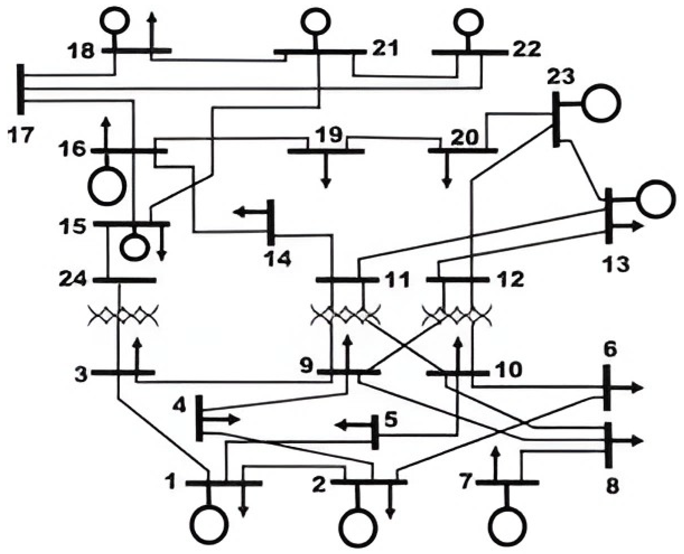
This study employs the IEEE 24-bus reliability test network to analyze the energy transition. The original system, detailed in Table 8, consists of 10 generation buses with conventional and hydroelectric technologies. Detailed data on generators, lines, and demand are provided in the annexes.
From the economic perspective, Table 9 specifies fixed costs by technology, while Table 10 details operational, fuel, and transmission variables.

Table 9.
Generation system costs
| Fuel | Technology | Cost [$/MWh] |
FOM [$/MW] |
|---|---|---|---|
| Oil | Combustion turbine | 10.22 | 409 |
| Steam turbine | - | - | |
| Coal | Steam turbine | 24.52 | 1154 |
| Water | Nuclear steam | 54.84 | 2117 |
| Water | Hydraulic turbine | 0.92 | 1535 |
| Wind | Wind turbine | 60 | 1477 |
Table 10.
Variable generation system costs
| Fuel | Technology | Cost [$/MWh] |
VOM [$/MWh] |
Fuel [$/MWh] |
ElecT [$/MWh] |
|---|---|---|---|---|---|
| Oil | Combustion turbine | 4.09 | 14.8 | 16.06 | 1.3 |
| Steam turbine | - | - | - | - | |
| Coal | Steam turbine | 3.07 | 40 | - | 0.8 |
| Water | Nuclear steam | 0.43 | 0.4 | - | - |
| Water | Hydraulic turbine | 0.003 | - | - | - |
| Wind | Wind turbine | 26.67 | - | - | - |
Figure 6.
IEEE 24-bus test system.
Complementarily, Table 11 quantifies carbon emissions and their associated costs, which define parameters for emission reduction by replacing fossil fuels with renewables.
4. Results Analysis
To evaluate the model, Phase 3 of William Newman’s method is implemented, applying the constraints and objective functions established in Phase 2. The analysis examines the impact of replacing fossil generation with renewable energy, demand-side management, and carbon-emission reduction on system operating costs and emissions.
The study develops three scenarios. The first, the base scenario, represents the current situation. The second, gradual transition, targets a 50% emission reduction over 20 years. Finally, the third, accelerated transition, targets a 75% reduction over 10 years.
4.1. Current-Situation Analysis
In the base scenario, the system operates without emission-reduction constraints or wind integration. Only conventional generation technologies are considered: coal, oil, and nuclear. The analysis evaluates the distribution of generation, carbon emissions, and associated costs.
Figure 7 shows the hourly evolution of generation by fuel type. Oil-based generation (red line) remains relatively constant, while nuclear (green line) exhibits greater variability. In contrast, coal-fired generation (blue line) experiences significant fluctuations.
Figure 8 presents the aggregated generation values by technology.
Oil (GenOil) shows the largest share, followed by nuclear (GenLW) and coal (GenCoal). Wind generation (GenW) is absent in this scenario.
Carbon dioxide (CO2) emissions by energy source are shown in Figure 9.
Oil and coal are the main emitters, with values exceeding 12,000 tons of CO2, reaching 12,000 tons for coal and 14,000 tons for oil. In contrast, nuclear and hydroelectric technologies do not produce direct emissions.
Finally, Figure 10 shows the relationship between the total generation cost and the cost of emissions.
The graph highlights an inverse correlation between energy generation costs and emission-related expenses. The quantitative analysis reveals a decreasing linear trend: as the emission cost rises from 0 to 600 $ annually, generation expenditure decreases from 90,000 to 32,000 $ in the same period.
This relationship suggests that reducing fossil-based generation and increasing renewable integration lowers system operating costs. However, it simultaneously increases expenses from emissions, creating a critical balance between environmental sustainability and economic feasibility.
4.2. Gradual Emission Reduction Analysis
The emission-reduction analysis is conducted over a 20-year horizon, considering a gradual increase in energy demand with a constant 20% expansion factor. Within this context, a structured transition process is implemented, in which conventional technologies progressively reduce their share, while renewable sources increase proportionally. These initial conditions form the operational basis for interpreting the results on generation, emissions, and costs presented below.
Figure 11 summarizes the system’s energy, environmental, and economic performance during the planning horizon. The annual generation chart shows a gradual reduction in oil and coal use, progressively replaced by hydro, wind, and, to a lesser extent, nuclear sources. This reconfiguration of the energy matrix results in sustained CO2 emission reductions, achieving a 50% decrease between years 9 and 20, as illustrated in the annual emission evolution chart. Economically, annual operating costs rise moderately due to the integration of renewable technologies. Additionally, annual emission costs steadily decline in terms of monetized environmental impact, demonstrating that the transition strategy is both technically and economically viable.
During the planning horizon, shown in Figure 12, electricity demand is continuously met despite the gradual phase-out of fossil sources. This balance is achieved through the progressive redesign of the energy mix, with a sustained increase in wind and hydro generation compensating for the reduction of coal and the eventual phase-out of oil in the final period. Nuclear generation maintains a steady and moderate contribution, serving as a backup technology in the transition.
The cumulative generation by source, described in Figure 13, shows that hydro accounts for 36% of the total, followed by oil at 28.6%, despite its progressive elimination in the final stages. Wind generation represents 16%, reflecting its growing incorporation into the energy mix. Coal and nuclear contribute 11.7% and 7.8%, respectively. This distribution highlights a system still partially dependent on conventional technologies, yet with notable progress toward renewable sources in terms of cumulative contribution.
The cumulative emissions balance, represented in Figure 14, shows that oil was responsible for 8,238 tCO2, marking the largest environmental impact, followed by coal with 4,563 tCO2, together totaling 12,802 tCO2. This concentration of emissions in two technologies fully justifies their progressive reduction and eventual retirement within the optimization model. The evidence confirms that the adopted strategy successfully guided the system toward a cleaner configuration without compromising coverage or technical operability.
4.3. Accelerated Emission Reduction Analysis
The accelerated transition scenario covers a 20-year period, considering a constant 20% increase in electricity demand. Under this scheme, an intensive substitution strategy is applied, in which conventional technologies rapidly decrease their share, favoring an accelerated penetration of renewable sources. This operational configuration provides the foundation to analyze system outcomes—focused on generation, emissions, and costs—with a 75% reduction achieved within the first 10 years.
Figure 15 illustrates an accelerated reconfiguration process of the system, where renewable sources, especially hydro and wind, gain early participation, while coal and oil use are drastically reduced starting in year 7. This technological substitution enables a 75% reduction in annual CO2 emissions by the end of year 10, as shown in the emission chart. Although generation costs show a sustained increase, emission-related costs decline significantly, evidencing an environmentally efficient transition with a moderate economic penalty.
During the accelerated transition, shown in Figure 16, electricity demand is continuously met despite the early retirement of conventional technologies. The gradual reduction of coal and the complete elimination of oil in the final year are offset by the steady growth of hydro generation, reinforced nuclear output, and greater wind participation.
This dynamic shows that, even under an accelerated substitution scenario, the system preserves operational stability and response capacity without compromising performance.
Meanwhile, the cumulative generation profile, detailed in Figure 17, indicates that, despite the short planning horizon, coal remains the dominant source with 35.9%, followed by nuclear at 20.2% and hydro at 19.1%. Oil generation falls significantly to 14.6%, while wind power reaches 10.2%, reflecting its gradual incorporation into the energy mix. These results highlight that, although the transition is accelerated, the operational inertia of conventional technologies continues to dominate cumulative contributions.
Cumulative emissions reach 6,171 tCO2, with coal accounting for 77% (4,742 tCO2) and oil the remaining 23% (1,430 tCO2), as shown in Figure 18. Compared to the base scenario, this represents a 75% reduction by the end of year 10, aligning with the model’s target. Therefore, the accelerated substitution strategy proves effective in reducing environmental impact over short periods without affecting system operation.
4.4. Phase 4: Evaluation and Validation of the Energy Transition
In Phase 4 of William Newman’s method, the results of the energy transition are evaluated and validated. This stage verifies the effectiveness of the strategies applied in Phase 3 by comparing proposed objectives with the outcomes obtained.
The analysis considers key metrics such as emission reduction, operating costs, and the share of renewable energy. These indicators make it possible to identify potential adjustments or improvements in the optimization model.
4.4.1. Emission Reduction Evaluation
The model set a target of reducing emissions by 50% through a gradual 20-year transition. However, the results show a reduction of only 15.38%, from 26,000 to 22,000 tons of CO2.
This outcome indicates that, although the applied strategy had a positive impact, it did not achieve the expected level of decarbonization. Therefore, additional strategies are needed to achieve a more effective reduction.
4.4.2. Cost Validation
The base scenario represents a system without emission restrictions and with predominant fossil generation. In this context, the annual generation cost reaches $90,000, while emission costs remain negligible at around $0. This reflects dependence on coal and oil, which are high operating-cost technologies without environmental penalties.
In contrast, the gradual transition scenario reduces fossil participation and increases renewable share. Here, generation costs decrease to $40,000 annually, but emissions costs reach $600 annually due to penalties. This shows that replacing polluting sources with renewables optimizes operating costs, although it introduces temporary financial impacts from environmental regulations.
The downward trend confirms that decarbonization entails initial costs but reduces expenses in the long term. Nevertheless, to ensure economic viability, complementary strategies are required—such as energy storage systems to guarantee operational stability and fiscal incentives to facilitate the progressive retirement of fossil assets.
5. Conclusions
The comprehensive analysis of the current power system revealed that coal- and oil-based thermoelectric generation remain the main contributors to greenhouse gas emissions. In the base scenario, these technologies account for 12,000 and 14,000 tons of CO2, respectively, underscoring the urgent need for an accelerated and structured energy transition.
The implementation of Mixed-Integer Linear Programming as a core optimization tool allowed for the evaluation of strategic pathways for decarbonization. Under the gradual transition scenario, the integration of wind and hydro power reduced oil-related emissions to 10,000 tons, while coal remained steady at 12,000 tons, achieving an overall reduction of 15.38%. Although this demonstrates tangible progress, the results fell short of the targeted 50% reduction, highlighting that incremental renewable integration alone is insufficient to reach ambitious climate goals.
The accelerated transition scenario, by contrast, confirmed the technical feasibility of achieving a 75% emission reduction within 10 years. This was made possible through the rapid phase-out of fossil-based generation, combined with significant renewable penetration and the deployment of energy storage systems. However, the results also revealed higher operational costs during the early years, emphasizing the economic trade-offs that policymakers and system operators must address.
From an economic perspective, the study showed that decarbonization not only reduces long-term operational costs but also enhances system resilience against volatility in fossil fuel markets. Nevertheless, short-term financial penalties associated with carbon pricing and renewable integration costs require complementary measures. These include fiscal incentives, regulatory frameworks that accelerate the retirement of carbon-intensive assets, and investments in grid flexibility and storage technologies.
Technically, the research highlights the importance of balancing renewable penetration with reliability requirements. Demand response programs, hybrid renewable energy systems, and binary operation of generation units proved essential to maintaining supply security and system stability throughout the transition.
In summary, the proposed framework validates that a sustainable and economically viable decarbonization of the power sector is achievable under specific conditions. Success requires a combination of four pillars: (i) accelerated renewable integration, (ii) large-scale deployment of storage systems, (iii) active demand-side participation, and (iv) strong regulatory and fiscal policies. These elements together ensure that emission reduction targets can be realistically met without compromising energy security or economic competitiveness. Beyond its immediate findings, the framework developed is replicable and adaptable, offering a practical roadmap for other power systems facing similar decarbonization challenges.
Abbreviations
| ARMA | AutoRegressive Moving Average |
| BRP | Balance Responsible Party |
| CELEC EP | Corporación Eléctrica del Ecuador |
| CO2 | Carbon Dioxide |
| DOD | Depth of Discharge |
| DR | Demand Response |
| DSO | Distribution System Operator |
| ECEC | Electric System Carbon Emissions |
| EECC | Expected Cost of Unserved Energy |
| EGSC | Electric System Generation Cost |
| ELRC | Load Response Cost |
| EMF | Electromotive Force |
| HRES | Hybrid Renewable Energy Systems |
| HVAC | Heating, Ventilation, and Air Conditioning |
| IEEE | Institute of Electrical and Electronics Engineers |
| MCI | Internal Combustion Engine |
| MILP | Mixed-Integer Linear Programming |
| MVA | Megavolt-ampere |
| MW | Megawatt |
| MWh | Megawatt-hour |
| NOCT | Nominal Operating Cell Temperature |
| PLM | Programación Lineal Mixta |
| RD | Demand Response |
| SEP | Power Electric System |
| SOC | State of Charge |
| TOU | Time of Use |
| TSO | Transmission System Operator |
Appendix A. Technical Data of the Test System
Table A.1.
Technical data of generating units
| Unit # | Node | Pmaxi [MW] |
Pmini [MW] |
R+i [MW] |
R-i [MW] |
RUi [MW/h] |
RDi [MW/h] |
UT [h] |
DT [h] |
|---|---|---|---|---|---|---|---|---|---|
| 1 | 1 | 152 | 30.4 | 40 | 40 | 120 | 120 | 8 | 4 |
| 2 | 2 | 152 | 30.4 | 40 | 40 | 120 | 120 | 8 | 4 |
| 3 | 7 | 350 | 75 | 70 | 70 | 350 | 350 | 8 | 8 |
| 4 | 13 | 591 | 206.85 | 180 | 180 | 240 | 240 | 12 | 10 |
| 5 | 15 | 60 | 12 | 60 | 60 | 60 | 60 | 4 | 2 |
| 6 | 15 | 155 | 54.25 | 30 | 30 | 155 | 155 | 8 | 8 |
| 7 | 16 | 155 | 54.25 | 30 | 30 | 155 | 155 | 8 | 8 |
| 8 | 18 | 400 | 100 | 0 | 0 | 280 | 280 | 1 | 1 |
| 9 | 21 | 400 | 100 | 0 | 0 | 280 | 280 | 1 | 1 |
| 10 | 22 | 300 | 300 | 0 | 0 | 300 | 300 | 0 | 0 |
| 11 | 23 | 310 | 108.5 | 60 | 60 | 180 | 180 | 8 | 8 |
| 12 | 23 | 350 | 140 | 40 | 40 | 240 | 240 | 8 | 8 |
Table A.2.
Reactance and capacity of transmission lines
| From | To | Reactance [p.u.] |
Capacity [MVA] |
From | To | Reactance [p.u.] |
Capacity [MVA] |
|---|---|---|---|---|---|---|---|
| 1 | 2 | 0.0146 | 175 | 11 | 13 | 0.0488 | 500 |
| 1 | 3 | 0.2253 | 175 | 11 | 14 | 0.0426 | 500 |
| 1 | 5 | 0.0907 | 350 | 12 | 13 | 0.0488 | 500 |
| 2 | 4 | 0.1356 | 175 | 12 | 23 | 0.0985 | 500 |
| 2 | 6 | 0.2050 | 175 | 13 | 23 | 0.0884 | 500 |
| 3 | 24 | 0.0840 | 400 | 14 | 16 | 0.0110 | 500 |
| 4 | 9 | 0.2550 | 400 | 15 | 16 | 0.0172 | 500 |
| 5 | 10 | 0.0940 | 350 | 16 | 17 | 0.0920 | 500 |
| 6 | 10 | 0.0642 | 350 | 16 | 21 | 0.0529 | 500 |
| 7 | 8 | 0.0652 | 250 | 17 | 22 | 0.0233 | 500 |
| 8 | 9 | 0.1762 | 250 | 18 | 21 | 0.0669 | 500 |
| 9 | 10 | 0.0840 | 400 | 19 | 20 | 0.0203 | 1000 |
| 10 | 11 | 0.0840 | 400 | 22 | 23 | 0.0355 | 500 |
| 10 | 12 | 0.0840 | 400 | 21 | 22 | 0.0692 | 500 |
Table A.3.
Load profile
| Hour | System demand [MW] |
Hour | System demand [MW] |
|---|---|---|---|
| 1 | 1775.835 | 13 | 2517.975 |
| 2 | 1669.815 | 14 | 2517.975 |
| 3 | 1590.3 | 15 | 2464.965 |
| 4 | 1563.795 | 16 | 2464.965 |
| 5 | 1563.795 | 17 | 2623.995 |
| 6 | 1590.3 | 18 | 2650.5 |
| 7 | 1961.37 | 19 | 2650.5 |
| 8 | 2279.43 | 20 | 2544.48 |
| 9 | 2517.975 | 21 | 2411.995 |
| 10 | 2544.48 | 22 | 2199.915 |
| 11 | 2544.48 | 23 | 1934.865 |
| 12 | 2517.975 | 24 | 1669.815 |
Table A.4.
Node locations and distribution of total system demand
| Load # | Node | % of system load | Load # | Node | % of system load |
|---|---|---|---|---|---|
| 1 | 1 | 3.8 | 10 | 10 | 6.8 |
| 2 | 2 | 3.4 | 11 | 13 | 9.3 |
| 3 | 3 | 6.3 | 12 | 14 | 6.8 |
| 4 | 4 | 2.6 | 13 | 15 | 11.1 |
| 5 | 5 | 2.5 | 14 | 16 | 3.5 |
| 6 | 6 | 4.8 | 15 | 18 | 11.7 |
| 7 | 7 | 4.4 | 16 | 19 | 6.4 |
| 8 | 8 | 6.0 | 17 | 20 | 4.5 |
| 9 | 9 | 6.1 |
References
- Fu, P.; Pudjianto, D.; Zhang, X.; Strbac, G. Evaluating Strategies for Decarbonising the Transport Sector in Great Britain. In Proceedings of the 2019 IEEE Milan PowerTech. IEEE, 2019, pp. 1–6. [CrossRef]
- Herenčić, L.; Melnjak, M.; Capuder, T.; Andročec, I.; Rajšl, I. Techno-economic and environmental assessment of energy vectors in decarbonization of energy islands. Energy Conversion and Management 2021, 236, 114064. [Google Scholar] [CrossRef]
- Shen, X.; Li, S.; Li, H. Large-scale Offshore Wind Farm Electrical Collector System Planning: A Mixed-Integer Linear Programming Approach. In Proceedings of the 2021 IEEE 5th Conference on Energy Internet and Energy System Integration (EI2). IEEE, 2021, pp. 1248–1253. [CrossRef]
- Petrelli, M.; Fioriti, D.; Berizzi, A.; Poli, D. Multi-Year Planning of a Rural Microgrid Considering Storage Degradation. IEEE Transactions on Power Systems 2021, 36, 1459–1469. [Google Scholar] [CrossRef]
- Bornand, B.; Girardin, L.; Belfiore, F.; Robineau, J.L.; Bottallo, S.; Maréchal, F. Investment Planning Methodology for Complex Urban Energy Systems Applied to a Hospital Site. Frontiers in Energy Research 2020, 8. [Google Scholar] [CrossRef]
- Tran, T.H.; Mao, Y.; Siebers, P.O. Optimising Decarbonisation Investment for Firms towards Environmental Sustainability. Sustainability 2019, 11, 5718. [Google Scholar] [CrossRef]
- Bonthu, R.K.; Aguilera, R.P.; Pham, H.; Phung, M.D.; Ha, Q.P. Energy Cost Optimization in Microgrids Using Model Predictive Control and Mixed Integer Linear Programming. In Proceedings of the 2019 IEEE International Conference on Industrial Technology (ICIT). IEEE, 2019, pp. 1113–1118. [CrossRef]
- Uberti, V.A.; Adeyanju, O.M.; Bernardon, D.P.; Abaide, A.R.; Pereira, P.R.; Prade, L.R. Linear Programming Applied to Expansion Planning of Power Transmission System. In Proceedings of the 2019 IEEE PES Innovative Smart Grid Technologies Conference - Latin America (ISGT Latin America). IEEE, 2019, pp. 1–4. [CrossRef]
- dos Santos, C.; Rider, M.J.; Lyra, C. Optimized Integration of a Set of Small Renewable Sources Into a Bulk Power System. IEEE Transactions on Power Systems 2021, 36, 248–260. [Google Scholar] [CrossRef]
- Weber, C.; Furtwängler, C. Managing combined power and heat portfolios in sequential spot power markets under uncertainty. SSRN Electronic Journal 2020. [Google Scholar] [CrossRef]
- El Sayed, A.; Poyrazoglu, G.; Ahmed, E.E.E. Capacity Planning for Forming Sustainable and Cost-Effective Nanogrids. In Proceedings of the 2023 13th International Conference on Power, Energy and Electrical Engineering (CPEEE). IEEE, 2023, pp. 217–222. [CrossRef]
- Pinzon, J.A.; Vergara, P.P.; da Silva, L.C.P.; Rider, M.J. Optimal Management of Energy Consumption and Comfort for Smart Buildings Operating in a Microgrid. IEEE Transactions on Smart Grid 2019, 10, 3236–3247. [Google Scholar] [CrossRef]
- Melgar-Dominguez, O.D.; Pourakbari-Kasmaei, M.; Mantovani, J.R.S. Robust Short-Term Electrical Distribution Network Planning Considering Simultaneous Allocation of Renewable Energy Sources and Energy Storage Systems. In Robust Optimal Planning and Operation of Electrical Energy Systems; Springer International Publishing: Cham, 2019; pp. 145–175. [Google Scholar] [CrossRef]
- Hasnaoui, A.; Omari, A.; Azzouz, Z.E. Optimization of Building Energy based on Mixed Integer Linear Programming. In Proceedings of the 2022 2nd International Conference on Advanced Electrical Engineering (ICAEE). IEEE, 2022, pp. 1–6. [CrossRef]
- Silva, J.A.A.; López, J.C.; Arias, N.B.; Rider, M.J.; da Silva, L.C.P. An optimal stochastic energy management system for resilient microgrids. Applied Energy 2021, 300, 117435. [Google Scholar] [CrossRef]
- Cerchio, M.; Gullì, F.; Repetto, M.; Sanfilippo, A. Hybrid Energy Network Management: Simulation and Optimisation of Large Scale PV Coupled with Hydrogen Generation. Electronics 2020, 9, 1734. [Google Scholar] [CrossRef]
- Pombo, D.V.; Martinez-Rico, J.; Carrion, M.; Cañas-Carreton, M. A Computationally Efficient Formulation for a Flexibility Enabling Generation Expansion Planning. IEEE Transactions on Smart Grid 2023, 14, 2723–2733. [Google Scholar] [CrossRef]
- Basto-Gil, J.; Maldonado-Cardenas, A.; Montoya, O. Optimal Selection and Integration of Batteries and Renewable Generators in DC Distribution Systems through a Mixed-Integer Convex Formulation. Electronics 2022, 11, 3139. [Google Scholar] [CrossRef]
- Weimann, L.; Gabrielli, P.; Boldrini, A.; Kramer, G.J.; Gazzani, M. On the role of H2 storage and conversion for wind power production in the Netherlands. In Proceedings of the Computer Aided Chemical Engineering, 2019, pp. 1627–1632. [CrossRef]
- Neumann, F.; Brown, T. Heuristics for Transmission Expansion Planning in Low-Carbon Energy System Models. In Proceedings of the 2019 16th International Conference on the European Energy Market (EEM). IEEE, 2019, pp. 1–8. [CrossRef]
- Li, C.; Conejo, A.J.; Liu, P.; Omell, B.P.; Siirola, J.D.; Grossmann, I.E. Mixed-integer linear programming models and algorithms for generation and transmission expansion planning of power systems. European Journal of Operational Research 2022, 297, 1071–1082. [Google Scholar] [CrossRef]
- Mallégol, A.; Khannoussi, A.; Mohammadi, M.; Lacarrière, B.; Meyer, P. Handling Non-Linearities in Modelling the Optimal Design and Operation of a Multi-Energy System. Mathematics 2023, 11, 4855. [Google Scholar] [CrossRef]
- Fleschutz, M.; Bohlayer, M.; Braun, M.; Murphy, M.D. Demand Response Analysis Framework (DRAF): An Open-Source Multi-Objective Decision Support Tool for Decarbonizing Local Multi-Energy Systems. Sustainability 2022, 14, 8025. [Google Scholar] [CrossRef]
- Bianco, V.; Driha, O.M.; Sevilla-Jiménez, M. Effects of renewables deployment in the Spanish electricity generation sector. Utilities Policy 2019, 56, 72–81. [Google Scholar] [CrossRef]
- Dyson, M. Sharpening Focus on a Global Low-Carbon Future. Joule 2017, 1, 15–17. [Google Scholar] [CrossRef]
- Farnsworth, A.; Gençer, E. Highlighting regional decarbonization challenges with novel capacity expansion model. Cleaner Energy Systems 2023, 5, 100078. [Google Scholar] [CrossRef]
- Sari, A.; Akkaya, M. Contribution of Renewable Energy Potential to Sustainable Employment. Procedia - Social and Behavioral Sciences 2016, 229, 316–325. [Google Scholar] [CrossRef]
- Mercure, J.F.; Pollitt, H.; Bassi, A.M.; Viñuales, J.E.; Edwards, N.R. Modelling complex systems of heterogeneous agents to better design sustainability transitions policy. Global Environmental Change 2016, 37, 102–115. [Google Scholar] [CrossRef]
- Erdiwansyah.; Mahidin.; Husin, H.; Nasaruddin.; Zaki, M.; Muhibbuddin. A critical review of the integration of renewable energy sources with various technologies. Protection and Control of Modern Power Systems 2021, 6. [CrossRef]
- Agencia de Regulación y Control de Energía y Recursos Naturales No Renovables. Estadística Anual y Multianual del Sector Eléctrico Ecuatoriano. Technical report, 2023.
- Chiavenato, I.; Sapiro, A. Planeación Estratégica. Fundamentos y aplicaciones; McGRAW-HILL, 2017.
- Mintzberg, H.; Ahlstrand, B.; Lampel, J. Safari a la estrategia. Una visita guiada por la jungla del management estratégico; Granica, 2024.
- Secretaría Nacional de Planificación y Desarrollo. Plan Nacional de Desarrollo 2017-2021-Toda una Vida. Technical report, 2017.
- Franke, G.; Schneider, M.; Weitzel, T.; Rinderknecht, S. Stochastic Optimization Model for Energy Management of a Hybrid Microgrid using Mixed Integer Linear Programming. IFAC-PapersOnLine 2020, 53, 12948–12955. [Google Scholar] [CrossRef]
- Pardo, R.A.; López-Lezama, J.M. Power system restoration using a mixed integer linear programming model. Información Tecnológica 2021, 31, 147–158. [Google Scholar] [CrossRef]
- Cosic, A.; Stadler, M.; Mansoor, M.; Zellinger, M. Mixed-integer linear programming based optimization strategies for renewable energy communities. Energy 2021, 237, 121559. [Google Scholar] [CrossRef]
- Rueda Sosa, J.R. Diseño de un modelo de planeación estratégica soportado en el sistema gerencial de Kaplan y Norton, aplicable a las mipymes de reciente creación originadas como proyectos formales de emprendimiento en Bogotá. Master’s thesis, Universidad Nacional de Colombia, 2014.
- Páez, B. Análisis de los escenarios respecto al crecimiento de las energías no convencionales en el Ecuador para el año 2030. Master’s thesis, Escuela Politécnica Nacional, 2023.
- Adefarati, T.; Bansal, R.C. Integration of renewable distributed generators into the distribution system: A review. IET Renewable Power Generation 2016, 10, 873–884. [Google Scholar] [CrossRef]
- Haegel, N.; Kurtz, S. Global Progress Toward Renewable Electricity: Tracking the Role of Solar. IEEE Journal of Photovoltaics 2021, 11, 1335–1342. [Google Scholar] [CrossRef]
- Kuma, J.; Ashley, D. Runoff estimates into the Weija reservoir and its implications for water supply to the Accra area, Ghana. Journal of Urban and Environmental Engineering 2013, 2, 33–40. [Google Scholar] [CrossRef]
- Chen, Z.; Wang, Y.; Zhang, X. Energy and exergy analyses of S–CO2 coal-fired power plant with reheating processes. Energy 2020, 211, 118651. [Google Scholar] [CrossRef]
- CENACE. Informe Anual CENACE. Technical report, 2018.
- Ostman, F.; Toivonen, H.T. Adaptive Cylinder Balancing of Internal Combustion Engines. IEEE Transactions on Control Systems Technology 2011, 19, 782–791. [Google Scholar] [CrossRef]
- Pereira, F.; Silva, C. Combustion of Emulsions in Internal Combustion Engines and Reduction of Pollutant Emissions in Isolated Electricity Systems. Energies 2022, 15, 8053. [Google Scholar] [CrossRef]
- Kumar, R.R.; Pandey, K.M. Static Structural and Modal Analysis of Gas Turbine Blade. IOP Conference Series: Materials Science and Engineering 2017, 225, 012102. [Google Scholar] [CrossRef]
- Tukur, N.; Osigwe, E.O. A model for booster station matching of gas turbine and gas compressor power under different ambient conditions. Heliyon 2021, 7, e07222. [Google Scholar] [CrossRef]
- Milovanović, Z.N.; Papić, L.R.; Milovanović, S.Z.; Janičić Milovanović, V.Z.; Dumonjić-Milovanović, S.R.; Branković, D.L. Qualitative analysis in the reliability assessment of the steam turbine plant. In The Handbook of Reliability, Maintenance, and System Safety through Mathematical Modeling; Elsevier, 2021; pp. 179–313. [CrossRef]
- Lee, D.S.; Kim, B.G.; Kwon, S.K. Efficient Depth Data Coding Method Based on Plane Modeling for Intra Prediction. IEEE Access 2021, 9, 29153–29164. [Google Scholar] [CrossRef]
- Plazas-Niño, F.A.; Ortiz-Pimiento, N.R.; Montes-Páez, E.G. National energy system optimization modelling for decarbonization pathways analysis: A systematic literature review. Renewable and Sustainable Energy Reviews 2022, 162, 112406. [Google Scholar] [CrossRef]
- Urrutia Azcona, K.; Stendorf Sorensen, S.; Molina Costa, P.; Flores Abascal, I. Smart zero carbon city: key factors towards smart urban decarbonization. DYNA 2019, 94, 676–683. [Google Scholar] [CrossRef]
- Howard-Grenville, J.; Buckle, S.J.; Hoskins, B.J.; George, G. Climate Change and Management. Academy of Management Journal 2014, 57, 615–623. [Google Scholar] [CrossRef]
- Mirzaesmaeeli, H.; Elkamel, A.; Douglas, P.L.; Croiset, E.; Gupta, M. A multi-period optimization model for energy planning with CO2 emission consideration. Journal of Environmental Management 2010, 91, 1063–1070. [Google Scholar] [CrossRef]
- Alstone, P.; Gershenson, D.; Kammen, D.M. Decentralized energy systems for clean electricity access. Nature Climate Change 2015, 5, 305–314. [Google Scholar] [CrossRef]
- Hou, J.; Guo, J.; Liu, J. An economic load dispatch of wind-thermal power system by using virtual power plants. In Proceedings of the Chinese Control Conference, 2016, pp. 8704–8709. [CrossRef]
- Cao, C.; Xie, J.; Yue, D.; Zhao, J.; Xiao, Y.; Wang, L. A distributed gradient algorithm based economic dispatch strategy for virtual power plant. In Proceedings of the Chinese Control Conference, 2016, pp. 7826–7831. [CrossRef]
- Ahmad, J.; et al. Techno economic analysis of a wind-photovoltaic-biomass hybrid renewable energy system for rural electrification: A case study of Kallar Kahar. Energy 2018, 148, 208–234. [Google Scholar] [CrossRef]
- Mehrpooya, M.; Mohammadi, M.; Ahmadi, E. Techno-economic-environmental study of hybrid power supply system: A case study in Iran. Sustainable Energy Technologies and Assessments 2018, 25, 1–10. [Google Scholar] [CrossRef]
- Escobar, G.B.A. Óptima Respuesta a la Demanda y Despacho Económico de Energía Eléctrica en Micro Redes Basados en Árboles de Decisión Estocástica. Master’s thesis, Universidad Politécnica Salesiana, 2018.
- Moyón, R.A.F. Planeación de Despacho Óptimo de Plantas Virtuales de Generación en Sistemas Eléctricos de Potencia mediante Flujos Óptimos de Potencia AC. Master’s thesis, Universidad Politécnica Salesiana, 2020.
- Hosseinalizadeh, R.; Shakouri, H.; Amalnick, M.S.; Taghipour, P. Economic sizing of a hybrid (PV–WT–FC) renewable energy system (HRES) for stand-alone usages by an optimization-simulation model: Case study of Iran. Renewable and Sustainable Energy Reviews 2016, 54, 139–150. [Google Scholar] [CrossRef]
- Al-Shamma’a, A.A.; Alturki, F.A.; Farh, H.M.H. Techno-economic assessment for energy transition from diesel-based to hybrid energy system-based off-grids in Saudi Arabia. Energy Transitions 2020, 4, 31–43. [Google Scholar] [CrossRef]
- Lao, C.; Chungpaibulpatana, S. Techno-economic analysis of hybrid system for rural electrification in Cambodia. Energy Procedia 2017, 138, 524–529. [Google Scholar] [CrossRef]
- Carlos, B.; Félix, G.T.; Miguel, A.R. Model predictive Control of Microgrids; 2019.
- Murnane, M.; Ghazel, A. A Closer Look at State of Charge (SOC) and State of Health (SOH) Estimation Techniques for Batteries. Technical report, 2017.
- Vahid-Ghavidel, M.; Javadi, M.S.; Gough, M.; Santos, S.F.; Shafie-Khah, M.; Catalão, J.P.S. Demand response programs in multi-energy systems: A review. Energies 2020, 13, 1–17. [Google Scholar] [CrossRef]
- Ko, W.; Vettikalladi, H.; Song, S.H.; Choi, H.J. Implementation of a demand-side management solution for South Korea’s demand response program. Applied Sciences 2020, 10. [Google Scholar] [CrossRef]
- Ma, Z.; Billanes, J.D.; Jørgensen, B.N. Aggregation potentials for buildings-Business models of demand response and virtual power plants. Energies 2017, 10. [Google Scholar] [CrossRef]
- Lamprinos, I.; Hatziargyriou, N.D.; Kokos, I.; Dimeas, A.D. Making Demand Response a Reality in Europe: Policy, Regulations, and Deployment Status. IEEE Communications Magazine 2016, 54, 108–113. [Google Scholar] [CrossRef]
- Khoo, W.C.; Teh, J.; Lai, C.M. Integration of Wind and Demand Response for Optimum Generation Reliability, Cost and Carbon Emission. IEEE Access 2020, 8, 183606–183618. [Google Scholar] [CrossRef]
Figure 1.
William Newman model applied to the power system
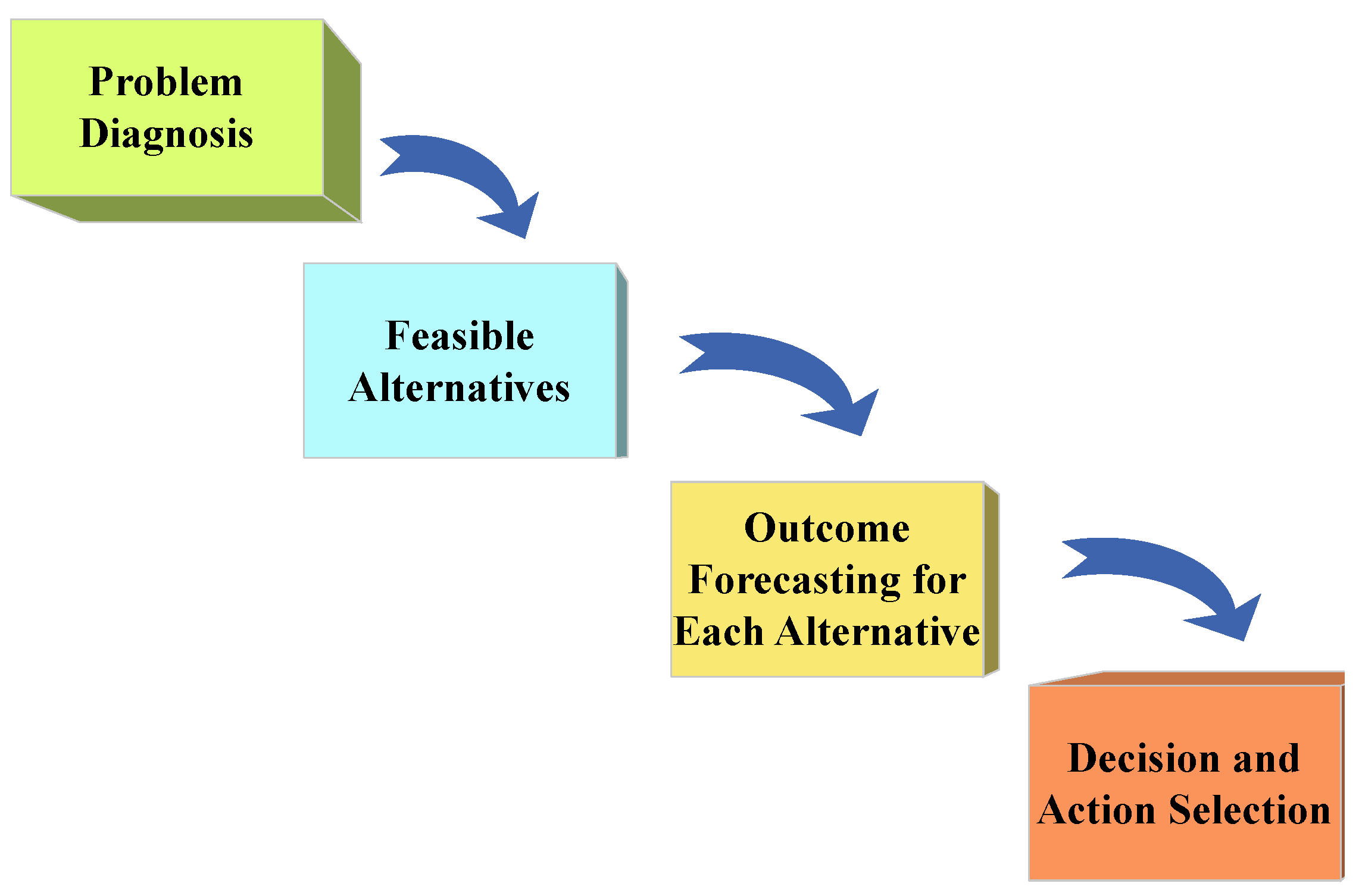
Figure 2.
Decarbonization processes
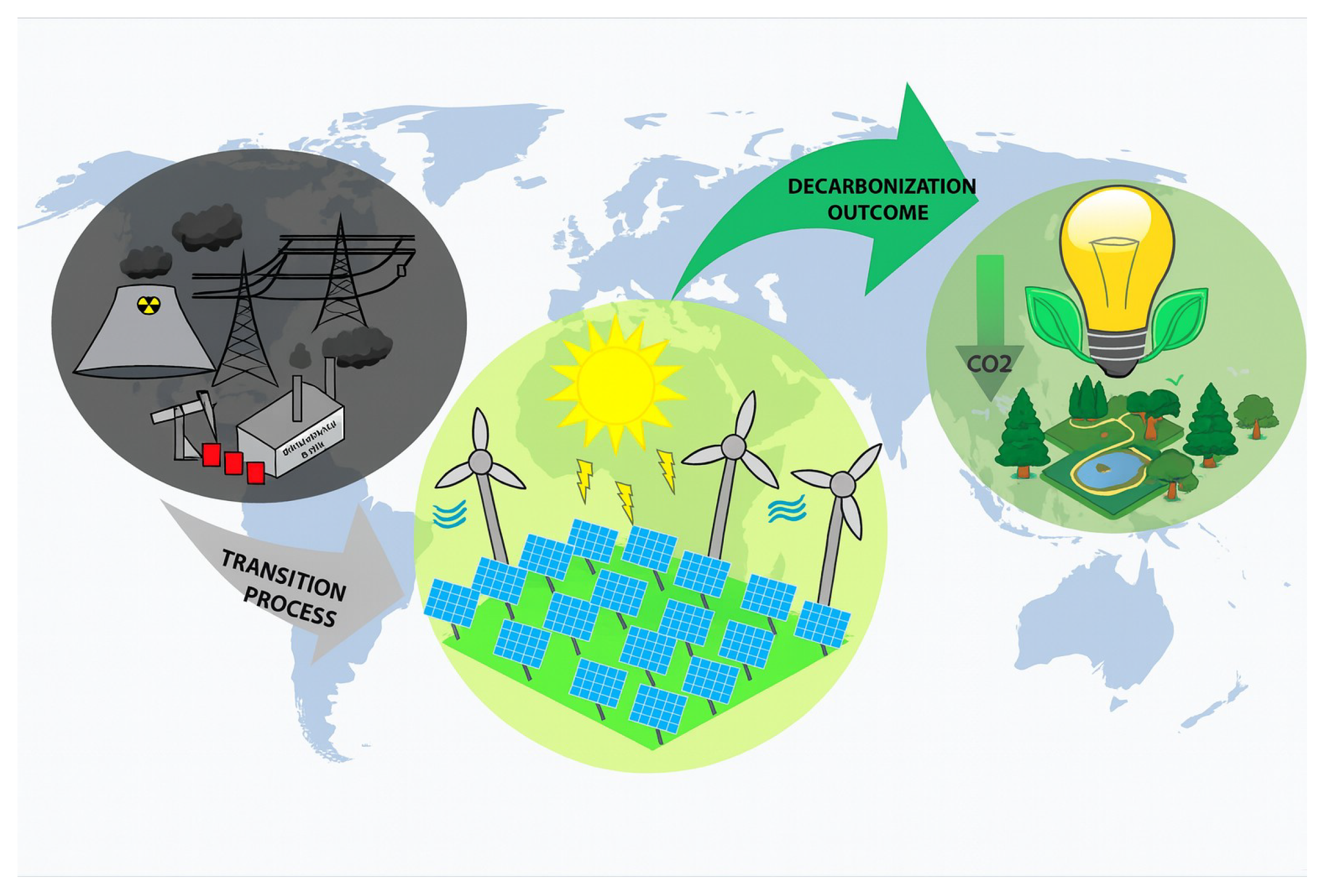
Figure 3.
24-hour demand variability horizon
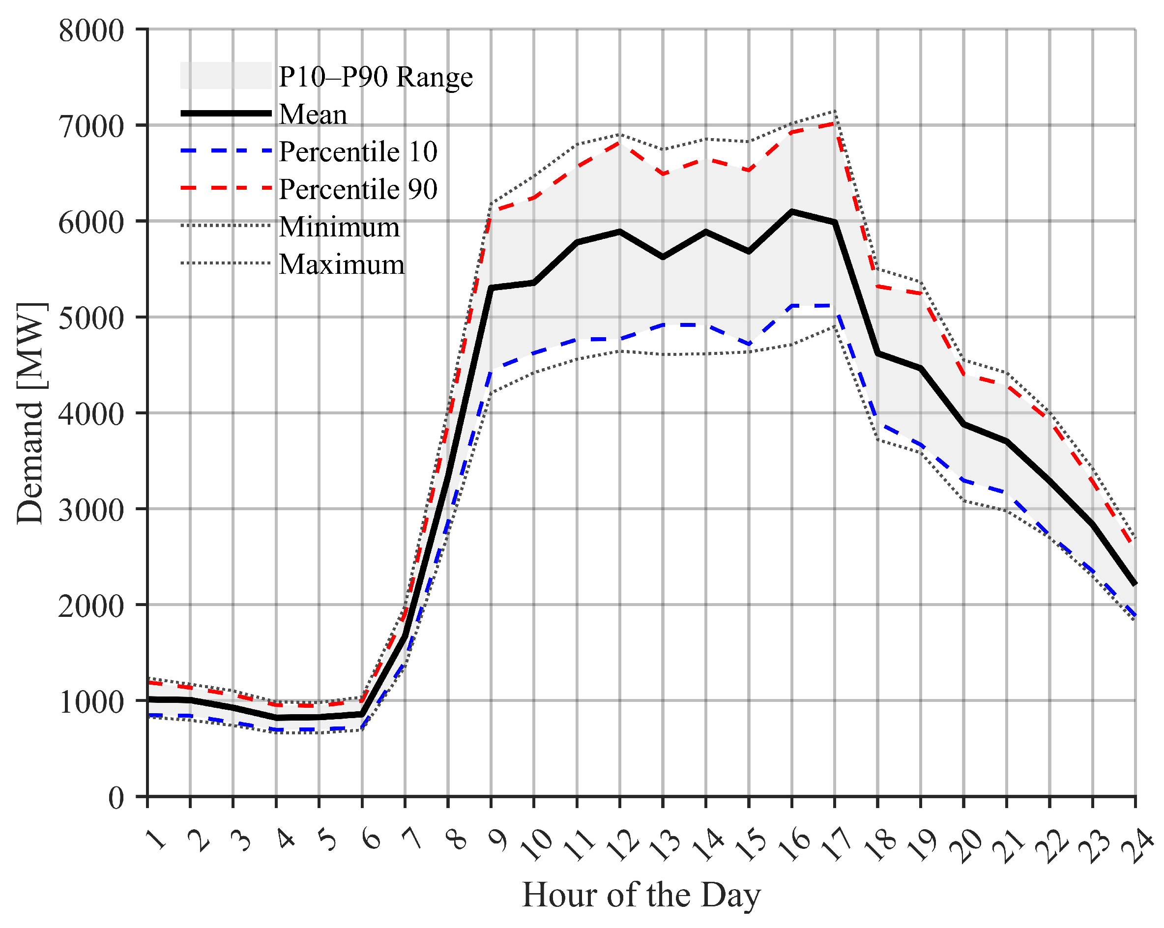
Figure 4.
10-year demand variability horizon
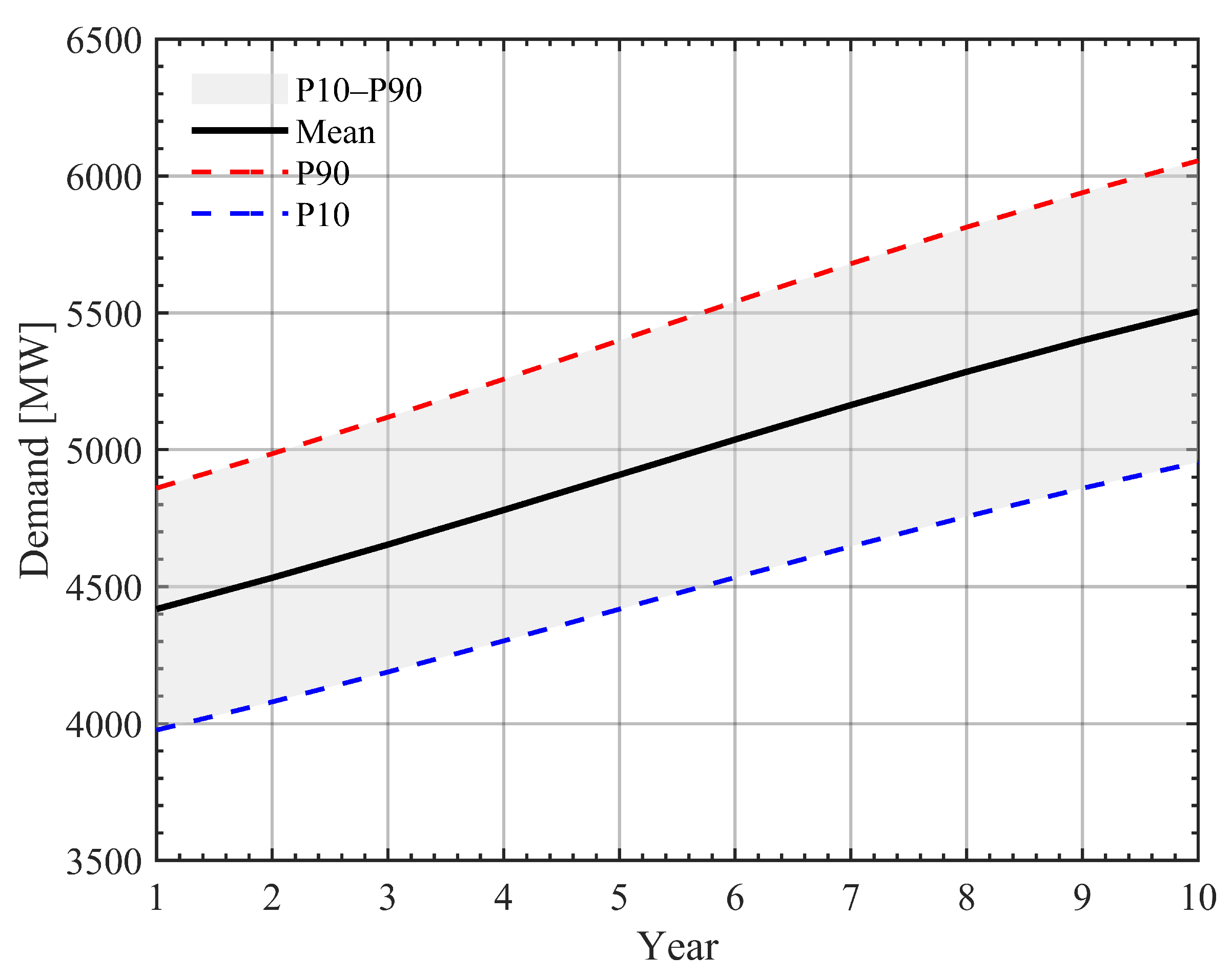
Figure 5.
20-year demand variability horizon
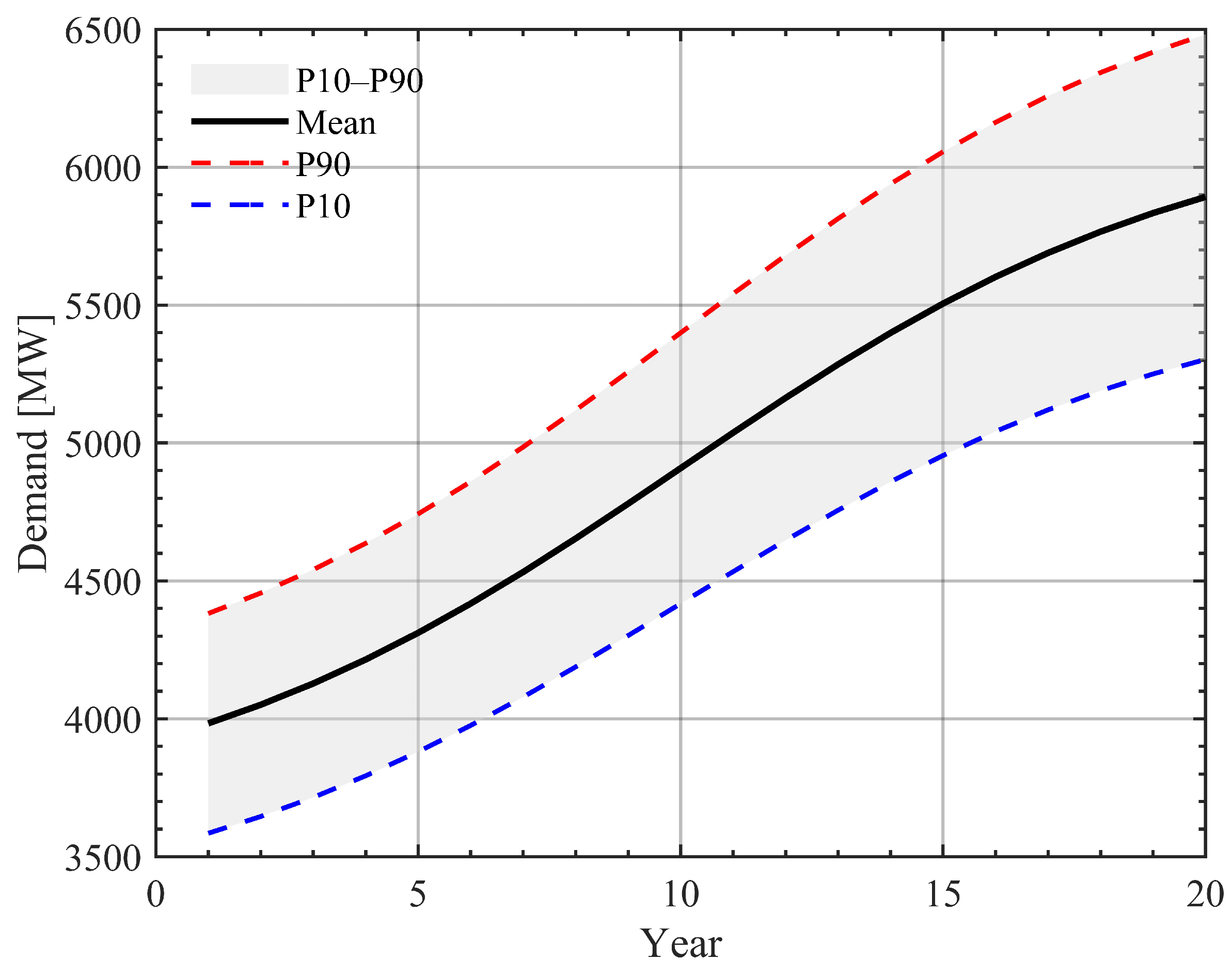
Figure 7.
Generation behavior — base scenario
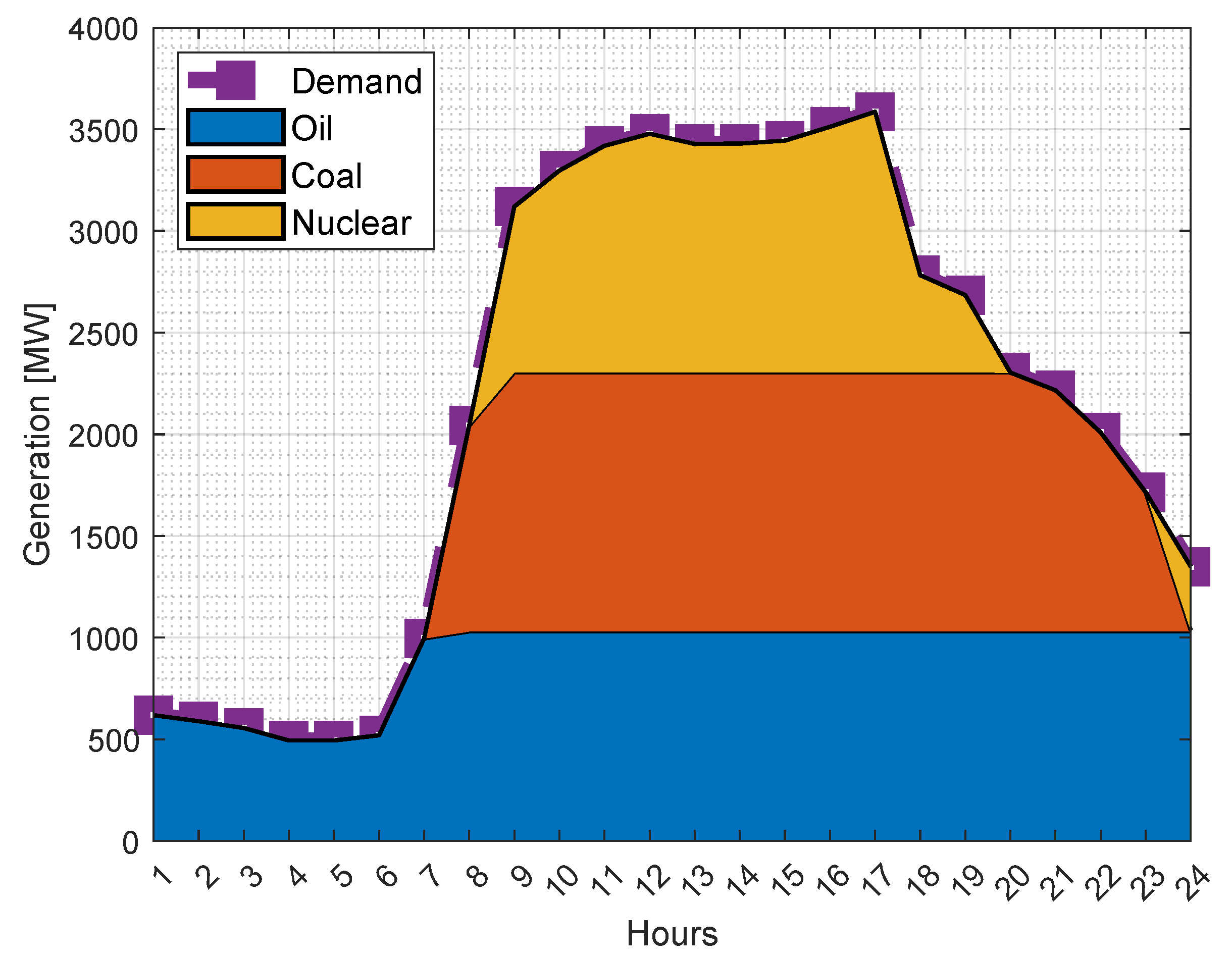
Figure 8.
Total power by technology — base scenario
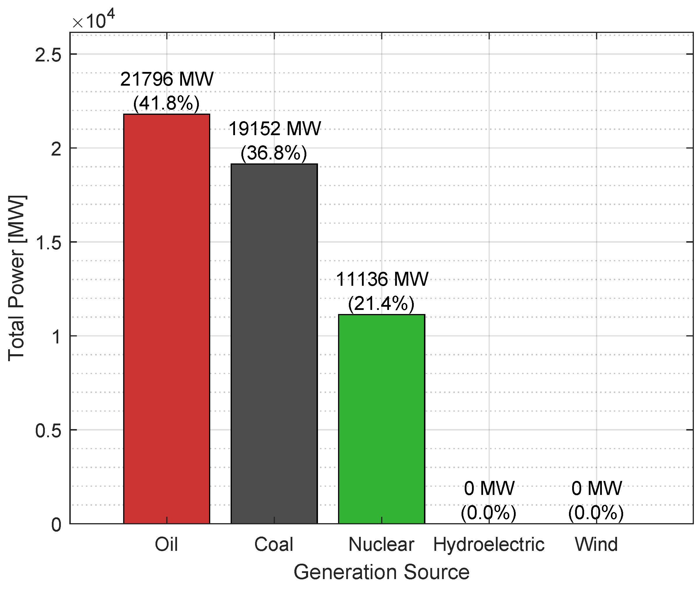
Figure 9.
Total emissions by technology — base scenario
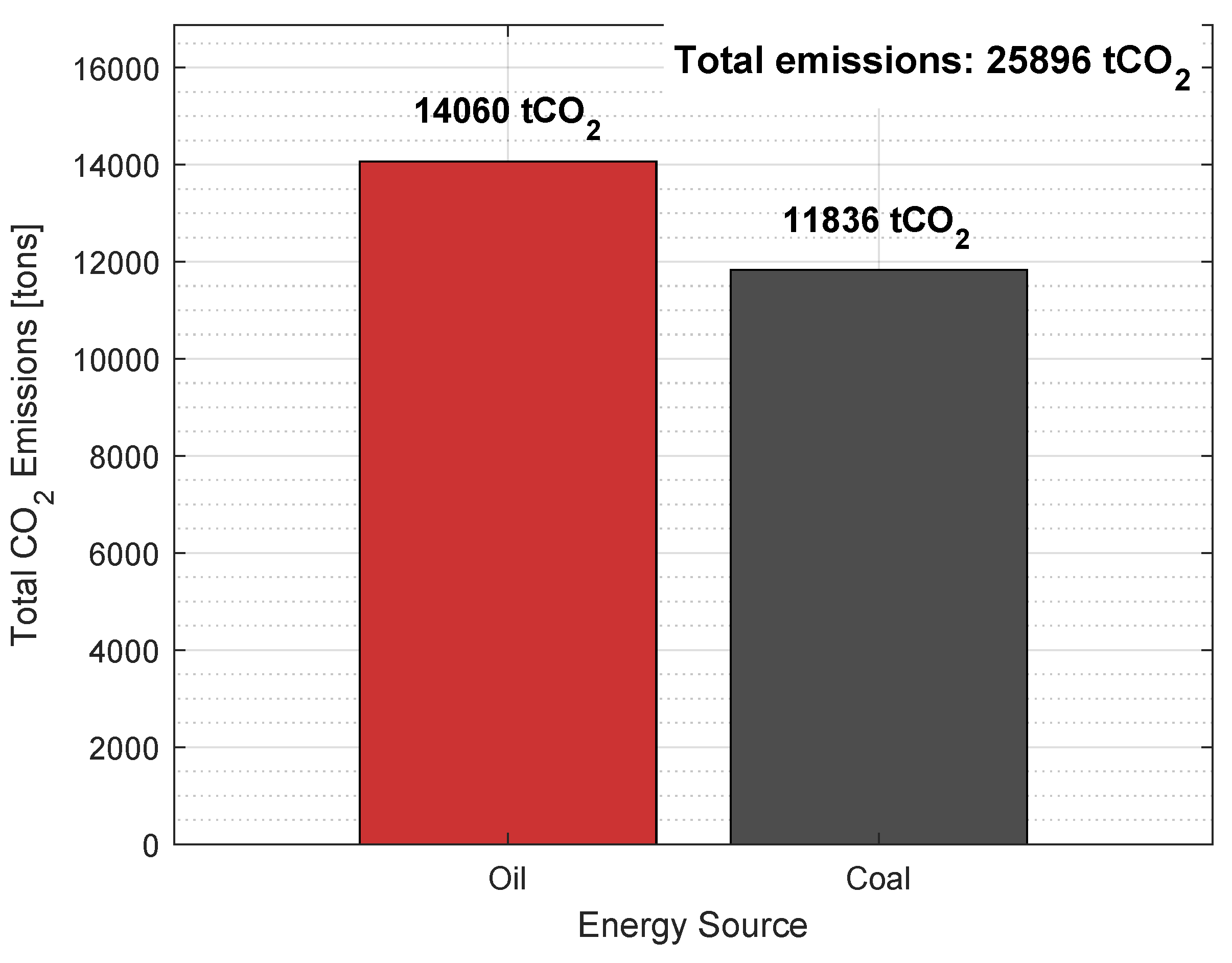
Figure 10.
Generation cost vs. emission cost — base scenario
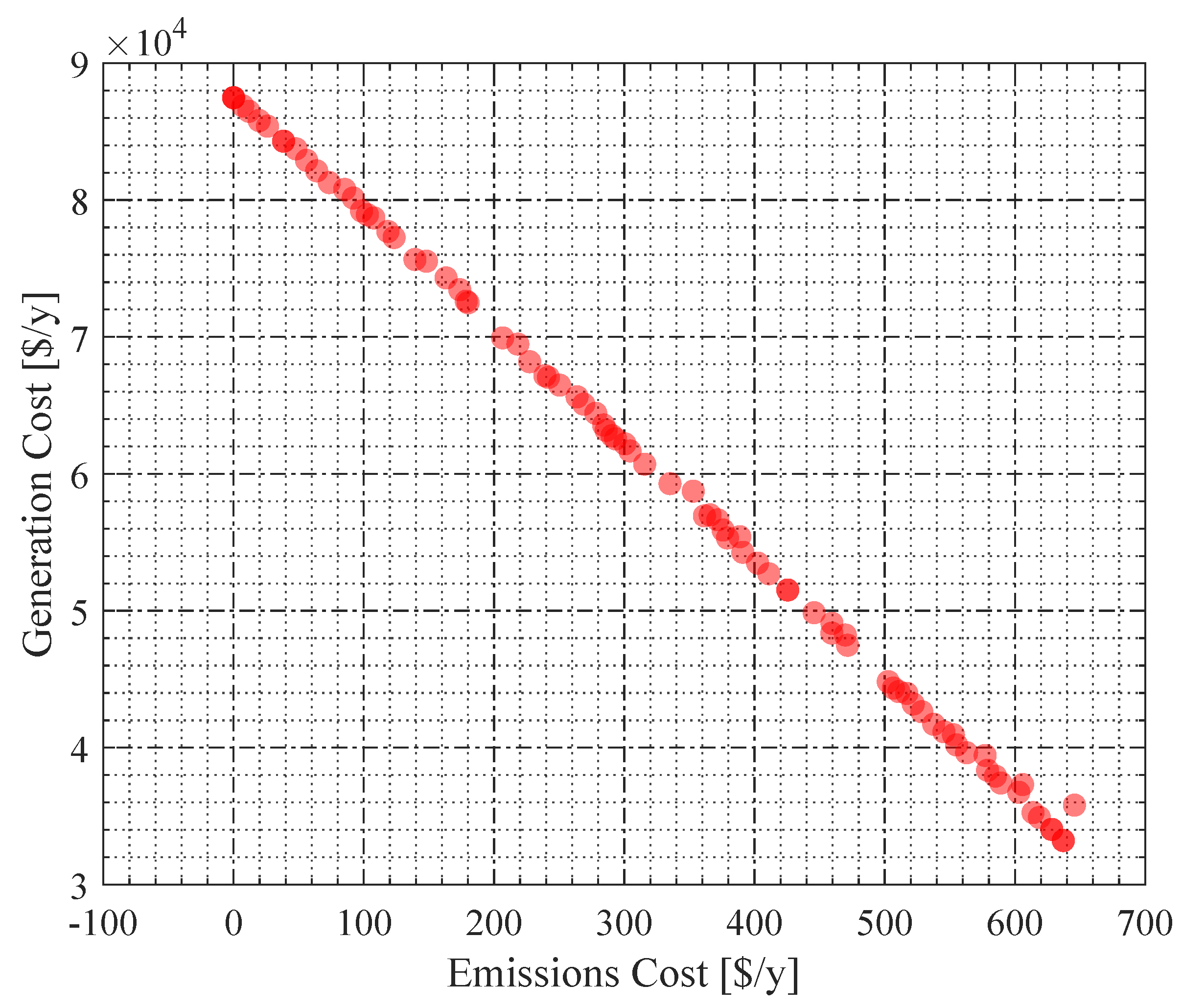
Figure 11.
Energy, environmental, and economic performance of the system during the planning horizon — gradual transition
Figure 11.
Energy, environmental, and economic performance of the system during the planning horizon — gradual transition
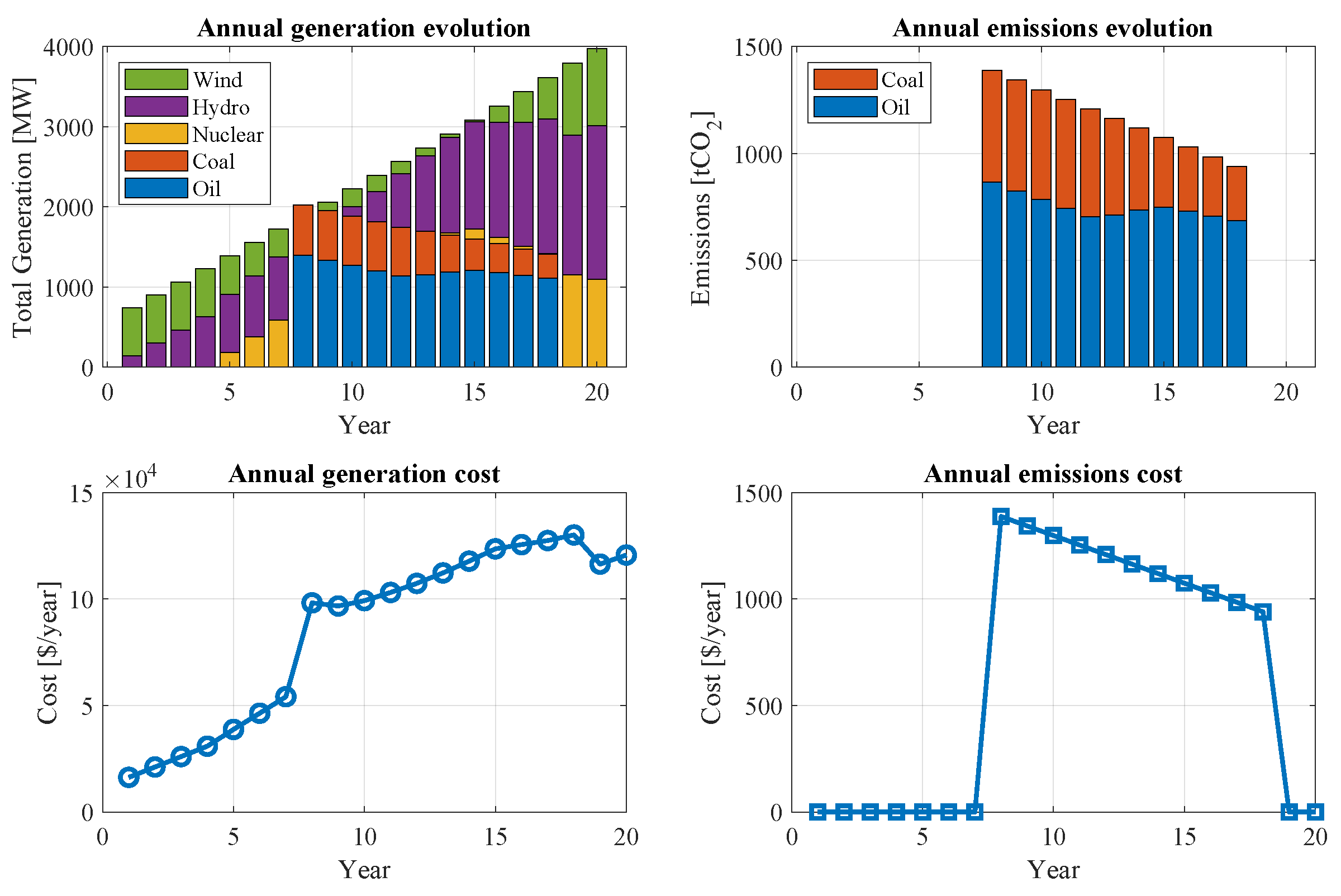
Figure 12.
Generation and demand behavior — gradual transition
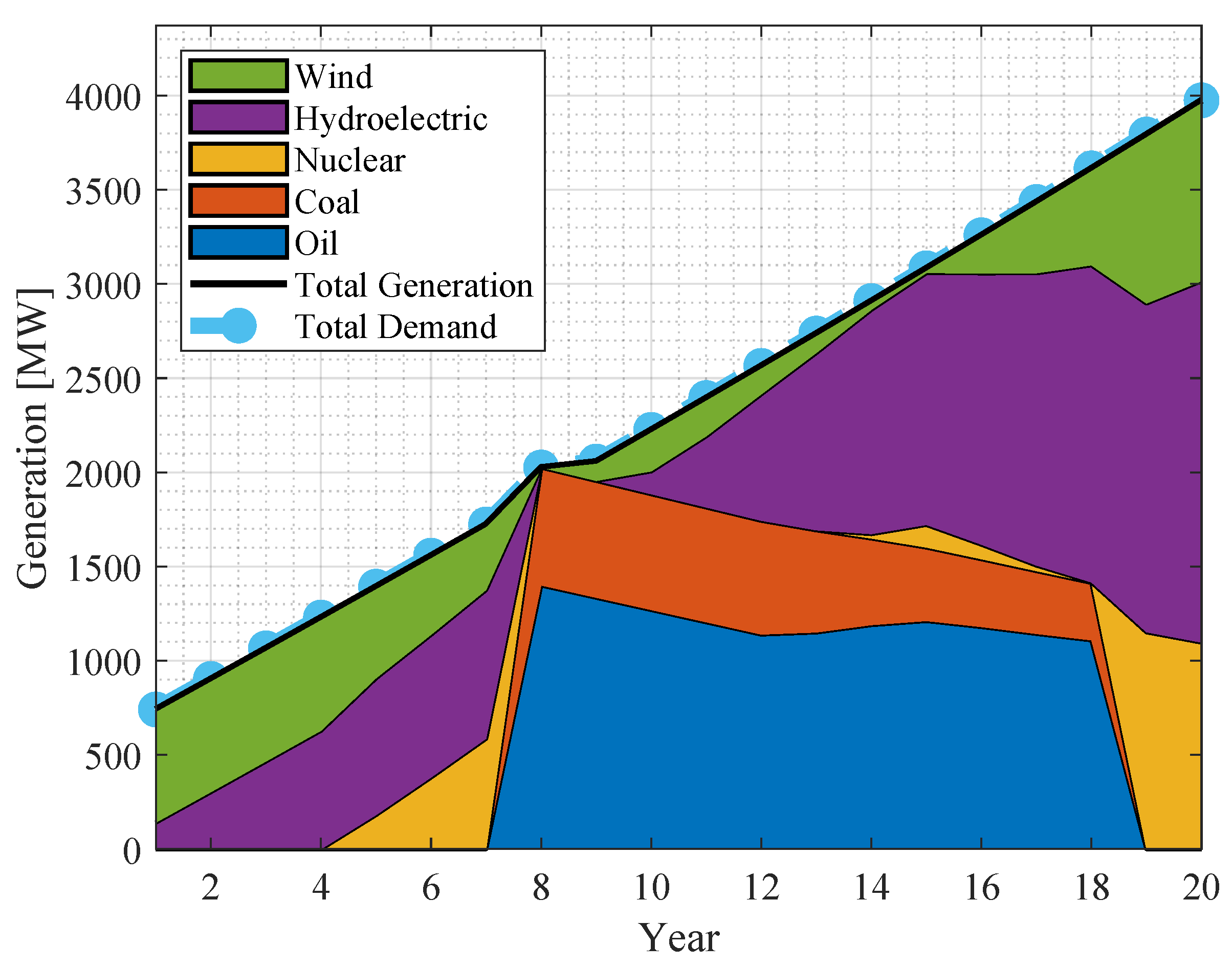
Figure 13.
Total power by technology — gradual transition
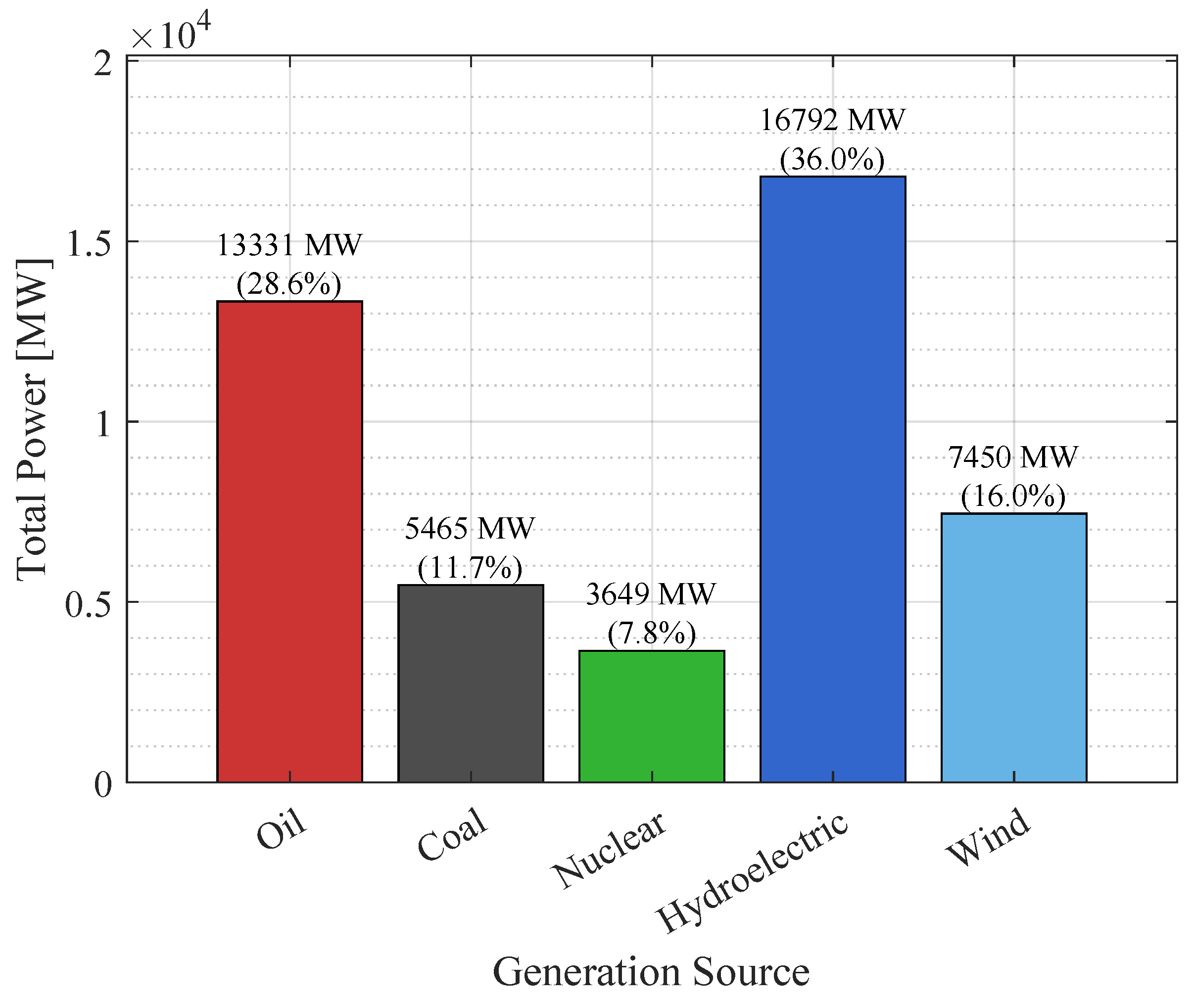
Figure 14.
Total emissions by technology — gradual transition
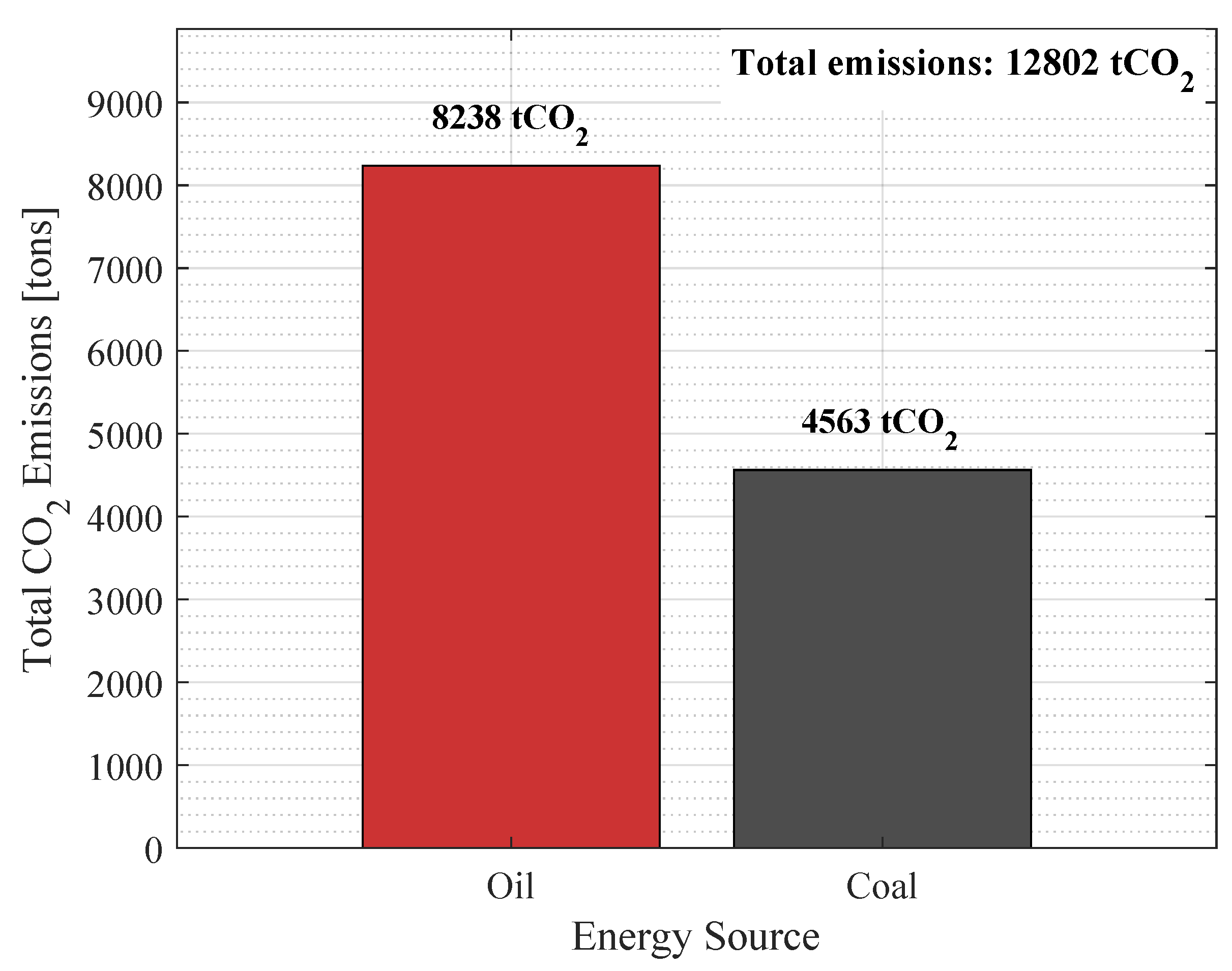
Figure 15.
Energy, environmental, and economic performance of the system during the planning horizon — accelerated transition
Figure 15.
Energy, environmental, and economic performance of the system during the planning horizon — accelerated transition
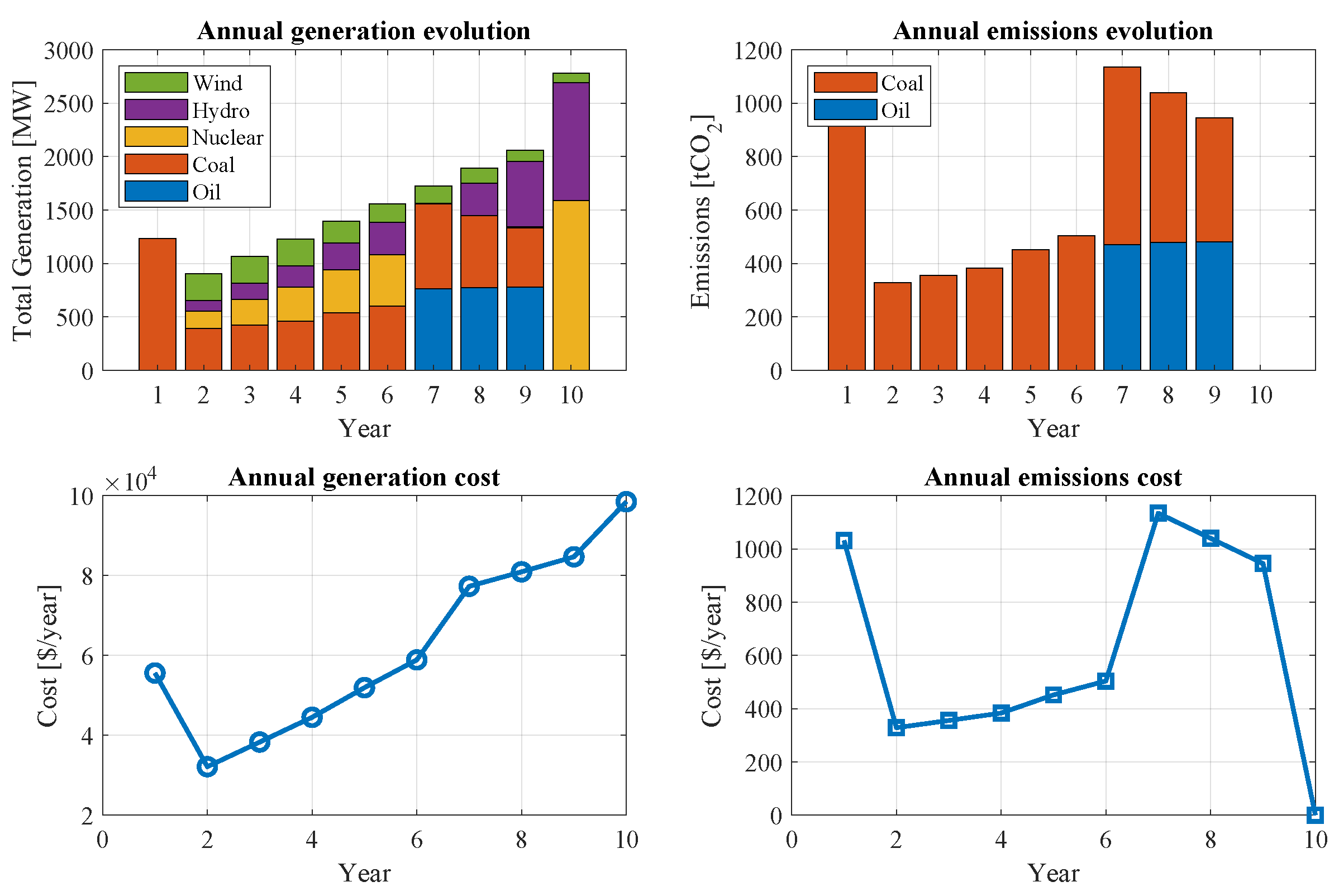
Figure 16.
Generation and demand behavior — accelerated transition
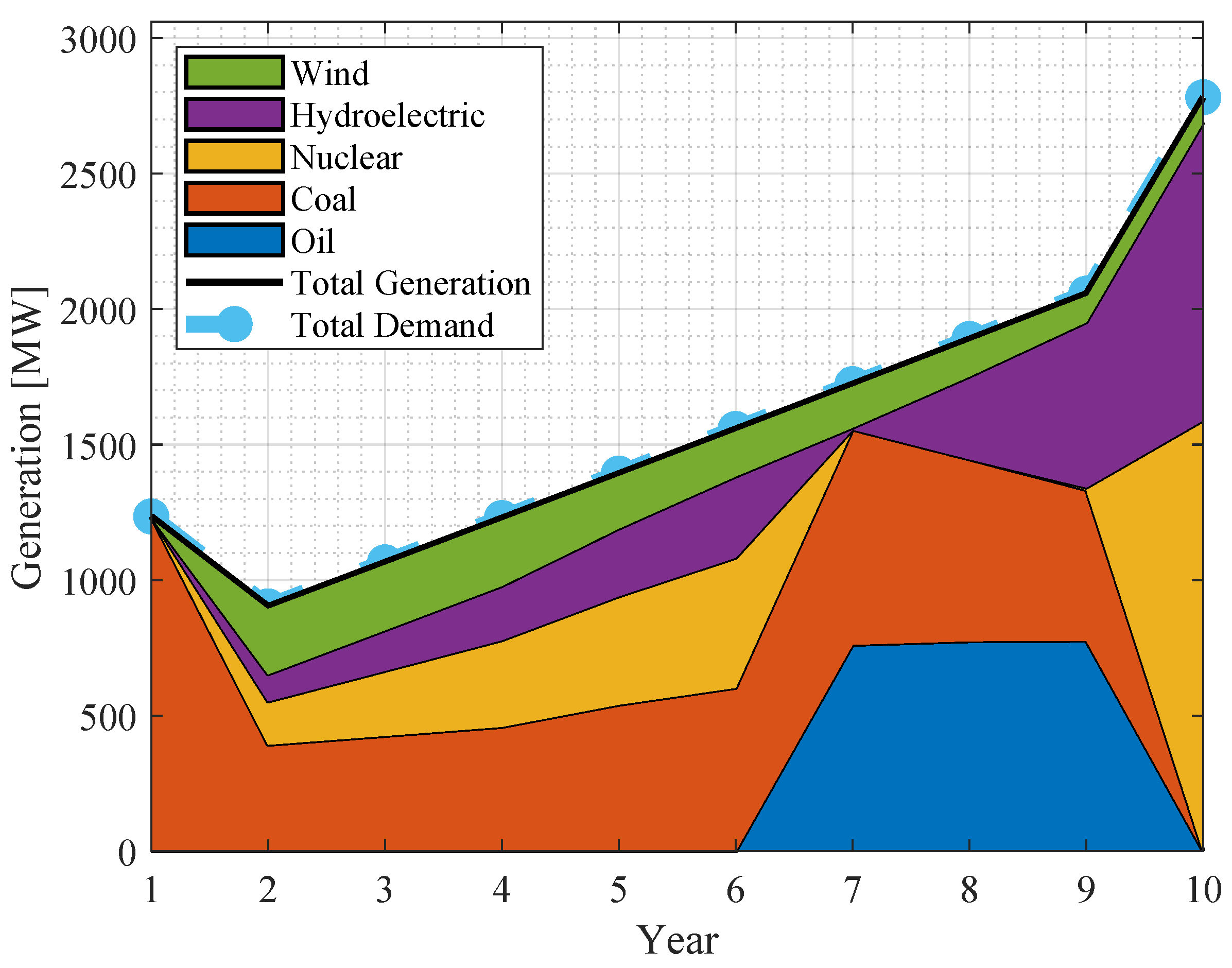
Figure 17.
Total power by technology — accelerated transition
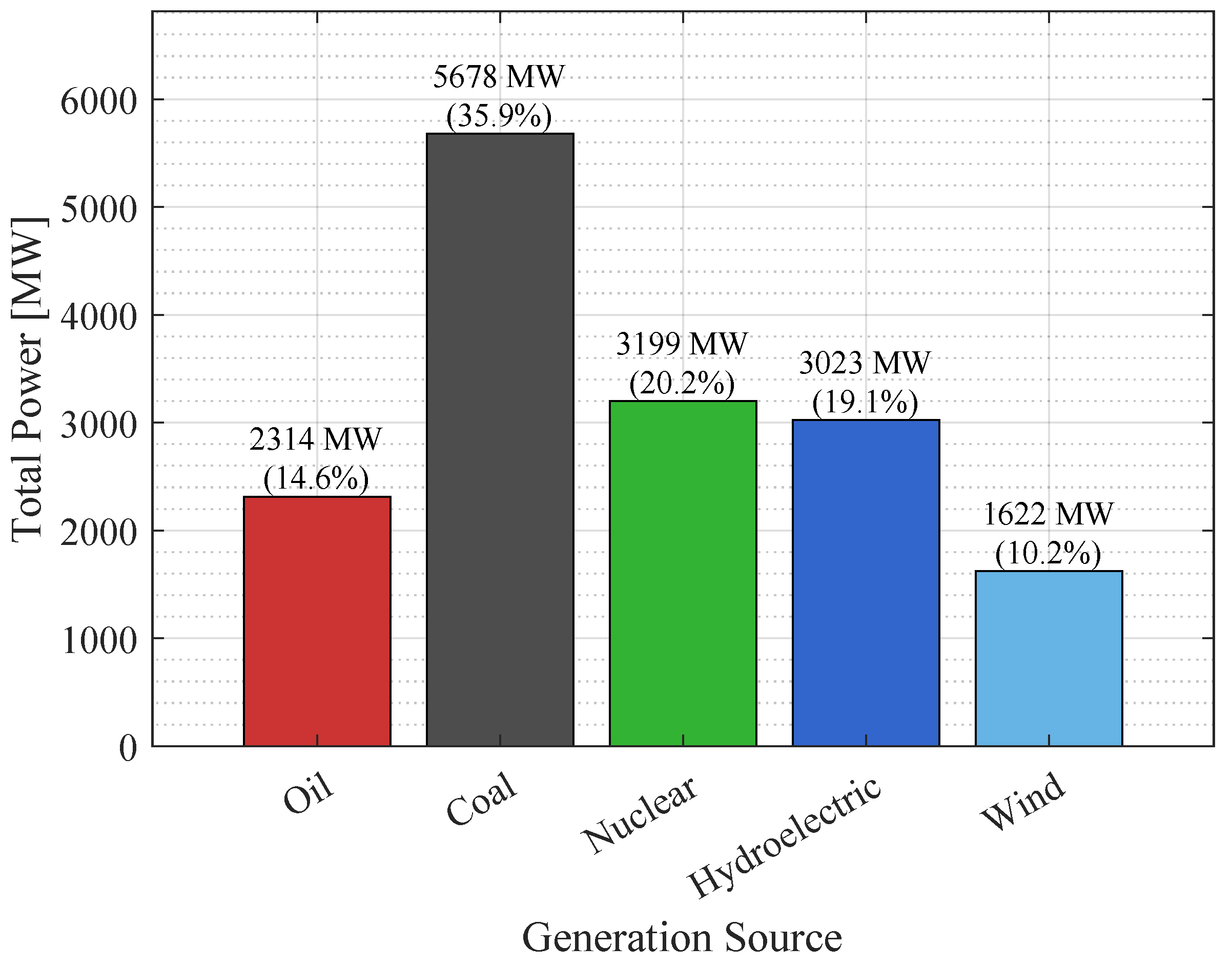
Figure 18.
Total emissions by technology — accelerated transition
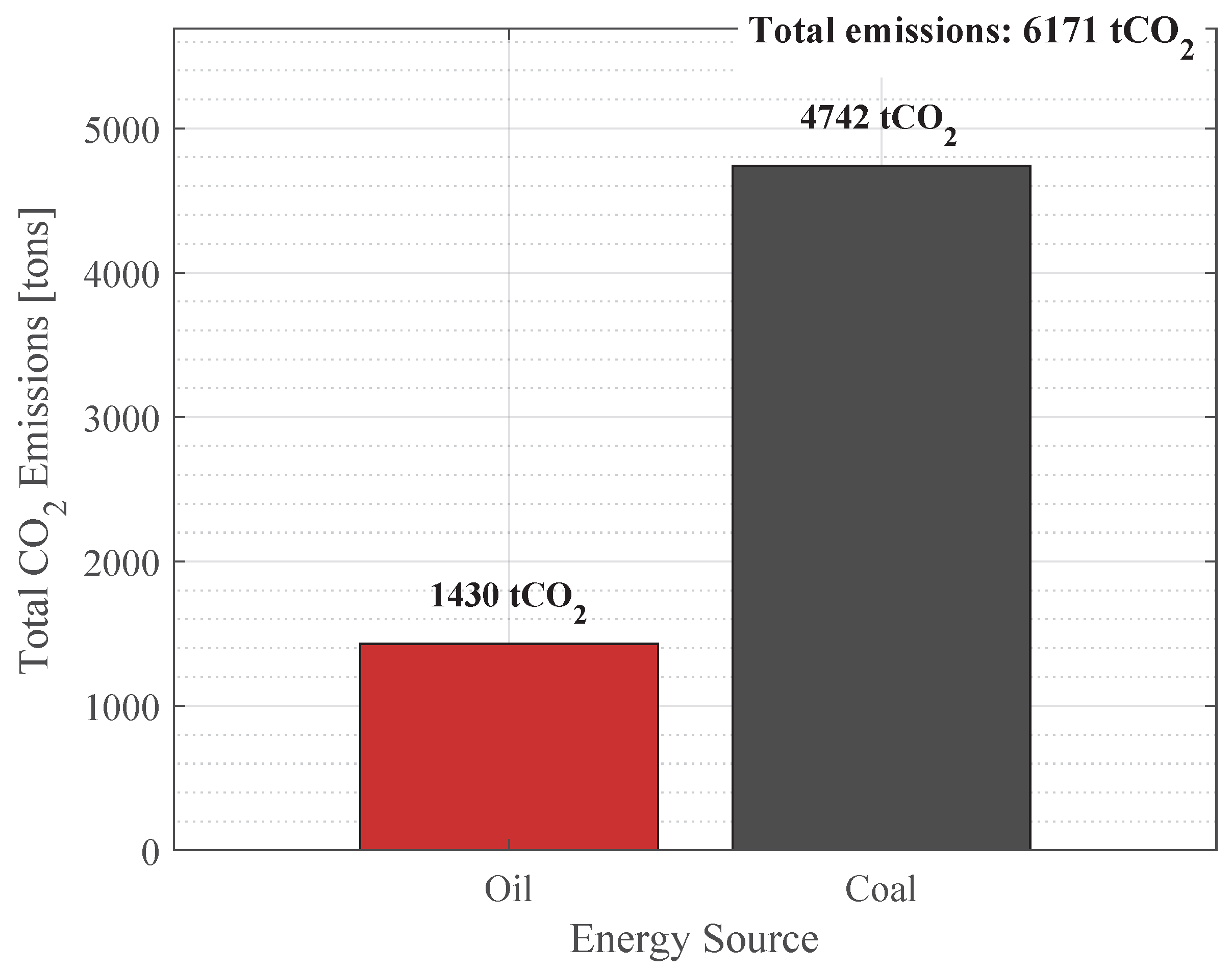
Table 1.
Effective and nominal capacity of power plants in Ecuador
| Plants | Energy Sources | Nominal Capacity [MW] |
Effective Capacity [MW] |
|---|---|---|---|
| Hydropower | Renewable | 5,106.85 | 5,072.26 |
| Photovoltaic | Renewable | 27.70 | 26.80 |
| Wind | Renewable | 21.20 | 21.20 |
| Biogas | Renewable | 8.40 | 7.25 |
| Biomass | Renewable | 144.40 | 136.45 |
| Thermal | Non-renewable | 3,426.15 | 2,836.90 |
Table 2.
Description of an ICE plant
| GUANGOPOLO II THERMAL POWER PLANT | |
|---|---|
| SUPERVISOR: | CELEC-EP/TERMOPICHINCHA |
| TECHNOLOGY TYPE: | Thermal Plant |
| GENERAL DATA | |
| Country | Ecuador |
| Province | Pichincha |
| City | Quito |
| Location | X X |
| TECHNICAL DATA | |
| Installed Capacity: | 52.38 MW |
| Type: | ICE |
| Number of Units: | 7 Units |
| Capacity per Unit: | 8.73 MW |
| Fuel Type: | Diesel–Bunker |
| Voltage: | - |
| Annual Energy: | 582.58 GWh |
| Plant Factor: | 3.82% |
| Engine: | |
| Type: | MITSUBISHI-MAN |
| Performance: | - |
| Rating: | 18 |
| RPM: | 5,200 kW |
| Quantity: | 400 |
| Frequency: | 60 Hz |
| Number of Phases: | 3 |
| Number of Poles: | - |
| Power Factor: | 0.80 |
| Engine: | |
| Type: | WÄRTSILÄ DIESEL |
| Performance: | 8SW28 |
| Rating: | 17 |
| RPM: | 1,980 kW |
| Quantity: | 900 |
| Frequency: | 60 Hz |
Table 3.
Description of a gas turbine plant.
| MACHALA II THERMAL POWER PLANT | |
|---|---|
| SUPERVISOR: | CELEC-EP/TERMOMACHALA |
| TECHNOLOGY TYPE: | Gas Turbine |
| GENERAL DATA | |
| Country | Ecuador |
| Province | El Oro |
| City | Machala |
| Location | X X |
| TECHNICAL DATA | |
| Installed Capacity: | 252 MW |
| Type: | Gas Turbine (GT) |
| Number of Units: | 8 Units |
| Capacity per Unit: | 6 of 20 MW and 2 of 66 MW |
| Fuel Type: | Natural Gas |
| Voltage: | - |
| Plant Factor: | 37.50% |
| Average Energy: | 406.70 |
| Gas Turbine | |
| Type: | General Electric |
| Model: | TM2500 |
| Rating: | - |
| RPM: | 1,980 kW |
| Quantity: | 900 |
| Frequency: | 60 Hz |
Table 4.
Description of a steam turbine plant.
| TRINITARIA THERMAL POWER PLANT | |
|---|---|
| SUPERVISOR: | CELEC-EP/ELECTROGUAYAS |
| TECHNOLOGY TYPE: | Steam Turbine Thermal Plant |
| GENERAL DATA | |
| Country | Ecuador |
| Province | Guayas |
| City | Guayaquil |
| Location | X X |
| TECHNICAL DATA | |
| Installed Capacity: | 133 MW |
| Type: | Steam Turbine (ST) |
| Number of Units: | 1 Unit |
| Capacity per Unit: | 133 MW |
| Fuel Type: | Fuel Oil #4 |
| Efficiency: | 16% |
| Voltage: | - |
| Plant Factor: | 54.10% |
| Average Energy: | 629.50 |
| Turbine | |
| Type: | DKY2-INDRI |
| Manufacturer: | ASEA BROWN BOVERI |
| Rating: | 133 kW |
| Quantity: | 1 |
| Rated Current: | 6.60 A |
| Frequency: | 60 Hz |
| Temperature: | 583 °C |
| Pressure: | 140 |
| Phases: | 3 |
| Poles: | 2 |
| Speed (RPM): | 3,600 |
Table 5.
Main actors in the Demand Response market.
| Actors | Offers | Users |
|---|---|---|
| BRP | Energy loss payments; Market access; DR incentives | Consumer |
| Aggregator | Ancillary services; Tariffs; Grid balancing services | TSO; DSO |
| Supplier/Retailer | Incentive packages and contracts for implicit DR programs; DR incentives | Consumers |
| Regulator | DR regulations; Knowledge for DR management | All actors |
| Consumer | Demand profile; Direct control; Large consumers can provide flexibility directly | Aggregator; Supplier/Retailer; DR market |
Table 6.
Pseudocode of the optimization model.
| Power System Decarbonization Process | |
| Step 1 |
Initialization Define main parameters: - Population size N - Maximum number of iterations or convergence criterion - Coefficient of variation of EECC < 5% - Parameters of genetic operators Initialize random solution population: Define binary variables: (installation of wind farm at node ) (ON/OFF status of generator at t) (activation of DR at node ) |
| Step 2 |
Evaluation of each solution in the population For each individual x in the population: Wind simulation and wind power generation: Use ARMA model for Calculate wind power output: Load modeling and demand response: Modify load curve: |
| Step 3 |
Calculation of optimization objectives Cost of Unserved Energy (EECC): Generation Cost (EGSC): Demand Response Cost (ELRC): Carbon Emissions (ECEC): |
| Continued on next page | |
| Continuation of Table 6 | |
| Step 4 |
Verification of constraints Generation-demand balance: Technical loss limit: Generation limits: Load shedding: Generator activation: Demand Response activation: |
| Step 5 |
Solution selection Identify non-dominated solutions in the population |
| Step 6 |
Fuzzy selection of the best solution For each individual x in the solution pool: For each objective : Normalize objective values Select the solution with the smallest error as optimal |
| Step 7 |
Genetic Operators Apply selection, crossover, and mutation on the solution set |
| Step 8 |
Convergence criterion If verification coefficient < 5% or iterations ≥ 100,000: Terminate algorithm Else: Update population and repeat from Step 2 |
| Step 9 |
Final result Return the solution set and the best solution |
| Step 10 | End |
| End of table | |
Table 7.
Variables used in Algorithm 1
| Symbol | Description | Unit |
|---|---|---|
| N | Population size | - |
| Wind penetration coefficients for each generator | - | |
| Percentage of load to be shifted in each load sector | - | |
| Wind speed | m/s | |
| Cut-in, rated, and cut-out wind speeds of the turbine | m/s | |
| Rated power of the wind turbine | MW | |
| Coefficients of the wind power function | - | |
| Load demand at time t | MW | |
| Power shifted by demand response | MW | |
| Set of simulation periods | - | |
| Power generated by the wind farm | MW | |
| Unserved energy losses | MW | |
| Value of Lost Load | $/MW | |
| Energy reduced by demand response | MWh | |
| Incentive cost for load reduction | $ | |
| Oil-fired generation cost | $/MWh | |
| Fixed cost of oil-fired generation | $ | |
| Energy generated with oil | MWh | |
| Oil generation emission factors | ton CO2/MWh | |
| Power generated by unit g | MW | |
| Power demanded in sector l | MW | |
| Minimum and maximum generation limits | MW |
Table 8.
Generation system data
| Fuel | Technology | Node | Capacity [MW] |
|---|---|---|---|
| Oil | Combustion turbine | 1 | 40 |
| 2 | 40 | ||
| Steam turbine | 7 | 300 | |
| 13 | 591 | ||
| 15 | 60 | ||
| Coal | Steam turbine | 15 | 155 |
| 16 | 155 | ||
| 23 | 660 | ||
| Water | Nuclear steam | 18 | 400 |
| 21 | 400 | ||
| Water | Hydraulic turbine | 22 | 300 |
Table 11.
Carbon emission rates and costs by technology
| Fuel | Technology | CE [tonCO2/MWh] |
EC [$/tonCO2] |
|---|---|---|---|
| Oil | Combustion turbine | 0.618 | 35 |
| Steam turbine | - | - | |
| Coal | Steam turbine | 0.743 | 35 |
| Water | Nuclear steam | 0.835 | - |
| Water | Hydraulic turbine | - | - |
| Wind | Wind turbine | - | - |
Table 12.
Load interruption cost by customer segment due to rescheduling
| Load type | IC [$/MWh] |
|---|---|
| Residential | 150 |
| Industrial | 13930 |
| Commercial | 12870 |
| Large consumers | 13930 |
| Agriculture | 650 |
| Government | 3460 |
| Office | 3460 |
Disclaimer/Publisher’s Note: The statements, opinions and data contained in all publications are solely those of the individual author(s) and contributor(s) and not of MDPI and/or the editor(s). MDPI and/or the editor(s) disclaim responsibility for any injury to people or property resulting from any ideas, methods, instructions or products referred to in the content. |
© 1996 by the authors. Licensee MDPI, Basel, Switzerland. This article is an open access article distributed under the terms and conditions of the Creative Commons Attribution (CC BY) license (https://creativecommons.org/licenses/by/4.0/).
Copyright: This open access article is published under a Creative Commons CC BY 4.0 license, which permit the free download, distribution, and reuse, provided that the author and preprint are cited in any reuse.


